FedPD: A Federated Learning Framework with Optimal Rates and Adaptivity to Non-IID Data
Abstract
Federated Learning (FL) is popular for communication-efficient learning from distributed data. To utilize data at different clients without moving them to the cloud, algorithms such as the Federated Averaging (FedAvg) have adopted a “computation then aggregation” (CTA) model, in which multiple local updates are performed using local data, before sending the local models to the cloud for aggregation. These algorithms fail to work when facing practical challenges, e.g., the local data being non-identically independent distributed. In this paper, we first characterize the behavior of the FedAvg algorithm, and show that without strong and unrealistic assumptions on the problem structure, it can behave erratically (e.g., diverge to infinity). Aiming at designing FL algorithms that are provably fast and require as few assumptions as possible, we propose a new algorithm design strategy from the primal-dual optimization perspective. Our strategy yields algorithms that can deal with non-convex objective functions, achieve the best possible optimization and communication complexity (in certain sense), and deal with full-batch and mini-batch local computation models. Importantly, the proposed algorithms are communication efficient, in that the communication effort can be reduced when the level of heterogeneity among the local data also reduces. To our knowledge, this is the first algorithmic framework for FL that achieves all the above properties.
1 Introduction
Federated learning (FL)—a distributed machine learning approach proposed in [1]—has gained popularity for applications involving learning from distributed data. In FL, a cloud server (the “server”) can communicate with distributed data sources (the “agents”). The goal is to train a global model that works well for all the distributed data, but without requiring the agents to reveal too much local information. Since its inception, the broad consensus on FL’s implementation appears to involve a generic “computation then aggregation” (CTA) protocol. This involves the following steps: S1) the server sends the model to the agents; S2) the agents update their local models ’s for several iterations based on their local data; S3) the server aggregates ’s to obtain a new global model . It is widely acknowledged that multiple local steps save communication efforts, while only transmitting local models protects data privacy [2].
Even though the FL paradigm has attracted significant research from both academia and industry, and many algorithms such as Federated Averaging (FedAvg) have been proposed, several attributes are not clearly established. In particular, the commonly adopted CTA protocol poses significant theoretical and practical challenges to designing effective FL algorithms. This work attempts to provide a deeper understanding of FL, by raising and resolving a few theoretical questions, as well as by developing an effective algorithmic framework with several desirable features.
Problem Formulation. Consider the vanilla FL solving the following problem:
| (1) |
where is the number of agents; denotes one sample in data set stored on the -th agent; is the “loss function” for the -th data point; and is a “weight coefficient” (a common choice is [2]). We assume that the loss function takes the same form across different agents, and furthermore, we denote to be the total number of samples. One can also consider a related setting, where each represents the expected loss [3]
| (2) |
where denotes the data distribution on the -th agent. Throughout the paper, we will make the following blanket assumptions for problem (1):
A 1.
Each , as well as in (1) is –smooth:
A 2.
The objective of problem (1) is lower bounded: , .
In addition to these standard assumptions, state-of-the-art efforts on analysis of FL algorithms oftentimes invoke a number of more restrictive assumptions.
A 3.
(Bounded Gradient (BG)) The gradients ’s are upper bounded (by a constant )
| (3) |
A 4.
(I.I.D. Data) Either one of the following holds:
| (4) | ||||
| (5) |
Let us comment on the above assumptions.
First, the BG assumption typically does not hold for (1), in particular, (where and are related to data). However, the BG assumption is critical for analyzing FedAvg-type algorithms because it bounds the distance traveled after multiple local iterates. Second, (4) is typically used in FL to characterize homogeneity about local data [4, 5]. However, an assumption of this type does not hold for FL applications where the data (such as medical records, keyboard input data) are generated by the individual agents [1, 3, 6, 7, 8, 9]. A reasonable relaxation to this i.i.d. assumption is the following notion of -non-i.i.d.-ness of the data distribution.
A 5.
(-Non-I.I.D. Data) The local functions are called -non-i.i.d. if either one of the equivalent conditions below holds:
| (6) |
By varying from to , (6) provides a characterization of data non-i.i.d.-ness. In Appendix A, we give a few examples of loss functions with different values of . Note that the second inequality in (6) is often used in decentralized optimization to quantify the similarity of local problems [10, 11]. Third, (5) does not hold for many practical problems. To see this, note that this condition is parameterized by , which is typically the desired optimization accuracy [12]. Since can be chosen arbitrarily small, (5) essentially requires that the problem is realizable, that is, approaches zero only when all the local gradients approach zero at , that is, when the local data are “similar”.
Finally, we mention that our objective is to understand FL algorithm from an optimization perspective. So we say that a solution is an -stationary solution if the following holds:
| (7) |
We are interested in finding the minimum system resources required, such as the number of local updates, the number of times local variables are transmitted to the server, and the number of times local samples ’s are accessed, before computing an -solution (7). These quantities are referred to as local computation, communication complexity, and sample complexities, respectively.
Questions to address Despite extensive recent research, the FL framework, and in particular, the CTA protocol is not yet well understood. Below, we list four questions regarding the CTA protocol.
Q1 (local updates). What are the best local update directions for the agents to take so as to achieve the best overall system performance (stability, sample complexity, etc.)?
Q2 (global aggregation). Can we use more sophisticated processing in the aggregation step to help improve the system performance (sample or communication complexity)?
Q3 (communication efficiency). If multiple local updates are preformed between two aggregation steps, will it reduce the communication overhead?
Q4 (assumptions). What is the best performance that the CTA type algorithms can achieve while relying on a minimum set of assumptions about the problem?
Although these questions are not directly related to data privacy, another important aspect of FL, we argue that answering these fundamental questions can provide much needed understanding on algorithms following the CTA, and thus the FL approach. A few recent works (to be reviewed shortly) have touched upon those questions, but to our knowledge, none of them has conducted a thorough investigation of the questions listed above.
Related Works. We start with a popular method following the CTA protocol, the FedAvg in Algorithm 1, which covers the original FedAvg [1], the Local SGD [4], PR-SGD [13, 3] and the RI-SGD [14] among others.
In FedAvg, is the total stage number, the number of local updates, the index of the stage, the index of the inner iteration, and ’s are the stepsizes. It has two options for local updates:
| (8) | |||
| (9) |
Many recent works are extensions of FedAvg. The algorithm proposed in [3] adds momentum to the algorithm. In [14], the data on the local agents are separated into blocks and shared with other agents. In [15] the local GD version (9) is studied. In [5], a cooperative-SGD is considered; it includes virtual agents, extra variables, and relaxes the parameter server topology.
It is pertinent to consider how these algorithms address questions Q1–Q4. For Q1, most FedAvg-type algorithms perform multiple local (stochastic) GD steps to minimize the local loss function. However, we will see shortly that in many cases, successive local GD steps lead to algorithm divergence. For Q2, most algorithms use simple averaging, and there is little discussion on whether other types of (linear) processing will be helpful. For Q3, a number of recent works such as [3, 15] show that, for non-convex problems, to achieve -solution (7), a total of aggregation steps are needed. However, it is not clear if this achieves the best communication complexity. As for Q4, the FedAvg-type algorithm typically requires either some variant of the BG assumption, or some i.i.d. assumption, or both; See Table 1 rows 1–5 for detailed discussions.
A number of more recent works have improved upon FedAvg in various aspects. FedProx [12] addresses Q1 and Q4 by perturbing the update direction. This algorithm does not need the BG, but it still requires the i.i.d. assumption (5). The VRL-SGD proposed in [16] addresses Q1 and Q4 by using the variance reduction (VR) technique to update the directions for local agents and achieves communication complexity without the i.i.d. assumption. F-SVRG [17] is another recent algorithm that uses VR. This algorithm does not follow the CTA protocol as the agents have to transmit the local gradients, but it does not require A3 and A4. The PR-SPIDER [18] further improves upon FSVRG by reducing sample complexity (SC) from to (where is typically larger than ). Although FSVRG and PR-SPIDER neither require the BG or the i.i.d. assumptions, they require the agents to transmit local gradients to the server and thus do not follow the CTA protocol. This is undesirable, as it has been shown that local gradient information can leak private data [19]. Additionally, questions Q2-Q3 are not addressed in these works.
| Algorithm | Convexity | DN | BG | RC () | LC () | AS |
| FedAvg [4] | SC | 0 | No | |||
| FedAvg [9] | SC | - | Yes | |||
| Coop-SGD [5] | NC | 0 | No | |||
| MPR-SGD [3] | NC | - | Yes | |||
| Local-GD [15] | C | - | No | |||
| FedProx [12] | NC | - | No | |||
| F-SVRG[17] | NC | - | No | |||
| VRL-SGD[16] | NC | - | Yes⋆ | |||
| Fed-PD-GD | NC | No | ||||
| Fed-PD-SGD | NC | No | ||||
| Fed-PD-VR | NC | - | No |
Our Main Contributions. First, we address Q1-Q4 and provide an in-depth examination of the CTA protocol. We show that algorithms following the CTA protocol that are based on successive local gradient updates, the best possible communication efficiency is ; neither additional local processing nor general linear processing can improve this rate. We then show that the BG and/or i.i.d. data assumption is important for the popular FedAvg to work as intended.
Our investigation suggests that the existing FedAvg-based algorithms are (provably) insufficient in dealing with many practical problems, calling for a new design strategy. We then propose a meta-algorithm called Federated Primal-Dual (FedPD), which also follows the CTA protocol and can be implemented in several different forms with desirable properties. In particular, it i) can deal with the general non-convex problem, ii) achieve the best possible optimization and communication complexity when data is non-i.i.d., iii) achieve convergence under only Assumptions A1– A2.
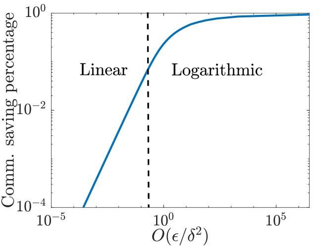
Most importantly, the communication pattern of the proposed algorithm can be adapted to the degree of non-i.i.d.-ness of the local data. That is, we show that under the -non-i.i.d. condition (6), communication saving and data heterogeneity interestingly exhibit a linear-logarithmic relationship; see Fig. 1 for an illustration. To our knowledge, this is the first algorithm for FL that achieves all the above properties.
2 Addressing Open Questions
We first address Q2–Q3. Specifically, for problems satisfying A1–A2, does performing multiple local updates or using different ways to combine local models reduce communication complexity? We show that such a saving is impossible; there exist problems satisfying A1–A2, yet no matter what types of linear combinations the server performs, as long as the agents use local gradients to update the model, it takes at least communication rounds to achieve an -stationary solution (7). Consider the following generic CTA protocol. Let denote the index for communication rounds. Between two rounds and , each agent performs local updates. Denote to be the -th local update. Then, ’s are sent to the server, combined through a (possibly time-varying) function , and sent back. The agents then generate a new iterate, by combining the received message with past gradients using a (possibly time-varying) function :
| (10a) | ||||
| (10b) | ||||
We focus on the case where the ’s and ’s are linear operators, which implies that can use all past iterates and (sample) gradients for its update. Clearly, (10) covers both the local-GD and local-SGD versions of FedAvg as special cases. In the following, we provide an informal statement of the result. The formal statement and the full proof are given in Appendix B and Theorem 2.
Claim 2.1.
(Informal) Consider any algorithm that belongs to the class described in (10), with and ’s being linear and possibly time-varying operators. Then, there exists a non-convex problem instance satisfying Assumptions 1–2 such that for any , algorithm takes at least communication rounds to reach an -stationary solution satisfying (7).
Remark 1. The proof technique is related to those developed from both classical and recent works that characterize lower bounds for first-order methods, in both centralized [20, 21] and decentralized [22, 23] settings. The main technical difference is that our processing model (10) additionally allows local processing iterations, and there is a central aggregator. Our goal is not to establish lower bounds on the number of (centralized) gradient access, nor to show the optimal graph dependency, but to characterize (potential) communication savings when allowing multiple steps of local processing.
In the proof, we construct difficult problem instances in which ’s are not i.i.d. (more precisely, in assumption (4) grows with the total number of iterations ). Then we show that it is necessary to aggregate (thus communicate) to make any progress. On the other hand, it is obvious that in another extreme case where the data are -non-i.i.d., only communication rounds are needed. An open question is: when the local data are related to each other, i.e., lies between and infinity, is it possible to reduce the total communication rounds? This question is addressed below in Sec. 3.
We now address Q1 and Q4. We consider the FedAvg Algorithm 1, and show that BN and/or i.i.d. assumptions are critical for them to perform well. Our result suggests that, despite its popularity, components in FedAvg, such as the pure local (stochastic) gradient directions and linear aggregation are not compatible with each other. The proof of the results below are given in Appendix C.
Claim 2.2.
Remark 2. A recent work [15] has shown that FedAvg with constant stepsize can only converge to a neighborhood of the global minimizer for convex problems. Moreover, the error to the global optima is related to and the degree of non-i.i.d.-ness as measured by the size of where is the global optimal solution. On the other hand, our result indicates that when ’s are non-convex, FedAvg can perform much worse without the BN and the i.i.d. assumption. Even if and there exists a solution such that , FedAvg (with constant stepsize ) diverges and the iteration can go to .
One may think that using a constant stepsize is the culprit for the divergence in Claim 2.2. In fact, we can show that having BG or not can still impact the performance of FedAvg, even when diminishing stepsize is used. In particular, we show in Appendix D, that FedAvg converges under the BG assumption for any diminishing stepsize, but without it, the choice of the stepsize can be significantly restricted.
3 The FedPD Framework
The previous section reveals a number of properties about FedAvg and, broadly speaking, the CTA protocol. But why does FedAvg only work under very restrictive conditions? Is it because the local update directions are not chosen correctly? Is it possible to make it work without any additional assumptions? Can we reduce communication effort when the local data becomes more i.i.d.?
In this section, we propose a meta-algorithm called Federated Primal-Dual (FedPD), which can be specialized into different sub-variants to address the above questions. These algorithms possess a few desirable features: They can achieve the best optimization and communication complexity when data is non-i.i.d. (i.e., achieving the bounds in Claim 2.1); they only require A1 –A2, while being able to utilize both full or sampled local gradients. Most importantly, the communication pattern of the proposed algorithm can be made adaptive to the degree of data non-i.i.d.-ness across the agents.
3.1 The Proposed Algorithm
Our algorithm is based on the following global consensus reformulation of the original problem (1):
| (11) |
Similar to traditional primal-dual based algorithms [24], the idea is that, when relaxing the equality constraints, the resulting problem is separable across different nodes. However, different from ADMM, the agents can now perform either a single (or multiple) local update(s) between two communication rounds. Importantly, such flexibility makes it possible to adapt the communication frequency to the degree of -non-i.i.d.-ness of the local data. In particular, we identify that under -non-i.i.d. (4), the fraction is the key quantity that determines communication saving; see Fig. 1. Intuitively, significant reduction can be achieved when is smaller than ; otherwise, the reduction goes to zero linearly as increases. To our knowledge, none of the existing ADMM based algorithms, nor FL based algorithms, are able to provably achieve such a reduction.
To present our algorithm, let us define the augmented Lagrangian (AL) function of (11) as
Fixing , the AL is separable over all local pairs . The key technique in the design is to specify how each local AL should be optimized, and when to perform model aggregation.
Federated primal-dual algorithm (FedPD) captures the main idea of the classical primal-dual based algorithm while meeting the flexibility need of FL; see Algorithm 2. In particular, its update rules share a similar pattern as ADMM, but it does not specify how the local models are updated. Instead, an oracle is used as a placeholder for local processing, and we will see that careful instantiations of these oracles lead to algorithms with different properties. Importantly, we introduce a critical constant , which determines the frequency at which the aggregation and communication steps are skipped. In Algorithm 3 and Algorithm 4, we provide two useful examples of the local oracles.
In Algorithm 3, ’s are chosen so that the local problems are solved accurately enough to satisfy:
| (12) |
We provide two ways for solving this subproblem by using GD and SGD, but any other solver that achieves (12) can be used. For the SGD version, the stochastic gradient is defined as
| (13) |
where denotes uniform sampling. Despite the simplicity of the local updates, we will show that using Oracle I makes FedPD adaptive to the non-i.i.d. parameter .
3.2 Convergence and Complexity Analysis
We analyze the convergence of FedPD with Oracle I. The detailed proofs are given in Appendix F. The convergence analysis of FedPD with an alternative Oracle is given in Appendix G
Theorem 1.
Case I) Suppose A5 holds with . Set , . Then we have:
Case II) Suppose , , and A5 holds with a finite . Then we have:
| (14) |
Here are constants independent of ; .
Remark 3. (Communication complexity) Case I says if one does not skip communication (), then to achieve -stationarity (i.e., for some ), they need to set , , and the total communication rounds is .
In Case II, the second term on the right hand side of (14) involves both and , so we can select them appropriately to reduce communication while maintaining the same accuracy. Specifically, we choose and . Then we have
Then we can achieve the same -accuracy as Case I. The communication rounds here is .
The relation between the saving and is showed in Table 2. Roughly speaking, is inversely proportional to degree of non-i.i.d-ness when ; further, at a log-rate when . Our result also indicates that, when using stage-wise training for neural networks, the algorithm can communicate less at the early stages since they typically have lower accuracy target to enable larger stepsizes [25].
| Range of | as function of | Relation | ||
|---|---|---|---|---|
| Linear | ||||
| Log |
Remark 4. (Computation complexity) To achieve accuracy, we need both and . As the local AL is strongly convex with respect to , optimizing it to accuracy requires iterations for GD and for SGD [26]. So the total number of times that the local gradients (respectively, stochastic gradients) are accessed is given by (respectively, ).
3.3 Connection with Other Algorithms
Before we close this section, we discuss the relation of FedPD with a few existing algorithms.
The FedProx/FedDANE In FedProx [12] the agents optimize the following local objective: . This fails to converge to the global stationary solution. In contrast, FedPD introduces extra local dual variables that record the gap between the local model and the global model which help the global convergence. FedDANE [27] also proposes a way of designing the subproblem by using the global gradient, but this violates the CTA protocol. Compared with these two algorithms, the proposed FedPD has weaker assumptions, and it achieves better sample and/or communication complexity.
Event Triggering Algorithms. A number of recent works such as Lazily Aggregated Gradient (LAG) [28] and COLA [29] have been proposed to occasionally skip message exchanges among the agents to save communication. In LAG, each agent receives the global model every iteration, and decides whether to send some local gradient differences by checking certain conditions. Since gradient information is transmitted, LAG does not belong to the algorithm class (10). When the local problems are unbalanced, in the sense that the discrepancy between the local Lipschitz gradients ’s is large, then the agents with smaller ’s can benefit from the lazy aggregation. Meanwhile, instead of measuring whether the local problems are balanced, the -non-i.i.d. criteria characterizes if local problems are similar by measuring the uniform difference between arbitrary pairs of the local problems. If the data is i.i.d., then the agents benefit equally from the communication reduction.
4 Numerical Experiments
In the first experiment, we show the convergence of the proposed algorithms on synthetic data with FedAvg and FedProx as baselines. We use the non-convex penalized logistic regression [30] as the loss function. We use two ways to generate the dataset, in the first case (referred to as the “weakly non-i.i.d” case), the data is generated in an i.i.d. way. In the second case (referred to as the “strongly non-i.i.d” case), we generate the data using non-i.i.d. distribution. In both cases there are samples on each agent with total agents.
We run FedPD with Oracle I (FedPD-SGD and FedPD-GD) and Oracle II (FedPD-VR). For FedPD-SGD, we set , and for FedPD-GD and FedPD-VR we set . For FedPD-GD we set and , wherein the later case the agents skips half of the communication rounds. For FedPD-VR, we set mini-batch size and gradient computation frequency . For comparison, we also run FedAvg with local GD/SGD and FedProx. For FedAvg with GD, , and for FedAvg with SGD, . For FedProx, we solve the local problem using variance reduction for iterations. The total number of iterations is set as for all algorithms.
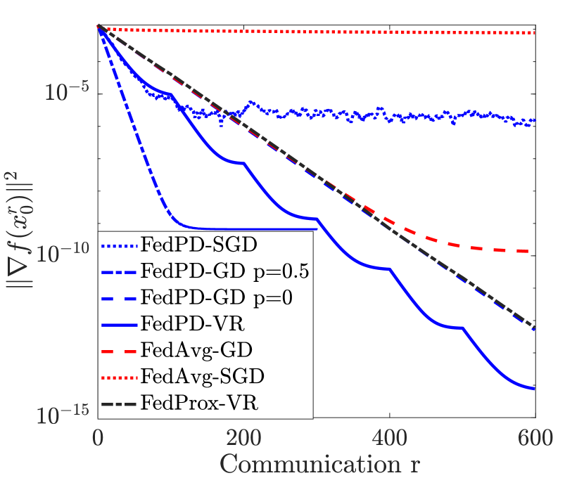
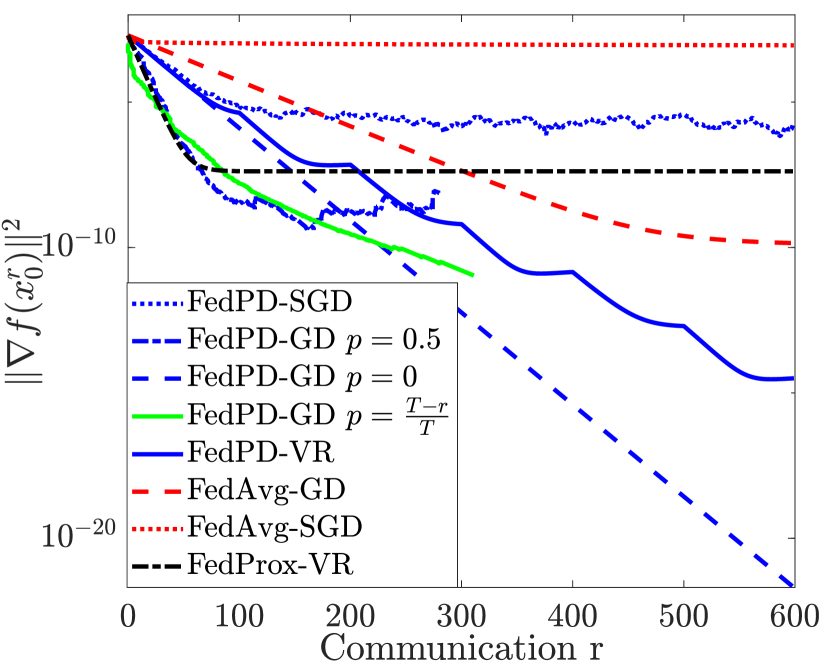
Fig. 2 shows the results with respect to the number of communication rounds. In Fig. 2(a), we compare the convergence of the tested algorithms on weakly non-i.i.d. data set. It is clear that FedProx and FedPD with (i.e., no communication skipping) are comparable. Meanwhile, FedAvg with local GD will not converge to the stationary point with a constant stepsize when local update step . By skipping half of the communication, FedPD with local GD can still achieve a similar error as FedAvg, but using fewer communication rounds. In Fig. 2(b), we compare the convergence results of different algorithms with the strongly non-i.i.d. data set. We can see that the algorithms using stochastic solvers become less stable compared with the case when the data sets are weakly non-i.i.d. Further, FedPD-VR and FedPD-GD with are able still to converge to the global stationary point while FedProx will achieve a similar error as the FedAvg with local GD.
We included more details on the experimental results and additional experiments in Appendix H.
5 Conclusion
We study federated learning under the CTA protocol. We explore a number of theoretical properties of this protocol, and design a meta-algorithm called FedPD, which contains various algorithms with desirable properties, such achieving the best communication/computation complexity, as being able to adapt its communication pattern with data heterogeneity.
References
- [1] Jakub Konečnỳ, H Brendan McMahan, Felix X Yu, Peter Richtárik, Ananda Theertha Suresh, and Dave Bacon, “Federated learning: Strategies for improving communication efficiency,” arXiv preprint arXiv:1610.05492, 2016.
- [2] Tian Li, Anit Kumar Sahu, Ameet Talwalkar, and Virginia Smith, “Federated learning: Challenges, methods, and future directions,” arXiv preprint arXiv:1908.07873, 2019.
- [3] Hao Yu, Rong Jin, and Sen Yang, “On the linear speedup analysis of communication efficient momentum SGD for distributed non-convex optimization,” in Proceedings of the 36th International Conference on Machine Learning, Kamalika Chaudhuri and Ruslan Salakhutdinov, Eds., Long Beach, California, USA, 09–15 Jun 2019, vol. 97 of Proceedings of Machine Learning Research, pp. 7184–7193, PMLR.
- [4] Sebastian Urban Stich, “Local sgd converges fast and communicates little,” ICLR 2019 - International Conference on Learning Representations, p. 17, 2019.
- [5] Jianyu Wang and Gauri Joshi, “Cooperative SGD: A unified framework for the design and analysis of communication-efficient sgd algorithms,” arXiv preprint arXiv:1808.07576, 2018.
- [6] X. Wang, Y. Han, C. Wang, Q. Zhao, X. Chen, and M. Chen, “In-edge AI: Intelligentizing mobile edge computing, caching and communication by federated learning,” IEEE Network, vol. 33, no. 5, pp. 156–165, Sep. 2019.
- [7] Virginia Smith, Chao-Kai Chiang, Maziar Sanjabi, and Ameet S Talwalkar, “Federated multi-task learning,” in Advances in Neural Information Processing Systems 30, I. Guyon, U. V. Luxburg, S. Bengio, H. Wallach, R. Fergus, S. Vishwanathan, and R. Garnett, Eds., pp. 4424–4434. Curran Associates, Inc., 2017.
- [8] Keith Bonawitz, Hubert Eichner, Wolfgang Grieskamp, Dzmitry Huba, Alex Ingerman, Vladimir Ivanov, Chloe Kiddon, Jakub Konecny, Stefano Mazzocchi, H Brendan McMahan, et al., “Towards federated learning at scale: System design,” arXiv preprint arXiv:1902.01046, 2019.
- [9] Xiang Li, Kaixuan Huang, Wenhao Yang, Shusen Wang, and Zhihua Zhang, “On the convergence of fedavg on non-iid data,” arXiv preprint arXiv:1907.02189, 2019.
- [10] Xiangru Lian, Ce Zhang, Huan Zhang, Cho-Jui Hsieh, Wei Zhang, and Ji Liu, “Can decentralized algorithms outperform centralized algorithms? a case study for decentralized parallel stochastic gradient descent,” in Advances in Neural Information Processing Systems, 2017.
- [11] Shiqiang Wang, Tiffany Tuor, Theodoros Salonidis, Kin K Leung, Christian Makaya, Ting He, and Kevin Chan, “When edge meets learning: Adaptive control for resource-constrained distributed machine learning,” in IEEE INFOCOM 2018-IEEE Conference on Computer Communications. IEEE, 2018, pp. 63–71.
- [12] Anit Kumar Sahu, Tian Li, Maziar Sanjabi, Manzil Zaheer, Ameet Talwalkar, and Virginia Smith, “On the convergence of federated optimization in heterogeneous networks,” arXiv preprint arXiv:1812.06127, 2018.
- [13] Hao Yu, Sen Yang, and Shenghuo Zhu, “Parallel restarted SGD with faster convergence and less communication: Demystifying why model averaging works for deep learning,” in Proceedings of the AAAI Conference on Artificial Intelligence, 2019, vol. 33, pp. 5693–5700.
- [14] Farzin Haddadpour, Mohammad Mahdi Kamani, Mehrdad Mahdavi, and Viveck Cadambe, “Trading redundancy for communication: Speeding up distributed SGD for non-convex optimization,” in Proceedings of the 36th International Conference on Machine Learning, Kamalika Chaudhuri and Ruslan Salakhutdinov, Eds., Long Beach, California, USA, 09–15 Jun 2019, vol. 97 of Proceedings of Machine Learning Research, pp. 2545–2554, PMLR.
- [15] Ahmed Khaled, Konstantin Mishchenko, and Peter Richtárik, “First analysis of local GD on heterogeneous data,” arXiv preprint arXiv:1909.04715, 2019.
- [16] Xianfeng Liang, Shuheng Shen, Jingchang Liu, Zhen Pan, Enhong Chen, and Yifei Cheng, “Variance reduced local SGD with lower communication complexity,” arXiv preprint arXiv:1912.12844, 2019.
- [17] Shicong Cen, Huishuai Zhang, Yuejie Chi, Wei Chen, and Tie-Yan Liu, “Convergence of distributed stochastic variance reduced methods without sampling extra data,” arXiv preprint arXiv:1905.12648, 2019.
- [18] Pranay Sharma, Prashant Khanduri, Saikiran Bulusu, Ketan Rajawat, and Pramod K Varshney, “Parallel restarted spider–communication efficient distributed nonconvex optimization with optimal computation complexity,” arXiv preprint arXiv:1912.06036, 2019.
- [19] Bo Zhao, Konda Reddy Mopuri, and Hakan Bilen, “iDLG: Improved deep leakage from gradients,” 2020.
- [20] Y. Nesterov, Introductory lectures on convex optimization: A basic course, Springer, 2004.
- [21] Y. Carmon, J. C. Duchi, O. Hinder, and A. Sidford, “Lower bounds for finding stationary points i,” Mathematical Programming, Jun 2019.
- [22] K. Scaman, F. Bach, S. Bubeck, Y. Lee, and L. Massoulié, “Optimal algorithms for smooth and strongly convex distributed optimization in networks,” arXiv preprint arXiv:1702.08704, 2017.
- [23] H. Sun and M. Hong, “Distributed non-convex first-order optimization and information processing: Lower complexity bounds and rate optimal algorithms,” IEEE Transactions on Signal processing, July 2019, accepted for publication.
- [24] S. Boyd, N. Parikh, E. Chu, B. Peleato, and J. Eckstein, “Distributed optimization and statistical learning via the alternating direction method of multipliers,” Foundations and Trends in Machine Learning, vol. 3, no. 1, pp. 1–122, 2011.
- [25] Andrew Senior, Georg Heigold, Marc’Aurelio Ranzato, and Ke Yang, “An empirical study of learning rates in deep neural networks for speech recognition,” in 2013 IEEE international conference on acoustics, speech and signal processing. IEEE, 2013, pp. 6724–6728.
- [26] K. Yuan, B. Ying, S. Vlaski, and A. H. Sayed, “Stochastic gradient descent with finite samples sizes,” in 2016 IEEE 26th International Workshop on Machine Learning for Signal Processing (MLSP), Sep. 2016, pp. 1–6.
- [27] Tian Li, Anit Kumar Sahu, Manzil Zaheer, Maziar Sanjabi, Ameet Talwalkar, and Virginia Smith, “FedDANE: A federated newton-type method,” arXiv preprint arXiv:2001.01920, 2020.
- [28] Tianyi Chen, Georgios Giannakis, Tao Sun, and Wotao Yin, “LAG: Lazily aggregated gradient for communication-efficient distributed learning,” in Advances in Neural Information Processing Systems 31, S. Bengio, H. Wallach, H. Larochelle, K. Grauman, N. Cesa-Bianchi, and R. Garnett, Eds., pp. 5050–5060. Curran Associates, Inc., 2018.
- [29] W. Li, Y. Liu, Z. Tian, and Q. Ling, “COLA: Communication-censored linearized admm for decentralized consensus optimization,” in ICASSP 2019 - 2019 IEEE International Conference on Acoustics, Speech and Signal Processing (ICASSP), May 2019, pp. 5237–5241.
- [30] Anestis Antoniadis, Irène Gijbels, and Mila Nikolova, “Penalized likelihood regression for generalized linear models with non-quadratic penalties,” Annals of the Institute of Statistical Mathematics, vol. 63, no. 3, pp. 585–615, 2011.
- [31] Sebastian Caldas, Peter Wu, Tian Li, Jakub Konečnỳ, H Brendan McMahan, Virginia Smith, and Ameet Talwalkar, “Leaf: A benchmark for federated settings,” arXiv preprint arXiv:1812.01097, 2018.
Appendix A Examples of Cost Functions Satisfy A5
In this part, we provide a commonly used function that satisfies A5.
Logistic Regression
Consider the case where the sample in data set consist of a feature vector and a scalar label . The feature vector has the same length as and is a scalar in . Then the loss function of a logistic regression problem is expressed as
| (15) |
The gradient of this loss function is
| (16) |
Define the scalar as , we have . Further stack as , that is . Further we define as the stacked matrix of all (i.e., ), then we can express as
| (17) |
The difference between the gradients of and is
| (18) | ||||
As , we know , which implies:
Utilizing the above inequality in (18), we obtain:
| (19) | ||||
So we can define which is a finite constant. Note that the above analysis holds true for any and . Note that with finer analysis we can obtain better bounds for .
Hyperbolic Tangent
Similar to logistic regression, we can also show that A5 holds for hyperbolic tangent function which is commonly used in neural network models. First, notice that the hyperbolic tangent is a rescaled version of logistic regression:
Therefore we have
So, for is times that applicable to the logistic regression problem. Note that this analysis can further cover a wide range of neural network training problems that uses cross entropy loss and sigmoidal activation functions (e.g. MLP, CNN and RNN).
Special Case in Linear Regression
Consider the linear regression problem
We have
Then if the feature ’s satisfy we have
Appendix B Proof of Claim 2.1
The proof is related to techniques developed in classical and recent works that characterize lower bounds for first-order methods in centralized [20, 21] and decentralized [22, 23] settings. Technically, our computational / communication model is different compared to the aforementioned works, since we allow arbitrary number of local processing iterations, and we have a central aggregator. The difference here is that our goal is not to show the lower bounds on the number of total (centralized) gradient access, nor to show the optimal graph dependency. The main point we would like to make is that there exist constructions of local functions ’s such that no matter how many times that local first-order processing is performed, without communication and aggregation, no significant progress can be made in reducing the stationarity gap of the original problem.
For notational simplicity, we will assume that the full local gradients can be evaluated. Later we will comment on how to extend this result to enable access to the sample gradients . In particular, we consider the following slightly simplified model for now:
| (20a) | ||||
| (20b) | ||||
B.1 Notation.
In this section, we will call each a “stage,” and call each local iteration an “iteration.” We use to denote the variable located at the server. We use (and sometimes ) to denote the local variable at node , and use and to denote its th and th elements, respectively. We use and to denote some functions related to node , and and to denote the average functions of ’s and ’s, respectively. We use to denote the total number of nodes.
B.2 Main Constructions.
Suppose there are distributed nodes in the system, and they can all communicate with the server. To begin, we construct the following two non-convex functions
| (21) |
Here we have . We assume is constant, and is the total number of stages (a large number and one that can potentially increase). For notational simplicity, and without loss of generality, we assume that , and it is divisible by . Let us define the component functions ’s in (21) as follows.
| (22) |
where we have defined the following functions
| (23a) | ||||
Clearly, each is only related to two components in , i.e., and .
The component functions are given as below
By the above definition, the average function becomes:
| (24) | ||||
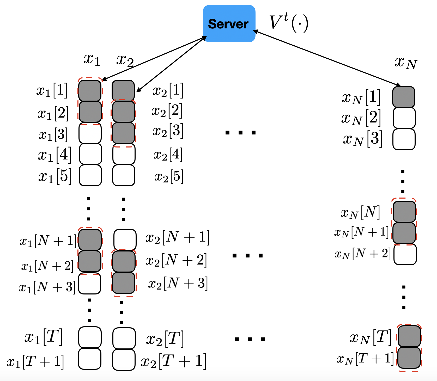
See Fig. 3 for an illustration of the construction discussed above.
Further, for a given error constant and a given the Lipschitz constant , let us define
| (25) |
Therefore, we also have
| (26) |
B.3 Properties.
First we present some properties of the component functions ’s.
Lemma 1.
The functions and satisfy the following:
-
1.
For all , , .
-
2.
The following bounds hold for the functions and their first- and second-order derivatives:
-
3.
The following key property holds:
(27) -
4.
The function is lower bounded as follows:
-
5.
The first-order derivative of (respectively, ) is Lipschitz continuous with constant (respectively, , ).
Proof. Property 1) is easy to check.
To prove Property 2), note that following holds for :
| (28) |
Obviously, is an increasing function over , therefore the lower and upper bounds are ; is increasing on and decreasing on , where , therefore the lower and upper bounds are ; is decreasing on and increasing on (this can be verified by checking the signs of in these intervals). Therefore the lower and upper bounds are , i.e.,
Further, for all , the following holds:
| (29) |
Similarly, as above, we can obtain the following bounds:
To show Property 3), note that for all and ,
where the first inequality is true because is strictly increasing and is strictly decreasing for all and , and that .
Next we show Property 4). Note that and . Therefore we have and using the construction in (22)
| (30) | ||||
| (31) |
where the first inequality follows from , the second follows from , and the last is true because .
Finally, we show Property 5), using the fact that a function is Lipschitz if it is piecewise smooth with bounded derivative. Before proceeding, let us note a few properties of the construction in (24) (also see Fig. 3). First, for a given node , its local function is only related to the following ’s
or equivalently
Then the first-order partial derivative of can be expressed below.
Case I) If we have
| (32) |
Case II) If , we have
| (33) |
From the above derivation, it is clear that for any , is either zero or is a piecewise smooth function separated at the non-differentiable point , because the function is not differentiable at .
Further, fix a point and a unit vector where . Define
to be the directional projection of on to the direction at point . We will show that there exists such that for all (where the second-order derivative is taken with respect to ).
First, by noting the fact that each if appears in , then it must also be coupled with either or , but not other ’s for . This means that , . Using this fact, we can compute as follows:
where we take and .
By using (32) and the above facts, the second-order partial derivative of () is given as follows when :
| (34) |
| (35) |
| (40) |
By applying Lemma 1 – i) [i.e., for ], we can obtain that at least one of the terms or is zero. It follows that
Taking the maximum over equations (34) to (40) and plug in the above inequalities, we obtain
where the equality comes from Lemma 1 – ii).
Summarizing the above results, we obtain:
Overall, the first-order derivatives of are Lipsschitz continuous for any with constant at most .
The following lemma is a simple extension of the previous result.
Lemma 2.
-
1.
We have
-
2.
We have
(41) -
3.
The first-order derivatives of and that for each are Lipschitz continuous, with the same constant .
Proof. To show that property 1) is true, note that we have the following:
Then by applying Lemma 1 we have that for any , the following holds
Property 2) is true is due to the definition of , so that we have:
Property 3) is true because the following:
where the last inequality comes from Lemma 1 – (5). This completes the proof.
Next let us analyze the size of . We have the following result.
Lemma 3.
If there exists such that , then
Proof. The first inequality holds for all , since is one element of . We divide the proof for the second inequality into two cases.
Case 1. Suppose for all . Therefore, we have . Using (33), we have the following inequalities:
| (42) |
where is true because are all non-negative from Lemma 1 -(2); is true due to Lemma 1 – (3). Therefore, we have the following
Case 2) Suppose there exists such that .
We choose so that and . Therefore, depending on the choices of we have three cases:
| (43) |
First, note that , for all , by checking the definitions of .
Then for satisfying the first condition, because and , using Lemma 1 – (3), and the fact that the negative part is zero for , and is even function, the expression further simplifies to:
| (44) |
If the second condition holds true, the expression is obviously non-positive because both and are non-negative. Overall, we have
This completes the proof.
Lemma 4.
Consider using an algorithm of the form (20) to solve the following problem:
| (45) |
Assume the initial solution: . Let denote some linear combination of local variables, where are the coefficients (possibly time-varying and dependent on ). Then no matter how many local computation steps (20b) are performed, at least communication steps (20a) are needed to ensure .
Proof. For a given , suppose that , , that is, for all . Then for all , and has the following partial derivative (see (32))
| (46) | ||||
| (47) |
Clearly, if , then by the definition of , the above partial gradient is also zero. In other words, the above partial gradient is only non-zero if .
Recall that we have assumed that the server aggregation is performed using a linear combination , with the coefficients ’s possibly depending on the stage (but such a dependency will be irrelevant for our purpose, as will be see shortly). Therefore, at a given stage , for a given node , when , its th element will become nonzero only if one of the following two cases hold true:
-
•
If before the aggregation step (i.e., at stage ), some other node has being nonzero.
-
•
If is nonzero at stage .
Now suppose that the initial solution is for all . Then at the first iteration only is non-zero for all , due to the fact that for all from (33). It is also important to observe that, if all nodes were to perform subsequent local updates (20b), the local variable will have the same support (i.e., only the first element is non-zero). To see this, suppose , then for , we have
| (48) |
since implies . Similarly reasoning applies when , .
If , then these local functions are not related to , so the partial derivative is also zero.
Now let us look at node . For this node, according to (46), we have
| (49) |
Since can be non-zero, then this partial gradient can also be non-zero. Further, with a similar argument as above, we can also confirm that no matter how many local computation steps that node performs, only the first two elements of can be non-zero.
So for the first stage , we conclude that, no matter how many local computation that the nodes perform (in the form of the computation step given in (20b)), only can have two non-zero entries, while the rest of the local variables only have one non-zero entries.
Then suppose that the communication and aggregation step is performed once. It follows that after broadcasting to all the nodes, everyone can have two non-zero entries. Then the nodes proceed with local computation, and by the same argument as above, one can show that this time only can have three non-zero entries. Following the above procedure, it is clear that each aggregation step can advance the non-zero entry of by one, while performing multiple local updates does not advance the non-zero entry. Then we conclude that we need at least communication steps, and local gradient computation steps, to make possibly non-zero.
B.4 Main Result for Claim 2.1.
Below we state and prove a formal version of Claim 2.1 given in the main text.
Theorem 2.
Let be a positive number. Let for all , and all . Consider any algorithm obeying the rules given in (10), where the and ’s are linear operators. Then regardless of the number of local updates there exists a problem satisfying Assumption 1 – 2, such that it requires at least the following number of stages (and equivalently, aggregation and communications rounds in (20a))
| (50) |
to achieve the following error
| (51) |
Proof of Claim 2.1. First, let us show that the algorithm obeying the rules given in (20) has the desired property. Note that the difference between two rules is whether the sampled local gradients are used for the update, or the full local gradients are used.
By Lemma 4 we have for all . Then by applying Lemma 2 – (2) and Lemma 3, we can conclude that the following holds
| (52) |
where the second inequality follows that there exists such that , then we can directly apply Lemma 3.
The third part of Lemma 2 ensures that ’s are -Lipschitz continuous gradient, and the first part shows
Therefore we obtain
| (53) |
This completes the proof.
Second, consider the algorithm obeying the rules give in (10), in which local sampled gradients are used. By careful inspection, the result for this case can be trivially extended from the previous case. We only need to consider the following local functions
| (54) |
where each sampled loss function is defined as
| (55) |
where ’s satisfy and . It is easy to see that, the local sampled gradients have the same dependency on as their averaged version (by dependency we meant the structure that is depicted in Fig. 3). Therefore, the progression of the non-zero pattern of the average is exactly the same as the batch gradient version. Additionally, since the local function is exactly the same as the previous local function , so other estimates, such as the one that bounds , also remain the same.
Appendix C Proof of Claim 2.2
First let us consider FedAvg with local-GD update (9). We consider the following problem with , which satisfies both Assumptions 1 and 2, with
| (56) |
Each local iteration of the FedAvg is given by
| (57) |
For simplicity, let us define , and define the matrix . Then running rounds of the FedAvg algorithm starting with for some non-negative integer , can be expressed as
| (58) |
Therefore overall we have
| (59) |
It is easy to show that for any , the eigenvalues of the matrix are and .
It follows that the above iteration will diverge for any starting from any non-zero initial point.
Moreover, when the sample on one agent are the same (e.g., agent 1 has two samples that both has loss function ), then using SGD as local update will be identical to the update of GD.
Appendix D Results showing the role of GB for FedAvg with diminishing stepsizes
This section is used to show the role of A3 in FedAvg. First we prove that with A3, FedAvg can use arbitrary stepsize as long as it diminishes to zero. Next, we show by a simple example that without A3, FedAvg will diverge with the same diminishing stepsize choice.
Claim D.1.
Claim D.2.
Before we prove Claim D.1, the following lemma is needed.
Lemma 5.
Proof: By using A1 we have:
| (61) | ||||
where comes from the update rule in Algorithm 1, in we use Jensen’s inequality and notice so in we extract the terms with index from the inner product.
Note that for any vector of the same length, the equality holds, we have
| (62) | ||||
where we use Jensen’s inequality in and A1 in .
Further note that
| (63) | ||||
The first equality comes from the update rule of , which basically performs steps of updates on ; comes from Jensen’s inequality; in we use A3.
Substitute (63) to (62) and then to (61), rearrange the terms we obtain (60), which ends the proof of the lemma.
D.1 Proof of Claim D.1
Next we prove Claim D.1
Proof: By choosing as constant and then applying Lemma 5 we have
| (64) | ||||
where . Using telescope sum from to we have
| (65) | ||||
Rearrange the terms and multiply both side by , then we have
| (66) | ||||
Choose , then . Choose as a sequence that diminishes to , then for all , as , . Therefore the right hand side converges to 0, Claim D.1 is proved.
Appendix E Proof of Claim D.2
Proof. We consider the following problem with , which satisfies both Assumptions 1 and 2, with
| (67) |
Each local iteration of the FedAvg is given by
| (68) |
For simplicity, let us define , and define the matrix . Then running rounds of the FedAvg algorithm starting with for some non-negative integer , can be expressed as
| (69) |
Therefore overall we have
| (70) |
In particular, we pick when and . Then for , it is easy to compute the eigenvalues of the matrix to be:
It is clear that is strictly larger than one which indicates that the algorithm will diverge.
Appendix F Proofs for Results in Section 3
F.1 Proof of Theorem 1
First let us prove Theorem 1 about the FedPD algorithm with Oracle I.
Towards this end, let us first introduce some notations. First recall that when Oracle I is used, the local problem is solved such that the following holds true:
| (71) |
Note that if SGD is applied in Oracle I to solve the local problem, then this condition (71) is replaced with the following
| (72) |
The difference does not significantly change the proofs and the results. So throughout the proof of Theorem 1, we use (71) as the condition.
Throughout the proof, we denote the expectation taken on the communication iteration to the iteration conditioning on all the previous knowledge as .
Then we define the error between different nodes as
| (73) |
Here, denotes the maximum difference of estimated center model among all the nodes and denotes the maximum difference of local models among all nodes.
From the termination condition that generates (given in (71)), we have
| (74) |
where the first equality holds because of the update rule of . Furthermore, from the update step of , we can explicitly write down the following expression
The first lemma shows the sufficient descent of the local AL function.
Lemma 6.
Then we derive a key lemma about how the error propagates if the communication step is skipped.
Lemma 7.
Suppose A1 and A5 hold. Consider FedPD with Algorithm 4 (Oracle I) as the update rule. When the local problem is solved such that (71) is satisfied, the difference between the local models ’s and the difference between local copies of the global models ’s are bounded by
| (76) |
where
is a rank matrix with eigenvalues and .
We define a virtual sequence where which is the average of the local and we know that when , that is, when the communication and aggregation step is performed. Next, we bound the error between the local AL and the global AL evaluated at the virtual sequence.
Lemma 8.
Lastly we bound the original objective function using the global AL.
Lemma 9.
Using the previous lemmas, we can then prove Theorem 1.
F.1.1 Proof of Lemma 6
We divide the left hand side (LHS) of (75), i.e., , into the sum of three parts:
| (79) | ||||
which correspond to the three steps in the algorithm’s update steps.
We bound the first difference by first applying A1 to :
and obtain the following series of inequalities:
| (80) | ||||
In the above equation, in we use the fact that when vector has the same length to the last two terms; in we split the last term into and ; in we use the fact that ; in we apply the fact that is the inexact solution; see (74).
Then we bound the second difference in (79) by the following:
| (81) | ||||
where directly comes from the update rule of .
F.1.2 Proof of Lemma 7
First we derive the relation between for arbitrary and by using the definition of (74):
| (83) | ||||
where in we plug the definition of and ; in we use A1; comes form A5; in we move the second term to the left and divide both side by .
Then we bound the difference by plugging in the expression of in (74), and note that :
| (84) | ||||
where and follow the same argument in , and of (83) ; in we plug in the definition of .
Next we bound the difference . With probability the aggregation step has just been done at iteration , .With probability , they are not equal, then we take expectation with communication probability , and get
| (85) | ||||
where in we plug in the definition of and (84). As these relations hold true for arbitrary pairs, they are also true for the maximum of and .
| (86) | ||||
Rewrite it into matrix form then we complete the proof of Lemma 7.
F.1.3 Proof of Lemma 8
| (87) | ||||
where follows the same argument in (82); in ,we plug in the definition of ; in we use Jensen’s inequality and we bound the term with . Then the lemma is proved.
F.1.4 Proof of Lemma 9
Applying A1, we have
| (88) | ||||
Taking an average over agents we are able to prove Lemma 9.
F.1.5 Proof of Theorem 1
First notice that from the optimality condition (74), the following holds:
| (89) |
Then we bound the gradients of .
| (90) | ||||
Further, we note that, when no aggregation has been performed at iteration , then , so the following holds
| (91) |
When there the aggregation has been performed at iteration , then , so we have
| (92) |
Further we have:
| (93) | ||||
| (94) |
Squaring both sides of the above inequality, we obtain:
| (95) |
where .
| (96) | ||||
Notice that when communication is not performed , and when communication is performed
| (97) | |||
where the last inequality holds due to the use of Jensen’s inequality, and the definition of in (73). It follows that summing both sides of (96) over , we have
| (98) | ||||
Taking the expectation over the randomness in , conditioning on the information before the communication the successive difference of ,
| (99) | ||||
where (a) expands the expectation on , and use the fact that with probability , , and with probability will be updated; in (b) we apply Lemma 8 to the last term.
| (100) | ||||
Next we bound the last term. By iteratively applying Lemma 7 from to and use the fact that , we have
| (102) |
| (103) | ||||
From the initial conditions we have and apply Lemma 9 we obtain
Finally we bound by
Therefore Theorem 1 is proved. During the proof, we need all , therefore, .
Finally, let us note that if the local problems are solved with SGD, then the local problem needs to be solved such that the condition (72) holds true. As no other information of the local solvers except error term is used in the proof, the proofs and results of FedPD with SGD as local solver will not change much, except that all the results hold in expectation. Therefore we skip the proof for the SGD version.
F.1.6 Constants used in the proofs
In this subsection we list all the constants used in the proof of Theorem 1.
we can see that when , all the terms are positive.
Appendix G FedPD with Variance Reduction
In this section we provided an alternative oracle for FedPD which has a lower sample complexity.
G.1 Algorithm description
Alternatively, when instantiating the local oracle using Algorithm 4, the original local problems are not required to solve to accuracy. Instead, we successively optimize a linearized AL function:
In the above expression, we linearize at inner iteration as ( is a constant)
where is an approximation of . The optimizer has a closed-form expression:
In Oracle II, an agent first decides whether to compute the full gradient , or to keep using the previous estimate . Then local steps are performed, each requires local data samples. In this scheme, can be chosen as any positive integer.
It is important to note that this oracle does not simply apply the VR technique (such as F-SVRG) to solve the subproblem of optimizing . That is, it is not a variation of Oracle I. Instead, the VR technique is applied to the entire primal-dual iteration, and the full gradient evaluation is only needed every iteration . Later we will see that if is large enough, then there is an reduction of sample complexity.
G.2 Algorithm Convergence and Complexity
The convergence result of FedPD with Oracle II is given as follows:
Theorem 3.
Remark 5. (Communication complexity): As , the communication round to achieve accuracy is which is independent of .
Remark 6. (Computation complexity): Note that the total number full gradient evaluation is , each uses samples. Meanwhile, the total number of mini-batch stochastic gradient evaluation is , each uses samples per node. So the total sample complexity is . In order to keep the same convergence speed, we need stepsize to be unchanged. Therefore, we choose , then the SC of Algorithm 4 is .
G.3 Proof of Theorem 3
Following the similar proof of Theorem 1, we first analyze the descent between each outer iteration. Notice throughout the proof, we assume that , that is, there is no delayed communication. It follows that the following holds:
We also recall that is the (outer) stage index, and is the local update index. First we provide a series of lemmas.
Lemma 10.
Then we deal with the variance of the stochastic gradient estimations.
Lemma 11.
Lastly we upper bound the original loss function.
Lemma 12.
G.3.1 Proof of Lemma 10
Let us first express the difference of the local AL as following:
| (108) | |||
where the above three differences respectively correspond to the three steps in the algorithm’s update steps.
Let us bound the above three differences one by one. First, note that we have the following decomposition (by using the fact that and ):
| (109) |
Each term on the right hand side (RHS) of the above equality can be bounded by (see a similar arguments in (80)):
| (110) | ||||
where in we use the optimal condition that which gives us the following relation
| (111) |
in we use the fact that . Therefore, the first difference in the RHS of (108) is given by
| (112) |
The other two differences in (108) can be explicitly expressed as:
| (113) | |||
| (114) |
Next we bound . Notice that the from the update rule the following holds:
| (115) |
Using the above property, we have
| (116) | ||||
where in we apply Cauchy-Schwarz inequality. Next we bound by
where in and we both apply Cauchy-Schwarz inequality, in we use A1 to the last term and in we notice .
which complete the proof of Lemma 10.
G.3.2 Proof of Lemma 11
To study , we denote the latest iteration before that computes full gradients as . That is, in we have . By the description of the algorithm we know
That is, is a multiple of and there is no more than local update steps between step and step . By the update rule of , we have
| (117) |
Take expectation on both sides, we have
By using the fact that and substitute (G.3.2) we have
where comes form the fact that we view as and by identically random sampling strategy we have and , in we use A1.
Iteratively taking expectation until , we have
| (118) |
which completes the proof.
G.3.3 Proof of Lemma 12
Applying A1, we have
G.3.4 Proof of Theorem 3
By the update step of , following (91) we have
We also have
where in , the first term is obtained by plugging in (115) given below
Taking expectation of (10), summing over to and average over the agents, we have the following
| (121) | ||||
Finally, in the last equation of (121), we have defined the constant as
Then by taking expectation and applying Lemma 12, we obtain
where by the initialization that we have
Combine (G.3.4) and (LABEL:eq:th_VR_2), we can find a positive constant satisfying
| (122) |
where we have defined
| (123) |
so that the following holds
| (124) | ||||
During the prove we need
to be positive constant. By selecting , and , this is guaranteed.
Appendix H Additional Numerical Results
H.1 Penalized Logistic Regression
In this experiment, we consider the penalized regression problem [30], whose loss function evaluated on a single sample is given by:
| (125) |
Here denotes the component of . The feature vector and model parameter have dimension and is the label corresponding to the feature. During the simulation, we set the constants to be and .
In the experiment, we use two ways to generate the data. In the first case (referred to as the “weakly non-i.i.d” case), the features and the labels on the agents are randomly generated, so the local data sets are not very non-i.i.d. In the second case (referred to as the “strong non-i.i.d.” case), we first generate the feature vector ’s following the standard Normal distribution, then we generate the local model on the agent by using uniform distribution in the range of for each component. Then we compute the label ’s according to the local models and the features and add some uniform noise. In this case, the data distribution on the agents are more non-i.i.d. compared to the first case. In both cases, there are samples on each agent with total agents.
The total number of iterations is set as for all algorithms. We choose the stepsize to be for FedAvg-GD with local update number and for FedAvg-SGD we use diminishing stepsize with . For FedProx we use VR algorithm as the local solver and set , and stepsize . For FedPD, we also use the same stepsize with with local GD. For FedPD-SGD, we also set and uses local step size with inner iteration number . Lastly for FedPD with VR, we set the parameters to be , , , and . The choice of the stepsize is the same among all the algorithms. We used grid search on stepsizes and the relative performance of the algorithms are similar to what we will show shortly.

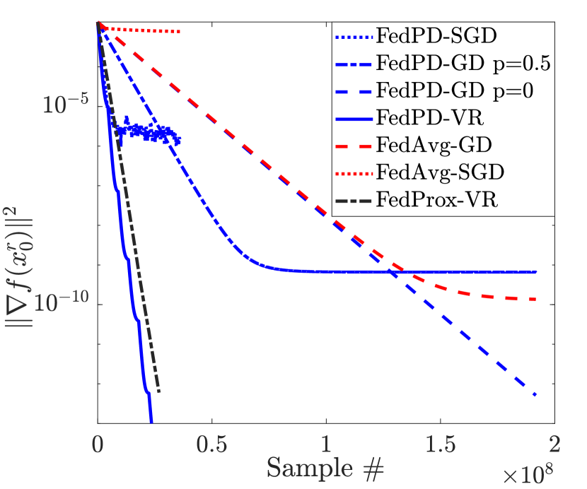
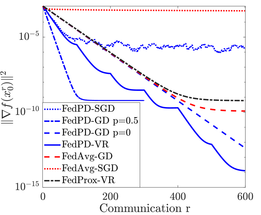
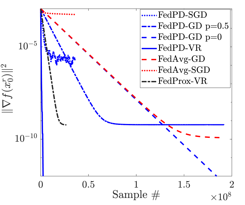
Fig. 4 shows the convergence results of the penalized logistic regression problem with the first data set. In Fig. 4(a), we compare the convergence of the tested algorithms w.r.t the communication rounds. It is clear that FedProx and FedPD with (i.e., no communication skipping) are comparable. Meanwhile, FedAvg with local GD will not converge to the stationary point with a constant stepsize when local update step . By skipping half of the communication, FedPD with local GD can still achieve a similar error as FedAvg, but using fewer communication rounds. In Fig. 4(b), we compare the sample complexity of different algorithms. It can be shown that when using the same number of samples for computation, FedPD with Oracle II (FedPD-VR) converges the fastest among all the algorithms. FedProx uses VR to solve the inner problem and converges the second fastest. Fig 5 shows the convergence results with the strongly non-i.i.d. data set. We can see that the algorithms using stochastic solvers become less stable compared with the case when the data sets are weakly non-i.i.d. Further, FedPD-VR and FedPD-GD with are able still to converge to the global stationary point while FedProx will achieve a similar error as the FedAvg with local GD.
H.2 Handwritten Character Classification
In the second experiment, we compare FedPD with FedAvg and FedProx on the FEMNIST data set [31]. The FEMNIST data set collects the handwritten characters, including numbers 1–10 and the upper- and lower-case letters A–Z and a–z, from different writers and is separated by the writers, therefore the data set naturally preserves non-i.i.d-ness.
The entire data set contains 805,000 samples collected from 3,550 writers. In our experiments, we use the data collected from 100 writers with an average of 300 samples per writer and the size of the whole data set is 29,214. We set the number of agent , the first ten agents are assigned with data from two writers, and the rest of the agents are assigned with data form one writer. Therefore, the data distribution is neither i.i.d. nor balanced. We use the neural network given in [31] as the training model, which consists of 2 convolutional layers and two fully connected layers. The output layer has 62 neurons that matches the number of classes in the FEMNIST data set.
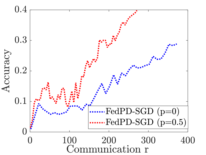
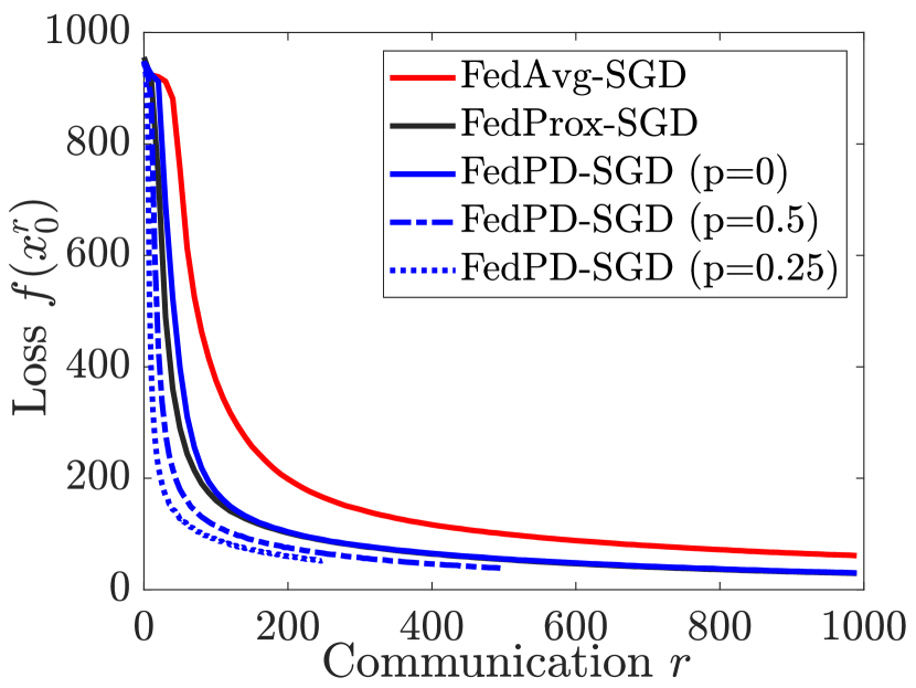
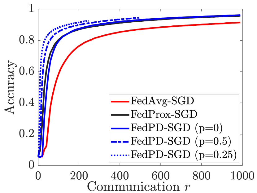
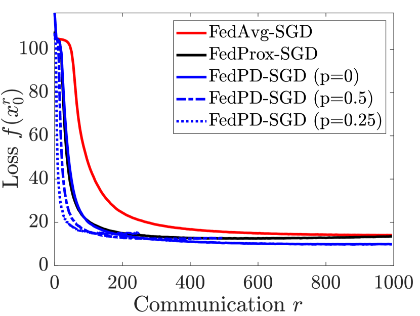
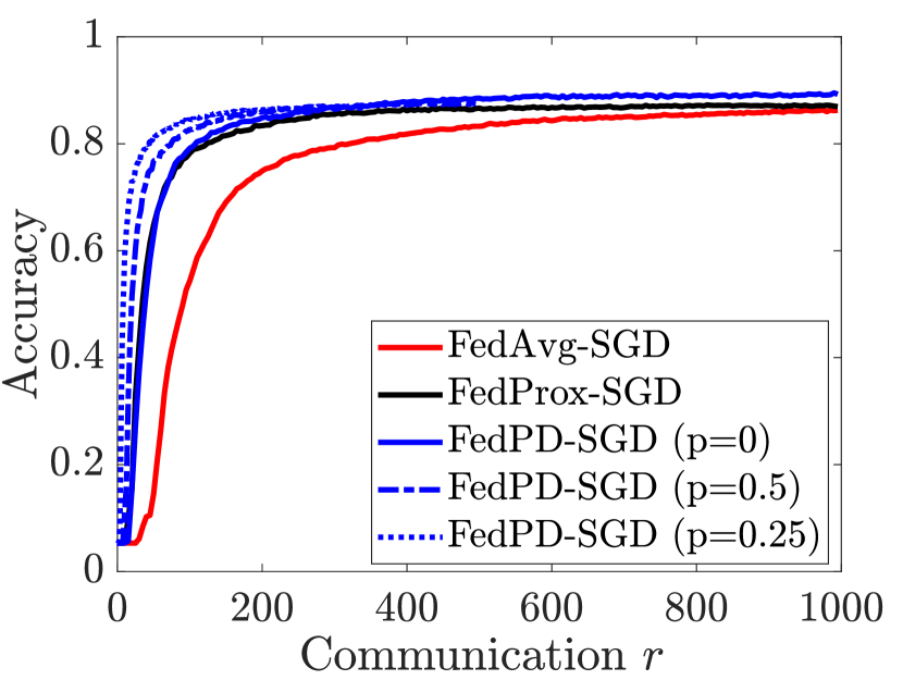
The numerical results shown in Fig. 6 in the main text were generated by running MATLAB codes on Amazon Web Services (AWS), with Intel Xeon E5-2686 v4 CPUs. In the training phase, we train the CNN model with FedAvg, FedProx and FedPD. In Fig. 6(a), for FedAvg, we use gradient descent for local update steps between each communication rounds; to solve the local problem for FedProx, we use SARAH with local steps; we use FedPD with Oracle II, computing full gradient every communication rounds and perform local steps between two communication rounds. The hyper-parameters we use for FedAvg is ; for FedProx we use and stepsize ; for FedPD we use and . In Fig. 6(b), we use FedPD with Oracle I, with , and and the mini-batch size . We set the communication saving to and .
The results shown in Fig. 7 were generated by running Python codes (using the the PyTorch package 111PyTorch: An Imperative Style, High-Performance Deep Learning Library, https://pytorch.org/) with AMD EPYC 7702 CPUs and an NVIDIA V100 GPU.
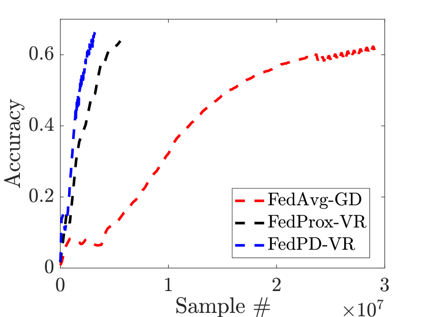
In the training phase, we train with FedProx, FedAvg and FedPD with a total outer iterations. The local problems are solved with SGD for local iterations and the mini-batch size in evaluating the stochastic gradient is . The stepsize choice for FedAvg, FedProx and FedPD are , and , the hyper-parameter of FedProx is and for FedPD . In the experiment, we set the communication saving for FedPD to be , and . Note that we also tested FedAvg with larger stepsize , but the algorithm becomes unstable, and its performance degrages significantly. As shown in Fig. 7 and 8, FedAvg is slower than FedPD and FedProx, while FedProx has similar performance as FedPD when . Further, we can see that as the frequency of communication of FedPD decreases, the final accuracy decreases and the final loss increases. However, the drop of accuracy is not significant, so FedPD is able to achieve a better performance with the same number of communication rounds.