Atom interferometry with thousand-fold increase in dynamic range

Abstract

The periodicity inherent to any interferometric signal entails a fundamental trade-off between sensitivity and dynamic range of interferometry-based sensors. Here we develop a methodology for significantly extending the dynamic range of such sensors without compromising their sensitivity, scale-factor, and bandwidth. The scheme is based on operating two simultaneous, nearly-overlapping interferometers, with full-quadrature phase detection and with different but close scale factors. The two interferometers provide a joint period much larger than $2\pi$ in a moiré-like effect, while benefiting from close-to-maximal sensitivity and from suppression of common-mode noise. The methodology is highly suited to atom interferometers, which offer record sensitivities in measuring gravito-inertial forces but suffer from limited dynamic range. We experimentally demonstrate an atom interferometer with a dynamic-range enhancement of over an order of magnitude in a single shot and over three orders of magnitude within a few shots, for both static and dynamic signals. This approach can dramatically improve the operation of interferometric sensors in challenging, uncertain, or rapidly varying, conditions.

The ambiguity-free dynamic range of interferometric physical sensors is fundamentally limited to $2\pi$ radians. When the a priori phase uncertainty is larger than a single fringe, additional information is required to uniquely determine the physical quantity measured by the interferometer. If this quantity remains constant over long periods of time, the phase ambiguity may be resolved through additional interferometric measurements with different scale-factors, defined as the ratio between the interferometer phase and the magnitude of the physical quantity. A more challenging scenario arises when the physical quantity changes rapidly with time, and measurement with multiple scale-factors must be realized simultaneously.

Overcoming this challenge in cold-atom interferometers (Tino and Kasevich, 2014), which have emerged over the past decades as extremely sensitive sensors of gravitational and inertial forces, is an especially ambitious proposition. Applications of atom interferometers vary from fundamental research (Müller et al., 2010; Kovachy et al., 2015; Barrett et al., 2016; et al., 2018; Xu et al., 2019) and precision measurements (Rosi et al., 2014; Parker et al., 2018) to gravity surveys and inertial navigation (Geiger et al., ). Mobile interferometers are being developed by several groups (Bongs et al., 2019; Farah et al., 2014; Freier et al., 2016; M.énoret et al., 2018) with demonstrations of land-based, marine, and airborne gravity surveys (Bidel et al., 2018; Wu et al., 2019; Bidel et al., 2020).

In these applications, limited dynamic range is especially challenging, as the uncertainty in the acceleration to be measured is potentially very large. Reducing the interferometer scale-factor or performing multiple measurements at each location results in reduced sensitivity or lower temporal bandwidth, respectively. A common solution relies on auxiliary sensors with larger dynamic range but lower resolution to constrain the interferometric measurement to a smaller, non-ambiguous range (Merlet et al., 2009; Lautier et al., 2014). However, this approach may suffer from transfer-function errors, misalignment between the sensors, or non-linearities (Bidel et al., 2018). It is therefore highly desirable to have a high-sensitivity, high-bandwidth, atom interferometer with a large dynamic range. While optical interferometers may gain such capabilities by employing and detecting multiple wavelengths (Dändliker and Salvadé, 1999; Falaggis et al., 2009), this feat is more challenging for matter-wave interferometers.

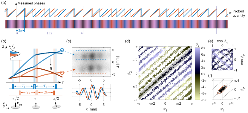
In this work, we achieve a dramatic enhancement of dynamic range on a single-shot basis by combining two powerful approaches in atom interferometry: increasing the dynamic range without sensitivity loss through small variations of the interferometer scale factor (Avinadav et al., 2020a), and acquiring multiple phase measurements in a single experimental run (Bonnin et al., 2018; Yankelev et al., 2019). First, when the same fundamental physical quantity determines two interferometric phases with slightly different scale factors, it can be uniquely extracted within an enhanced dynamic range, determined by a moiré wavelength which is inversely proportional to the difference between scale-factors [Fig. 1(a)]. Second, by operating and reading out the two interferometers simultaneously within the same experimental shot, major common-mode noises are rejected, increasing the scheme’s robustness to dominant sources of noise. Additionally, such operation maintains the original temporal bandwidth of the measurement. Further exponential increase in dynamic range, at the cost of a linear reduction of temporal bandwidth, is achieved by varying the scale-factor ratio between shots.

Figure 1: Concept, scheme and results of dual-$T$ interferometry. (a) Conceptual representation of dynamic-range enhancement by a factor of $\times 8$, using a pair of simultaneous interferometers with different scale factors. (b) Dual-$T$ atom interferometry. A pair of Raman pulse sequences (red and blue), with different interrogation times $T$ and addressing different velocity classes of the atoms, couple between two atomic states with momentum difference of $\hbar k_{\textrm{eff}}$ (bright and dark trajectories). To obtain full phase quadrature information, the Raman retro-reflecting mirror is tilted before the final $\pi/2$ pulses, generating a transverse phase gradient across the cloud. (c) Top: a single fluorescence image captures the population in one of the atomic states for both interferometers. Bottom: measured cross-sections (solid lines) and the fitted fringes (dashed lines) of both interferometers, after vertical integration of the regions indicated by the dashed rectangles and subtraction of the Gaussian envelope. The interferometer phases $\phi_{1},\phi_{2}$ are determined by the fringe phase at the center of each cloud. (d) Results of dual-$T$ interferometry for inertial phase $\phi_{a}$ in the range of $\pm 8\pi$ (color coded), each dot represents a single dual-$T$ measurement. Slope of gray lines is the scale-factor ratio $\tau=\left(T_{2}/T_{1}\right)^{2}=7/8$. Shaded region represents the original, ambiguity-free, $2\pi$ dynamic range of a single interferometer operated at $T=T_{1}$. Full-quadrature phase-detection allows for a unique solution for all phases, compared to ambiguities generated when detecting only the cosine component (e). (f) Dual-$T$ measurements at constant inertial phase $\phi_{a}=0$, demonstrating that the noise in both interferometers is highly correlated with slope $\sim\tau$. In red, the covariance ellipse at 95% confidence level.

Principles of Dual-$T$ Interferometry

We realize the above concept in a Mach-Zehnder atom interferometer measuring the local acceleration of gravity (Kasevich and Chu, 1991). Such devices use light-pulses as “atom-optics” that split the atomic wavepacket into two ams and later recombine them after they traveled on macroscopically distinct trajectories. The differential phase accumulated between the arms of the interferometer depends on the motion of the atoms.

In our experiment, laser-cooled ${}^{87}\textrm{Rb}$ atoms are launched vertically on a free-fall trajectory. Counter-propagating, vertical laser beams at $780\,\mathrm{nm}$ drive two-photon Raman transitions between two electronic ground states while imparting recoil of two photon momenta (Kasevich et al., 1991). The Raman beams are sent from the top and are retro-reflected from a stabilized mirror at the bottom, which defines the reference frame with respect to which the motion of the atoms is measured. The interferometric sequence is composed of three Raman pulses, equally spaced by time $T$, acting to split the atomic wavepacket into two components that drift apart, and then to redirect and recombine them, leading to a final atomic population ratio determined by the phase difference between the two arms.

In this configuration, the phase difference is determined by the gravitational acceleration $g$ according to $\phi_{a}=\left(k_{\textrm{eff}}g-\alpha\right)T^{2}$, with $\hbar k_{\textrm{eff}}$ the total momentum transferred by the Raman interaction, and $\alpha$ a chirp rate applied to the relative frequency between the Raman beams to compensate for the changing Doppler shift of the falling atoms. Residual vibrations of the mirror contribute noise to the inertial phase $\phi_{a}$.

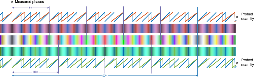
The concept we develop relies on a so-called dual-$T$ operation of the interferometer. Instead of one pulse sequence, two interleaved pulse sequences with slightly different $T$ values are performed [Fig. 1(b)]. By tuning their two-photon Doppler-detunings, each set of pulses addresses a different vertical velocity class of the atoms. We operate the two interferometers with scale factors differing by the ratio $\tau\lesssim 1$, choosing the interferometric durations $T_{1}=T$ and $T_{2}=\sqrt{\tau}T$, with $T=55\,\mathrm{ms}$ (see Methods).

Figure 2: Analysis of dual-$T$ interferometry measurements in single-shot, two-shot, and three-shot operation. (a) Single-shot dual-$T$ operation with $D=8$ for $\phi_{a}$ in the range of $\pm 8\pi$ (color coded). Every dot corresponds to a single measurement. Each discrete value of $\phi_{\textrm{diff}}$ corresponds to a different sub-range of $\phi_{a}$, and within that sub-range $\phi_{\textrm{sum}}$ changes continuously and linearly with $\phi_{a}$. (b) Sequential two-shot dual-$T$ operation with $D=7,8$ for $\phi_{a}$ in the range of $\pm 56\pi$, presented in the $\phi_{\textrm{diff}}^{\left(D=7\right)}$-$\phi_{\textrm{diff}}^{\left(D=8\right)}$ plane. The discrete clusters in this plane correspond to different sub-ranges of $\phi_{a}$. (c) Sequential three-shot dual-$T$ operation with $D=5,7,8$ for $\phi_{a}$ in the range of $\pm 280\pi$, presented in the $\phi_{\textrm{diff}}^{\left(D=5\right)}$-$\phi_{\textrm{diff}}^{\left(D=7\right)}$-$\phi_{\textrm{diff}}^{\left(D=8\right)}$ space. For clarity, only a subset of the solutions around $\phi_{\textrm{diff}}^{(D=5,7,8)}=0$ is presented, and gray ovals surround the expected solutions.

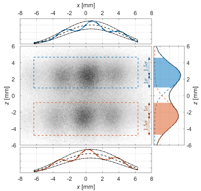
Conventionally, the population ratio between the interferometer states is measured directly, and the cosine of the phase is extracted. In our dual-$T$ scheme, we detect the phases $\phi_{1},\phi_{2}$ of both interferometers by acquiring an image of the atoms in one of the final atomic states. The independent readout of both interferometers is enabled by the ballistic expansion of the cloud, which maps the different velocity classes onto different vertical positions. To obtain the phase, in a manner equivalent to full quadrature detection where both sine and cosine components of the phase are measured, we use phase-shear readout (Sugarbaker et al., 2013). We tilt the retro-reflecting Raman mirror by a small angle before the final $\pi/2$-pulses to generate a spatial transverse interference pattern across the cloud, as utilized in point-source interferometry (Dickerson et al., 2013; Chen et al., 2019; Avinadav et al., 2020b) and shown in Fig. 1(c). The phase offset of this pattern can be directly extracted with constant sensitivity for all interferometric phases.

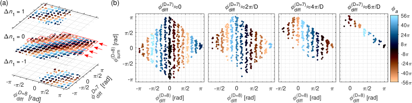
Figure 1(d) shows single-shot measurements in a dual-$T$ operation with the dynamic range enhanced by a factor of 8. We vary $\phi_{a}$ by changing the chirp rate $\alpha$ with respect to its nominal value $\alpha_{0}=k_{\textrm{eff}}g$, thereby emulating changes in $g$. We find that $\phi_{a}$ is mapped onto a unique set of straight, parallel lines in the plane spanned by $\phi_{1}$ and $\phi_{2}$ owing to the quadrature detection capability. Conversely, conventional detection which resolves only the cosine of the phase, would result in many phase ambiguities due to very different values of $\phi_{a}$ being mapped to similar measured phase components [Fig. 1(e)], severely limiting the benefits of a dual-$T$ operation. Quadrature detection, together with the strong suppression of common noise due to operation at very similar scale factors, allows the dual-$T$ scheme to achieve a significantly larger enhancement compared to past implementations of simultaneous atom interferometers with different scale factors (Bonnin et al., 2018).

Dual-$T$ Phase Analysis

Phase estimation for single shot dual-$T$. The measured interferometric phases $\phi_{1},\phi_{2}$ are constrained to the bare dynamic range $\pm\pi$ and can be written as

$$\phi_{1} =\phi_{a}-2\pi n_{1},$$ (1)

$$\phi_{2} =\tau\phi_{a}-2\pi n_{2}.$$ (2)

The integers $n_{1}$ and $n_{2}$, which respectively bring $\phi_{1}$ and $\phi_{2}$ to the range $\pm\pi$, are a priori unknown.

We define $D\equiv\left(1-\tau\right)^{-1}$, with $\tau=\left(T_{2}/T_{1}\right)^{2}$ the scale-factors ratio. For integer values of $D$, the dynamic-range enhancement is exactly $D$; as illustrated in Fig. 1(a), $\phi_{1}$ and $\phi_{2}$ have a joint period of $2D\pi$ as in a moiré effect, resulting in an extended ambiguity-free dynamic range of $\pm D\pi$ (see Methods for discussion on non-integer values).

Figure 3: Performance analysis of dual-$T$ interferometry. (a) Estimated inertial phase for single-shot measurements (left; inset shown zoom on $\pm\pi/2$ region) and for sequential two-shot (center) and three-shot (right) measurements, with dynamic range enhancement factors of $10$, $110$, and $990$, respectively. Outlying measurements appear as data points visibly distant ($>2\pi$) from their expected value. We observe only 10, 24, and 26 such outliers out of 2000 data points in the three data sets, respectively. (b) Residuals of the estimated phases, including only non-outlying measurements. Compared to single-shot measurements, standard deviations of two- and three-shot residuals are smaller by factors of $\sqrt{2}$ and $\sqrt{3}$, respectively. (c) Outlier probability $\epsilon$ as a function of dynamic range enhancement obtained for individual values of $D$ and for various combinations of consecutive coprime $D$ values. For $D\leq 8$, there were no outliers in the measured data set. Error bars represent 67% confidence intervals of the estimated value. Solid lines are calculated using Eq. (10) with $\sigma_{\textrm{ind}}=80\,\mathrm{mrad}$. Dashed lines represent outlier probability for an alternative scheme of averaging two or three sequential shots using a single $D$ value. (d) Estimation error of gravitation phase per shot $\sigma_{\phi,\textrm{est}}$. The error is dominated by vibration-induced phase noise and is nearly equal for all realizations. In (c),(d), arrows indicate the measurements shown in (a),(b).

To analyze a dual-$T$ measurement, we define the quantities $\phi_{\textrm{diff}}$ and $\phi_{\textrm{sum}}$,

$$\left(\begin{array}[]{c}\phi_{\textrm{diff}}\\ \phi_{\textrm{sum}}\end{array}\right) =\frac{1}{1+\tau^{2}}\left(\begin{array}[]{cc}\tau&-1\\ 1&\tau\end{array}\right)\left(\begin{array}[]{c}\phi_{1}\\ \phi_{2}\end{array}\right).$$ (9)

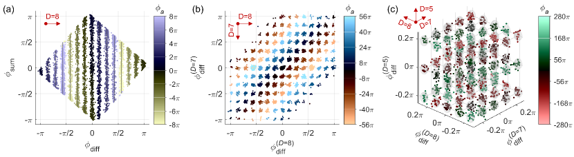
$\phi_{\textrm{diff}}$ and $\phi_{\textrm{sum}}$ act as coarse and fine measurements, respectively. As shown in Fig. 2(a), which presents an analysis of $D=8$ dual-$T$ measurements, $\phi_{\textrm{diff}}$ takes on a discrete set of $2D-1$ values. This constrain uniquely determines the values of $n_{1}$ and $n_{2}$ and hence the $2\pi$ sub-range in which $\phi_{a}$ lies. Correspondingly, $\phi_{\textrm{sum}}$ is a continuous variable, providing the estimation of the inertial phase $\phi_{a}$ within that sub-range (see Methods).

Phase estimation for sequential operation. We now turn to discuss further enhancement of dynamic range obtained by a sequence of several dual-$T$ shots with alternating integer values of $D$. Here we fix $T_{1}$ and alternate $T_{2}$ between shots. Assuming that changes in $\phi_{a}$ are small between consecutive shots, the above analysis per shot provides $n_{1}\,\text{mod}\,D$. Taken together, the full sequence uniquely determines $n_{1}$ within a range defined by the least common multiple of the employed $D$ values, or, for coprime integers, simply their product (see Methods and Fig. S1).

Analyses of two-shot operation with $D=7,8$ and three-shot operation with $D=5,7,8$ are shown in Fig. 2(b,c). Each data point is a measurement with a random value of $\phi_{a}$ within the extended dynamic ranges $\pm 56\pi$ and $\pm 280\pi$, respectively. We observe two- and three-dimensional clustering of the differential phases $\phi_{\textrm{diff}}$, where each cluster corresponds to a unique, non-ambiguous phase range smaller than $2\pi$.

Noise and outlier probability. By virtue of simultaneously operating the two interferometers with similar scale factors, vibrations-induced phase noise is highly correlated between them [Fig. 1(f)] and has negligible contribution to $\phi_{\textrm{diff}}$. The dominant noise in $\phi_{\textrm{diff}}$ results from uncorrelated, independent detection noise in $\phi_{1}$ and $\phi_{2}$, whose standard deviation we denote as $\sigma_{\textrm{ind}}$ (see Methods for a detailed discussion of noise terms).

As $D$ is increased, and the discrete values of $\phi_{\textrm{diff}}$ become denser, the uncorrelated noise may lead to errors in determining the correct sub-range for $\phi_{a}$, producing an outlier with phase estimation error in multiples of $2\pi$. The probability $\epsilon$ for a measurement to be such an outlier is approximately [see Eq. (16) for exact expression]

$$\epsilon\approx\mathrm{erfc}\left(\frac{\pi}{2}\frac{1}{D\cdot\sigma_{\textrm{ind}}}\right).$$ (10)

Crucially, $\epsilon$ depends only on the uncorrelated noise and not on the vibrations-dominated correlated noise, which is typically much larger. In the data presented in Fig. 2(a), we observe one such outlier out of 5000 measurements for $D=8$.

For the case of sequential dual-$T$ operation, the total outlier probability $\epsilon_{\textrm{seq}}$ depends on the outlier probabilities in each shot and, in the relevant regime of small error probabilities, is given simply by their sum. For any desired dynamic range and temporal bandwidth, the outlier probability is minimized by choosing consecutive coprime values of $D$.

Experimental Characterization

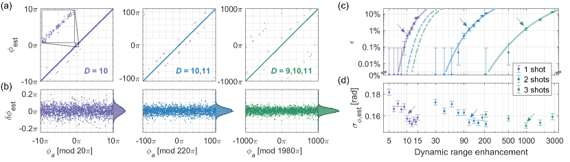
Performance analysis. To quantify the performance of the dual-$T$ scheme in terms of phase sensitivity and outlier probability, we extend the phase scan to random, known, values of $\phi_{a}$ within the range of $\pm 1000\pi$, corresponding to accelerations of $\pm 65\,\mathrm{mm/s^{2}}$ at $T=55\,\mathrm{ms}$. For each phase, we perform measurements with $D$ values between 5 and 15, and perform dual-$T$ analysis using each $D$ separately, using pairs of consecutive $D$ values, and using triplets of consecutive coprime $D$ values. We analyze each measurement within its appropriate extended dynamic range; data points that are outside the measurement’s relevant dynamic range are wrapped back onto it. We then compare the extracted phase to its expected value, from which we estimate the outlier probability $\epsilon$ as well as the phase residuals of the measurements without outliers.

The results, presented in Fig. 3, demonstrate an enhancement of dynamic range by factors of $10$ in a single shot, $\sim 100$ in two shots, and $\sim 1000$ in three shots, while maintaining phase residuals of $\sigma_{\textrm{$\phi,$est}}\sim 160\,\mathrm{mrad/shot}$ ($\sim 3.3\,\mathrm{\mu m/s^{2}/shot}$), and with outlier probabilities of 0.5%, 1.1%, and 1.2%, respectively. In general, we find excellent agreement with the error model described by Eq. (10), with $\sigma_{\textrm{ind}}=80\,\mathrm{mrad}$ estimated from these data.

We note that an outlier fraction on the order of 1% is acceptable in most applications, as such outliers can be identified and removed by comparison to adjacent shots or using auxiliary measurements. However, even if nearly zero outlier fraction is required, the dual-$T$ scheme can deliver a significant dynamic range enhancement. For example, with the above measured value of $\sigma_{\textrm{ind}}$ and for $D=6$, we expect $\epsilon\approx 3\times 10^{-6}$.

Furthermore, averaging over $N$ repeated measurements with the same $D$ value can decrease the outlier probability $\epsilon$ by effectively reducing $\sigma_{\textrm{ind}}$ by a factor $\sqrt{N}$. However, by employing the same number of sequential measurements with alternating values of $D$ as described above, the same value of $\epsilon$ may be achieved with significantly larger dynamic range enhancement, as seen from comparing solid and dashed curves in Fig. 3(c).

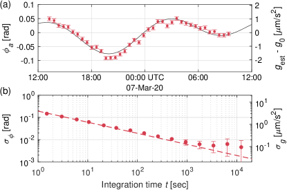
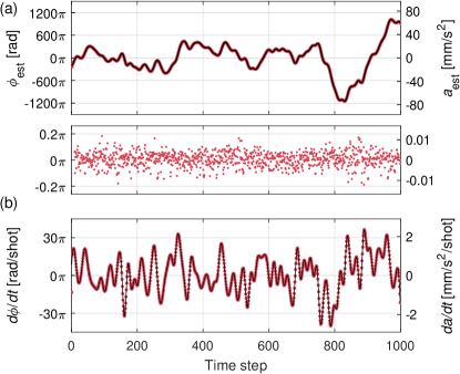
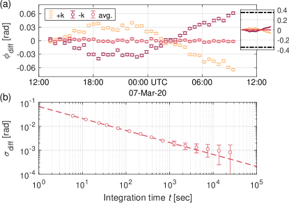
Stability of dual-$T$ interferometry. To demonstrate the long-term stability of dual-$T$ interferometry, we continuously measure gravity over 20 hours with $D=10$. As shown in Fig. 4, $\phi_{a}$ follows the expected tidal gravity variations throughout the measurement period. It remains stable at time scales of $10^{4}\,\mathrm{sec}$, to better than $100\,\mathrm{nm/s^{2}}$, showing that the dual-$T$ scheme does not add significant drifts to the estimated phase. Conversely, $\phi_{\textrm{diff}}$ does exhibit small drifts which we attribute to mutual light-shift between the two interferometers. However, due to the discrete nature of $\phi_{\textrm{diff}}$, these drifts can be easily corrected in several ways (see Methods).

Figure 4: Stability of dual-$T$ interferometry. (a) Time series of $\phi_{\textrm{sum}}$, with half-hour binning, measured with $D=10$. The results follow the expected tidal gravity variation as calculated from solid-earth model (black solid line). (b) Allan deviation of the residuals of $\phi_{\textrm{sum}}$ from the tidal model. Dashed line is a fit to $t^{-1/2}$ with sensitivity per shot of $155\,\mathrm{mrad}$ ($3.2\,\mathrm{\mu m/s^{2}}$).

Tracking fast-varying signals

We now turn to discuss dynamic scenarios, such as mobile gravity surveys or inertial measurements on a navigating platform, where the measured acceleration and thus $\phi_{a}$ change dramatically between shots. Dual-$T$ interferometry with fixed $D$ can directly track a signal that randomly varies by up to $\pm D\pi$ from shot to shot. Moreover, alternating the value of $D$ between consecutive measurements can enable tracking a signal with even larger variations; however, the sequential analysis described above cannot be applied due to the phase changing between shots, and a different analysis method is required.

Figure 5: Tracking of a time-varying acceleration using dual-$T$ interferometry combined with a particle-filter protocol. Measurements are performed with alternating $D=9,10$. (a) Acceleration signal extracted from the measurements using the particle filter (red), compared to the input signal (black). Bottom panel shows the residuals with standard deviation of $174\,\mathrm{mrad}$ ($3.6\,\mathrm{\mu m/s^{2}}$). (b) Temporal derivative (shot-to-shot variation) of the measured acceleration signal (red) compared to the input (black).

To track such a signal, we employ a particle filter estimation protocol (Moral, 1996; Merwe et al., 2001). Particle filtering is a powerful and well-established technique in navigation science, signal processing and machine learning, among other fields. It is a sequential, Monte-Carlo estimation approach based on a large number of particles which represent possible hypotheses of the system’s current state, e.g., the inertial phase measured by the sensor. These hypotheses are weighted through Bayesian estimation after every measurement, converging on a solution that is consistent with the sensor readings over time. In our context, under some model assumptions on the signal dynamics, use of particle filter enables full recovery of the single-shot bandwidth (Avinadav et al., 2020b) while maintaining the large increase in dynamic range rendered by the sequential operation.

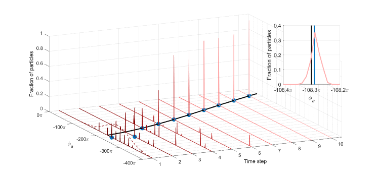
An experimental realization of tracking a dynamic signal is presented in Fig. 5. We change the chirp rate $\alpha$ between shots to simulate a band-limited random walk of $a$ and perform dual-$T$ measurements with alternating $D=9,10$. The sequence of measured phases is then analyzed with a particle filter protocol using a second-order derivative model (see Methods), to extract best estimate for the time-series of $\phi_{a}$. Following a brief convergence period (Supplementary Fig. S4), we successfully track this time-varying signal which spans over $2000\pi$ and changes by up to $40\pi$ between shots, with sensitivity per shot similar to measurements of static signals under similar conditions, and with no outliers. We note that while the analysis was carried out in post-process, it is in principle compatible with implementation as a real-time protocol.

Discussion

In conclusion, we present a novel approach to atom interferometry for significant enhancement of dynamic range without a reduction in sensitivity and with high measurement bandwidth. In applications where traditional atom interferometers must be operated at reduced sensitivity due to the expected dynamic range of the measured signal, our approach enables measurements with a substantial increase in sensitivity while maintaining the necessary dynamic range.

Taking advantage of full-quadrature phase detection and common-noise rejection, we experimentally demonstrate an increase of dynamic range by more than an order of magnitude in a single shot. Incorporating data from several consecutive shots, the dynamic range further increases in exponential fashion, allowing us to reach three orders of magnitude gain using only three measurements. Finally, we demonstrate tracking of a dynamical signal with tens of radians shot-to-shot variation by combining the dual-$T$ measurement with a particle-filter protocol, representing a major improvement compared to recent works (Avinadav et al., 2020a).

This approach can dramatically enhance performance of sensors, and in particular inertial-sensing atom interferometers, under challenging conditions, by enabling non-ambiguous operation without sacrificing either sensitivity or bandwidth. Such conditions are encountered in field operation of such sensors, for example in mobile gravity surveys or when used for inertial navigation on a moving platform. By extending the sensor real-time dynamic range, the requirements on vibration isolation or corrections based on auxiliary measurements can be relaxed, or equivalently, existing sensors can be operated in more demanding environments.

Dual-$T$ measurements can be realized by multiple means, based on known atom interferometry tools, e.g., dual-species interferometry (Bonnin et al., 2018) or momentum-state multiplexing (Yankelev et al., 2019), in addition to phase-shear readout (Sugarbaker et al., 2013) used in this work. It is also compatible with important atom-interferometry practices, such as $k$-reversal (McGuirk et al., 2002; Louchet-Chauvet et al., 2011) and zero-dead-time operation (Dutta et al., 2016). Further improvement of the scheme is possible by incorporating more than two interferometric sequences within the same experimental shot, enabling the gain demonstrated here for sequential operation within a single shot. Extension of the approach to other atom interferometry configurations is also possible.

Methods

Experimental sequence. We load a cloud of ${}^{87}\textrm{Rb}$ atoms in a magneto-optical trap (MOT) and launch it upwards at $0.9\,\mathrm{m/s}$ with moving optical molasses, which also cools the cloud to $5\,\mathrm{\mu K}$. Atoms initially populate equally all $m_{F}$ sub-levels in the $F=2$ hyperfine manifold. We select atoms in two distinct velocity classes and in the $m_{F}=0$ state using two counter-propagating Raman $\pi$-pulses, with $20\,\mathrm{\mu s}$ duration and a relative Doppler detuning of $80\,\mathrm{kHz}$. Two interferometric sequences of $\pi/2$-$\pi$-$\pi/2$ pulses, with durations of $12$, $24$, and $12\,\mathrm{\mu s}$ respectively, address each of the velocity classes as shown in Fig. 1. The timing of the $\pi$ pulses of the two interferometers is set to $22\,\mathrm{ms}$ and $22.5\,\mathrm{ms}$ after the apex of the trajectories. The precise ratio of $T_{2}/T_{1}$ contains empirically-calibrated corrections on the order of $10^{-5}$ with respect to the naive $\sqrt{\tau}$ value, attributed mainly to finite Raman pulse durations (Fang et al., 2018). Before the final $\pi/2$-pulses, the Raman mirror is tilted by $120\,\mathrm{\mu rad}$. With the MOT beams tuned on resonance with the $F=2\rightarrow F=3$ cycling transition, a fluorescence image of atoms in the $F=2$ level is taken on a CCD camera oriented perpendicularly to the Raman mirror tilt axis. The experiment is repeated every 2 to 3 seconds.

Extraction of the measured phases $\phi_{1},\phi_{2}$. We first integrate the image horizontally to find the vertical Gaussian envelopes of the fringe patterns, which are used to define the analysis region-of-interest for each interferometer (Supplementary Fig. S2). We then vertically integrate the image over those regions and fit the resulting profile to Gaussian envelopes with sinusoidal modulation. The phases of the measurement are taken as the phases of the fitted fringes at the horizontal center of the cloud. Finally, we calculate and correct the vibration-induced phase based on the auxiliary accelerometer signal, taking into account the different interrogation times of each interferometer.

Single-shot dual-$T$ analysis. For each dual-$T$ shot, we rotate the measured $\phi_{1},\phi_{2}$ according to Eq. (9),

$$\phi_{\textrm{diff}} =\frac{2\pi}{1+\tau^{2}}\left(\frac{n_{1}}{D}-\Delta n\right),$$ (11)

$$\phi_{\textrm{sum}} =\phi_{a}-2\pi\frac{\left(n_{1}+\tau n_{2}\right)}{1+\tau^{2}}.$$ (12)

Within the extended dynamic range of $\pm D\pi$ for $\phi_{a}$, the integer $n_{1}$ takes values within $\pm\left\lfloor D/2\right\rfloor$, and $\Delta n=n_{1}-n_{2}$ takes either $0,\pm 1$. From $\phi_{\textrm{diff}}$ we uniquely determine $\Delta n$,

$$\Delta n =\begin{cases}0&\left|\phi_{\textrm{diff}}\right|<\frac{\pi}{1+\tau^{2}}\left(1-\frac{1}{2D}\right)\\ -\mathrm{sgn}\left(\phi_{\textrm{diff}}\right)&\left|\phi_{\textrm{diff}}\right|>\frac{\pi}{1+\tau^{2}}\left(1-\frac{1}{2D}\right)\end{cases},$$ (13)

and $n_{1}$ follows as the round value of $D\left[\left(1+\tau^{2}\right)\phi_{\textrm{diff}}/\left(2\pi\right)+\Delta n\right]$. Finally, we estimate $\phi_{a}$ by substituting $n_{1}$ and $n_{2}=n_{1}-\Delta n$ back into $\phi_{\textrm{sum}}$.

We focused the discussion on integer $D$. Rational $D$ yields joint phase periodicity according to the lowest term numerator of $D$, but with less efficient common-mode noise rejection. For irrational $D$, there is no well-defined periodicity and hence no discrete set of allowed $\phi_{\textrm{diff}}$ solutions. While in both cases dynamic range enhancement is attained, optimal results are achieved for integer $D$.

Sequential dual-$T$ analysis. From a sequence of $N$ ($N=2,3$ in this work) shots with alternating $D^{(i)}$, where $i=1,\ldots,N$, we retrieve $N$ pairs of phases $[\phi_{1}^{\left(i\right)},\phi_{2}^{\left(i\right)}]$. Analyzing each shot separately as described above, we extract from them a set of values $\tilde{n}_{1}^{(i)}$, each within $\pm\left\lfloor D^{\left(i\right)}/2\right\rfloor$. Joint analysis of the sequential measurements in principle amounts to finding the integer $n_{1}$ that satisfies the set of equations $\tilde{n}_{1}^{(i)}=n_{1}\,\text{mod}\,D^{\left(i\right)}$. The solution is unique within the range $\pm\text{LCM}\left(D^{\left(1\right)},\ldots,D^{\left(N\right)}\right)$, LCM denoting the least common multiple. This analysis assumes that $n_{1}^{(i)}=n_{1}^{(1)}$ for all $i$, as the first interferometer always measures $\phi_{a}$ with the same interrogation time $T$. However, for values of $\phi_{a}$ close to odd multiples of $\pi$, phase noise may cause variations of up to $\pm 1$ in $n_{1}^{\left(i\right)}$. We calculate the variations $\Delta n_{1}^{\left(i\right)}=n_{1}^{(1)}-n_{1}^{(i)}$ for $i>1$ as the round value of $(\phi_{1}^{(1)}-\phi_{1}^{(i)})/\left(2\pi\right)$ and take them into account when solving the set of equations described above for $n_{1}$. In Fig. 2(b), only measurements with $\Delta n_{1}^{\left(2\right)}=0$ are shown for clarity; the full range of results is shown in Supplementary Fig. S3.

Experimental noise parametrization. Extending on Eqs. (1-2), we write the phases $\phi_{1},\phi_{2}$ as

$$\phi_{1} =\left(\phi_{a}+\delta\phi_{\textrm{corr}}\right)+\delta\phi_{\textrm{ind},1}-2\pi n_{1},$$ (14)

$$\phi_{2} =\tau\left(\phi_{a}+\delta\phi_{\textrm{corr}}\right)+\delta\phi_{\textrm{ind},2}-2\pi n_{2}.$$ (15)

Here $\delta\phi_{\textrm{corr}}\sim\mathcal{N}\left(0,\sigma_{\textrm{corr}}^{2}\right)$ is the noise term on the inertial signal common to both interferometers, whereas $\delta\phi_{\textrm{ind},1},\delta\phi_{\textrm{ind},2}\sim\mathcal{N}\left(0,\sigma_{\textrm{ind}}^{2}\right)$ are independent noise terms, e.g., due to detection noise of each interferometer. While the methodology and data processing will work well for any noise covariance, this parametrization is natural to operating the two interferometers simultaneously and with similar scale factors, such that the inertial noise is highly correlated as demonstrated in Fig. 1(f).

With this parametrization and based on Eq. (9), $\phi_{\textrm{diff}}$ and $\phi_{\textrm{sum}}$ are characterized by random noise with standard deviations $\sigma_{\textrm{ind}}/\sqrt{1+\tau^{2}}$ and $\sigma_{\phi,\textrm{est}}=\sqrt{\sigma_{\textrm{corr}}^{2}+\sigma_{\textrm{ind}}^{2}/\left(1+\tau^{2}\right)}$, respectively. An outlier measurement occurs when the random deviation of $\phi_{\textrm{diff}}$ from its theoretical value is larger than half the difference between its discrete solutions, which is $2\pi/\left[D\left(1+\tau^{2}\right)\right]$. The probability of such an event is given by

$$\epsilon=\mathrm{erfc}\left(\frac{\pi}{\sqrt{2}}\frac{1}{D\sqrt{1+\tau^{2}}}\frac{1}{\sigma_{\textrm{ind}}}\right),$$ (16)

and approximated by Eq. (10) for $\tau\approx 1$. See Supplementary Information for experimental noise characterization.

Systematic phase shifts. Dual-$T$ measurements have several systematic phase shifts which are common also to conventional atom interferometers, due to factors such as one-photon light shifts, two-photon light shifts (Gauguet et al., 2008), and offset of the Raman frequency from Doppler resonance (Gillot et al., 2016). Typically, these effects are either estimated and accounted for theoretically, or they are eliminated through wave-vector reversal ($k$-reversal) (McGuirk et al., 2002; Louchet-Chauvet et al., 2011).

Nevertheless, some of these shifts may be complicated or modified by the existence of two simultaneous interferometer pulse sequences, while new sources of systematic shifts may arise, such as due to an estimation error of the cloud center position when using phase shear readout. As demonstrated in Fig. 4, these effects do not contribute to bias instability in the measured phase up to few $\mathrm{mrad}$, although they may introduce a constant bias which can be determined and calibrated in advance by comparison of dual-$T$ measurements with standard interferometry. We correct this bias by performing 15 to 50 initial calibration measurements for different $D$ values and $k_{\textrm{eff}}$ signs, where we assume prior knowledge of $\phi_{a}$. For the time-varying experiment in Fig. 5, these calibration measurements are not included in the particle filter analysis.

Correction of drifts in the differential phase. As shown in Fig. S4(a), $\phi_{\textrm{diff}}$ exhibits small drifts over time from its expected discrete value. While these drifts do not directly enter into the estimation of $\phi_{a}$, they may have a large impact on outlier probability $\epsilon$. By performing $k$-reversal, we observe that the drift in $\phi_{\textrm{diff}}$ is anti-symmetric with respect to $k_{\textrm{eff}}$. We therefore attribute the observed phase drifts to differential light-shift between the two interferometric states of the Raman pulses. As the temporal response function to external phase-shifts is anti-symmetric with respect to the central $\pi$-pulse, normally the effect of light shifts due to the interferometer pulses cancels up to changes in the light shift during the interferometer due to laser intensity fluctuations (Cheinet et al., 2008). In our dual-$T$ realization, the light shift induced by the $\pi/2$-pulses of the shorter interferometer on the longer one still cancel as before, but each interferometer experiences an uncompensated light shift due to the $\pi$-pulse of its counterpart. A realization of dual-$T$ with simultaneous $\pi$-pulses for both interferometers will circumvent this effect (Bonnin et al., 2018).

These mutual light shifts will be of approximately equal amplitude but opposite signs, therefore they are suppressed in $\phi_{\textrm{sum}}$ by a factor $\left(1-\tau\right)/\left(1+\tau^{2}\right)$ but amplified in $\phi_{\textrm{diff}}$ by a factor $\left(1+\tau\right)/\left(1+\tau^{2}\right)$. These effects of light shifts are entirely canceled by performing $k$-reversal, and indeed, as we observe in Fig. S4(b), the average value of $\phi_{\textrm{diff}}$ over $\pm k_{\textrm{eff}}$ remains stable at time scales of $10^{4}\,\mathrm{sec}$ to better than $1\,\mathrm{mrad}$. In the particle filter demonstration, we used both $k_{\textrm{eff}}$ signs to correct such drifts, demonstrating the compatibility of the $k$-reversal technique with the dual-$T$ approach.

Additionally, due to the discrete nature of $\phi_{\textrm{diff}}$, the observed drifts can also be deterministically corrected without requiring $k$-reversal, and thus with practically no impact on the interferometer performance or bandwidth. For the data presented in Figs. 2 and 3, we continuously correct drifts in $\phi_{\textrm{diff}}$, without assuming prior knowledge of $\phi_{a}$, by tracking the difference between the measured $\phi_{\textrm{diff}}$ values from the nearest discrete values and subtracting their long-term, moving average.

Particle filter implementation. We choose as state variables the instantaneous value of the inertial phase $\phi_{a}$ and its first- and second-order time derivatives, denoting $\boldsymbol{x}^{\left(m,i\right)}=[\begin{array}[]{ccc}\phi_{a}^{\left(m,i\right)}&\dot{\phi}_{a}^{\left(m,i\right)}&\ddot{\phi}_{a}^{\left(m,i\right)}\end{array}]^{T}$ for the $m$-th particle at the $i$-th time step. As observables, we choose the two interferometer phases $\phi_{1,2}$. The initial value and derivatives of the input $\phi_{a}$ signal are approximately $-207\pi$, $8.6\pi/dt$, and $4.5\pi/dt^{2}$, respectively. We represent a scenario where some imperfect knowledge about the starting conditions exists by drawing the initial values of the particles from normal distributions characterized by

$$\begin{cases}\mu_{\phi}^{(0)}=-250\pi&\sigma_{\phi}^{\left(0\right)}=50\pi,\\ \mu_{\dot{\phi}}^{(0)}=0&\sigma_{\dot{\phi}}^{\left(0\right)}=10\pi/dt,\\ \mu_{\ddot{\phi}}^{(0)}=0&\sigma_{\ddot{\phi}}^{\left(0\right)}=8\pi/dt^{2}.\end{cases}$$ (17)

At each time step of the filter, we first propagate the particles’ state according to $\boldsymbol{x}^{\left(m,i+1\right)}=\mathbf{F}\cdot\boldsymbol{x}^{\left(m,i\right)}+\boldsymbol{w}^{\left(m,i\right)}$, with $\mathbf{F}$ being the state propagation matrix and $\boldsymbol{w}^{\left(m,i\right)}$ a random process noise with zero mean and covariance matrix $\mathbf{Q}$. For our model, we have

$$\mathbf{F}=\left[\begin{array}[]{ccc}1&dt&\frac{1}{2}dt^{2}\\ 0&1&dt\\ 0&0&1\end{array}\right],\,\,\mathbf{Q}=dt^{2}\left[\begin{array}[]{ccc}0&0&0\\ 0&0&0\\ 0&0&q_{\ddot{a}}^{2}\end{array}\right],$$ (18)

where $dt$ is the time interval between consecutive measurements. Following state propagation, we calculate the expected interferometer signals for each particle as $\phi_{1}^{\left(m,i\right)}=\phi_{a}^{\left(m,i\right)}$ and $\phi_{2}^{\left(m,i\right)}=\tau^{\left(i\right)}\phi_{a}^{\left(m,i\right)}$, where $\tau^{\left(i\right)}$ is the scale-factor ratio in the $i$-th measurement. We calculate their residuals from the actual measurements modulo $2\pi$ and weigh each particle according to the likelihood that these residuals are consistent with the independent measurement noise $\sigma_{\textrm{ind}}$, which we take as $73\,\mathrm{mrad}$ according to the spread of $\delta\phi_{\textrm{ind,diff}}$. State variables estimation is achieved by using a ridge-detection algorithm (MATLAB tfridge function) on the time-dependent particle histogram to estimate $\phi_{\textrm{est}}^{\left(i\right)}$, as demonstrated in Supplementary Fig. S5. For $q_{\ddot{a}}$, we took a value of $6\pi/dt^{2}$, as it minimizes the mean error of the estimated $\phi_{a}$ from the measured $\phi_{1,2}$.

Supplementary Figures

Figure S1: Principle of dynamic-range enhancement with sequential operation. In this example, combining dual-$T$ interferometers with enhancement factors of $\times 4$ (top) and $\times 5$ (bottom) provides overall enhancement of $\times 20$ in two shots.

Figure S2: Dual-$T$ image analysis. Center panel shows raw fluorescence image and, on the right, the horizontal integration with fit to two Gaussian envelopes. From the fit, we determine the analysis region-of-interest for each interferometer (dashed rectangles), over which we integrate the image vertically and fit to a Gaussian envelope with sinusoidal modulation (top and bottom panels).

Figure S3: Extended display of the sequential (two-shot) measurements with $D=7,8$ shown in Fig. 2(b). (a) Results in the $\phi_{\textrm{diff}}^{\left(D=7\right)}$-$\phi_{\textrm{diff}}^{\left(D=8\right)}$ plane, including data points with $\Delta n_{1}\neq 0$ which result from measurements where $\phi_{a}$ is near odd multiples of $\pi$. Note that $\Delta n_{1}$ is extracted from the measurements as well, and therefore all these data points are valid sensor measurements. (b) Results in the $\phi_{\textrm{diff}}^{\left(D=8\right)}$-$\phi_{\textrm{sum}}^{\left(D=8\right)}$ plane, for data points with $\Delta n_{1}=0$ and specific values of $\phi_{\textrm{diff}}^{\left(D=7\right)}$ as specified in the title and indicated by red rectangles in (a).

Figure S4: Analysis of drifts in $\phi_{\textrm{diff}}$ based on the data collected in the experiment presented in Fig. 4, with $D=10$. (a) Time series of $\phi_{\textrm{diff}}$, with half-hour binning. Systematic phase shifts, which drift by tens of $\mathrm{mrad}$, are evident for both signs of $k_{\textrm{eff}}$ but are strongly suppressed after averaging. The observed drifts are much smaller that the spacing between the discrete values of $\phi_{\textrm{diff}}$ ($\sim\pm\pi/9\cong\pm 0.35\,\mathrm{rad}$ for $D=10$, see inset). (b) Allan deviation of $\phi_{\textrm{diff}}$, after averaging $\pm k_{\textrm{eff}}$. The uncertainty per shot is $39\,\mathrm{mrad}$, corresponding to $\sigma_{\textrm{ind}}=53\,\mathrm{mrad}$.

Figure S5: Detailed presentation of the first ten time-steps of the particle filter analysis for the dynamic signal presented in Fig. 5. For each time step, we present a histogram of the $\phi_{a}$ values of the particles, weighted based on their likelihood of describing the actual measurement (red curves). Dashed curve in the first time step is the initial distribution of particles, representing uncertainty in the initial $\phi_{a}$ value. For reference, we present also the input signal (black curve) and the $\phi_{a}$ values estimated from ridge analysis of the particles data (blue markers). In the first time steps, multiple solutions exist (spaced by multiples of $18\pi$ and $20\pi$ apart, for odd and even shots with $D=9$ and $10$, respectively), and the ridge detection algorithm does not necessarily select the correct one. After several time steps, most of the particles (and eventually all) converge to follow the input signal. Inset: zoom-in on the particle distribution in the 7th time step.

Supplementary Information

Raman beams generation and optics. The Raman beams are derived from a single distributed Bragg reflector laser diode tuned $1.7\,\mathrm{GHz}$ below the $F=2\rightarrow F^{\prime}=1$ of the$\text{D}_{2}$ transition. The Raman laser is phase modulated with an electro-optic modulator (EOM) at $\sim 6.834\,\mathrm{MHz}$, followed by dual-stage optical amplification. The relatively small one-photon detuning causes significant spontaneous scattering, and in fact limits our ability to implement more than two interferometric sequences in a single shot due to loss of contrast. The maximal in-fiber Raman beams intensity, including all modulation sidebands, is $1\,\mathrm{W}$. For dual-$T$ operation, we use only $0.5\,\mathrm{W}$ to reduce the velocity acceptance range of the Raman pulses. The beams are collimated to a $40\,\mathrm{mm}$ diameter and have a circular polarization. After traversing the vacuum chamber, they are retro-reflected from a mirror mounted on a piezo tip-tilt stage and a passive vibration-isolation platform. Residual vibrations are measured with a sensitive classical accelerometer and the associated phase noise is subtracted in post-processing (Merlet et al., 2009; Lautier et al., 2014).

The Raman EOM is driven by a fixed $6.8\,\mathrm{GHz}$ microwave signal mixed with a $\sim 34\,\mathrm{MHz}$ signal from an agile direct digital synthesizer (DDS). For dual-$T$ operation, each interferometer employs one of two phase-coherent channels of the DDS, which are electronically switched prior to each Raman pulse. The two signals are step-wise chirped at an equal rate $\alpha$ with a relative offset of $80\,\mathrm{kHz}$ to address the two velocity classes. We set $\alpha=\alpha_{0}-k_{\text{eff}}\delta g$, where $\alpha_{0}=$$k_{\text{eff}}g$ ($g$ is the local gravity acceleration), and $\delta g$ is the simulated change in gravity. $k$-reversal is achieved by flipping the sign of $\alpha$.

Noise characterization. We estimate $\sigma_{\phi,\textrm{est}}$ directly as the standard deviation of $\phi_{\textrm{est}}-\phi_{\textrm{in}}$. Generally, we observe $\sigma_{\phi,\textrm{est}}$ in the range of $155-180\,\mathrm{mrad}$ ($3.2-3.6\,\mathrm{\mu m/s^{2}}$) per shot, with the dominant contribution attributed to residual vibration noise. As such, it varies slightly between measurements done at different times, depending on the environmental noise. We also observe some dependence on $D$, with larger noise at lower $D$ values [Fig. 3(d)], which is in part attributed to weaker common-noise rejection within each dual-$T$ shot.

The estimate of $\sigma_{\textrm{ind}}$ is based on the standard deviation of $\phi_{\textrm{diff}}-\phi_{\textrm{diff,}0}$, with $\phi_{\textrm{diff,}0}$ calculated from $\phi_{a}$ according to Eq. (9). We note that for low $D$ values with negligible outlier probabilities, $\sigma_{\textrm{ind}}$ can also be estimated according to the standard deviation of $\delta\phi_{\textrm{ind,diff}}$, which is the residual between measured $\phi_{\textrm{diff}}$ and its nearest allowed discrete value, as defined in Eq. (11), without using any prior information on $\phi_{a}$; however, when the outlier fraction becomes significant, this method would result in under-estimation of $\sigma_{\textrm{ind}}$. We observe $\sigma_{\textrm{ind}}$ in the range of $50-80\,\mathrm{mrad}$. We note that such values of detection-induced noise would correspond in conventional atom interferometry to detection signal-to-noise ratio, normalized by fringe contrast, of 50 to 100 (Yankelev et al., 2019).

References

- Tino and Kasevich (2014) G. M. Tino and M. A. Kasevich, eds., Atom Interferometry, in Proceedings of the International School of Physics "Enrico Fermi," Course CLXXXVIII (Societa Italiana di Fisica and IOS Press, 2014).
- Müller et al. (2010) H. Müller, A. Peters, and S. Chu, “A precision measurement of the gravitational redshift by the interference of matter waves,” Nature 463, 926–929 (2010).
- Kovachy et al. (2015) T. Kovachy, P. Asenbaum, C. Overstreet, C. A. Donnelly, S. M. Dickerson, A. Sugarbaker, J. M. Hogan, and M. A. Kasevich, “Quantum superposition at the half-metre scale,” Nature 528, 530–533 (2015).
- Barrett et al. (2016) B. Barrett, L. Antoni-Micollier, L. Chichet, B. Battelier, T. Lévèque, A. Landragin, and P. Bouyer, “Dual matter-wave inertial sensors in weightlessness,” Nature Communications 7 (2016), 10.1038/ncomms13786.
- et al. (2018) D. Becker et al., “Space-borne bose-einstein condensation for precision interferometry,” Nature 562, 391–395 (2018).
- Xu et al. (2019) V. Xu, M. Jaffe, C. D. Panda, S. L. Kristensen, L. W. Clark, and H. Müller, “Probing gravity by holding atoms for 20 seconds,” Science 366, 745–749 (2019).
- Rosi et al. (2014) G. Rosi, F. Sorrentino, L. Cacciapuoti, M. Prevedelli, and G. M. Tino, “Precision measurement of the newtonian gravitational constant using cold atoms,” Nature 510, 518–521 (2014).
- Parker et al. (2018) R. H. Parker, C. Yu, W. Zhong, B. Estey, and H. Müller, “Measurement of the fine-structure constant as a test of the standard model,” Science 360, 191–195 (2018).
- (9) R. Geiger, A. Landragin, S. Merlet, and F. Pereira Dos Santos, “High-accuracy inertial measurements with cold-atom sensors,” http://arxiv.org/abs/2003.12516v1 .
- Bongs et al. (2019) K. Bongs, M. Holynski, J. Vovrosh, P. Bouyer, G. Condon, E. Rasel, C. Schubert, W. P. Schleich, and A. Roura, “Taking atom interferometric quantum sensors from the laboratory to real-world applications,” Nature Reviews Physics 1, 731–739 (2019).
- Farah et al. (2014) T. Farah, C. Guerlin, A. Landragin, Ph. Bouyer, S. Gaffet, F. Pereira Dos Santos, and S. Merlet, “Underground operation at best sensitivity of the mobile LNE-SYRTE cold atom gravimeter,” Gyroscopy and Navigation 5, 266–274 (2014).
- Freier et al. (2016) C. Freier, M. Hauth, V. Schkolnik, B. Leykauf, M. Schilling, H. Wziontek, H.-G. Scherneck, J. Müller, and A. Peters, “Mobile quantum gravity sensor with unprecedented stability,” Journal of Physics: Conference Series 723, 012050 (2016).
- M.énoret et al. (2018) V. M.énoret, P. Vermeulen, N. Le Moigne, S. Bonvalot, P. Bouyer, A. Landragin, and B. Desruelle, “Gravity measurements below 10-9 g with a transportable absolute quantum gravimeter,” Scientific Reports 8, 12300 (2018).
- Bidel et al. (2018) Y. Bidel, N. Zahzam, C. Blanchard, A. Bonnin, M. Cadoret, A. Bresson, D. Rouxel, and M. F. Lequentrec-Lalancette, “Absolute marine gravimetry with matter-wave interferometry,” Nature Communications 9 (2018).
- Wu et al. (2019) X. Wu, Z. Pagel, B. S. Malek, T. H. Nguyen, F. Zi, D. S. Scheirer, and H. Müller, “Gravity surveys using a mobile atom interferometer,” Science Advances 5, eaax0800 (2019).
- Bidel et al. (2020) Y. Bidel, N. Zahzam, A. Bresson, C. Blanchard, M. Cadoret, A. V. Olesen, and R. Forsberg, “Absolute airborne gravimetry with a cold atom sensor,” Journal of Geodesy 94 (2020), 10.1007/s00190-020-01350-2.
- Merlet et al. (2009) S. Merlet, J. Le Gouët, Q. Bodart, A. Clairon, A. Landragin, F. Pereira Dos Santos, and P. Rouchon, “Operating an atom interferometer beyond its linear range,” Metrologia 46, 87–94 (2009).
- Lautier et al. (2014) J. Lautier, L. Volodimer, T. Hardin, S. Merlet, M. Lours, F. Pereira Dos Santos, and A. Landragin, “Hybridizing matter-wave and classical accelerometers,” Applied Physics Letters 105, 144102 (2014).
- Dändliker and Salvadé (1999) R. Dändliker and Y. Salvadé, “Multiple-wavelength interferometry for absolute distance measurement,” in Springer Series in OPTICAL SCIENCES (Springer Berlin Heidelberg, 1999) pp. 294–317.
- Falaggis et al. (2009) K. Falaggis, D. P. Towers, and C. E. Towers, “Multiwavelength interferometry: extended range metrology,” Optics Letters 34, 950 (2009).
- Avinadav et al. (2020a) C. Avinadav, D. Yankelev, O. Firstenberg, and N. Davidson, “Composite-fringe atom interferometry for high-dynamic-range sensing,” Physical Review Applied 13 (2020a).
- Bonnin et al. (2018) A. Bonnin, C. Diboune, N. Zahzam, Y. Bidel, M. Cadoret, and A. Bresson, “New concepts of inertial measurements with multi-species atom interferometry,” Applied Physics B 124 (2018).
- Yankelev et al. (2019) D. Yankelev, C. Avinadav, N. Davidson, and O. Firstenberg, “Multiport atom interferometry for inertial sensing,” Physical Review A 100 (2019).
- Kasevich and Chu (1991) M. Kasevich and S. Chu, “Atomic interferometry using stimulated raman transitions,” Physical Review Letters 67, 181–184 (1991).
- Kasevich et al. (1991) M. Kasevich, D. S. Weiss, E. Riis, K. Moler, S. Kasapi, and S. Chu, “Atomic velocity selection using stimulated raman transitions,” Physical Review Letters 66, 2297–2300 (1991).
- Sugarbaker et al. (2013) A. Sugarbaker, S. M. Dickerson, J. M. Hogan, D. M. S. Johnson, and M. A. Kasevich, “Enhanced atom interferometer readout through the application of phase shear,” Physical Review Letters 111 (2013).
- Dickerson et al. (2013) S. M. Dickerson, J. M. Hogan, A. Sugarbaker, D. M. S. Johnson, and M. A. Kasevich, “Multiaxis inertial sensing with long-time point source atom interferometry,” Physical Review Letters 111 (2013).
- Chen et al. (2019) Y.-J. Chen, A. Hansen, G. W. Hoth, E. Ivanov, B. Pelle, J. Kitching, and E. A. Donley, “Single-source multiaxis cold-atom interferometer in a centimeter-scale cell,” Physical Review Applied 12 (2019).
- Avinadav et al. (2020b) C. Avinadav, D. Yankelev, M. Shuker, O. Firstenberg, and N. Davidson, “Rotation sensing with improved stability using point source atom interferometry,” arXiv (2020b), http://arxiv.org/abs/2002.08369v1 .
- Moral (1996) P. Del Moral, “Non linear filtering: Interacting particle solution,” Markov Processes and Related Fields 2, 555–580 (1996).
- Merwe et al. (2001) R. Van Der Merwe, A. Doucet, N. De Freitas, and E. A. Wan, “The unscented particle filter,” in Advances in neural information processing systems (2001) pp. 584–590.
- McGuirk et al. (2002) J. M. McGuirk, G. T. Foster, J. B. Fixler, M. J. Snadden, and M. A. Kasevich, “Sensitive absolute-gravity gradiometry using atom interferometry,” Physical Review A 65 (2002).
- Louchet-Chauvet et al. (2011) A. Louchet-Chauvet, T. Farah, Q. Bodart, A. Clairon, A. Landragin, S. Merlet, and F. Pereira Dos Santos, “The influence of transverse motion within an atomic gravimeter,” New Journal of Physics 13, 065025 (2011).
- Dutta et al. (2016) I. Dutta, D. Savoie, B. Fang, B. Venon, C.L. Garrido Alzar, R. Geiger, and A. Landragin, “Continuous cold-atom inertial sensor with1 nrad/secRotation stability,” Physical Review Letters 116 (2016).
- Fang et al. (2018) B. Fang, N. Mielec, D. Savoie, M. Altorio, A. Landragin, and R. Geiger, “Improving the phase response of an atom interferometer by means of temporal pulse shaping,” New Journal of Physics 20, 023020 (2018).
- Gauguet et al. (2008) A. Gauguet, T. E. Mehlstäubler, T. Lévèque, J. Le Gouät, W. Chaibi, B. Canuel, A. Clairon, F. Pereira Dos Santos, and A. Landragin, “Off-resonant raman transition impact in an atom interferometer,” Physical Review A 78 (2008).
- Gillot et al. (2016) P. Gillot, B. Cheng, S. Merlet, and F. Pereira Dos Santos, “Limits to the symmetry of a mach-zehnder-type atom interferometer,” Physical Review A 93 (2016).
- Cheinet et al. (2008) P. Cheinet, B. Canuel, F. Pereira Dos Santos, A. Gauguet, F. Yver-Leduc, and A. Landragin, “Measurement of the sensitivity function in a time-domain atomic interferometer,” IEEE Transactions on Instrumentation and Measurement 57, 1141–1148 (2008).
Methods
Experimental sequence. We load a cloud of atoms in a magneto-optical trap (MOT) and launch it upwards at with moving optical molasses, which also cools the cloud to . Atoms initially populate equally all sub-levels in the hyperfine manifold. We select atoms in two distinct velocity classes and in the state using two counter-propagating Raman -pulses, with duration and a relative Doppler detuning of . Two interferometric sequences of -- pulses, with durations of , , and respectively, address each of the velocity classes as shown in Fig. 1. The timing of the pulses of the two interferometers is set to and after the apex of the trajectories. The precise ratio of contains empirically-calibrated corrections on the order of with respect to the naive value, attributed mainly to finite Raman pulse durations (Fang et al., 2018). Before the final -pulses, the Raman mirror is tilted by . With the MOT beams tuned on resonance with the cycling transition, a fluorescence image of atoms in the level is taken on a CCD camera oriented perpendicularly to the Raman mirror tilt axis. The experiment is repeated every 2 to 3 seconds.
Extraction of the measured phases . We first integrate the image horizontally to find the vertical Gaussian envelopes of the fringe patterns, which are used to define the analysis region-of-interest for each interferometer (Supplementary Fig. S2). We then vertically integrate the image over those regions and fit the resulting profile to Gaussian envelopes with sinusoidal modulation. The phases of the measurement are taken as the phases of the fitted fringes at the horizontal center of the cloud. Finally, we calculate and correct the vibration-induced phase based on the auxiliary accelerometer signal, taking into account the different interrogation times of each interferometer.
Single-shot dual- analysis. For each dual- shot, we rotate the measured according to Eq. (9),