The HST PanCET Program: An Optical to Infrared Transmission Spectrum of HAT-P-32Ab

Abstract

We present a 0.3$-$5 $\mu$m transmission spectrum of the hot Jupiter HAT-P-32Ab observed with the Space Telescope Imaging Spectrograph (STIS) and Wide Field Camera 3 (WFC3) instruments mounted on the Hubble Space Telescope, combined with Spitzer Infrared Array Camera (IRAC) photometry. The spectrum is composed of 51 spectrophotometric bins with widths ranging between 150 and 400 Å, measured to a median precision of 215 ppm. Comparisons of the observed transmission spectrum to a grid of 1D radiative-convective equilibrium models indicate the presence of clouds/hazes, consistent with previous transit observations and secondary eclipse measurements. To provide more robust constraints on the planet’s atmospheric properties, we perform the first full optical to infrared retrieval analysis for this planet. The retrieved spectrum is consistent with a limb temperature of 1248${}_{-92}^{+92}$ K, a thick cloud deck, enhanced Rayleigh scattering, and $\sim$10x solar H₂O abundance. We find log($Z/Z_{\odot}$) = 2.41${}_{-0.07}^{+0.06}$, in agreement with the mass-metallicity relation derived for the Solar System.

1 Introduction

The study of exoplanet atmospheres can provide key insights into planetary formation and evolution, atmospheric structure, chemical composition, and dominant physical processes (Seager & Deming 2010; Crossfield 2015; Deming & Seager 2017). Close-in giant planets with extended hydrogen/helium atmospheres are ideal targets for atmospheric characterization via transmission spectroscopy (Seager & Sasselov 2000; Brown 2001). The gaseous atmospheres of such targets are accessible from the Hubble Space Telescope (HST) with the Space Telescope Imaging Spectrograph (STIS) (e.g., Charbonneau et al. 2002; Huitson et al. 2013; Sing et al. 2015; Nikolov et al. 2014; Alam et al. 2018; Evans et al. 2018), and Wide Field Camera 3 (WFC3) (e.g., Kreidberg et al. 2015; Evans et al. 2016; Wakeford et al. 2017; Spake et al. 2018; Arcangeli et al. 2018) instruments. Observational campaigns on large ground-based telescopes (e.g., Sing et al. 2012; Jordán et al. 2013; Rackham et al. 2017; Chen et al. 2017; Louden et al. 2017; Huitson et al. 2017; Nikolov et al. 2018b; Espinoza et al. 2019; Weaver et al. 2020) are also expanding the number of giant planets characterized using this technique.

Transmission spectra are primarily sensitive to the relative abundances of different absorbing species and the presence of aerosols (e.g., Deming et al. 2019). Optical transit observations are of particular value because they provide information about condensation clouds and photochemical hazes in exoplanet atmospheres. Rayleigh or Mie scattering produced by such aerosols causes a steep continuum slope at these wavelengths (Lecavelier Des Etangs et al., 2008), which can be used to infer cloud composition and to constrain haze particle sizes (e.g., Wakeford et al. 2017; Evans et al. 2018). Combining optical and near-infrared observations can provide constraints on the metallicity of a planet via H₂O abundance as well as constraints on any cloud opacities present (e.g., Wakeford et al. 2018; Pinhas et al. 2019).

We have observed a diversity of cloudy to clear atmospheres for close-in giant planets (Sing et al., 2016), but it is currently unknown what system parameters sculpt this diversity. The HST/WFC3 1.4 $\mu$m H₂O feature has been suggested as a near-infrared diagnostic of cloud-free atmospheres correlated with planetary surface gravity and equilibrium temperature (Stevenson, 2016). The analogous optical cloudiness index of Heng (2016) hints that higher temperature (more irradiated) planets may have clearer atmospheres with fewer clouds consisting of sub-micron sized particles. In addition to understanding the physics and chemistry of exoplanet atmospheres, probing trends between the degree of cloudiness in an atmosphere and the properties of the planet and/or host star is important for selecting cloud-free planets for detailed atmospheric follow-up with the James Webb Space Telescope (JWST). Identifying such targets with current facilities is an important first step.

Optical and near-infrared wavelengths probe different atmospheric layers, so it is possible for one layer to be cloud-free while the other is cloudy. Some planets may be predicted to be cloud-free based on the Heng (2016) optical cloudiness index, but not according to the Stevenson (2016) near-infrared H₂O$-$J index. One such planet is the inflated hot Jupiter HAT-P-32Ab ($M_{p}$ = 0.86 $\pm$ 0.16 $M_{J}$; $R_{p}$ = 1.79 $\pm$ 0.03 $R_{J}$; $\rho$ = 0.18 $\pm$ 0.04 g/cm³, $T_{eq}$ = 1801 $\pm$ 18 K; $g$ = 6.0 $\pm$ 1.1 m/s²), which is the subject of this study. HAT-P-32Ab is ideal for atmospheric observations with transmission spectroscopy, given its 2.15 day orbital period, large atmospheric scale height (H $\approx$ 1100 km), and bright ($V$ = 11.29 mag) late-type F stellar host (Hartman et al., 2011).

Previous ground-based observations of HAT-P-32Ab’s atmosphere reveal a flat, featureless optical transmission spectrum between 0.36 and 1 $\mu$m, consistent with the presence of high altitude clouds (Gibson et al., 2013; Mallonn et al., 2016; Nortmann et al., 2016). Short wavelength (0.33$-$1 $\mu$m) broadband spectrophotometry to search for a scattering signature in the blue also yielded a flat transmission spectrum (Mallonn & Strassmeier, 2016), but near-UV transit photometry in the U-band (0.36 $\mu$m) suggests the presence of magnesium silicate aerosols larger than 0.1 $\mu$m in the atmosphere of HAT-P-32Ab (Mallonn & Wakeford, 2017). Follow-up high-precision photometry indicates a possible bimodal cloud particle distribution, including gray absorbing cloud particles and Rayleigh-like haze (Tregloan-Reed et al., 2018).

In the near-infrared, transit observations reveal a weak water feature at 1.4 $\mu$m, consistent with the presence of high-altitude clouds (Damiano et al., 2017). Secondary eclipse measurements of HAT-P-32Ab are consistent with a temperature inversion due to the presence of a high-altitude absorber and inefficient heat redistribution from the dayside to the nightside (Zhao et al., 2014). HST/WFC3 secondary eclipse measurements from Nikolov et al. (2018a) find an eclipse spectrum that can be described by a blackbody of $T_{p}$ = 1995 $\pm$ 17 K or a spectrum of modest thermal inversion with an absorber, a dusty cloud deck, or both.

In this paper, we present the optical to infrared transmission spectrum of the hot Jupiter HAT-P-32Ab measured from 0.3$-$5 $\mu$m using the STIS and WFC3 instruments aboard HST and the IRAC instrument on Spitzer. The STIS observations were obtained as part of the HST Panchromatic Comparative Exoplanetology Treasury (PanCET) program (GO 14767; PIs Sing & López-Morales). We compare this new broadband spectrum to previous observations of this planet and perform the first optical to infrared retrieval analysis of its atmospheric properties. The structure of the paper is as follows. We describe the observations and data reduction methods in §2 and detail the light curve fits in §3. In §4, we present the transmission spectrum compared to previous studies and describe the results from our forward model fits and retrievals. We contextualize HAT-P-32Ab within the broader exoplanet population in §5. The results of this work are summarized in §6.

2 Observations & Data Reduction

We observed three transits of HAT-P-32Ab with HST/STIS (GO 14767, PI: Sing & López-Morales) and one transit with HST/WFC3 (GO 14260, PI: Deming). Two additional transits were observed with Spitzer/IRAC (GO 90092, PI: Désert).

2.1 HST/STIS

We obtained time series spectroscopy during two transits of HAT-P-32Ab using HST’s Space Telescope Imaging Spectrograph (STIS) on UT 2017 March 6 and UT 2017 March 11 with the G430L grating, which provides low-resolution (R$\sim$500) spectroscopy from 2892$-$5700 Å. We observed an additional transit with the G750L grating on UT 2017 June 22, which covers the 5240$-$10270 Å  wavelength range at R$\sim$500. The visits were scheduled to include the transit event in the third orbit and provide sufficient out-of-transit baseline flux as well as good coverage between second and third contact. Each visit consisted of five consecutive 96-minute orbits, during which 48 stellar spectra were obtained over exposure times of 253 seconds. To decrease the readout times between exposures, we used a 128 pixel wide sub-array. The data were taken with the 52 x 2 arcsec² slit to minimize slit light losses. This narrow slit is small enough to exclude any flux contribution from the M dwarf companion to HAT-P-32A, located $\sim$2.9” away from the target (Zhao et al., 2014).

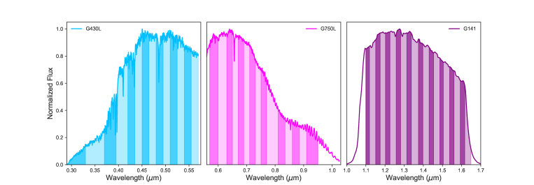
Figure 1: Example stellar spectra for the HST STIS G430L (blue; left), STIS G750L (pink; middle), and WFC3 G141 (purple; right) grisms. Vertical bands indicate the wavelength bins adopted for the spectrophotometric light curves (§3.2).

We reduced the STIS G430L and G750L spectra using the techniques described in Nikolov et al. 2014, 2015 and Alam et al. 2018, which we summarize briefly here. We used the CALSTIS pipeline (version 3.4) to bias-, dark-, and flat-field correct the raw 2D data frames. To identify and correct for cosmic ray events, we used median-combined difference images to flag bad pixels and interpolate over them. We then extracted 1D spectra from the calibrated .flt files and extracted light curves using aperture widths of 6 to 18 pixels, with a step size of 1. Based on the lowest photometric dispersion in the out-of-transit baseline flux, we selected an aperture of 13 pixels for use in our analysis. We computed the mid-exposure time in MJD for each exposure. From the x1d files, we re-sampled all of the extracted spectra and cross-correlated them to a common rest frame to obtain a wavelength solution. Since the cross-correlation measures the shift of each stellar spectrum with respect to the first spectrum of the time series, we re-sampled the spectra to align them and remove sub-pixel drifts associated with the different locations of the spacecraft on its orbit (Huitson et al., 2013). Example spectra for the G430L and G750L gratings are shown in Figure 1.

2.2 HST/WFC3

We observed a single transit of HAT-P-32Ab with the Wide Field Camera 3 (WFC3) instrument on UT 2016 January 21. The transit observation consisted of five consecutive HST orbits, with 18 spectra taken during each orbit. At the beginning of the first orbit, we took an image of the target using the F139M filter with an exposure time of 29.664 seconds. We then obtained time series spectroscopy with the G141 grism (1.1$-$1.7 $\mu$m). Following standard procedure for WFC3 observations of bright targets (e.g., Deming et al. 2013; Kreidberg et al. 2014; Evans et al. 2016; Wakeford et al. 2017), we used the spatial scan observing mode to slew the telescope in the spatial direction during an exposure. This technique allows for longer exposures without saturating the detector (McCullough & MacKenty, 2012). We read out using the SPARS10 sampling sequence with five non-destructive reads per exposure (NSAMP=5), which resulted in integration times of 89 seconds.

We started our analysis of the WFC3 spectra using the flat-fielded and bias-subtracted ima files produced by the CALWF3 pipeline (version 3.3). We extracted the flux for each exposure by taking the difference between successive reads and then subtracting the median flux in a box 32 pixels away from the stellar spectrum. This background subtraction technique masks the area surrounding the 2D spectrum to suppress contamination from nearby stars and companions, including the M dwarf companion to HAT-P-32A. We then corrected for cosmic ray events using the method of Nikolov et al. (2014).

Stellar spectra were extracted by summing the flux within a rectangular aperture centered on the scanned spectrum along the full dispersion axis and along the cross-dispersion direction ranging from 48 to 88 pixels. We determined the wavelength solution by cross-correlating each stellar spectrum to a grid of simulated spectra from the WFC3 Exposure Time Calculator (ETC) with temperatures ranging from 4060$-$9230 K. The closest matching model spectrum to HAT-P-32A ($T_{eff}$ = 6000 K) was the 5860 K model. We used this process to determine shifts along the dispersion axis over the course of the observations.

2.3 Spitzer/IRAC

We obtained two transit observations of HAT-P-32Ab on UT 2012 November 18 and UT 2013 March 19 with the Spitzer Infrared Array Camera (IRAC) 3.6 $\mu$m and 4.5 $\mu$m channels, respectively (Werner et al. 2004; Fazio et al. 2004). Each IRAC exposure was taken over integration times of 2 seconds in the 32 x 32 pixel subarray mode. We reduced the 3.6 and 4.5 $\mu$m Spitzer/IRAC data using a custom data analysis pipeline which implements pixel-level decorrelation (PLD; Deming et al. 2015), described fully in Baxter et al. (in prep). In summary, the pipeline performs a full search of the data reduction parameter space in order to determine the optimum aperture photometry, background subtraction, and centroiding. The resulting photometric light curve is normalized to the out-of-transit flux, and errors are scaled with the photon noise. We clipped outliers with a sliding 4$\sigma$ median filter.

2.4 Photometric Activity Monitoring

Table 1: Summary of photometric observations for HAT-P-32Ab

Season	$N_{obs}$	Date Range	Sigma
		(HJD - 2,450,000)	(mag)
2014-15	79	56943–57114	0.00269
2015-16	82	57293–57472	0.00280
2016-17	55	57706–57843	0.00270
2017-18	13	58172–58288	0.00264
2018-19	41	58384–58510	0.00249

Stellar activity can mimic planetary signals and imprint spectral slopes and spurious absorption features in transmission spectra (e.g., Pont et al. 2013; McCullough et al. 2014). To assess whether stellar activity might impact the transit observations, we inspected available ground-based photometry from the All-Sky Automated Survey for Supernovae (ASAS-SN) (Shappee et al. 2014; Kochanek et al. 2017; Rackham et al. 2017) and the Tennessee State University (TSU) Celestron 14-inch (C14) automated imaging telescope (AIT) at Fairborn Observatory. Since the ASAS-SN data set exhibits large scatter ($\sigma$ $\sim$ 10 mmag) and is dominated by noise, we only use the AIT observations in our analysis of the host star’s activity levels.

We acquired a total of 270 nightly observations of HAT-P-32A over the past five observing seasons from 2014-15 to 2018-19 (see e.g., Henry 1999; Eaton et al. 2003). The first three observing seasons were discussed in Nikolov et al. (2018a), where we provide details about the observing and data reduction procedures. On the basis of those three observing seasons, we concluded that HAT-P-32A is constant on night-to-night timescales within the precision ($\sim$2 mmag) of our observations and likely to be constant on year-to-year timescales.

The SBIG STL-1001E CCD camera on the AIT suffered a failure early in the 2017-18 observing season and had to be replaced, resulting in an abbreviated fourth observing season. The camera was replaced with another SBIG STL-1001E CCD to minimize instrumental shifts in the long-term data. Nonetheless, we found that the 2017-18 and 2018-19 observing seasons had seasonal mean differential magnitudes several milli-magnitudes different from the earlier data. The observations are summarized in Table 1, but we have not included measurements of the seasonal mean magnitudes because of the calibration uncertainties. We note that the small nightly scatter in the new data is consistent with the star remaining constant within the precision of our data on night-to-night timescales.

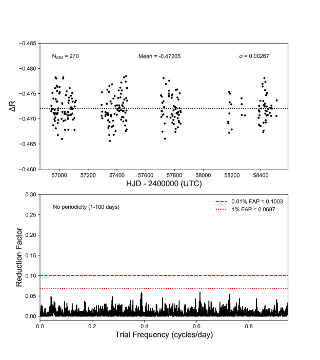
Figure 2: Top: Photometry of HAT-P-32A across five observing seasons from 2014-15 to 2018-19, acquired in the Cousins R band with the TSU Celestron-14 AIT at Fairborn Observatory. The observations have been normalized so that all observing seasons have the same mean as the first season. Bottom: Periodogram of the normalized 2014-2019 observations showing the lack of any significant periodicity between 1 and 100 days. We are therefore unable to detect any rotational variability in our observations.

The complete HAT-P-32A AIT data set is plotted in the top panel of Figure 2, where the data have been normalized so that each seasonal-mean differential magnitude is the same as the first observing season. The bottom panel shows a Lomb-Scargle periodogram (Lomb 1976; Scargle 1982) of our complete data set, which shows no evidence for any coherent periodicity between 1 and 100 days.

We further consider XMM-Newton observations taken on UT 2019 August 30 (P.I.: Sanz-Forcada). These observations reveal an X-ray flux of $L_{\rm X}=2\times 10^{29}$ erg s^-1 in the EPIC cameras using $d=291.5$ pc (Gaia DR2), in addition to the presence of two small flares (see further details in Sanz-Forcada et al., in prep.). EPIC cannot separate the A and B components of the HAT-P-32 system; so although the emission most likely comes from the A component, part of it might originate from the M dwarf companion. Considering this possibility, we checked observations from the optical monitor (OM) onboard XMM-Newton with the UVW2 filter ($\lambda=1870-2370~{}\AA$). These observations indicate a low-level of activity in HAT-P-32A while the companion is not detected, reinforcing the idea that most of the X-ray emission originates from the A component of the system. The UV and X-ray observations, which are most sensitive to the star’s chromosphere, reveal some level of activity, while HAT-P-32A’s photosphere (probed by the optical ground-based monitoring) appears quiet. Given these discrepant results, we decided to fit for activity in our retrievals as described in more detail in §4.3.

3 HST & Spitzer Light Curve Fits

We extracted the 0.3$-$0.5 $\mu$m transmission spectrum of HAT-P-32Ab following the methods of Sing et al. 2011, 2013, Nikolov et al. 2014, and Alam et al. 2018. For each light curve, we simultaneously fit for the transit and systematic effects by fitting a two-component function consisting of a transit model multiplied by a systematics detrending model. The fitting procedure for the STIS, WFC3, and IRAC white light curves is described in §3.1. The fitting procedure for the HST spectroscopic light curves is detailed in §3.2.

3.1 White Light Curves

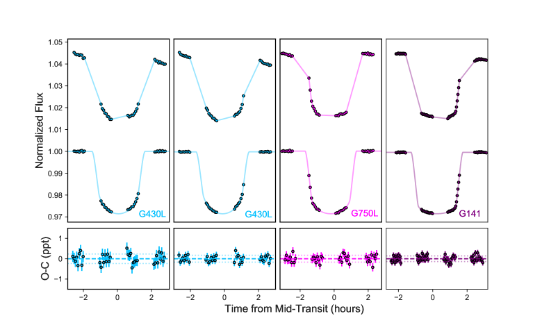
Figure 3: Top: The raw and detrended white light curves (excluding the first orbit and the first exposure of each subsequent orbit) for each HST visit in the STIS G430L (blue), STIS G750L (pink), and WFC3 G141 (purple) grisms. The best-fit analytical light curve model is overplotted. Bottom: Transit fit residuals (in parts per thousand) with error bars.

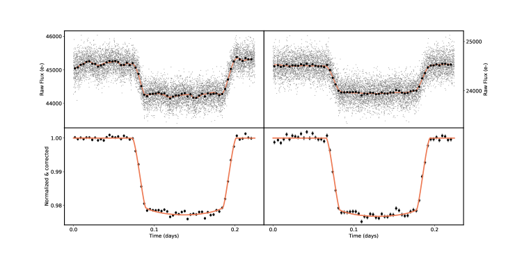
Figure 4: Top: Raw flux (gray points) for the 3.6 $\mu$m (left) and 4.5 $\mu$m (right) Spitzer/IRAC transit light curves, overlaid with the light curve binned to five minutes (black points). Bottom: Detrended light curves (black points) with the best-fit transit model (red line) overplotted.

We produced the white light curves for the HST and Spitzer data sets by summing the flux of the stellar spectra across the full spectrum. We fit the white light curves using a complete analytic transit model (Mandel & Agol, 2002) parametrized by the mid-transit time $T_{0}$, orbital period $P$, inclination $i$, normalized planet semi-major axis $a/R_{\star}$, and planet-to-star radius ratio $R_{p}/R_{\star}$ (see §3.1.1 and §3.1.2 below). The raw and detrended white light curves are shown in Figures 3 and 4. The derived system parameters for HAT-P-32Ab from these fits are given in Table 2.

Table 2: White light curve derived system parameters for HAT-P-32Ab

	STIS G430L (visit 72)	STIS G430L (visit 73)	STIS 750L (visit 74)	WFC3 G141	Spitzer/IRAC
Period, $P$ [days]	2.15 (fixed)	2.15 (fixed)	2.15 (fixed)	2.15 (fixed)	2.15 (fixed)
Orbital inclination, $i$ [∘]	89.53 $\pm$ 1.02	88.97 $\pm$ 0.20	88.50 $\pm$ 1.02	87.78 $\pm$ 0.5	89.55 $\pm$ 0.5
Orbital eccentricity, $e$	0.0 (fixed)	0.0 (fixed)	0.0 (fixed)	0.0 (fixed)	0.0 (fixed)
Scaled semi-major axis, $a/R_{\star}$	5.98 $\pm$ 0.05	5.96 $\pm$ 0.06	6.22 $\pm$ 0.11	6.17 $\pm$ 0.03	6.13 $\pm$ 0.04
Radius ratio, $R_{p}/R_{\star}$	0.1516 $\pm$ 0.0002	0.1510 $\pm$ 0.0002	0.1499 $\pm$ 0.0003	0.1511 $\pm$ 0.0002	0.1502 $\pm$ 0.0009

3.1.1 STIS

To produce the STIS white light curves, we summed each spectrum over the complete bandpasses (2892$-$5700 Å  for the G430L grating; 5240$-$10270 Å  for the G750L grating) and derived photometric uncertainties based on pure photon statistics. The raw white light curves exhibited typical STIS systematic trends related to the spacecraft’s orbital motion (Gilliland et al. 1999; Brown 2001). We detrended these instrumental systematics by applying orbit-to-orbit flux corrections that account for the spacecraft orbital phase ($\phi_{t}$), drift of the spectra on the detector ($x$ and $y$), the shift of the stellar spectrum cross-correlated with the first spectrum of the time series ($\omega$), and time ($t$). Following common practice, we excluded the first orbit and the first exposure of each subsequent orbit because these data were taken while the telescope was thermally relaxing into its new pointing position and have unique, complex systematics (Huitson et al., 2013).

We then generated a family of systematics models spanning all possible combinations of detrending variables and performed separate fits including each systematics model in the two-component function. We assumed zero eccentricity, fixed $P$ to the value given in Hartman et al. (2011), and fit for $i$, $a/R_{\star}$, $T_{0}$, $R_{p}/R_{\star}$, instrument systematic trends, and stellar baseline flux. We derived the four non-linear stellar limb darkening coefficients based on 3D stellar models (Magic et al., 2015) and adopted these values as fixed parameters in the transit fits. We used a Levenberg-Marquardt least-squares fitting routine (Markwardt, 2009) to determine the best-fit parameters of the combined transit+systematics function. We marginalized over the entire set of functions following the Gibson (2014) framework, and selected which systematics model to use based on the lowest Akaike Information Criterion (AIC; Akaike 1974) value (Nikolov et al., 2014). See Appendix A for further details.

3.1.2 WFC3

To produce the WFC3 white light curve, we integrated the flux in each spectrum over the full G141 grism bandpass (1.1$-$1.7 $\mu$m). The raw WFC3 white light curves exhibited typical instrumental systematic trends associated with a visit-long linear slope and the known “ramping” effect in which the flux asymptotically increases over each orbit due to residual charge on the detector from previous exposures (Deming et al. 2013; Huitson et al. 2013; Zhou et al. 2017). In accordance with common practice, the first orbit and the first exposure of each subsequent orbit were excluded due to the well-known charge-trapping ramp systematics for WFC3 (e.g., Kreidberg et al. 2015; Evans et al. 2017).

We then fit the light curve with an analytical model that takes into account the ramping effect and the thermal breathing of HST. We fixed $e$ to zero and $P$ to the value from Hartman et al. 2011, and fit for $i$, $a/R_{\star}$, $R_{p}/R_{\star}$, $T_{0}$, and instrument systematics. We derived the theoretical limb darkening coefficients based on the 3D stellar models of Magic et al. (2015). As in our analysis of the STIS light curves (see §3.1.1), we generated a family of systematics models, detrended the raw WFC3 light curve by performing separate fits to each model, and marginalized over the entire set of functions (c.f. Wakeford et al. 2016 for further details). We used the lowest AIC value to select which model to use. For further details on the systematics model selection, see Appendix A.

3.1.3 IRAC

We fit the cleaned and normalized IRAC light curves with a batman transit model (Kreidberg, 2015) in combination with the PLD systematic model and temporal ramp, resulting in 14 free parameters (four batman, nine PLD, and one temporal ramp). Furthermore, we fixed the eccentricity $e$ to zero and the orbital period $P$ to the literature value of 2.15 days (Hartman et al., 2011), and fit for $i$, $a/R_{\star}$, $T_{0}$, and $R_{p}/R_{star}$. We used the linear limb darkening law to calculate the theoretical limb darkening coefficients using the 1D ATLAS code presented in Sing (2010). Posteriors for all 14 free parameters were calculated using the Markov Chain Monte Carlo (MCMC) script emcee (Foreman-Mackey et al., 2013). The final transit parameters presented in Table 2 are the result of a second MCMC, where the semi-major axis $a/R_{\star}$ and the inclination $i$ were varied within Gaussian priors from the median and standard deviation of the initial fits.

From these fits, we derive $R_{p}/R_{\star}$ values of 0.14663 $\pm$ 0.00034 and 0.14866 $\pm$ 0.00067 for the 3.6 $\mu$m and 4.5 $\mu$m IRAC channels, respectively. Considering the 1.2” x 1.2” pixel size for the Spitzer 32x32 subarray images, we must correct for dilution from the M dwarf companion to HAT-P-32A. We applied the dilution correction derived in Stevenson et al. (2014):

$$\delta_{true}(\lambda)=\delta_{obs}(\lambda)[1+g(\beta,\lambda)\frac{F_{B}}{F_{A}}]$$ (1)

where $\delta_{true}(\lambda)$ is the true (undiluted) transit depth, $\delta_{obs}(\lambda)$ is the observed (diluted) transit depth, $g(\beta,\lambda)$ is wavelength-dependent companion flux fraction inside a photometric aperture of size $\beta$, $F_{B}$ is the flux of the companion star, and $F_{A}$ is the in-transit flux of the primary star. To account for the third light contribution in the Spitzer images, we use the dilution factors of $(F_{B}/F_{A})_{3.6}$ = 0.050$\pm$0.020 and $(F_{B}/F_{A})_{4.5}$ = 0.053$\pm$0.020 from Zhao et al. (2014) and estimate $g(\beta,\lambda)$ for an aperture radius of 2.5 pixels using the IRAC point response function (PRF) at 1/5th pixel sampling. The resulting $R_{p}/R_{\star}$ values corrected for dilution are reported in Tables 2 and 3.

3.2 Spectroscopic Light Curves

Table 3: Broadband HST+Spitzer transmission spectrum for HAT-P-32Ab & adopted non-linear (HST) and linear (Spitzer) limb darkening coefficients

$\lambda$ (Å)	$R_{p}/R_{*}$	$c_{1}$	$c_{2}$	$c_{3}$	$c_{4}$
2900$-$3300	0.15466 $\pm$ 0.00158	0.3152	0.4420	0.4813	-0.3167
3300$-$3700	0.15281 $\pm$ 0.00088	0.4052	0.6943	-0.2319	0.0273
3700$-$3950	0.15203 $\pm$ 0.00073	0.4069	0.5814	0.0073	-0.1117
3950$-$4200	0.15225 $\pm$ 0.00054	0.3991	0.5794	0.0046	-0.0954
4200$-$4350	0.15084 $\pm$ 0.00093	0.4025	0.5039	0.0782	-0.1137
4350$-$4500	0.15104 $\pm$ 0.00068	0.4998	0.3418	0.1836	-0.1546
4500$-$4650	0.15126 $\pm$ 0.00066	0.5702	0.2601	0.0992	-0.0640
4650$-$4800	0.15104 $\pm$ 0.00063	0.5660	0.3170	-0.0081	-0.0204
4800$-$4950	0.15083 $\pm$ 0.00065	0.6888	0.1103	0.1042	-0.0767
4950$-$5100	0.15093 $\pm$ 0.00049	0.6243	0.1792	0.0510	-0.0290
5100$-$5250	0.15137 $\pm$ 0.00059	0.6077	0.1870	0.0812	-0.0633
5250$-$5400	0.15183 $\pm$ 0.00049	0.6782	0.0034	0.2548	-0.1367
5400$-$5550	0.15080 $\pm$ 0.00051	0.7363	-0.0980	0.2614	-0.1063
5550$-$5700	0.15128 $\pm$ 0.00060	0.7356	-0.1217	0.2683	-0.1016
5700$-$6000	0.15077 $\pm$ 0.00070	0.7728	-0.2053	0.3104	-0.1130
6000$-$6300	0.15105 $\pm$ 0.00058	0.7964	-0.2947	0.3789	-0.1381
6300$-$6500	0.15057 $\pm$ 0.00122	0.8037	-0.3285	0.4036	-0.1533
6500$-$6700	0.14924 $\pm$ 0.00075	0.8718	-0.4706	0.4820	-0.1819
6700$-$6900	0.14933 $\pm$ 0.00072	0.8333	-0.4336	0.4641	-0.1631
6900$-$7100	0.15066 $\pm$ 0.00069	0.8462	-0.4889	0.5201	-0.1886
7100$-$7300	0.15121 $\pm$ 0.00097	0.8461	-0.4985	0.5090	-0.1780
7300$-$7500	0.15022 $\pm$ 0.00058	0.8321	-0.4776	0.4849	-0.1740
7500$-$7700	0.15084 $\pm$ 0.00071	0.8520	-0.5558	0.5665	-0.2086
7700$-$8100	0.14905 $\pm$ 0.00073	0.8573	-0.5815	0.5666	-0.2010
8100$-$8350	0.15021 $\pm$ 0.00110	0.8645	-0.6135	0.5794	-0.2024
8350$-$8600	0.15080 $\pm$ 0.00122	0.8574	-0.6348	0.6070	-0.2167
8600$-$8850	0.15013 $\pm$ 0.00110	0.8560	-0.6383	0.5907	-0.2071
8850$-$9100	0.15105 $\pm$ 0.00189	0.8622	-0.6681	0.6155	-0.2188
9100$-$9500	0.14906 $\pm$ 0.00146	0.8598	-0.6768	0.6389	-0.2305
9500$-$10200	0.14939 $\pm$ 0.00113	0.8479	-0.6659	0.6118	-0.2182
11190$-$11470	0.15071 $\pm$ 0.00035	0.6341	-0.2157	0.1764	-0.0625
11470$-$11750	0.15068 $\pm$ 0.00031	0.6336	-0.2103	0.1587	-0.0553
11750$-$12020	0.15136 $\pm$ 0.00033	0.6311	-0.2011	0.1333	-0.0413
12020$-$12300	0.15119 $\pm$ 0.00030	0.6282	-0.1673	0.0809	-0.0204
12300$-$12580	0.15055 $\pm$ 0.00028	0.6318	-0.1698	0.0748	-0.0191
12580$-$12860	0.15065 $\pm$ 0.00032	0.6566	-0.1844	0.0366	-0.0005
12860$-$13140	0.15048 $\pm$ 0.00035	0.6480	-0.1651	0.0284	0.0051
13140$-$13420	0.15148 $\pm$ 0.00027	0.6588	-0.1768	0.0249	0.0089
13420$-$13700	0.15204 $\pm$ 0.00033	0.6724	-0.1969	0.0252	0.0125
13700$-$13980	0.15168 $\pm$ 0.00030	0.6987	-0.2291	0.0299	0.0157
13980$-$14260	0.15182 $\pm$ 0.00030	0.7189	-0.2589	0.0426	0.0140
14260$-$14540	0.15202 $\pm$ 0.00029	0.7400	-0.3024	0.0668	0.0091
14540$-$14820	0.15122 $\pm$ 0.00039	0.7750	-0.3619	0.1059	-0.0025
14820$-$15090	0.15180 $\pm$ 0.00034	0.8033	-0.4316	0.1561	-0.0152
15090$-$15370	0.15067 $\pm$ 0.00036	0.8629	-0.5486	0.2411	-0.0365
15370$-$15650	0.15172 $\pm$ 0.00039	0.8773	-0.6057	0.3004	-0.0586
15650$-$15930	0.15114 $\pm$ 0.00036	0.8491	-0.5982	0.3194	-0.0704
15930$-$16210	0.15015 $\pm$ 0.00039	0.9445	-0.8091	0.5039	-0.1343
16210$-$16490	0.14947 $\pm$ 0.00042	0.9501	-0.8296	0.5057	-0.1253
36000	0.14820 $\pm$ 0.00078	0.1816 $\pm$ 0.0048	–	–	–
45000	0.15020 $\pm$ 0.00087	0.1614 $\pm$ 0.0051	–	–	–

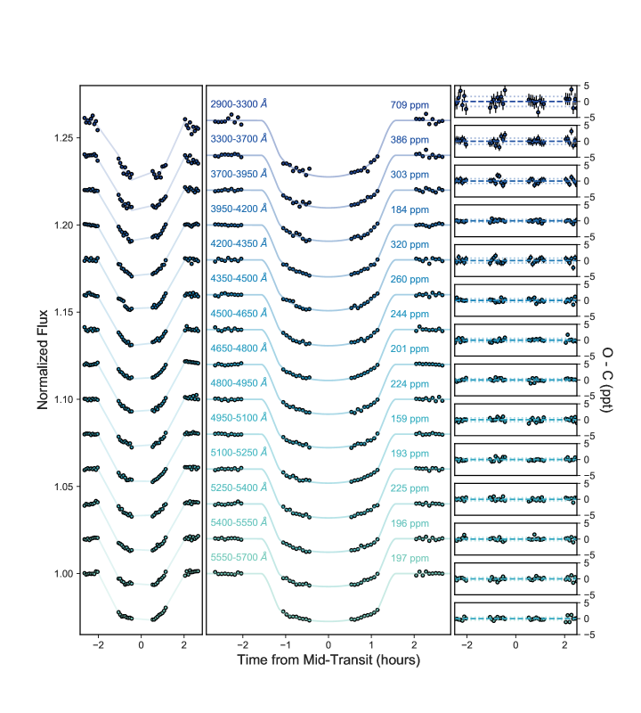
Figure 5: HST/STIS G430L (visit 72) spectrophotometric light curves. The common mode corrected raw (left) and detrended (middle) light curves shown for each wavelength bin are offset vertically by an arbitrary constant for clarity. The observed minus computed residuals (parts per thousand) with error bars are shown in the right panel.

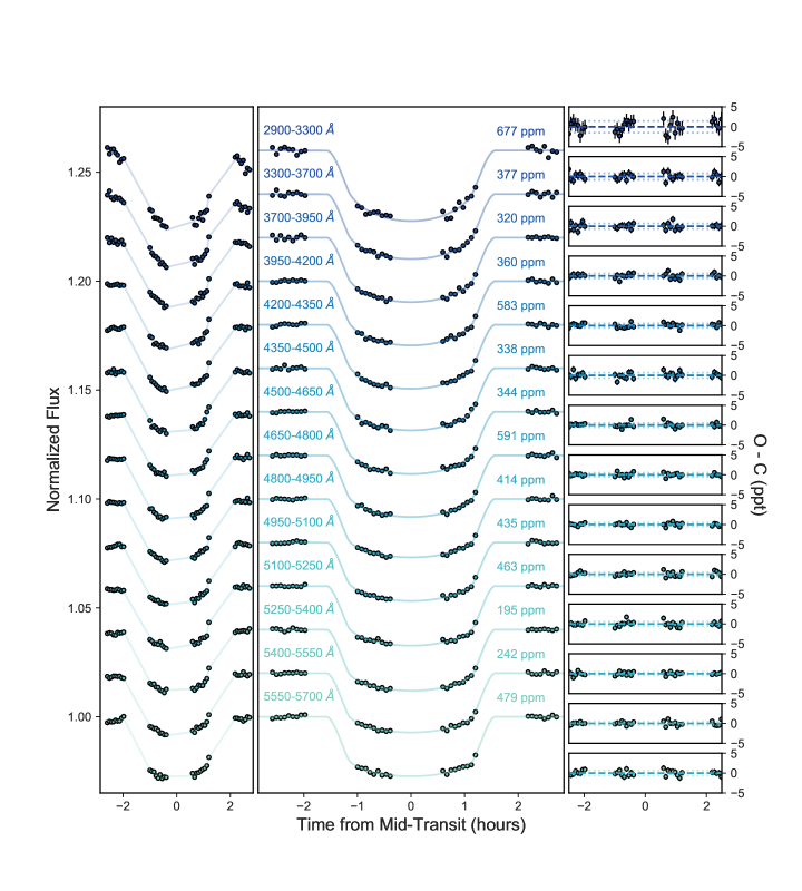
Figure 6: Same as Figure 5, but for HST/STIS G430L visit 73.

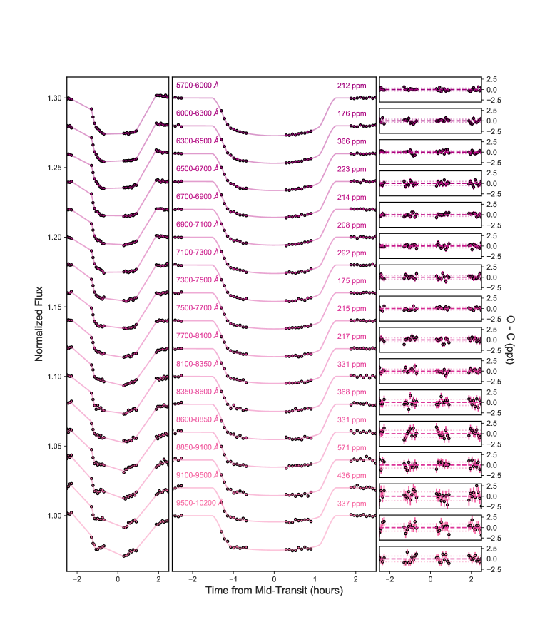
Figure 7: Same as Figure 5, but for HST/STIS G750L visit 74.

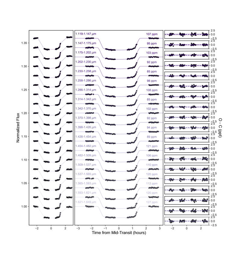
Figure 8: Same as Figure 5, but for HST/WFC3 G141 visit 01.

To produce the spectroscopic light curves, we binned the STIS and WFC3 spectra into 49 spectrophotometric channels between 0.3$-$1.7 $\mu$m. The resulting binned light curves are shown in Figures 5, 6, 7, and 8. We produced 30 STIS spectrophotometric light curves by summing the flux of the stellar spectra in bins with widths ranging from 0.015 to 0.04 $\mu$m. We used a range of bin widths to achieve similar fluxes in each spectroscopic channel as well as avoid stellar absorption lines. To generate the 19 WFC3 spectroscopic light curves, we summed the flux of the stellar spectra in uniformly sized bins of six pixels (0.028 $\mu$m) each.

We performed a common mode correction to remove wavelength-independent systematic trends from each spectroscopic channel and reduce the amplitude of the observed HST breathing systematics. Common mode trends are computed by dividing the raw flux of the white light curve in each grating by the best-fitting transit model. We applied the common mode correction by dividing each spectrophotometric light curve by the computed common mode flux, which may cause offsets between the independent data sets. We then fit each spectroscopic light curve following the same procedure as the white light curves (see §3.1.1 and §3.1.2 for details), but fixed $T_{0}$ to the white light curve best-fit value. We also fixed $i$ and $a/R_{\star}$ to the values from Hartman et al. (2011) to reduce the effect of instrumental offsets between the different datasets. The limb darkening coefficients were fixed to the computed theoretical values for each wavelength bin (see Table 3). The measured $R_{p}/R_{\star}$ values for each spectroscopic channel are presented in Table 3.

4 Results

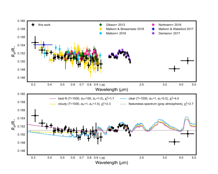
Figure 9: Top: Broadband transmission spectrum for HAT-P-32Ab from HST STIS+WFC3 and Spitzer IRAC (black points). Ground-based measurements from Gibson et al. 2013 (green), Mallonn & Strassmeier 2016 (yellow), Mallonn et al. 2016 (light blue), Nortmann et al. 2016 (pink), Mallonn & Wakeford 2017 (dark blue), and Damiano et al. 2017 (purple) are shown for comparison. Bottom: A subset of the best-fitting theoretical models (lines) fit to the broadband transmission spectrum. The increase in transit depth near 1.4 $\mu$m corresponds to a near-infrared H₂O bandhead. The average $R_{p}/R_{\star}$ baseline of the transmission spectrum (dashed black line) is shown for reference.

We construct the optical to infrared transmission spectrum for HAT-P-32Ab measured from 0.3$-$5 $\mu$m by combining the STIS, WFC3, and Spitzer observations. The broadband spectrum (Table 3) compared to previous atmospheric observations and forward models (Goyal et al. 2018, 2019) is presented in Figure 9. In this section, we characterize the shape and slope of the transmission spectrum compared to previous atmospheric observations (§4.1) and present an interpretation of the planet’s atmospheric structure and composition based on fits to a grid of 1D radiative-convective equilibrium models (§4.2) and retrievals (§4.3).

4.1 HST+Spitzer Transmission Spectrum & Comparison with Previous Results

The optical to infrared transmission spectrum of HAT-P-32Ab is characterized by a weak H₂O absorption feature at 1.4 $\mu$m, no evidence of Na i or K i alkali absorption features, and a steep slope in the blue optical. This continuum slope may be due to the presence of an optical opacity source in the atmosphere of this planet, which Mallonn & Wakeford (2017) predict could be magnesium silicate aerosols. Additionally, we note that the reddest spectroscopic channels of the WFC3 observations ($\sim$1.57$-$1.65 $\mu$m) present a steep slope in the H₂O bandhead at $\sim$1.6 $\mu$m. This feature is also present in the independently reduced WFC3 results of Damiano et al. (2017), suggesting that it may be physical in nature and not an artifact of the data reduction process. This feature is not well modeled by the best-fitting ATMO models (§4.2) or PLATON retrievals (§4.3) and we note that it has been observed for other planets, such as the HAT-P-26b (Wakeford et al., 2017) and WASP-79b (Sotzen et al., 2020).

There are several other measured transmission spectra for HAT-P-32Ab in addition to the HST spectrum reported here, including observations from Gemini/GMOS (Gibson et al., 2013), LBT/MODS (Mallonn et al., 2016), GTC/OSIRIS (Nortmann et al., 2016), and LBC/LBT (Mallonn & Wakeford, 2017). Figure 9 shows our results compared to previously published optical and near-infrared transmission spectra. Cloud-free atmospheric models predict Na i at 5893 Å and K i at 7665 Å, but ground-based optical transmission spectra of HAT-P-32Ab show no evidence of these pressure-broadened absorption features in addition to a Rayleigh-scattering slope (Gibson et al. 2013; Mallonn et al. 2016; Mallonn & Strassmeier 2016; Nortmann et al. 2016; Tregloan-Reed et al. 2018). We varied the size of the spectroscopic channels centered on Na i and K i to search for absorption signatures from these species and confirm no evidence of these features in the spectrum at the precision level of our data.

Our STIS, WFC3, and Spitzer measurements are consistent with these previous ground-based observations in terms of the slope and shape of the transmission spectrum, as well as the $R_{p}/R_{\star}$ baseline. Small offsets among data sets can be attributed to systematic errors, different data reduction techniques, and the challenges of measuring absolute transit depths from observations taken during different epochs as the stellar photosphere evolves (e.g., Stevenson et al. 2014; Kreidberg et al. 2015). The agreement in the HAT-P-32Ab absolute transit depth measurements over several epochs, using ground-based as well as space-borne facilities, and with different instruments susceptible to different systematic effects reiterates the lack of variability in the photosphere of the stellar host (§2.4).

4.2 Fits to Forward Atmospheric Models

We compare our observed HST+Spitzer transmission spectrum (Figure 9) to the publicly available generic grid of forward model transmission spectra presented in Goyal et al. 2018, 2019. The 1D radiative-convective equilibrium models are produced using ATMO (Amundsen et al. 2014; Tremblin et al. 2015, 2016; Drummond et al. 2016), computed assuming isothermal pressure-temperature ($P-T$) profiles and condensation without rainout (local condensation). The models include opacities due to H₂-H₂, H₂-He collision induced absorption, H₂O, CO₂, CO, CH₄, NH₃, Na, K, Li, Rb, Cs, TiO, VO, FeH, CrH, PH₃, HCN, C₂H₂, H₂S, and SO₂. The pressure broadening sources for these species are tabulated in Goyal et al. (2018).

The entire generic ATMO grid comprises 56,320 forward model transmission spectra for 22 equilibrium temperatures (400$-$2600 K in steps of 100 K), four planetary gravities (5, 10, 20, 50 m/s²), five metallicities (1, 10, 50, 100, 200 x solar), and four C/O ratios (0.35, 0.56, 0.7, 1.0), as well as varying degrees of haziness (1, 10, 150, 1100) and cloudiness (0.0, 0.06, 0.20, 1.0). Gray scattering clouds are included in the models using the H₂ cross-section at 350 nm as a reference wavelength; the varying degrees of cloudiness are a multiplicative factor to this value.

We fit the generic ATMO model grid scaled to $g$ = 5 m/s² to the observed spectrum by computing the mean model prediction for the wavelength range of each spectroscopic channel (see Table 3) and performing a least-squares fit of the band-averaged model to the spectrum. In the fitting procedure, we preserved the shape of the model by allowing the vertical offset in $R_{p}/R_{\star}$ between the spectrum and model to vary while holding all other parameters fixed. The number of degrees of freedom for each model is $n-m$, where $n$ is the number of data points and $m$ is the number of fitted parameters. Since $n$ = 51 and $m$ = 1, the number of degrees of freedom for each model is constant. From the fits, we quantified our model selection by computing the $\chi^{2}$ statistic.

The best-fitting model is shown in the bottom panel of Figure 9, which also shows a flat model, and representative cloudy and clear atmosphere models for reference. The best fitting model ($\chi_{r}^{2}$ = 1.7) corresponds to a cloudy ($\alpha_{cloud}$ = 1.0) and slightly hazy ($\alpha_{haze}$ = 150) atmosphere, with a temperature of $T$ = 1000 K, super-solar metallicity ([Fe/H] = +1.7), and sub-solar C/O (C/O = 0.35). The selected clear ($\chi_{r}^{2}$ = 4.5) and cloudy models ($\chi_{r}^{2}$ = 2.3) are similar to the best fitting model, but with no clouds or hazes ($\alpha_{haze}$ = 0.0, $\alpha_{cloud}$ = 0.0) and extreme cloudiness ($\alpha_{cloud}$ = 1.0), respectively. The flat model ($\chi_{r}^{2}$ = 2.7) represents a gray (featureless) spectrum. The models shown here do not predict that Na i or K i should be present in the transmission spectrum, indicating that these species may be depleted in the atmosphere of HAT-P-32Ab (Burrows & Sharp, 1999).

4.3 Retrieving HAT-P-32Ab’s Atmospheric Properties

Table 4: PLATON atmospheric retrieval results for HAT-P-32Ab

Parameter	HST+Spitzer
Planetary radius, $R_{p}$ [$R_{J}$]	1.96${}_{-0.00}^{+0.00}$
Isothermal temperature, T [K]	1248${}_{-92}^{+92}$
Metallicity, log(Z)	2.41${}_{-0.07}^{+0.06}$
Carbon-to-oxygen ratio, C/O	0.12${}_{-0.04}^{+0.08}$
Cloudtop pressure, log($P_{cloud}$ [Pa])	3.61${}_{-1.03}^{+0.91}$
Scattering, log(scattering factor)	1.00${}_{-0.28}^{+0.37}$
Scattering slope	9.02${}_{-1.00}^{+0.58}$

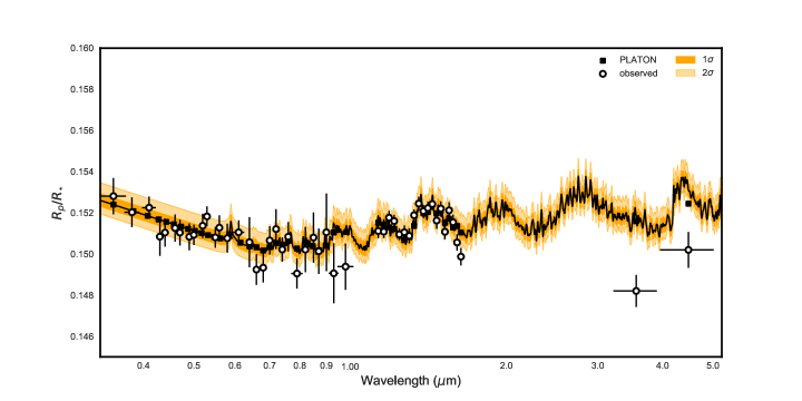
Figure 10: Transmission spectrum of HAT-P-32Ab measured with HST+Spitzer (open circles). The best-fit model binned to the resolution of the data (squares) and the median fit to the retrieved spectrum (black line) are shown. The shaded regions indicate the 1$\sigma$ (medium orange) and 2$\sigma$ (light orange) credible intervals.

Although the forward model fits described in §4.2 well match the red optical and near-infrared portions of the transmission spectrum, the best-fitting model poorly constrains the data in the blue optical. We therefore retrieve the atmospheric properties of our HST+Spitzer transmission spectrum using the Python-based PLanetary Atmospheric Transmission for Observer Noobs (PLATON) (Zhang et al., 2019) code to better constrain HAT-P-32Ab’s atmosphere. The results of the full optical to infrared retrieval analysis for this planet are shown in Figure 10 and Table 4.

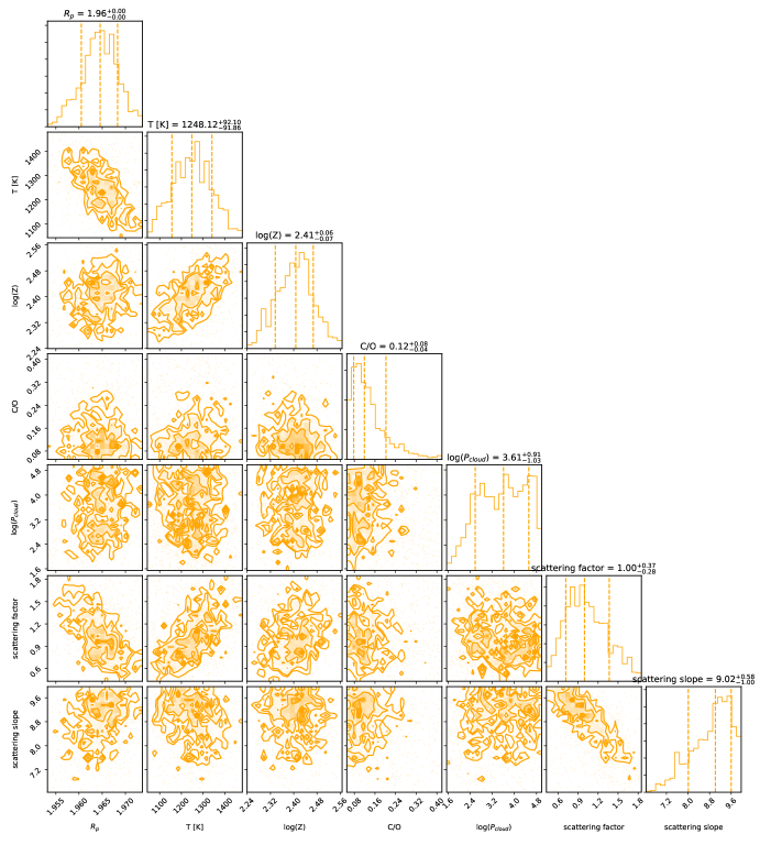
Figure 11: Pairs plot showing distributions of retrieved parameters from the HST+Spitzer transmission spectrum. We show constraints on the planetary radius, temperature of the isothermal planet atmosphere, metallicity (in solar units), C/O, cloud-top pressure (in Pascals), log(scattering factor), and scattering slope.

We constrain the planetary radius $R_{p}$, temperature of the isothermal part of the atmosphere $T_{p}$, atmospheric metallicity log($Z$), carbon-to-oxygen ratio C/O, cloud-top pressure $P_{cloud}$, the factor by which the absorption coefficient is stronger than Rayleigh scattering at the reference wavelength of 1 $\mu$m (log(scattering factor)), and the scattering slope. We use flat priors for $R_{p}$, $T_{p}$, log($Z$), and C/O, with upper and lower bounds for $R_{p}$ and $T_{p}$ from Tregloan-Reed et al. (2018). Our metallicity and C/O priors are set by PLATON’s pre-computed equilibrium chemistry grid (Zhang et al., 2019). Pairs plots showing the distributions of retrieved parameters. are presented in Figure 11. We initially performed our retrievals including activity in our fits (parametrized by spot size and temperature contrast), but found that the model with no stellar heterogeneities was preferred. This finding is consistent with the star appearing quiet in the optical photometry as described in §2.4. We therefore adopt the results from the fits without activity henceforth in the paper.

The results of our retrieval fits to the HST+Spitzer spectrum are summarized in Table 4. The best-fit retrieved spectrum is consistent with an isothermal temperature of 1248${}_{-92}^{+92}$ K, a thick cloud deck, enhanced Rayleigh scattering, and $\sim$10x H₂O abundance. The inferred atmospheric metallicity of 2.41${}_{-0.07}^{+0.06}$ x solar follows the observed mass-metallicity trend for the Solar System. We also retrieve a sub-solar C/O of 0.12${}_{-0.04}^{+0.08}$, a log cloudtop pressure of 3.61${}_{-1.03}^{+0.91}$, a scattering factor of 1.00${}_{-0.28}^{+0.37}$, and a scattering slope of 9.02${}_{-1.00}^{+0.58}$.

In comparison with the best-fitting ATMO forward model (§4.2), we note that the estimated subsolar values for C/O from our ATMO and PLATON fits confirm the presence of clouds in the atmosphere of this planet (Helling et al., 2019). The atmospheric metallicity from ATMO (log($Z$) $\sim$ -0.04; Bertelli et al. 1994), however, does not well match the constrained PLATON metallicity for the broadband HST+Spitzer spectrum.

The retrieved limb temperature from PLATON is lower than the equilibrium temperature of HAT-P-32Ab. This finding is in accordance with other retrieval results from the literature in which retrieved temperatures have been found to be notably cooler ($\sim$200$-$600 K) than planetary equilibrium temperatures (c.f. Table 1 of MacDonald et al. 2020). These lower retrieved temperatures appear to be the result of applying 1D atmospheric models to planetary spectra with different morning-evening terminator compositions (MacDonald et al., 2020). Although 1D retrievals provide an acceptable fit to observations, they artificially shift atmospheric parameters away from terminator-averaged properties. As a result, the retrieved temperature profiles are hundreds of degrees cooler and have weaker temperature gradients than reality.

Furthermore, our retrieval and forward model fits confirm a cloudy atmosphere for this planet. Our findings also corroborate previous PanCET results for this planet suggesting a Bond albedo of $A_{B}$ $<$ 0.4 and poor atmospheric re-circulation (Nikolov et al., 2018a), consistent with the measured geometric albedo of $A_{g}$ $<$ 0.2 for this planet by Mallonn et al. (2019), as well as previous studies showing that planets with higher stellar irradiation levels have greater day-night temperature contrasts and lower re-circulation efficiencies (e.g., Schwartz, & Cowan 2015; Kataria et al. 2016; Schwartz et al. 2017).

5 HAT-P-32Ab in Context

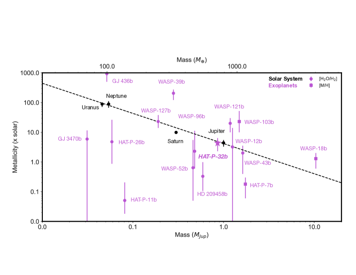
Figure 12: The observed mass-metallicity trend for transiting exoplanets with metallicity constraints from [H₂O/H₂] (purple points) or [M/H] (purple squares) and the Solar System gas and ice giants (black points). The dashed black line corresponds to a linear fit in log-log space to the Solar System points.

We interpret the optical to infrared transmission spectrum of HAT-P-32Ab in light of the observed mass-metallicity relation for exoplanets and theoretical predictions for inferring a priori the presence of clouds in exoplanet atmospheres. Our retrieval of the 0.3$-$5.0 $\mu$m HST+Spitzer spectrum is consistent with the presence of a thick cloud deck, enhanced Rayleigh scattering, and $\sim$10x solar H₂O abundance. This value is consistent with the H₂O abundance constraint for HAT-P-32Ab’s atmosphere inferred by Damiano et al. (2017) using an independent reduction of the WFC3 data set only. Based on the metallicity inferred from PLATON (log($Z/Z_{\odot}$) = 2.41${}_{-0.07}^{+0.06}$), we find that HAT-P-32Ab follows the expected mass-metallicity trend for exoplanets based on our Solar System gas giants (e.g., Kreidberg et al. 2014; Wakeford et al. 2018). Figure 12 shows HAT-P-32Ab among other exoplanets with metallicity constraints from water abundances (or a sodium abundance constraint in the case of WASP-96b; Nikolov et al. 2018b), compared to the Solar System gas and ice giants.

Furthermore, the fractional change in atmospheric scale height (H₂O$-$J) has been suggested as a near-infrared diagnostic for the degree of cloudiness of an exoplanet atmosphere (Stevenson, 2016). We measure the strength of the water feature using the method of Stevenson (2016), which requires computing the difference in transit depth between the J-band peak (1.36$-$1.44 $\mu$m) and baseline (1.22$-$1.30 $\mu$m) spectral regions and then dividing by the change in transit depth $\Delta D$, which corresponds to a one scale height change in altitude. $\Delta D$ is given by the relation $\Delta D$ $\sim$ 2$HR_{p}$/$R_{\star}^{2}$, where $H$ is the atmospheric scale height, $R_{p}$ is the planetary radius, and $R_{\star}$ is the stellar radius. $H$ is computed using an equilibrium temperature assuming the planet has zero albedo (i.e., absorbs all incident flux) and consequently re-radiates that energy over its entire surface as a blackbody of that temperature. With a sample of 12, the Stevenson (2016) study found that planets with equilibrium temperatures higher than 700 K and surface gravities greater than log($g$) = 2.8 (cgs) are more likely to be cloud-free (Stevenson, 2016).

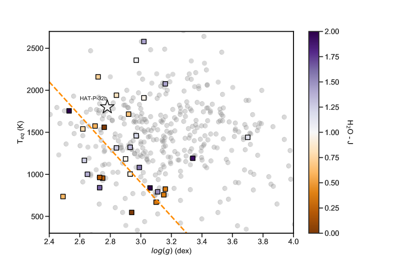
Figure 13: Amplitude of the observed 1.4 $\mu$m H₂O bandhead as a function of planetary equilibrium temperature and surface gravity (squares), color coded by the strength of the feature. Exoplanets with mass and radius measurements (gray circles) are shown for reference. The dashed orange line shows the proposed divide (Stevenson, 2016) to delineate between cloudy versus clear planets in the $T_{eq}$ $-$ log($g$) phase space. HAT-P-32Ab (white star) crosses this proposed divide and falls in the region theorized to be populated by clear atmosphere planets.

We similarly search for trends in cloudiness in the $T_{eq}$ $-$ log($g$) phase space using the expanded sample of 37 planets for which we can measure the H₂O$-$J index, shown in Figure 13. We use the WFC3 data presented in Wakeford et al. (2019), reduced in a uniformly consistent manner, to compute H₂O$-$J. We note that the reductions from Tsiaras et al. (2018) also present consistent results. We find that several planets lie along the proposed divide (Stevenson, 2016) to delineate between two classes of cloudy versus clear planets in the $T_{eq}$ $-$ log($g$) phase space. For our more complete sample, the trend is further muddled by the fact that planets such as HAT-P-32Ab with flat transmission spectra indicating the presence of clouds, fall in the region of this parameter space theorized to be populated by cloud-free planets. Moreover, the optical cloudiness index set forth by Heng (2016) suggests that more irradiated planets are more likely to be cloud-free. With a planetary temperature constraint of $T_{p}$ = 1801 $\pm$ 18 K (Tregloan-Reed et al., 2018), HAT-P-32Ab does not fit this prediction as it is a highly irradiated planet with a thick cloud layer. These findings suggest that other physical parameters impact cloud opacities in the atmospheres of close-in giant exoplanets and therefore need to be considered in interpreting atmospheric observations.

6 Summary

We measured the transmission spectrum of the hot Jupiter HAT-P-32Ab over the 0.3$-$5 $\mu$m wavelength range with HST+Spitzer transit observations. Below we summarize our conclusions about the atmospheric properties of this planet based on these measurements.

• The transmission spectrum is characterized by an optical Rayleigh scattering slope, a weak H₂O feature at 1.4 $\mu$m, and no evidence of alkali absorption features. Compared to a grid of 1D radiative-convective equilibrium models, the best-fitting model indicates the presence of clouds/hazes, consistent with previous ground-based observations (Figure 9).

• We retrieve the planet’s atmospheric properties (Figure 10) using PLATON. The results are consistent with $\sim$10x solar H₂O abundance and are in agreement with the observed mass-metallicity relation for exoplanets (Figure 12).

• We consider theoretical predictions for inferring a priori the presence of clouds in exoplanet atmospheres (Stevenson 2016; Fu et al. 2017). We find that HAT-P-32Ab calls these hypotheses into question, since it is among a handful of planets that cross the proposed divide (Stevenson, 2016) to delineate between two classes of cloudy versus clear exoplanets in the $T_{eq}$ $-$ log($g$) phase space (Figure 13).

Appendix A White Light Curve Systematics Model Selection

As described in §3.1.1 and §3.1.2, we detrended the HST white light curves using a family of systematics models spanning all possible combinations of the detrending parameters for STIS and WFC3 (c.f. Appendix B1 of Alam et al. 2018 for further details). For each of the systematics models used, we performed separate fits for each model and marginalized over the entire set of models, assuming equally weighted priors. Table A1 lists the combinations of detrending parameters for the STIS and WFC3 systematics models. For both data sets, the model with the lowest Aikake Information Criterion (AIC) value was selected for detrending. The selection of these models is summarized in Table A2.

Table A1: HST white light curve systematics models

	Model
STIS G430L models
1	$\phi_{t}+\phi^{2}_{t}+\phi^{3}_{t}+\phi^{4}_{t}+t$
2	$\phi_{t}+\phi^{2}_{t}+\phi^{3}_{t}+\phi^{4}_{t}+t+\omega+x^{2}$
3	$\phi_{t}+\phi^{2}_{t}+\phi^{3}_{t}+\phi^{4}_{t}+t+x+y^{2}$
4	$\phi_{t}+\phi^{2}_{t}+\phi^{3}_{t}+\phi^{4}_{t}+t+x^{2}+y$
5	$\phi_{t}+\phi^{2}_{t}+\phi^{3}_{t}+\phi^{4}_{t}+t+\omega$
6	$\phi_{t}+\phi^{2}_{t}+\phi^{3}_{t}+\phi^{4}_{t}+t+x$
7	$\phi_{t}+\phi^{2}_{t}+\phi^{3}_{t}+\phi^{4}_{t}+t+\omega+x^{2}+y$
8	$\phi_{t}+\phi^{2}_{t}+\phi^{3}_{t}+\phi^{4}_{t}+t+x+x^{2}+y$
9	$\phi_{t}+\phi^{2}_{t}+\phi^{3}_{t}+\phi^{4}_{t}+t+y$
10	$\phi_{t}+\phi^{2}_{t}+\phi^{3}_{t}+\phi^{4}_{t}+t+\omega+x$
11	$\phi_{t}+\phi^{2}_{t}+\phi^{3}_{t}+\phi^{4}_{t}+t+\omega+y$
12	$\phi_{t}+\phi^{2}_{t}+\phi^{3}_{t}+\phi^{4}_{t}+t+\omega+x+y$
13	$\phi_{t}+\phi^{2}_{t}+\phi^{3}_{t}+\phi^{4}_{t}+t+\omega+\omega^{2}+y$
14	$\phi_{t}+\phi^{2}_{t}+\phi^{3}_{t}+\phi^{4}_{t}+t+\omega+x+x^{2}$
15	$\phi_{t}+\phi^{2}_{t}+\phi^{3}_{t}+\phi^{4}_{t}+t+\omega+y+y^{2}$
16	$\phi_{t}+\phi^{2}_{t}+\phi^{3}_{t}+\phi^{4}_{t}+t+x+y$
17	$\phi_{t}+\phi^{2}_{t}+\phi^{3}_{t}+\phi^{4}_{t}+t+\omega+\omega^{2}+x$
18	$\phi_{t}+\phi^{2}_{t}+\phi^{3}_{t}+\phi^{4}_{t}+t+x+x^{2}$
19	$\phi_{t}+\phi^{2}_{t}+\phi^{3}_{t}+\phi^{4}_{t}+t+x+x^{2}+y$
20	$\phi_{t}+\phi^{2}_{t}+\phi^{3}_{t}+\phi^{4}_{t}+t+y+y^{2}$
21	$\phi_{t}+\phi^{2}_{t}+\phi^{3}_{t}+\phi^{4}_{t}+t+y$
22	$\phi_{t}+\phi^{2}_{t}+\phi^{3}_{t}+\phi^{4}_{t}+t+\omega+\omega^{2}+x$
23	$\phi_{t}+\phi^{2}_{t}+\phi^{3}_{t}+\phi^{4}_{t}+t+\omega+\omega^{2}+x+y$
24	$\phi_{t}+\phi^{2}_{t}+\phi^{3}_{t}+\phi^{4}_{t}+t+\omega+\omega^{2}+x+x^{2}+y+y^{2}$
25	$\phi_{t}+\phi^{2}_{t}+\phi^{3}_{t}+\phi^{4}_{t}+t+\omega+\omega^{2}+x+x^{2}+y^{2}$
STIS G750L models
1	$\phi_{t}+\phi^{2}_{t}+\phi^{3}_{t}+\phi^{4}_{t}+t$
2	$\phi_{t}+\phi^{2}_{t}+\phi^{3}_{t}+\phi^{4}_{t}+t+\omega+x$
3	$\phi_{t}+\phi^{2}_{t}+\phi^{3}_{t}+\phi^{4}_{t}+t+x+y^{2}$
4	$\phi_{t}+\phi^{2}_{t}+\phi^{3}_{t}+\phi^{4}_{t}+t+\omega^{2}$
5	$\phi_{t}+\phi^{2}_{t}+\phi^{3}_{t}+\phi^{4}_{t}+t+\omega$
6	$\phi_{t}+\phi^{2}_{t}+\phi^{3}_{t}+\phi^{4}_{t}+t+x$
7	$\phi_{t}+\phi^{2}_{t}+\phi^{3}_{t}+\phi^{4}_{t}+t+\omega+x^{2}+y^{3}$
8	$\phi_{t}+\phi^{2}_{t}+\phi^{3}_{t}+\phi^{4}_{t}+t+x+y$
9	$\phi_{t}+\phi^{2}_{t}+\phi^{3}_{t}+\phi^{4}_{t}+t+y$
10	$\phi_{t}+\phi^{2}_{t}+\phi^{3}_{t}+\phi^{4}_{t}+t+\omega+x$
11	$\phi_{t}+\phi^{2}_{t}+\phi^{3}_{t}+\phi^{4}_{t}+t+\omega+y$
12	$\phi_{t}+\phi^{2}_{t}+\phi^{3}_{t}+\phi^{4}_{t}+t+\omega+x+y$
13	$\phi_{t}+\phi^{2}_{t}+\phi^{3}_{t}+\phi^{4}_{t}+t+y$
14	$\phi_{t}+\phi^{2}_{t}+\phi^{3}_{t}+\phi^{4}_{t}+t+\omega+x^{2}$
15	$\phi_{t}+\phi^{2}_{t}+\phi^{3}_{t}+\phi^{4}_{t}+t+\omega+y+y^{2}$
16	$\phi_{t}+\phi^{2}_{t}+\phi^{3}_{t}+\phi^{4}_{t}+t+\omega+y+y^{2}+y^{3}$
17	$\phi_{t}+\phi^{2}_{t}+\phi^{3}_{t}+\phi^{4}_{t}+t+\omega+\omega^{2}+x$
18	$\phi_{t}+\phi^{2}_{t}+\phi^{3}_{t}+\phi^{4}_{t}+t+x+y^{2}$
19	$\phi_{t}+\phi^{2}_{t}+\phi^{3}_{t}+\phi^{4}_{t}+t+x$
20	$\phi_{t}+\phi^{2}_{t}+\phi^{3}_{t}+\phi^{4}_{t}+t+y+y^{2}$
21	$\phi_{t}+\phi^{2}_{t}+\phi^{3}_{t}+\phi^{4}_{t}+t+y+y^{2}+y^{3}$
22	$\phi_{t}+\phi^{2}_{t}+\phi^{3}_{t}+\phi^{4}_{t}+t+\omega+\omega^{2}+x$
23	$\phi_{t}+\phi^{2}_{t}+\phi^{3}_{t}+\phi^{4}_{t}+t+\omega+\omega^{2}+x+y$
24	$\phi_{t}+\phi^{2}_{t}+\phi^{3}_{t}+\phi^{4}_{t}+t+\omega+\omega^{2}+x+y$
25	$\phi_{t}+\phi^{2}_{t}+\phi^{3}_{t}+\phi^{4}_{t}+t+\omega+\omega^{2}+x^{2}$
WFC3 G141 models
1	$a_{hst2}+a_{hst3}+a_{hst4}+a_{x1}+a_{x2}+a_{x3}+a_{y1}+a_{y2}+a_{y3}+a_{t1}$
2	$a_{hst3}+a_{hst4}+a_{x1}+a_{x2}+a_{x3}+a_{y1}+a_{y2}+a_{y3}+a_{t1}$
3	$a_{hst4}+a_{x1}+a_{x2}+a_{x3}+a_{y1}+a_{y2}+a_{y3}+a_{t1}$
4	$a_{x1}+a_{x2}+a_{x3}+a_{y1}+a_{y2}+a_{y3}+a_{t1}$
5	$a_{hst3}+a_{x1}+a_{x2}+a_{x3}+a_{y1}+a_{y2}+a_{y3}+a_{t1}$
6	$a_{hst2}+a_{hst4}+a_{x1}+a_{x2}+a_{x3}+a_{y1}+a_{y2}+a_{y3}+a_{t1}$
7	$a_{hst2}+a_{x1}+a_{x2}+a_{x3}+a_{y1}+a_{y2}+a_{y3}+a_{t1}$
8	$a_{hst2}+a_{hst3}+a_{x1}+a_{x2}+a_{x3}+a_{y1}+a_{y2}+a_{y3}+a_{t1}$
9	$a_{hst3}+a_{hst4}+a_{x1}+a_{x2}+a_{x3}+a_{y1}+a_{y2}+a_{y3}+a_{t1}$
10	$a_{hst4}+a_{x1}+a_{x2}+a_{x3}+a_{y1}+a_{y2}+a_{y3}+a_{t1}$
11	$a_{x1}+a_{x2}+a_{x3}+a_{y1}+a_{y2}+a_{y3}+a_{t1}$
12	$a_{hst3}+a_{x1}+a_{x2}+a_{x3}+a_{y1}+a_{y2}+a_{y3}+a_{t1}$
13	$a_{hst2}+a_{hst4}+a_{x1}+a_{x2}+a_{x3}+a_{y1}+a_{y2}+a_{y3}+a_{t1}$
14	$a_{hst2}+a_{x1}+a_{x2}+a_{x3}+a_{y1}+a_{y2}+a_{y3}+a_{t1}$

Table A2: Systematics model selection for the STIS & WFC3 white light curves

Model	$\chi_{r}^{2}$	AIC	d.o.f
STIS G430L (visit 72)
1	1.75	65.07	28
2	1.60	61.63	26
3	1.62	62.21	26
4	1.76	65.76	26
5	1.54	59.68	27
6	1.57	60.41	27
7	1.73	64.78	27
8	1.41	57.24	25
9	1.58	61.01	26
10	1.55	60.84	25
11	1.60	61.63	26
12	1.40	57.00	25
13	1.63	62.87	25
14	1.58	61.95	24
15	1.63	62.82	25
16	1.55	61.16	24
17	1.44	58.66	24
18	1.62	62.21	26
19	1.67	62.83	25
20	1.78	66.24	26
21	1.53	60.30	25
22	1.55	60.65	25
23	1.59	62.27	24
24	1.70	65.39	22
25	1.56	63.24	20
STIS G430L (visit 73)
1	2.76	90.53	27
2	2.75	88.77	25
3	1.79	64.84	25
4	2.08	52.03	25
5	2.78	90.77	26
6	2.43	81.39	26
7	2.06	71.57	26
8	2.52	82.54	24
9	2.13	73.24	25
10	2.11	72.54	24
11	2.88	91.95	25
12	2.99	93.95	24
13	2.11	72.63	24
14	2.60	83.85	23
15	1.65	61.59	24
16	1.72	63.46	23
17	2.56	82.81	23
18	2.49	82.24	25
19	2.57	83.61	24
20	1.58	59.59	25
21	1.64	61.46	24
22	2.52	82.50	24
23	2.13	73.02	23
24	1.70	63.63	21
25	1.79	66.00	19
STIS G750L (visit 74)
1	1.99	57.10	27
2	1.74	50.82	25
3	2.06	59.96	25
4	1.62	53.93	25
5	2.03	53.82	26
6	1.99	59.03	26
7	1.73	56.01	26
8	1.99	55.67	25
9	1.76	53.18	25
10	1.76	54.84	24
11	1.97	55.68	25
12	2.03	53.82	26
13	1.69	54.83	24
14	1.72	46.94	23
15	1.83	54.71	24
16	1.89	56.18	23
17	2.03	57.10	24
18	1.79	53.42	25
19	1.70	47.31	24
20	1.80	57.61	25
21	1.85	59.32	24
22	2.03	57.10	24
23	1.82	56.59	23
24	1.83	51.60	21
25	1.67	61.00	21
WFC3 G141 visit 01
1	1.08	80.20	52
2	1.07	78.62	53
3	2.10	133.51	54
4	2.94	179.86	55
5	1.44	97.54	54
6	1.99	127.59	53
7	2.39	149.55	54
8	1.14	82.38	53
9	1.04	78.09	52
10	1.08	79.32	53
11	1.66	109.82	54
12	1.46	99.28	53
13	1.07	79.41	52
14	1.23	87.09	53

References

- Akaike (1974) Akaike, H. 1974, IEEE Transactions on Automatic Control, 19, 716.
- Alam et al. (2018) Alam, M. K., Nikolov, N., López-Morales, M., et al. 2018, AJ, 156, 298 2018, AJ, 156, 298.
- Amundsen et al. (2014) Amundsen, D. S., Baraffe, I., Tremblin, P., et al. 2014, A&A, 564, A59.
- Arcangeli et al. (2018) Arcangeli, J., Désert, J.-M., Line, M. R., et al. 2018, ApJ, 855, L30.
- Benneke et al. (2019) Benneke, B., Knutson, H. A., Lothringer, J., et al. 2019, Nature Astronomy, 3, 813.
- Bertelli et al. (1994) Bertelli, G., Bressan, A., Chiosi, C., et al. 1994, A&AS, 106, 275
- Brown (2001) Brown, T. M. 2001, ApJ, 553, 1006.
- Burrows & Sharp (1999) Burrows, A., & Sharp, C. M. 1999, ApJ, 512, 843.
- Carter & Winn (2009) Carter, J. A., & Winn, J. N. 2009, ApJ, 704, 51.
- Chachan et al. (2019) Chachan, Y., Knutson, H. A., Gao, P., et al. 2019, AJ, 158, 244.
- Charbonneau et al. (2002) Charbonneau, D., Brown, T. M., Noyes, R. W., & Gilliland, R. L. 2002, ApJ, 568, 377.
- Charbonneau et al. (2005) Charbonneau, D., Allen, L. E., Megeath, S. T., et al. 2005, ApJ, 626, 523.
- Charbonneau et al. (2008) Charbonneau, D., Knutson, H. A., Barman, T., et al. 2008, ApJ, 686, 1341.
- Chen et al. (2017) Chen, G., Pallé, E., Nortmann, L., et al. 2017, A&A, 600, L11.
- Ciardi et al. (2015) Ciardi, D. R., Beichman, C. A., Horch, E. P., et al. 2015, ApJ, 805, 16.
- Claret (2000) Claret, A. 2000, A&A, 363, 1081.
- Crossfield (2015) Crossfield, I. J. M. 2015, PASP, 127, 941.
- Damiano et al. (2017) Damiano, M., Morello, G., Tsiaras, A., et al. 2017, AJ, 154, 39.
- Deming et al. (2013) Deming, D., Wilkins, A., McCullough, P., et al. 2013, ApJ, 774, 95.
- Deming et al. (2015) Deming, D., Knutson, H., Kammer, J., et al. 2015, ApJ, 805, 132
- Deming & Seager (2017) Deming, L. D., & Seager, S. 2017, Journal of Geophysical Research (Planets), 122, 53.
- Deming et al. (2019) Deming, D., Louie, D., & Sheets, H. 2019, PASP, 131, 013001.
- Drummond et al. (2016) Drummond, B., Tremblin, P., Baraffe, I., et al. 2016, A&A, 594, A69.
- Eaton et al. (2003) Eaton, J. A., Henry, G. W., & Fekel, F. C. 2003, Astrophysics and Space Science Library, 288, 189.
- Espinoza et al. (2019) Espinoza, N., Rackham, B. V., Jordán, A., et al. 2019, MNRAS, 482, 2065.
- Evans et al. (2016) Evans, T. M., Sing, D. K., Wakeford, H. R., et al. 2016, ApJ, 822, L4.
- Evans et al. (2017) Evans, T. M., Sing, D. K., Kataria, T., et al. 2017, Nature, 548, 58.
- Evans et al. (2018) Evans, T. M., Sing, D. K., Goyal, J. M., et al. 2018, AJ, 156, 283.
- Fazio et al. (2004) Fazio, G. G., Hora, J. L., Allen, L. E., et al. 2004, The Astrophysical Journal Supplement Series, 154, 10.
- Foreman-Mackey et al. (2013) Foreman-Mackey, D., Hogg, D. W., Lang, D., et al. 2013, PASP, 125, 306
- Fu et al. (2017) Fu, G., Deming, D., Knutson, H., et al. 2017, ApJ, 847, L22.
- Garland & Irwin (2019) Garland, R., & Irwin, P. G. J. 2019, arXiv e-prints, arXiv:1903.03997.
- Gibson et al. (2013) Gibson, N. P., Aigrain, S., Barstow, J. K., et al. 2013, MNRAS, 436, 2974.
- Gibson (2014) Gibson, N. P. 2014, MNRAS, 445, 3401.
- Gilliland et al. (1999) Gilliland, R. L., Goudfrooij, P., & Kimble, R. A. 1999, Publications of the Astronomical Society of the Pacific, 111, 1009.
- Goyal et al. (2018) Goyal, J. M., Mayne, N., Sing, D. K., et al. 2018, MNRAS, 474, 5158.
- Goyal et al. (2019) Goyal, J. M., Mayne, N., Sing, D. K., et al. 2019, MNRAS, 486, 783
- Hartman et al. (2011) Hartman, J. D., Bakos, G. Á., Torres, G., et al. 2011, ApJ, 742, 59.
- Helling (2018) Helling, C. 2018, arXiv:1812.03793.
- Helling et al. (2019) Helling, C., Iro, N., Corrales, L., et al. 2019, A&A, 631, A79
- Heng (2016) Heng, K. 2016, ApJ, 826, L16.
- Henry (1999) Henry, G. W. 1999, PASP, 111, 845.
- Huitson et al. (2013) Huitson, C. M., Sing, D. K., Pont, F., et al. 2013, MNRAS, 434, 3252.
- Huitson et al. (2017) Huitson, C. M., Désert, J.-M., Bean, J. L., et al. 2017, AJ, 154, 95.
- Irwin et al. (2008) Irwin, P. G. J., Teanby, N. A., de Kok, R., et al. 2008, J. Quant. Spec. Radiat. Transf., 109, 1136
- Jordán et al. (2013) Jordán, A., Espinoza, N., Rabus, M., et al. 2013, ApJ, 778, 184.
- Kataria et al. (2016) Kataria, T., Sing, D. K., Lewis, N. K., et al. 2016, ApJ, 821, 9
- Kirk et al. (2019) Kirk, J., López-Morales, M., Wheatley, P. J., et al. 2019, AJ, 158, 144
- Knutson et al. (2008) Knutson, H. A., Charbonneau, D., Allen, L. E., et al. 2008, ApJ, 673, 526.
- Kochanek et al. (2017) Kochanek, C. S., Shappee, B. J., Stanek, K. Z., et al. 2017, Publications of the Astronomical Society of the Pacific, 129, 104502.
- Kreidberg et al. (2014) Kreidberg, L., Bean, J. L., Désert, J.-M., et al. 2014, Nature, 505, 69.
- Kreidberg (2015) Kreidberg, L. 2015, PASP, 127, 1161
- Kreidberg et al. (2015) Kreidberg, L., Line, M. R., Bean, J. L., et al. 2015, ApJ, 814, 66
- Kreidberg (2017) Kreidberg, L. 2017, Handbook of Exoplanets, Edited by Hans J. Deeg and Juan Antonio Belmonte. Springer Living Reference Work, ISBN: 978-3-319-30648-3, 2017, id.100, 100
- Knutson et al. (2012) Knutson, H. A., Lewis, N., Fortney, J. J., et al. 2012, ApJ, 754, 22.
- Knutson et al. (2014) Knutson, H. A., Dragomir, D., Kreidberg, L., et al. 2014, ApJ, 794, 155.
- Kurucz (1993) Kurucz, R. L. 1993, VizieR Online Data Catalog , VI/39.
- Lecavelier Des Etangs et al. (2008) Lecavelier Des Etangs, A., Vidal-Madjar, A., Désert, J.-M., & Sing, D. 2008, A&A, 485, 865.
- Lewis et al. (2013) Lewis, N. K., Knutson, H. A., Showman, A. P., et al. 2013, ApJ, 766, 95.
- Lomb (1976) Lomb, N. R. 1976, Ap&SS, 39, 447
- Louden et al. (2017) Louden, T., Wheatley, P. J., Irwin, P. G. J., Kirk, J., & Skillen, I. 2017, MNRAS, 470, 742.
- MacDonald et al. (2020) MacDonald, R. J., Goyal, J. M., & Lewis, N. K. 2020, arXiv e-prints, arXiv:2003.11548.
- Magic et al. (2015) Magic, Z., Chiavassa, A., Collet, R., et al. 2015, A&A, 573, A90.
- Mallonn et al. (2016) Mallonn, M., Bernt, I., Herrero, E., et al. 2016, MNRAS, 463, 604.
- Mallonn & Strassmeier (2016) Mallonn, M., & Strassmeier, K. G. 2016, A&A, 590, A100.
- Mallonn & Wakeford (2017) Mallonn, M., & Wakeford, H. R. 2017, Astronomische Nachrichten, 338, 773.
- Mallonn et al. (2019) Mallonn, M., Köhler, J., Alexoudi, X., et al. 2019, A&A, 624, A62.
- Mandel & Agol (2002) Mandel, K., & Agol, E. 2002, ApJ, 580, L171.
- Markwardt (2009) Markwardt, C. B. 2009, Astronomical Data Analysis Software and Systems XVIII, 411, 251.
- Marley et al. (2013) Marley, M. S., Ackerman, A. S., Cuzzi, J. N., et al. 2013, Comparative Climatology of Terrestrial Planets, 367.
- McCullough & MacKenty (2012) McCullough, P., & MacKenty, J. 2012, Space Telescope WFC Instrument Science Report.
- McCullough et al. (2014) McCullough, P. R., Crouzet, N., Deming, D., et al. 2014, ApJ, 791, 55.
- Mighell (2005) Mighell, K. J. 2005, MNRAS, 361, 861.
- Nikolov et al. (2014) Nikolov, N., Sing, D. K., Pont, F., et al. 2014, MNRAS, 437, 46.
- Nikolov et al. (2015) Nikolov, N., Sing, D. K., Burrows, A. S., et al. 2015, MNRAS, 447, 463.
- Nikolov et al. (2018a) Nikolov, N., Sing, D. K., Goyal, J., et al. 2018, MNRAS, 474, 1705.
- Nikolov et al. (2018b) Nikolov, N., Sing, D. K., Fortney, J. J., et al. 2018, Nature, 557, 526.
- Nortmann et al. (2016) Nortmann, L., Pallé, E., Murgas, F., et al. 2016, A&A, 594, A65.
- Pinhas et al. (2019) Pinhas, A., Madhusudhan, N., Gandhi, S., et al. 2019, MNRAS, 482, 1485
- Pont et al. (2013) Pont, F., Sing, D. K., Gibson, N. P., et al. 2013, MNRAS, 432, 2917.
- Rackham et al. (2017) Rackham, B., Espinoza, N., Apai, D., et al. 2017, ApJ, 834, 151.
- Reach et al. (2005) Reach, W. T., Megeath, S. T., Cohen, M., et al. 2005, Publications of the Astronomical Society of the Pacific, 117, 978.
- Scargle (1982) Scargle, J. D. 1982, ApJ, 263, 835
- Schwartz, & Cowan (2015) Schwartz, J. C., & Cowan, N. B. 2015, MNRAS, 449, 4192
- Schwartz et al. (2017) Schwartz, J. C., Kashner, Z., Jovmir, D., et al. 2017, ApJ, 850, 154
- Seager & Sasselov (2000) Seager, S., & Sasselov, D. D. 2000, ApJ, 537, 916.
- Seager & Deming (2010) Seager, S., & Deming, D. 2010, ARA&A, 48, 631.
- Shappee et al. (2014) Shappee, B. J., Prieto, J. L., Grupe, D., et al. 2014, ApJ, 788, 48.
- Sing et al. (2008) Sing, D. K., Vidal-Madjar, A., Désert, J.-M., Lecavelier des Etangs, A., & Ballester, G. 2008, ApJ, 686, 658.
- Sing (2010) Sing, D. K. 2010, A&A, 510, A21.
- Sing et al. (2011) Sing, D. K., Pont, F., Aigrain, S., et al. 2011, MNRAS, 416, 1443
- Sing et al. (2012) Sing, D. K., Huitson, C. M., Lopez-Morales, M., et al. 2012, MNRAS, 426, 1663
- Sing et al. (2013) Sing, D. K., Lecavelier des Etangs, A., Fortney, J. J., et al. 2013, MNRAS, 436, 2956.
- Sing et al. (2015) Sing, D. K., Wakeford, H. R., Showman, A. P., et al. 2015, MNRAS, 446, 2428.
- Sing et al. (2016) Sing, D. K., Fortney, J. J., Nikolov, N., et al. 2016, Nature, 529, 59.
- Sotzen et al. (2020) Sotzen, K. S., Stevenson, K. B., Sing, D. K., et al. 2020, AJ, 159, 5
- Spake et al. (2018) Spake, J. J., Sing, D. K., Evans, T. M., et al. 2018, Nature, 557, 68.
- Stevenson et al. (2014) Stevenson, K. B., Désert, J.-M., Line, M. R., et al. 2014, Science, 346, 838
- Stevenson (2016) Stevenson, K. B. 2016, ApJ, 817, L16.
- Todorov et al. (2013) Todorov, K. O., Deming, D., Knutson, H. A., et al. 2013, ApJ, 770, 102.
- Tremblin et al. (2015) Tremblin, P., Amundsen, D. S., Mourier, P., et al. 2015, ApJ, 804, L17.
- Tremblin et al. (2016) Tremblin, P., Amundsen, D. S., Chabrier, G., et al. 2016, ApJ, 817, L19.
- Tregloan-Reed et al. (2018) Tregloan-Reed, J., Southworth, J., Mancini, L., et al. 2018, MNRAS, 474, 5485.
- Tsiaras et al. (2018) Tsiaras, A., Waldmann, I. P., Zingales, T., et al. 2018, AJ, 155, 156.
- Wakeford et al. (2016) Wakeford, H. R., Sing, D. K., Evans, T., et al. 2016, ApJ, 819, 10
- Wakeford et al. (2017) Wakeford, H. R., Sing, D. K., Kataria, T., et al. 2017, Science, 356, 628.
- Wakeford et al. (2017) Wakeford, H. R., Visscher, C., Lewis, N. K., et al. 2017, MNRAS, 464, 4247
- Wakeford et al. (2018) Wakeford, H. R., Sing, D. K., Deming, D., et al. 2018, AJ, 155, 29.
- Wakeford et al. (2019) Wakeford, H. R., Wilson, T. J., Stevenson, K. B., et al. 2019, Research Notes of the American Astronomical Society, 3, 7.
- Weaver et al. (2020) Weaver, I. C., López-Morales, M., Espinoza, N., et al. 2020, AJ, 159, 13.
- Werner et al. (2004) Werner, M. W., Roellig, T. L., Low, F. J., et al. 2004, The Astrophysical Journal Supplement Series, 154, 1.
- Winn (2010) Winn, J. N. 2010, ArXiv e-prints , arXiv:1001.2010.
- Wyttenbach et al. (2017) Wyttenbach, A., Lovis, C., Ehrenreich, D., et al. 2017, A&A, 602, A36.
- Zhang et al. (2019) Zhang, M., Chachan, Y., Kempton, E. M.-R., & Knutson, H. A. 2019, PASP, 131, 034501.
- Zhao et al. (2014) Zhao, M., O’Rourke, J. G., Wright, J. T., et al. 2014, ApJ, 796, 115.
- Zhou et al. (2017) Zhou, Y., Apai, D., Lew, B. W. P., & Schneider, G. 2017, AJ, 153, 243.