The role of directionality, heterogeneity and correlations in epidemic risk and spread

Abstract

Most models of epidemic spread, including many designed specifically for COVID-19, implicitly assume mass-action contact patterns and undirected contact networks, meaning that the individuals most likely to spread the disease are also the most at risk to receive it from others. Here, we review results from the theory of random directed graphs which show that many important quantities, including the reproduction number and the epidemic size, depend sensitively on the joint distribution of in- and out-degrees (“risk” and “spread”), including their heterogeneity and the correlation between them. By considering joint distributions of various kinds, we elucidate why some types of heterogeneity cause a deviation from the standard Kermack-McKendrick analysis of SIR models, i.e., so-called mass-action models where contacts are homogeneous and random, and some do not. We also show that some structured SIR models informed by realistic complex contact patterns among types of individuals (age or activity) are simply mixtures of Poisson processes and tend not to deviate significantly from the simplest mass-action model. Finally, we point out some possible policy implications of this directed structure, both for contact tracing strategy and for interventions designed to prevent superspreading events. In particular, directed graphs have a forward and backward version of the classic “friendship paradox”—forward edges tend to lead to individuals with high risk, while backward edges lead to individuals with high spread—such that a combination of both forward and backward contact tracing is necessary to find superspreading events and prevent future cascades of infection.

I Introduction

In the field of network epidemiology, populations of hosts are modeled as graphs, where vertices are individuals and edges are contacts along which infectious diseases can spread [1]. Here, we review important concepts from the study of random graphs to inform our understanding of epidemics. We explain how these concepts and results can be used on the one hand to inform interventions and guide policy, and on the other hand to solve common nonlinear models of epidemic spread based on differential equations. Our paper is structured such that the main text focuses on concepts and insights, with all mathematical details presented in complementary boxes and in the Appendix.

To model epidemic spreading with graphs, we consider general transmission graphs where we define edges as contacts or interactions that will transmit the disease from one individual to another should the first individual become infected. These transmission graphs can be generated through a set of assumptions [2, 3], contact tracing data [4], or defined as isomorphic to classic epidemic models [5]. We can then analyze how epidemic outcomes depend on the structure of these transmission graphs [6, 3, 7, 8]. The only assumption we make is that these graphs correspond to non-recurrent epidemic dynamics, i.e., where individuals have a state that represent their immunological status and never go back to previous states. This is true, for example, for infectious diseases that convey lifelong immunity. The Susceptible-Infectious-Recovered (SIR) model is the canonical example of such dynamics, but our discussion also applies to the Susceptible-Exposed-Infectious-Recovered (SEIR) model, or any other non-recurrent compartmental model of disease spread [9]. The fact that individual states are non-recurrent here means that individuals can only be susceptible once and that every contact can only transmit the disease once, which is a key feature that allows us to analyze epidemic models based on the structure of the underlying graph.

Graphs allow us to model many kinds of heterogeneity and structure, and explore how and when heterogeneity affects epidemic thresholds and sizes. For the simplest random graphs, epidemics end up being equivalent to classic mass-action compartmentalized models in epidemiology, which can be analyzed using systems of differential equations. As we will discuss, the SIR model on Erdős-Rényi random graphs, where every pair of vertices is independently connected with the same probability, behaves like the Kermack–McKendrick SIR solution in the limit where the number of vertices—i.e. the population size—is infinitely large [10, 11, 12, 4]. Yet, since the degree of a vertex is the number of edges it has, we can model superspreading events by having a heavy-tailed degree distribution, where some vertices have a degree considerably larger than the mean [13]. A random edge is more likely to be with a high-degree individual, who has more secondary contacts in turn. Thus the average degree of a vertex reached by a random edge is greater than the average degree of a random vertex. This phenomenon is often called the “friendship paradox”: on average, your friends have more friends than you do [14]. In the epidemic context, this phenomenon has two effects. First, the reproduction number is not simply the mean degree; it depends also on its second moment or variance (see Box I). In particular, even if we hold the mean degree constant, increasing the variance lowers the critical transmission rate: the probability of transmission per contact needed to reach the epidemic threshold [2]. Second, as developed in Refs. [15, 16, 17] and recently pointed out as highly relevant for COVID-19 in Refs. [18, 19], the “friendship paradox” can amplify the effectiveness of contact tracing, giving a better chance that a contact leads to a superspreading event, helping the prevention of further cascades of infection.

[b]

This view of superspreading events assumes that the transmission graph is undirected: that is, edges that would spread the disease in one direction would also spread it in the other. While this may be true for individuals who attend a group event or work together in close quarters, some mechanisms of spread, such as surface contacts from handling and delivery, are inherently directed [20]. In graph terms, an individual might have high out-degree but low in-degree, or vice versa. Intuitively, this is because they represent different concepts: in-degree captures the risk that an individual receives the infection from others (network pathways for an incoming transmission event) while out-degree captures the spread that an infected individual can cause once infected (the network pathways for outgoing transmission events). In addition, many non-pharmaceutical interventions to prevent disease spread have a directed effect. Wearing a simple mask is one such mechanism, as it is believed to reduce the probability that the wearer spreads a respiratory disease like COVID-19 to others, but not to strongly protect the wearer from receiving the disease from others [21, 22].

Most importantly, almost all epidemic models—including many mass-action models and models based on undirected contact networks—can be mapped unto epidemic percolation networks (EPNs) [6, 5, 7] which are semi-directed (contain both directed and undirected edges). A directed edge $a\to b$ in an EPN means that $a$ will transmit the disease to $b$ if $a$ becomes infected and $b$ is susceptible, and undirected edges simply correspond to two directed edges in opposite directions. We therefore adopt a general view of directed transmission graphs [20, 23, 8, 6, 24] which allows us to investigate the role of directionality, heterogeneity and correlations in these graphs without the need to specify the complex underlying mechanisms of a spreading dynamics, and without loss of generality.

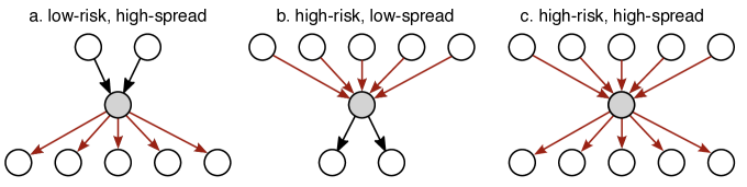
Figure 1: Different types of individuals in a directed graph model of disease spread: a. low-risk, but high-spread, b. high-risk, but low-spread, and c. high-risk and high-spread.

Each vertex in a directed graph has an in-degree, i.e., the number of contacts from whom it could receive the disease, and an out-degree, the number of contacts to whom it could spread the disease if it becomes infected. We can think of the in-degree as the risk of this individual, and the out-degree as their spread. As illustrated in Fig. 1, an individual might contribute to rapid spreading by having high risk, high spread, or both. For instance, an average immunocompromised individual might have high risk but low spread, while someone who fails to wear a mask even while those around them do might have low risk and high spread. Finally, someone who by choice or necessity interacts with many others in close quarters would have both high risk and high spread, as in the traditional undirected picture of superspreading events.

This distinction between risk and spread, or between incoming and outgoing edges, has several consequences. First, the reproduction number is proportional to the correlation between risk and spread (see Box II). More precisely, the contribution of a given vertex to the reproduction number is proportional to the product of its in- and out-degrees. Vertices with both high risk and high spread are likely to become infected and then to infect many others. But if they have either high risk or low spread, then the expectation for the number of new cases they might generate is smaller. This has possible implications for non-pharmaceutical interventions: the effect of reducing an individual’s spread is implicitly proportional to their risk.

[t]

Second, we now have two distinct types of friendship paradox, a forward one and a backward one (see Fig. 2 and Box III). Outgoing edges connect to vertices with probability proportional to their in-degree, so following an edge forward will tend to lead to individuals with high risk. Incoming edges, in contrast, come from vertices with probability proportional to their out-degree, so going following edges backward tends to lead to individuals with high spread.

This suggests that to find superspreading events, and thus to prevent a large number of downstream cases, it may be important to perform backward contract tracing, determining the source of an index case, rather than focusing only on forward contact tracing, finding those who the index case may have infected. As shown in Box III, the average spread of the predecessor of an index case is larger than that of an average successor, especially if the spread has high variance, except in the unusual case where risk and spread are almost perfectly correlated. This insight also implies that the time window we use to define relevant contacts should include their likely predecessor as well as the likely successors of an index case. We can then trace the “siblings” of the index case, i.e., others who were infected by the same individual, and prevent a larger number of future cases.

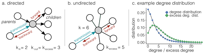
Figure 2: Definitions of key concepts around an index case. (a) In directed graphs, $k_{\mathrm{in}}$ defines the number of potential parents of a vertex and $k_{\mathrm{out}}$ its number of potential children. Backward tracing goes up the genealogical tree toward predecessors while forward tracing goes down the tree toward descendants. Backward tracing will find a biased number of excess outgoing transmissions around the parent (backward friendship paradox, biased spread) while forward tracing would find a biased number of potential parents around the child (forward friendship paradox, biased risk). (b) In undirected graphs, transmissions can go both ways. The identification of parent vertices for backward tracing is therefore only possible after a transmission event. The excess degree of a vertex will then refer to the number of edges other than the one which led to a transmission event and will be equal to the degree minus one (i.e. $k-1$). (c) Example of an undirected degree distribution (blue cross) along with the corresponding excess degree distribution (green diamond). The friendship paradox, i.e. a statistical sampling bias towards higher degree vertices, yields a more skewed tail and higher average in excess degrees than in original degrees.

II Epidemic Probability and Epidemic Size

Here we review some results of Refs. [27, 28] from random graph theory which show how to calculate the epidemic size as a function of the joint distribution of individual risk and spread. We note that these results can be generalized [25, 29] and expanded to include semi-directed graphs composed of a mixture of both directed and undirected edges [26, 20].

As mentioned above, we define the graph such that an edge $a\to b$ means that $a$ will transmit the disease to $b$ if $a$ becomes infected and $b$ is susceptible. These transmission graphs are called epidemic percolation networks (EPNs) [6, 5, 7]. The term “EPN” is often specifically used to refer to transmission graphs whose structure is isomorphic to specific epidemic dynamics and are therefore typically semi-directed. In other words, EPNs consist in randomly chosen subgraphs of a more general graph of contacts that have the potential to transmit the disease, and in which each transmission occurs with some probability. Here we focus on general but purely directed graphs for the sake of simplicity, without affecting the generality of our conclusions (the phenomenology observed below remains the same in the presence of undirected edges). Our approach allows us to consider general forms of heterogeneities and correlations without the need to specify an underlying epidemic dynamics. The connection between general contact networks and EPNs is discussed in Box V.

Let us first compute the epidemic probability, i.e., the probability that a single infected individual generates a large-scale epidemic as opposed to a small outbreak. It helps to think of a process where edges, rather than vertices, propagate the disease from one generation to the next. An outgoing edge produces $j$ “children,” or secondary contacts, if the edge arrives at a vertex with out-degree $j$. A central question in the theory of branching processes is whether the resulting downstream tree of contacts is finite or infinite. Since the total number of descendants of a vertex is finite if and only if this is true of all of its children, the probability of this event obeys a fixed-point equation which can be written compactly using probability generating functions (see Box IV).

Let us now consider the epidemic size. Vertices can receive the infection from one of their incoming edges, or predecessors, who received it from their predecessor in turn. We can thus consider a backwards branching process of incoming edges, where an edge has $i$ “parents” (predecessors upstream in the directed graph) if it comes from a vertex with in-degree $i$. If a vertex has only a finite number of ancestors, counting all upstream vertices, then with high probability none of them will be the index case and it will remain uninfected. But if it has a very large (i.e. infinite) number of ancestors, then with high probability one of its ancestors will be the index case and the vertex will eventually become infected. Thus the calculation of the epidemic size is equivalent to the calculation of the epidemic probability in a time-reversed model, where the disease spreads backward from each vertex to its predecessors.

On undirected graphs, these forward and backward branching processes can often be the same, such that the probability that they die out obeys the same fixed-point equation. This leads to the observation that, in very simple percolation processes, the epidemic size equals the epidemic probability. As explained previously, more complex and realistic processes imply the presence of directed edges, meaning that these two quantities are typically different [2, 26, 20]. Therefore, in the classic SIR dynamics, these fixed-point equations are expected to be different since the EPNs capturing this process are semi-directed (see Box V for details); with the epidemic probability being smaller than the relative size of the epidemic as predicted by the Kermack-McKendrick analysis [5, 30]. In the next section, we consider degree distributions of various kinds and with varying levels of correlation between risk and spread, and look at how these types of heterogeneity affect their epidemic size.

[t]

[t]

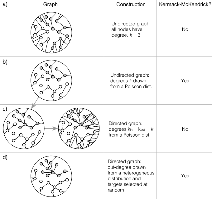
Figure 3: Four examples of transmission graphs, their construction, and whether the Kermack-McKendrick solution corresponds to the expected epidemic size. (a) An undirected graph where all vertices are exactly the same, showing that too much homogeneity is different from mass-action mixing. (b) The simple Poisson graph, the fish out of water, is the only type of undirected transmission graph where the Kermack-McKendrick solution holds. Simple Poisson graphs can be represented with a network structure the expected epidemic size corresponds exactly on that of the classic mass-action models and therefore fail to include important network effects. (c) We take the undirected Poisson graph and add directions to all edges (left). This procedure preserves the in- and out-degree for all vertices. We then rewire the directed edges to obtain a simple graph without overlap between contacts (right). Should we expect the Kermack-McKendrick solution to correctly predict the epidemic size as it did in the original undirected graph? No. (d) A directed graph obtained by independently specifying an in-degree distribution (here Poisson) and an out-degree distribution (here fairly heterogeneous). This corresponds to a situation where all individuals have similar risk of infection, while allowing for superspreading events. Proofs of mapping (or lack thereof) to the Kermack-McKendrick solution are provided in Appendix.

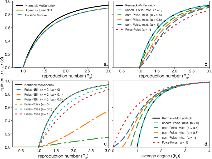
Figure 4: (a) Comparison between Age-structured SIR and Poisson mixture models. The Poisson mixture model presented in Box VI is compared to the numerical integration of the model of Ref. [31] given by Eqs. (23) and to the Kermack-McKendrick solution given by Eq. (18). This comparison showcases the versatility of our approach, and illustrates how many mass-action models similar to Eqs. (23) are equivalent to transmission graphs where in-degrees and out-degrees are a mixture of Poisson distributions when it comes to predicting the epidemic size. (b) Impact of correlations on epidemic size. We consider correlated Poisson mixture model (see Sec. .5 of the Appendix) with $w_{0}=w_{1}=0.5$ and $z_{11}^{\mathrm{in}}=z_{12}^{\mathrm{in}}=z_{21}^{\mathrm{in}}=z_{22}^{\mathrm{in}}$. The parameter $a$ controls the correlation between the in-degrees and out-degrees for vertices of type 1: $a=0$ corresponds to no correlation while $a=1$ corresponds to perfect correlation. The case $a=0$ is equivalent to the uncorrelated scenario explored in Sec. .2 of the Appendix, while the dotted red line corresponds to the fully correlated scenario explored in Sec. .3 of the Appendix. (c) Impact of correlations and heterogeneity on the final epidemic size. In each case study, the in-degree is distributed according to a Poisson [${G_{\mathrm{in}}}(x)=\mathrm{e}^{R_{0}(x-1)}$] and the out-degree is either distributed according to a Poisson [${G_{\mathrm{out}}}(y)=\mathrm{e}^{R_{0}(y-1)}$] or a negative binomial distribution [${G_{\mathrm{out}}}=(1+R_{0}(1-y)/k)^{-k}$]. The parameter $a$ controls the correlation between the in-degrees and out-degrees: $a=0$ corresponds to no correlation while $a=1$ corresponds to perfect correlation, see Eq. (34) for details. The epidemic size, $\mathcal{S}$, and the reproduction number, $R_{0}$, were computed with Eqs. (35c)–(36). The Kermack-McKendrick solution [Eq. (18)] was added to illustrate the impact of heterogeneity and correlations. Importantly, we show that increasing correlations always lead to lower final epidemic size, and that their effect is larger for higher heterogeneity in out-degree. (d) Same results as shown in panel (b) but plotted against the average degree of the populations rather than $R_{0}$. This emphasizes multiple results. First, correlations lower the epidemic threshold. Second, correlations in a subset of the population can lead to sequential epidemic transitions [32, 33], here visible as an S-shaped curve for the cases $a=0.8$ and $a=1.0$. Third, differences between the Kermack-McKendrick and correlated transmission graphs shown in panel (a) are partially hidden in the $R_{0}$ calculation.

III Examples

Let us first consider a simple and random undirected transmission graph, as illustrated in Fig. 3(a-b) whose structure is fully specified by its degree distribution, $P(k)$, setting the number of contacts, $k$, leading to and from a given vertex. Since the graph is undirected, we have $k_{\mathrm{in}}=k_{\mathrm{out}}=k$. One could obtain such a transmission graph by either directly assuming undirected transmission mechanisms such as a percolation process [38] or by starting from epidemic dynamics (e.g., the SIR model) and applying a set of approximations [2]. In the context of EPNs, undirected transmission graphs are possible for simple SI dynamics, or in very specific cases where transmission of a disease is certain over some type of contacts and impossible otherwise. As shown in Ref. [4], the epidemic size $\mathcal{S}$ obtained on these graphs corresponds to the classic Kermack-McKendrick solution, meaning that it is the smallest non-negative solution of

$$\mathcal{S}=1-\mathrm{e}^{-R_{0}\mathcal{S}}\ ,$$ (18)

if and only if the degree distribution is Poisson, i.e., $P(k)=R_{0}^{k}e^{-R_{0}}/k!$ where $R_{0}$ is the reproduction number. What is so special about this distribution? As it turns out, the Poisson distribution is the only one where the excess degree has the same distribution as the degree itself: the probability that an edge leads to $k$ secondary transmissions equals the probability that a random vertex does the same. In terms of the friendship paradox, the probability that you have $k$ friends is the same as the probability that your friend has $k$ friends in addition to you. In particular, these two distributions have the same mean, so $R_{0}=\langle k\rangle$. This is similar to the mass-action hypothesis of Kermack and McKendrick as it implies that information about the contact structure does not matter. For any other degree distribution—even a more homogeneous one as in Fig. 3(a)—the distribution of excess degrees is different from the degree distribution, and the Kermack-McKendrick solution given by Eq. (18) for the epidemic size does not apply.

Consider now a directed version of the Poisson graph. As shown in Fig. 3(c), we can think of undirected edges as bidirectional contacts, i.e. pairs of directed edges, and make this directionality explicit before randomizing the incoming and outgoing edges. What we now have is a graph where in-degrees and out-degrees are equal ($k_{\mathrm{in}}=k_{\mathrm{out}}=k$) and are still drawn from a Poisson distribution, but where incoming and outgoing neighbors are different. Even if the construction of the directed graph structure is very close to that of the undirected case, this directed version does not fall back on the Kermack-McKendrick solution given by Eq. (18) (see Sec. .3 of the Appendix). One key difference can be observed around transmission dead-ends, i.e., vertices with $k_{\mathrm{out}}=0$, which are now impossible to reach since they also have $k_{\mathrm{in}}=0$. In other words, if a vertex has been reached via one if its incoming edges, there is always at least one outgoing edge available to reach the next vertex. As shown in Sec. .2 of the Appendix, equivalence with the Kermack-McKendrick solution is only recovered when in-degrees and out-degrees are uncorrelated.

It turns out that some naive approaches to modeling heterogeneity do not, in fact, alter the epidemic size at all. Consider the following kind of simulation, which would be run until there are no newly infected individuals and where ${P_{\mathrm{out}}}$ is an arbitrary distribution of out-degrees:

1. Start with a single new infectious case in an otherwise susceptible population of size $N$.

2. For each newly infected individual $i$, draw a number $k_{\mathrm{out}}$ of transmissions from the out-degree distribution ${P_{\mathrm{out}}}$.

3. Randomly select $k_{\mathrm{out}}$ individuals from the population. For each one, if it is susceptible then mark it as newly infected and go to step 2, otherwise do nothing.

This type of simulation generates transmission trees similar to the example shown in Fig. 3(d). While the out-degree distribution ${P_{\mathrm{out}}}$ can be arbitrarily heterogeneous, including various kinds of superspreading events, the incoming edges fall with equal probability on every susceptible individual because of the random selection of neighbors at step 3. As a result, the distribution of risk, or in-degree, is Poisson, and the in- and out-degrees are uncorrelated. As shown in Sec. .2 of the Appendix, in the limit of large $N$, the typical epidemic size produced by this kind of simulation exactly corresponds to the Kermack-McKendrick solution regardless of the out-degree distribution ${P_{\mathrm{out}}}$.

These simple examples suggest that the Kermack-McKendrick solution given by Eq. (18) relies on (i) a Poisson distribution of risk among individuals and (ii) a lack of correlation between risk and spread. It does not actually rely on homogeneous spread but only on the independence between the infection risk faced by an individual and the number of secondary infections caused by that individual if infected. The undirected Poisson case, where this independence does not hold since the in- and out-degrees are equal by definition, is somewhat unique since the lack of backtracking and the friendship paradox balance out. We formalize this intuition mathematically in the Appendix, and some important results are visually summarized in Fig. 4.

[t]

IV Connection with structured differential equation models

The mathematical analysis presented thus far is completely general and exact on very large (formally infinite) random directed graphs. To further assess the impact of risk heterogeneity on the epidemic size, we need to look into the mechanisms behind the joint distribution of both risk and spread in specific models. Here we show how one case of these distributions arises from age-structured models in epidemiology.

One particularly powerful and common approach in current models of the COVID-19 pandemic is age-structured SIR or SEIR models (e.g., Refs. [46, 47, 31]) where individuals are separated in different types based on their age and where contacts between age groups are specified through a contact (or “mixing”) matrix. This approach is powerful because it allows the inclusion of important sources of heterogeneity such as different susceptibilities and likelihood of symptoms based on age, and also allows an easy parametrization of interventions such as school closures and/or lockdowns through the contact matrix. Note that the different categories need not be related to age, and could be used to represent other distinguishing properties such as behavior, physiology, employment, etc.

For each group $i$, let us define $S_{i}(t)$, $I_{i}(t)$ and $R_{i}(t)$ as the numbers of Susceptible, Infectious, and Recovered individuals in that group at time $t$. These structured models follow the SIR dynamics through a coupled system of ordinary differential equations written as

$$\dot{S}_{i}(t) =-\beta\sigma_{i}\sum_{j}M_{ij}\frac{I_{j}}{N}S_{i}$$ (23a)

$$\dot{I}_{i}(t) =\beta\sigma_{i}\sum_{j}M_{ij}\frac{I_{j}}{N}S_{i}-\gamma I_{i}$$ (23b)

$$\dot{R}_{i}(t) =\gamma I_{i}$$ (23c)

where $\beta$ is the baseline transmission rate of the disease, $\sigma_{i}$ is the group-dependent susceptibility of individuals, $M_{ij}$ is the average number of contacts someone in group $i$ has with people in group $j$ and through which that individual in group $i$ could become infected, and $\gamma$ is the recovery rate of the disease. Note that these equations are equivalent to the model described in the Supplementary Materials of Ref. [31]. They can be understood as setting a Poisson distribution of in-degree with average $z_{ij}^{\mathrm{in}}=\beta\sigma_{i}M_{ij}/\gamma$ coming from group $j$ for all individuals in group $i$. The model therefore corresponds to a mixture of directed Poisson processes, and it is unclear a priori how much we should expect these models to differ from the simple mass-action SIR. Note that Eqs. (23) do not require $M_{ij}$ to be constrained by $M_{ji}$ in any way since it can be seen as quantifying the risk that individuals in group $i$ catch the disease through their contacts with individuals in group $j$ (e.g. a musician playing along during a choir practice and who does not sing). The matrix $\mathbf{M}$ whose elements are $\{M_{ij}\}$ therefore need not be symmetric, meaning that Eqs. (23) implicitly recognize that interactions between individuals can be directed.

We apply this framework to a multitype directed graph [44] (see Box VI) where the type of a vertex corresponds to their age group and where directed edges allow us to consider heterogeneous susceptibility. As shown in Fig. 4(a), the multitype directed graph approach exactly solves for the final epidemic size produced by the system presented in Eq. (23). The equations presented in Box VI therefore provide a general solution for the epidemic size in structured SIR-like models. Perhaps more importantly, this solution highlights how the solution of such systems is actually a simple mixture of Poisson processes and therefore a combination of Kermack-McKendrick-like terms. As can be observed in Fig. 4(a), this type of heterogeneity based on realistic contact patterns does not translate into epidemic sizes that are very different from the ones predicted by the more simpler Kermack-McKendrick solution given by Eq. (18).

One intuition for this is that, since the sum of independent Poisson variables is Poisson (with the sum of their means), the total risk of individuals in these models, i.e. the number of incoming edges they have from all age groups, is Poisson-distributed. Thus, while these models are structured, they result in a sum of terms like that in the original Kermack-McKendrick model, where $R_{0}$ is given by a weighted average (specifically the spectral radius of a matrix, see Box VI). As a result, mixtures of uncorrelated Poisson processes cannot truly embrace the full heterogeneity of risk and spread produced by biology, demographics, and human behavior.

V Conclusion

In this paper, we reviewed key results from random directed graphs to clarify the role of heterogeneity and correlations in risk and spread of an infectious disease. We noted that in directed graphs the friendship paradox plays different roles in contact tracing when following edges forward or backward: forward tracing leads to high risk individuals, and backward tracing leads to high-spread individuals.

We then focused on identifying when the final epidemic size deviates from the classic Kermack-McKendrick solution. In particular, we showed that implementing heterogeneity in differential equation models by having a small number of types of individuals (representing, for example, age, occupation, susceptibility, and/or activity level) does not significantly affect epidemic size. Risk in these models is a mixture of Poisson distributions which individually correspond to Kermack-McKendrick-like contributions and therefore result in a similar epidemic size. While contact patterns between groups may be important in assessing interventions (e.g. the effect of school closings) the epidemic size is not always as sensitive to these parameters as one might think.

The robustness of the Kermack-McKendrick result on directed graphs highlights the fact that the critical assumption behind their analysis of the SIR model is not mass-action mixing per se, but instead an implicit assumption that risk is Poisson distributed and that “risk” and “spread” are independent. As we showed in Section III, this also implies that any model or simulation will fall back on the classic mass-action result if the secondary cases caused by an infectious individual are randomly selected from the population, no matter how heterogeneous the distribution of spread is. When there is genuine heterogeneity in both risk and spread, they play dual roles in the early and late stages of an epidemic: the probability that an outbreak becomes an epidemic is driven primarily by superspreading events [48, 13], while the final epidemic size is driven primarily by high-risk individuals.

For emerging infectious diseases, especially those like COVID-19 where no proven pharmaceutical therapies nor prophylactics exist, our results highlight the critical need for detailed, contact tracing studies. These studies should quantify both the incoming and outgoing risk of transmission and quantify the relative contribution of these risks during the epidemic. Indeed, the efficacy of measures such as digital contact tracing [49] and “immune shielding” [50] will depend on how risk and contact heterogeneity are structured across populations. Only through the application of models able to capture relevant heterogeneity, and the collection of empirical data on contact networks and risk, can the efficacy of such non-pharmaceutical interventions be accurately determined.

Mathematical case studies

In this Appendix, we formally solve for the final epidemic size found in directed graphs representing different models of disease spread, including the examples used in Section III.

.1 Uncorrelated in- and out-degrees

Let us first illustrate the formalism when in- and out-degree are independent. Denoting their respective PGFs by ${G_{\mathrm{in}}}(x)$ and ${G_{\mathrm{out}}}(y)$, Eqs. (7), (11), (12), (14) and (15) become

$$G(x,y)=G(x,1)\,G(1,y)={G_{\mathrm{in}}}(x)\,{G_{\mathrm{out}}}(y)$$ (24)

and

$$u_{\mathrm{out}} ={G_{\mathrm{out}}}(u_{\mathrm{out}})\ ; \mathcal{P} =1-{G_{\mathrm{out}}}(u_{\mathrm{out}})\ ;$$ (25a)

$$u_{\mathrm{in}} ={G_{\mathrm{in}}}(u_{\mathrm{in}})\ ; \mathcal{S} =1-{G_{\mathrm{in}}}(u_{\mathrm{in}})\ .$$ (25b)

We conclude that the size of a macroscopic outbreak, $\mathcal{S}$, is solely dictated by the distribution of the in-degrees, i.e. by the distribution of the risk of individuals, while the probability for an outbreak to become macroscopic depends only on the distribution of spread. Moreover, we see from Eq. (3) that the number of secondary infections from patient zero and from secondary cases are equal, that is

$$R_{0}=\frac{\langle k_{\mathrm{in}}k_{\mathrm{out}}\rangle}{\langle k_{\mathrm{in}}\rangle}=\frac{\langle k_{\mathrm{in}}\rangle\langle k_{\mathrm{out}}\rangle}{\langle k_{\mathrm{in}}\rangle}=\langle k_{\mathrm{out}}\rangle=\langle k_{\mathrm{in}}\rangle\ ,$$ (26)

and conclude therefore that there is no “friendship paradox effect” (from the excess degree distribution) when in- and out-degree are not correlated.

.2 Derivation of Kermack-McKendrick

In addition to being independent from the out-degrees, if we assume that the in-degrees are distributed according to a Poisson distribution, that is if ${G_{\mathrm{in}}}(x)=\mathrm{e}^{\langle k_{\mathrm{in}}\rangle(x-1)}$, Eq. (25b) becomes

$$u_{\mathrm{in}} =\mathrm{e}^{\langle k_{\mathrm{in}}\rangle(u_{\mathrm{in}}-1)}\ ; \mathcal{S} =1-\mathrm{e}^{\langle k_{\mathrm{in}}\rangle(u_{\mathrm{in}}-1)}$$ (27a)

from which we obtain the results by Kermack-McKendrick for the size of an epidemic [10, 11, 12]

$$\mathcal{S}=1-\mathrm{e}^{-R_{0}\mathcal{S}}\ .$$ (28)

We conclude that the predictions for the size of a macroscopic outbreak will coincide with the Kermack-McKendrick solution given by Eq. (18) if the in-degrees are not correlated with the out-degrees and if they are distributed according to a Poisson distribution (i.e. uniform risk).

To understand how uniform risk leads to a Poisson in-degree distribution, let us assume that each individual $i$ selects a finite number of other individuals, $k_{\mathrm{out}}^{(i)}$, that they could transmit to should they become infected. This finite number can vary from one individual to another and is distributed according to the out-degree distribution. In the limit of a large population size $n\to\infty$, the in-degree of individual $j$ due to individual $i$ is distributed according to $\mathrm{binomial}\big{(}k_{\mathrm{out}}^{(i)},1/(n-1)\big{)}$ whose PGF is $\left[1+(x-1)/(n-1)\right]^{k_{\mathrm{out}}^{(i)}}$. The PGF for the in-degree of individual $j$, obtained by considering the contribution of all $n-1$ other individuals, is

$$G_{\mathrm{in}}^{(j)}(x) =\prod_{i\neq j}\left[1+\frac{x-1}{n-1}\right]^{k_{\mathrm{out}}^{(i)}}\approx\prod_{i\neq j}\Bigg{[}1+\frac{k_{\mathrm{out}}^{(i)}\ (x-1)}{n-1}\Bigg{]}$$

$$\approx\Bigg{[}1+\sum_{i\neq j}\frac{k_{\mathrm{out}}^{(i)}\ (x-1)}{n-1}\Bigg{]}\approx\Bigg{[}1+\frac{(n-1)\ \langle k_{\mathrm{out}}^{(i)}\rangle\ (x-1)}{n-1}\Bigg{]}$$

$$\approx\Bigg{[}1+\frac{\langle k_{\mathrm{out}}^{(i)}\rangle\ (x-1)}{n-1}\Bigg{]}^{(n-1)}\approx\mathrm{e}^{\langle k_{\mathrm{out}}^{(i)}\rangle\ (x-1)}$$ (29)

where we used the binomial approximation twice, the definition of the exponential function and approximated $\langle k_{\mathrm{out}}^{(i)}\rangle\approx(n-1)^{-1}\sum_{i\neq j}k_{\mathrm{out}}^{(i)}$. Equation (.2) tells us that the in-degree of every individual will be identically distributed in the limit of large population size, and that this in-degree distribution is a Poisson.

.3 Perfect correlation

Let us now investigate the effect of a perfect correlation between individual risk and spread, which can be encoded as

$$G(x,y)=\sum_{i,j=0}^{\infty}{P_{\mathrm{in}}}(i)\delta_{ij}x^{i}y^{j}=\sum_{i=0}^{\infty}{P_{\mathrm{in}}}(i)(xy)^{i}\equiv{G_{\mathrm{in}}}(xy)\ ,$$ (30)

where ${P_{\mathrm{in}}}(i)$ is the in-degree, or risk, distribution. Note that perfect correlation does not imply that edges are reciprocal (i.e. edges run in both directions between vertices, which would be equivalent to undirected graphs). Equations (11), (12), (14) and (15) become

$$u_{\mathrm{out}} =\left[\frac{1}{\langle k_{\mathrm{in}}\rangle}\frac{\partial{G_{\mathrm{in}}}(xy)}{\partial x}\right]_{xy=u_{\mathrm{out}}}\ ; \mathcal{P} =1-{G_{\mathrm{in}}}(u_{\mathrm{out}})\ ;$$ (31a)

$$u_{\mathrm{in}} =\left[\frac{1}{\langle k_{\mathrm{in}}\rangle}\frac{\partial{G_{\mathrm{in}}}(xy)}{\partial y}\right]_{xy=u_{\mathrm{in}}}\ ; \mathcal{S} =1-{G_{\mathrm{in}}}(u_{\mathrm{in}})\ .$$ (31b)

We conclude that in the presence of perfect correlation, the size and the probability of a macroscopic outbreak are equal. Also, Eq. (3) shows that

$$R_{0}=\frac{\langle k_{\mathrm{in}}^{2}\rangle}{\langle k_{\mathrm{in}}\rangle}$$ (32)

which differs from its undirected counterpart (i.e. $R_{0}=\langle k(k-1)\rangle/\langle k\rangle$) [27].

As shown in Ref. [4], the undirected case, in which in- and out-degrees are perfectly correlated by construction, falls back on the result of Kermack-McKendrick when the degrees are distributed according to a Poisson distribution. However, this results does not extend to fully-correlated directed graphs. Indeed, substituting ${G_{\mathrm{in}}}(x)=\mathrm{e}^{\langle k_{\mathrm{in}}\rangle(x-1)}$ in Eq. (31b) yields only two solutions $u_{\mathrm{in}}=0,1$ for all $\langle k_{\mathrm{in}}\rangle$. The probability for a macroscopic outbreak and its size are therefore equal to the fraction of vertices with nonzero in-/out-degree

$$\mathcal{S} =\mathcal{P}=1-\mathrm{e}^{-\langle k_{\mathrm{in}}\rangle}\ ,$$ (33)

and Eq. (32) yields $R_{0}=\langle k_{\mathrm{in}}\rangle+1$, since a vertex that has been infected can always infect at least one other vertex.

.4 Arbitrary correlations

To explore scenarios in-between the two previous limiting correlation cases, we consider the following PGF which allows to fix the marginal out-degree distribution and to interpolate between perfect correlation ($a=1$) and independence ($a=0$)

$$G(x,y)=[{G_{\mathrm{out}}}(xy)]^{a}[{G_{\mathrm{in}}}(x){G_{\mathrm{out}}}(y)]^{1-a}\ .$$ (34)

Note that in the case of perfect correlations, the in-degrees are distributed according to ${G_{\mathrm{out}}}$. Equations (11), (12), (14) and (15) become

$$u_{\mathrm{out}} =a\left[\frac{1}{\langle k_{\mathrm{in}}\rangle}\frac{\partial{G_{\mathrm{out}}}(xy)}{\partial x}\right]_{xy=u_{\mathrm{out}}}+(1-a){G_{\mathrm{out}}}(u_{\mathrm{out}})$$ (35a)

$$\mathcal{P} =1-{G_{\mathrm{out}}}(u_{\mathrm{out}})$$ (35b)

$$u_{\mathrm{in}} =a\left[\frac{{G_{\mathrm{in}}}(u_{\mathrm{in}})}{{G_{\mathrm{out}}}(u_{\mathrm{in}})}\right]^{1-a}\left[\frac{1}{\langle k_{\mathrm{in}}\rangle}\frac{\partial{G_{\mathrm{out}}}(xy)}{\partial y}\right]_{xy=u_{\mathrm{in}}}+(1-a)\left[\frac{{G_{\mathrm{out}}}(u_{\mathrm{in}})}{{G_{\mathrm{in}}}(u_{\mathrm{in}})}\right]^{a}{G_{\mathrm{in}}}(u_{\mathrm{in}})$$ (35c)

$$\mathcal{S} =1-[{G_{\mathrm{out}}}(u_{\mathrm{in}})]^{a}[{G_{\mathrm{in}}}(u_{\mathrm{in}})]^{1-a}\ .$$ (35d)

From Eq. (3), we find that

$$R_{0}=(1-a)\langle k_{\mathrm{in}}\rangle+a\frac{\langle k_{\mathrm{out}}^{2}\rangle}{\langle k_{\mathrm{in}}\rangle}\ .$$ (36)

.5 Correlated Poisson mixture model

We now combine the formalism of the previous section with the Poisson mixture model presented in Box VI. We consider a case in which there are 2 types of vertices, each type representing a fraction $w_{1}$ and $w_{2}$ of the graph, respectively. We define $z_{ij}^{\mathrm{in}}$ as the average number of incoming edges vertices of type $j$ receive from vertices of type $j$, and $z_{ij}^{\mathrm{out}}$ as the average number of outgoing edges from vertices of type $i$ towards vertices of type $j$. As in Box VI, the parameters $\{w_{i}\}$, $\{z_{ij}^{\mathrm{in}}\}$ and $\{z_{ij}^{\mathrm{out}}\}$ are related via

$$w_{i}z_{ij}^{\mathrm{out}}=w_{j}z_{ji}^{\mathrm{in}}$$ (37)

for $i,j=1,2$. We assume that the number of incoming and outgoing edges between vertices is given by a Poisson mixture whose associated PGF take the following form

$$G_{1}(\bm{x},\bm{y}) =\exp\Big{[}az_{11}^{\mathrm{in}}(x_{11}y_{11}-1)+az_{12}^{\mathrm{in}}(x_{12}y_{12}-1)$$

$$\qquad\qquad(1-a)z_{11}^{\mathrm{in}}(x_{11}-1)+(1-a)z_{12}^{\mathrm{in}}(x_{12}-1)$$

$$\qquad\qquad(1-a)z_{11}^{\mathrm{out}}(y_{11}-1)+(1-a)z_{12}^{\mathrm{out}}(y_{12}-1)\Big{]}$$ (38a)

$$G_{2}(\bm{x},\bm{y}) =\exp\Big{[}z_{21}^{\mathrm{in}}(x_{21}-1)+z_{22}^{\mathrm{in}}(x_{22}-1)$$

$$\qquad\qquad z_{21}^{\mathrm{out}}(y_{21}-1)+z_{22}^{\mathrm{out}}(y_{22}-1)\Big{]}$$ (38b)

where $\bm{x}=\big{(}x_{11},x_{12},x_{21},x_{22}\big{)}$ and $\bm{y}=\big{(}y_{11},y_{12},y_{21},y_{22}\big{)}$, and where $0\leq a\leq 1$ controls the correlation between the in-degree and out-degree of vertices of type 1. Perfect correlation is obtained when $a=1$, and $a=0$ corresponds to the uncorrelated case, similarly to the formalism presented in the previous section.

Inserting Eqs. (38) into the same PGF formalism as the one used to obtain the equations in Box VI [44], we obtain the following expression for the epidemic size

$$\mathcal{S}=1-\sum_{i=1}^{2}w_{i}G_{i}(\bm{{u^{\mathrm{in}}}},\bm{1})\ ,$$ (39)

where $\bm{{u^{\mathrm{in}}}}=\big{(}{u_{11}^{\mathrm{in}}},{u_{12}^{\mathrm{in}}},{u_{21}^{\mathrm{in}}},{u_{22}^{\mathrm{in}}}\big{)}$ is the smallest non-negative solution of the following system of equations

$${u_{11}^{\mathrm{in}}} =(a{u_{11}^{\mathrm{in}}}+1-a)G_{1}(\bm{{u^{\mathrm{in}}}},\bm{1})$$ (40a)

$${u_{21}^{\mathrm{in}}} =(a{u_{12}^{\mathrm{in}}}+1-a)G_{1}(\bm{{u^{\mathrm{in}}}},\bm{1})$$ (40b)

$${u_{12}^{\mathrm{in}}} ={u_{22}^{\mathrm{in}}}=G_{2}(\bm{{u^{\mathrm{in}}}},\bm{1})\ .$$ (40c)

As for the Poisson mixture model described in Box VI, the reproduction number, $R_{0}=\rho(\mathbf{Z})$, is equal to the spectral radius of matrix $\mathbf{Z}$ which now takes the form

$$\mathbf{Z}=\begin{bmatrix}a+z_{11}^{\mathrm{in}}&z_{12}^{\mathrm{in}}&0&0\\ 0&0&z_{21}^{\mathrm{in}}&z_{22}^{\mathrm{in}}\\ z_{11}^{\mathrm{in}}&a+z_{12}^{\mathrm{in}}&0&0\\ 0&0&z_{21}^{\mathrm{in}}&z_{22}^{\mathrm{in}}\end{bmatrix}\ .$$ (41)

References

- Kiss et al. [2017] I. Z. Kiss, J. C. Miller, and P. L. Simon, Mathematics of Epidemics on Networks: From Exact to Approximate Models (Springer, 2017).
- Newman [2002] M. E. J. Newman, Spread of epidemic disease on networks, Phys. Rev. E 66, 016128 (2002).
- Meyers [2007] L. A. Meyers, Contact network epidemiology: Bond percolation applied to infectious disease prediction and control, Bull. Am. Math. Soc. 44, 63 (2007).
- Hébert-Dufresne et al. [2020] L. Hébert-Dufresne, B. M. Althouse, S. V. Scarpino, and A. Allard, Beyond R0: heterogeneity in secondary infections and probabilistic epidemic forecasting, J. R. Soc. Interface 17, 20200393 (2020).
- Kenah and Robins [2007a] E. Kenah and J. M. Robins, Second look at the spread of epidemics on networks, Phys. Rev. E 76, 036113 (2007a).
- Kenah and Robins [2007b] E. Kenah and J. M. Robins, Network-based analysis of stochastic SIR epidemic models with random and proportionate mixing, J. Theor. Biol. 249, 706 (2007b).
- Kenah and Miller [2011] E. Kenah and J. C. Miller, Epidemic Percolation Networks, Epidemic Outcomes, and Interventions, Interdiscip. Perspect. Infect. Dis. 2011, 543520 (2011).
- Miller [2007] J. C. Miller, Epidemic size and probability in populations with heterogeneous infectivity and susceptibility, Phys. Rev. E 76, 010101 (2007).
- Anderson and May [1992] R. M. Anderson and R. M. May, Infectious Diseases of Humans: Dynamics and Control (Oxford University Press, 1992).
- Kermack and McKendrick [1927] W. O. Kermack and A. G. McKendrick, A Contribution to the Mathematical Theory of Epidemics, Proc. R. Soc. A 115, 700 (1927).
- Kermack and McKendrick [1932] W. O. Kermack and A. G. McKendrick, Contributions to the Mathematical Theory of Epidemics. II. The Problem of Endemicity, Proc. R. Soc. A 138, 55 (1932).
- Kermack and McKendrick [1933] W. O. Kermack and A. G. McKendrick, Contributions to the Mathematical Theory of Epidemics. III. Further Studies of the Problem of Endemicity, Proc. R. Soc. A 141, 94 (1933).
- Lloyd-Smith et al. [2005] J. O. Lloyd-Smith, S. J. Schreiber, P. E. Kopp, and W. M. Getz, Superspreading and the effect of individual variation on disease emergence, Nature 438, 355 (2005).
- Newman [2018] M. E. J. Newman, Networks (Oxford University Press, 2018).
- Müller et al. [2000] J. Müller, M. Kretzschmar, and K. Dietz, Contact tracing in stochastic and deterministic epidemic models, Math. Biosci. 164, 39 (2000).
- Eames and Keeling [2003] K. T. D. Eames and M. J. Keeling, Contact tracing and disease control, Proc. R. Soc. B 270, 2565 (2003).
- Kiss et al. [2006] I. Z. Kiss, D. M. Green, and R. R. Kao, Infectious disease control using contact tracing in random and scale-free networks, J. R. Soc. Interface 3, 55 (2006).
- Hellewell et al. [2020] J. Hellewell, S. Abbott, A. Gimma, N. I. Bosse, C. I. Jarvis, T. W. Russell, J. D. Munday, A. J. Kucharski, W. J. Edmunds, F. Sun, S. Flasche, B. J. Quilty, N. Davies, Y. Liu, S. Clifford, P. Klepac, M. Jit, C. Diamond, H. Gibbs, K. van Zandvoort, S. Funk, and R. M. Eggo, Feasibility of controlling COVID-19 outbreaks by isolation of cases and contacts, Lancet Glob. Health 8, e488 (2020).
- Kojaku et al. [2021] S. Kojaku, L. Hébert-Dufresne, E. Mones, S. Lehmann, and Y.-Y. Ahn, The effectiveness of backward contact tracing in networks, Nat. Phys. 17, 652 (2021).
- Meyers et al. [2006] L. A. Meyers, M. E. J. Newman, and B. Pourbohloul, Predicting epidemics on directed contact networks., J. Theor. Biol. 240, 400 (2006).
- Desai and Aronoff [2020] A. N. Desai and D. M. Aronoff, Masks and Coronavirus Disease 2019 (COVID-19), JAMA 323, 2103 (2020).
- Greenhalgh et al. [2020] T. Greenhalgh, M. B. Schmid, T. Czypionka, D. Bassler, and L. Gruer, Face masks for the public during the COVID-19 crisis, BMJ 369, m1435 (2020).
- Bansal et al. [2006] S. Bansal, B. Pourbohloul, and L. A. Meyers, A Comparative Analysis of Influenza Vaccination Programs, PLOS Med. 3, e387 (2006).
- Miller [2008] J. C. Miller, Bounding the Size and Probability of Epidemics on Networks, J. Appl. Probab. 45, 498 (2008).
- Dorogovtsev et al. [2001] S. N. Dorogovtsev, J. F. F. Mendes, and A. N. Samukhin, Giant strongly connected component of directed networks, Phys. Rev. E 64, 025101 (2001).
- Boguñá and Serrano [2005] M. Boguñá and M. Á. Serrano, Generalized percolation in random directed networks, Phys. Rev. E 72, 016106 (2005).
- Newman et al. [2001] M. E. J. Newman, S. H. Strogatz, and D. J. Watts, Random graphs with arbitrary degree distributions and their applications, Phys. Rev. E 64, 026118 (2001).
- Cooper and Frieze [2004] C. Cooper and A. Frieze, The Size of the Largest Strongly Connected Component of a Random Digraph with a Given Degree Sequence, Comb. Probab. Comput. 13, 319 (2004).
- Timár et al. [2017] G. Timár, A. V. Goltsev, S. N. Dorogovtsev, and J. F. F. Mendes, Mapping the Structure of Directed Networks: Beyond the Bow-Tie Diagram, Phys. Rev. Lett. 118, 078301 (2017).
- Kuulasmaa [1982] K. Kuulasmaa, The spatial general epidemic and locally dependent random graphs, J. Appl. Probab. 19, 745 (1982).
- Zhang et al. [2020] J. Zhang, M. Litvinova, Y. Liang, Y. Wang, W. Wang, S. Zhao, Q. Wu, S. Merler, C. Viboud, A. Vespignani, M. Ajelli, and H. Yu, Changes in contact patterns shape the dynamics of the COVID-19 outbreak in China, Science 368, 1481 (2020).
- Allard et al. [2017] A. Allard, B. M. Althouse, S. V. Scarpino, and L. Hébert-Dufresne, Asymmetric percolation drives a double transition in sexual contact networks, Proc. Natl. Acad. Sci. U.S.A. 114, 8969 (2017).
- Hébert-Dufresne and Allard [2019] L. Hébert-Dufresne and A. Allard, Smeared phase transitions in percolation on real complex networks, Phys. Rev. Research 1, 013009 (2019).
- Frisch and Hammersley [1963] H. L. Frisch and J. M. Hammersley, Percolation Processes and Related Topics, J. Soc. Ind. Appl. Math. 11, 894 (1963).
- Dietz [1967] K. Dietz, Epidemics and Rumours: A Survey, J. R. Stat. Soc. A 130, 505 (1967).
- Mollison [1977] D. Mollison, Spatial Contact Models for Ecological and Epidemic Spread, J. R. Stat. Soc. B 39, 283 (1977).
- Grassberger [1983] P. Grassberger, On the critical behavior of the general epidemic process and dynamical percolation, Math. Biosci. 63, 157 (1983).
- Cardy and Grassberger [1985] J. L. Cardy and P. Grassberger, Epidemic models and percolation, J. Phys. A 18, L267 (1985).
- Sander et al. [2002] L. M. Sander, C. P. Warren, I. M. Sokolov, C. Simon, and J. Koopman, Percolation on heterogeneous networks as a model for epidemics, Math. Biosci. 180, 293 (2002).
- Meyers et al. [2005] L. A. Meyers, B. Pourbohloul, M. E. J. Newman, D. M. Skowronski, and R. C. Brunham, Network theory and SARS: Predicting outbreak diversity, J. Theor. Biol. 232, 71 (2005).
- Funk and Jansen [2010] S. Funk and V. A. A. Jansen, Interacting epidemics on overlay networks, Phys. Rev. E 81, 036118 (2010).
- Dimitrov and Meyers [2010] N. B. Dimitrov and L. A. Meyers, Mathematical Approaches to Infectious Disease Prediction and Control, in Risk and Optimization in an Uncertain World, INFORMS TutORials in Operations Research (2010) pp. 1–25.
- Allard et al. [2009] A. Allard, P.-A. Noël, L. J. Dubé, and B. Pourbohloul, Heterogeneous bond percolation on multitype networks with an application to epidemic dynamics, Phys. Rev. E 79, 036113 (2009).
- Allard et al. [2015] A. Allard, L. Hébert-Dufresne, J.-G. Young, and L. J. Dubé, General and exact approach to percolation on random graphs, Phys. Rev. E 92, 062807 (2015).
- Artime and De Domenico [2021] O. Artime and M. De Domenico, Percolation on feature-enriched interconnected systems, Nat. Commun. 12, 2478 (2021).
- Fumanelli et al. [2012] L. Fumanelli, M. Ajelli, P. Manfredi, A. Vespignani, and S. Merler, Inferring the Structure of Social Contacts from Demographic Data in the Analysis of Infectious Diseases Spread, PLOS Comput. Biol. 8, e1002673 (2012).
- Mistry et al. [2021] D. Mistry, M. Litvinova, A. Pastore y Piontti, M. Chinazzi, L. Fumanelli, M. F. C. Gomes, S. A. Haque, Q.-H. Liu, K. Mu, X. Xiong, M. E. Halloran, I. M. Longini, S. Merler, M. Ajelli, and A. Vespignani, Inferring high-resolution human mixing patterns for disease modeling, Nat. Commun. 12, 323 (2021).
- Althouse et al. [2020] B. M. Althouse, E. A. Wenger, J. C. Miller, S. V. Scarpino, A. Allard, L. Hébert-Dufresne, and H. Hu, Superspreading events in the transmission dynamics of SARS-CoV-2: Opportunities for interventions and control, PLOS Biol. 18, e3000897 (2020).
- Ferretti et al. [2020] L. Ferretti, C. Wymant, M. Kendall, L. Zhao, A. Nurtay, L. Abeler-Dörner, M. Parker, D. Bonsall, and C. Fraser, Quantifying SARS-CoV-2 transmission suggests epidemic control with digital contact tracing, Science 368, eabb6936 (2020).
- Weitz et al. [2020] J. S. Weitz, S. J. Beckett, A. R. Coenen, D. Demory, M. Dominguez-Mirazo, J. Dushoff, C.-Y. Leung, G. Li, A. Măgălie, S. W. Park, R. Rodriguez-Gonzalez, S. Shivam, and C. Y. Zhao, Modeling shield immunity to reduce COVID-19 epidemic spread, Nat. Med. 26, 849 (2020).