Matrix moments of the diffusion tensor distribution
Abstract
Purpose: To facilitate the implementation/validation of signal representations and models using parametric matrix-variate distributions to approximate the diffusion tensor distribution (DTD) .
Theory: We establish practical mathematical tools, the matrix moments of the DTD, enabling to compute the mean diffusion tensor and covariance tensor associated with any parametric matrix-variate DTD whose moment-generating function is known. As a proof of concept, we apply these tools to the non-central matrix-variate Gamma (nc-mv-Gamma) distribution, whose covariance tensor was so far unknown, and design a new signal representation capturing intra-voxel heterogeneity via a single nc-mv-Gamma distribution: the matrix-variate Gamma approximation.
Methods: Furthering this proof of concept, we evaluate the matrix-variate Gamma approximation in silico and in vivo, in a human-brain ‘tensor-valued’ diffusion MRI dataset.
Results: The matrix-variate Gamma approximation fails to capture the heterogeneity arising from orientation dispersion and from simultaneous variances in the trace (size) and anisotropy (shape) of the underlying diffusion tensors, which is explained by the structure of the covariance tensor associated with the nc-mv-Gamma distribution.
Conclusion: The matrix moments promote a more widespread use of matrix-variate distributions as plausible approximations of the DTD by alleviating their intractability, thereby facilitating the design/validation of matrix-variate microstructural techniques.
I Introduction
Diffusion MRI (dMRI), which captures the translational motion of water molecules diffusing in biological tissue, (LeBihan:1990, ; LeBihan:1992, ; Basser:1994, ; Mattiello:1994, ; Mattiello:1997, ; Jones:2010, ) has provided critical sensitivity to tissue microstructure in vivo. Nevertheless, microstructural dMRI studies have been impeded by the lack of specificity of the measured diffusion signal, which is only sensitive to the voxel-averaged diffusion profile. Given that typical cubic-millimeter dMRI voxels comprise multiple cell types and the extra-cellular space, (Stanisz:1997, ; Norris:2001, ; Sehy:2002, ; Minati:2007, ; Mulkern:2009, ) the dMRI signal probes a collection of microscopic diffusion profiles over a specific observational time-scale that depends on the choice of experimental time parameters. A common description (Jian:2007, ) of the interplay between the voxel content and the measured dMRI signal , dubbed the "diffusion tensor distribution" (DTD) description, is attained by considering a ‘snapshot’ of the combined non-Gaussian diffusion effects of restriction (Woessner:1963, ) and exchange (Johnson:1993, ; Li_Springer:2019, ) at this given observational time-scale, and by approximating the signal decay as a continuous weighted sum of exponential decays, (Alexander:2001, ; Tuch:2002, ; Yablonskiy:2003, ; Kroenke:2004, ; Jespersen:2007, ; Leow:2009, ; Pasternak:2009, ; Wang:2011, ; Fieremans:2011, ; Zhang_NODDI:2012, ; Jelescu:2016, ; Kaden:2016, ; Westin:2016, ; Scherrer_DIAMOND:2016, ; Scherrer_aDIAMOND:2017, ; Lampinen_CODIVIDE:2017, ; Reisert:2017, ; Novikov_on_modeling:2018, ; Novikov_WMSM:2018, ; Rensonnet:2018, ) yielding
| (1) |
where is the symmetric diffusion-encoding b-tensor from tensor-valued diffusion encoding, (Eriksson:2013, ; Westin:2014, ; Eriksson:2015, ; Westin:2016, ; Topgaard:2017, ; Topgaard_dim_rand_walks:2019, ) is the non diffusion-weighted signal, and is the intra-voxel distribution of apparent diffusion tensors . While denotes the space of real symmetric positive definite tensors, ":" is the Frobenius inner product, and corresponds to the voxel-scale average, i.e. the average computed over the voxel content. The validity of the DTD description is discussed in Appendix A.
Even within the convenient description formulated in Equation 1, it remains a challenge to either estimate the distribution as a whole or to estimate its main features, also called "statistical descriptors". (Reymbaut_accuracy_precision:2020, ) While non-parametric techniques have been developed to retrieve the entire DTD from dMRI data, such as the marginal distributions constrained optimization (MADCO), (Benjamini:2016, ; Benjamini:2018, ; Benjamini:2020, ) multidimensional correlation spectroscopic imaging, (Kim:2017, ; Kim:2020, ) and Monte-Carlo signal inversions, (deAlmeidaMartins_Topgaard:2016, ; deAlmeidaMartins_Topgaard:2018, ; Topgaard:2019, ; deAlmeidaMartins:2020, ) an alternative approach consists in approximating with a plausible parametric functional form whose parameters can be fitted against the acquired signal. This parametric approach encompasses diffusion tensor imaging (DTI), (Basser:1994, ) signal representations based on normal, (Yablonskiy:2003, ; Jensen:2005, ; Kiselev:2012, ; Renaud:2015, ; Mohanty:2018, ) log-normal (Hakansson:2000, ; Williamson:2016, ) and Gamma (Roding:2012, ; Lasic:2014, ; Williamson:2016, ) distributions of diffusivities, models (Assaf:2004, ; Assaf_CHARMED:2005, ; Assaf:2008, ; Jbabdi:2012, ; Zhang_NODDI:2012, ; Lampinen_CODIVIDE:2017, ; Novikov_WMSM:2018, ) and higher-than-second-order truncated cumulant expansions. (Ning:2018, ; Ning:2020, ) In particular, two-term cumulant expansions of the low b-value diffusion signal are equivalent to considering a normal distribution of diffusivities, as detailed in previous work. (Yablonskiy:2003, ) The parametric approach has been extended to distributions of diffusion tensors in three ways:
-
•
as mixtures of Wishart distributions (Muirhead_Book:1982, ; Gupta_Nagar_Book:2000, ; Anderson_Book:2003, ) used to capture the intra-voxel orientation distribution function in a spherical deconvolution approach, (Tournier:2004, ; Tournier:2007, ) as found in Ref. Jian:2007, .
-
•
as voxel-scale matrix-variate Gaussian (mv-Gaussian) distributions (Muirhead_Book:1982, ; Gupta_Nagar_Book:2000, ; Anderson_Book:2003, ) within the original work of Refs. Basser_Pajevic:2003, ; Pajevic_Basser:2003, and the covariance tensor approximation of Ref. Westin:2016, , describing two-term cumulant expansions of the DTD.
-
•
as compartmental non-central matrix-variate Gamma (nc-mv-Gamma) distributions (Gupta_Nagar_Book:2000, ) within the distribution of anisotropic microstructural environments in diffusion-compartment imaging (DIAMOND) model, (Scherrer_DIAMOND:2016, ; Scherrer_aDIAMOND:2017, ; Reymbaut_arxiv_Magic_DIAMOND:2020, ) wherein each sub-voxel anisotropic compartment is described by a nc-mv-Gamma distribution.
The adjective "matrix-variate" refers to functions of matrix argument. On the one hand, while spherical deconvolution (Tournier:2004, ; Tournier:2007, ) relies on a pre-specified convolution kernel that may disagree with the underlying microstructure, (Parker:2013, ; Tax:2014, ) the mv-Gaussian distribution allows for unphysical negative definite diffusion tensors and has been shown to exhibit biases when estimating the DTD’s statistical descriptors for certain tissue configurations. (Reymbaut_accuracy_precision:2020, ) It is worth mentioning that recent work has aimed to limit this distribution to the space of positive semidefinite tensors. (Magdoom:2020, ) On the other hand, the nc-mv-Gamma distribution is by definition restricted to the space of positive definite tensors. However, it appears to be intractable for defining statistical descriptors straightforwardly comparable to those obtained by other non-parametric or parametric techniques, unlike the mv-Gaussian distribution. (Westin:2016, ; Magdoom:2020, ) This lack of tractability, inherent to most matrix-variate distributions (except for the mv-Gaussian distribution), hinders the cross-validation of current signal representations/models relying on such mathematical objects, (Scherrer_DIAMOND:2016, ; Scherrer_aDIAMOND:2017, ; Reymbaut_arxiv_Magic_DIAMOND:2020, ) and impedes the design of novel matrix-variate parametric techniques.
In this work, we derive general tools facilitating the implementation and validation of any parametric matrix-variate functional choice for : the matrix moments of the diffusion tensor distribution. These matrix moments enable the computation of the mean diffusion tensor and covariance tensor associated with a given parametric approximation of , from which common statistical descriptors of the DTD can be estimated. In turn, these descriptors can be used to assess the limitations of the parametric approximation, and to compare it with other techniques on the basis of estimating identical sets of statistical descriptors. As a proof of concept, we apply these matrix moments to the non-central matrix-variate Gamma distribution, thereby developing a new signal representation wherein the voxel content is described by a single nc-mv-Gamma DTD: the "matrix-variate Gamma approximation". In addition, the definitions of the statistical descriptors within this approximation can be used in the aforementioned DIAMOND model to quantify fiber-specific diffusion features in a way that is comparable to other fiber-specific methods. (Assaf:2004, ; Assaf_CHARMED:2005, ; Reymbaut_arxiv_MC_DPC:2020, ) Finally, we evaluate this approximation in vivo and in silico. Note that while the matrix moments of matrix-variate distributions were already introduced and computed for the mv-Gaussian and Wishart distributions in Ref. Kollo_von_Rosen_book:2006, , the present work applies them for the first time to the dMRI field and the nc-mv-Gamma distribution.
In Section II, we first detail the mathematical steps leading to the formulation of the matrix moments in Section II.2.3, and then apply these tools to the nc-mv-Gamma distribution in Section II.3.1 before establishing the matrix-variate Gamma approximation in Section II.3.2. In Section III, we review the methods used for the in vivo and in silico evaluations of this approximation, and for its in silico comparison with the covariance tensor approximation of Ref. Westin:2016, . We present our results in Section IV, discuss them in Section V, and conclude in Section VI.
II Theory
II.1 Estimating statistical descriptors from the mean diffusion tensor and the covariance tensor
Parametrizing a given axisymmetric diffusion tensor by its axial diffusivity , radial diffusivity and orientation , one defines the isotropic diffusivity , normalized anisotropy and anisotropic diffusivity . (Haeberlen:1976, ) Within this parametrization, common statistical descriptors of the DTD are given by the mean diffusivity , the variance of isotropic diffusivities and the mean squared anisotropic diffusivity . The mean squared anisotropic diffusivity can also be normalized as the normalized mean squared anisotropy . We retained the notations for the voxel-scale expectation and for the voxel-scale variance to be consistent with previous works. (deAlmeidaMartins_Topgaard:2018, ; Topgaard:2019, ; Reymbaut_accuracy_precision:2020, ; deAlmeidaMartins:2020, ; Reymbaut_arxiv_MC_DPC:2020, ) These descriptors can be related to other measures derived in the dMRI-microstructure literature. is identical to the mean diffusivity (MD). carries similar information to the microscopic anisotropy index (MA),Lawrenz:2010 the fractional eccentricity (FE),Jespersen:2013 the microscopic anisotropy (µA),Shemesh:2016 ; Ianus:2018 the normalized difference between second moments and microscopic fractional anisotropy (µFA),Lasic:2014 ; Shemesh:2016 the anisotropic variance and anisotropic mean kurtosis (MKA),Szczepankiewicz:2015 ; Szczepankiewicz:2016 and the microscopic anisotropy .Westin:2016 yields similar information to the isotropic second moment ,Lasic:2014 the isotropic variance and isotropic mean kurtosis (MKI),Szczepankiewicz:2015 ; Szczepankiewicz:2016 and the normalized isotropic variance .Westin:2016
The work of Ref. Westin:2016, establishes how to compute statistical descriptors of the DTD from its mean diffusion tensor and covariance tensor . "" denotes the outer tensor product, with the short-hand notation . Let us introduce the Mandel notation in which a symmetric tensor writes as an equivalent column vector following (Mandel:1965, )
| (2) |
where "" indicates vector/matrix transposition. In Mandel notation, the outer tensor product of two symmetric tensors is equivalent to a tensor according to
| (3) |
where "" is the standard vector/matrix multiplication. We now omit the equivalent sign "". Following Ref. Westin:2016, , one defines and (with the identity matrix ), and builds the bulk and shear modulus tensors
| (4) | ||||
| (5) |
by analogy with the stress tensor in mechanics. From these tensors, one obtains the aforementioned statistical descriptors as
| (6) | ||||
among other statistical descriptors that also depend on and . Westin:2016 ; Magdoom:2020
II.2 Matrix moments of the diffusion tensor distribution
II.2.1 Moment-generating function
Moment-generating functions of scalar distributions are commonly used to access the moments of these distributions. In the case of a scalar distribution of diffusivities , its moment-generating function reads
| (7) |
with so that converges, and the average taken over . While the characteristic function is properly defined for all (because it corresponds to the integral of a bounded function on a space of finite measure), the convergence of Equation 7 may be limited to certain ranges of values for . The link between the moment-generating function and the raw moments of , with , is manifest upon Taylor-expanding the exponential in Equation 7 and computing the derivatives of :
| (8) |
In particular, , and , so that the variance of diffusivities in is given by .
For a diffusion tensor distribution , its matrix-variate moment-generating function is defined as (Gupta_Nagar_Book:2000, )
| (9) |
for such that converges, being the space of real symmetric tensors. Note that in the mathematics literature, the Frobenius inner product ":" is usually denoted by its trace definition, i.e. , equivalent to by symmetry of . It is clear from Equations 1 and 9 that the dMRI signal associated with any parametric approximation of can be obtained via its moment-generating function (available in various matrix-variate statistics books (Muirhead_Book:1982, ; Gupta_Nagar_Book:2000, ; Anderson_Book:2003, )) as (Reymbaut_arxiv_Magic_DIAMOND:2020, )
| (10) |
By analogy with the link between the derivatives of the moment-generating function Equation 7 and the scalar moments Equation 8 of any scalar distribution, we show in Section II.2.3 that the first-order and second-order matrix derivatives of are linked to the matrix moments and . (Kollo_von_Rosen_book:2006, )
II.2.2 Matrix calculus and layout convention
Let us introduce a matrix of matrix elements . In numerator layout convention, (Wiki_tensor_calculus, ) the first-order matrix derivative of a scalar-valued matrix-variate function of with respect to is given by (Turnbull:1928, ; Turnbull:1930, ; Turnbull:1931, ; Dwyer_MacPhail:1948, ; Selby_Weast_book:1967, ; MacRae:1974, ; Magnus_Neudecker:1999, ; Kollo_von_Rosen_book:2006, ; Magnus:2010, )
| (11) |
In order to compute first-order matrix derivatives, one can refer to the resources found in Refs. Laue:2018, ; Laue_website, , primarily designed for neural networks in the machine-learning field. However, these references use a mixed layout convention that is equivalent to taking the transpose of Equation 11 as result for (denominator layout convention). (Wiki_tensor_calculus, ) Given that this present work will use the numerator layout convention, the results yielded by Refs. Laue:2018, ; Laue_website, for have to be transposed to match our problem at hand.
As for the second-order matrix derivative of with respect to , , it yields a fourth-order tensor for which no general notation convention is widely agreed upon. (Wiki_tensor_calculus, ; Kollo_von_Rosen_book:2006, ) Nonetheless, matrix-calculus rules do exist to compute it. (Brewer:1978, ; Kollo_von_Rosen_book:2006, ) In particular, one can use the scalar product rule (Brewer:1978, )
| (12) |
where is a scalar-valued matrix-variate function of and is a matrix-valued matrix-variate function of , to compute the second-order matrix derivative of with respect to given that its first-order derivative can be rewritten as . "" denotes the scalar multiplication, used to render certain equations unambiguous.
II.2.3 Matrix moments, mean diffusion tensor and covariance tensor
Using the aforementioned relationship and common matrix-calculus rules, (Brewer:1978, ; Kollo_von_Rosen_book:2006, ) the first-order matrix derivative of the moment-generating function in Equation 9 writes
| (13) |
so that the mean diffusion tensor of is given by
| (14) |
As for the second-order matrix derivative of , one can combine the scalar product rule of Equation 12 and Equation 13, to obtain
| (15) |
giving
| (16) |
so that
| (17) |
Consequently, the covariance tensor of writes
| (18) |
Notice the resemblance between Equations 14 and 17, and Equation 8. Similar expressions of Equations 14 and 17 can be found in Ref. Kollo_von_Rosen_book:2006, , computed for the mv-Gaussian and Wishart distributions in particular, and are here applied for the first time in the dMRI field. The formulations Equations 14 and 18 for and are validated in Appendix B on the mv-Gaussian distribution featured in Refs. Basser_Pajevic:2003, ; Pajevic_Basser:2003, ; Westin:2016, . We emphasize that these equations enable the direct computation of the statistical descriptors in Section II.1 according to Equation 6 for any parametric approximation of whose moment-generating function is known.
II.3 Application to the non-central matrix-variate Gamma distribution
II.3.1 Matrix moments of the non-central matrix-variate Gamma distribution
The idea of describing the diffusion profile of anisotropic diffusion compartments via a matrix-variate Gamma distribution (Gupta_Nagar_Book:2000, ) is originally found in the DIAMOND model, (Scherrer_DIAMOND:2016, ; Scherrer_aDIAMOND:2017, ) which considers a free-water compartment accompanied by up to three anisotropic compartments, each described separately by a matrix-variate Gamma distribution. While Ref. Scherrer_DIAMOND:2016, uses a central matrix-variate Gamma distribution, Ref. Scherrer_aDIAMOND:2017, extends this statistical description by using a non-central matrix-variate Gamma (nc-mv-Gamma) distribution
| (19) |
where is the shape parameter, is the scale parameter, and is the noncentrality parameter (setting gives the central matrix-variate Gamma distribution). is the multivariate Gamma function and is the hypergeometric (Bessel) function of matrix argument of order .
Little is known about the nc-mv-Gamma distribution (compared to the mv-Gaussian and Wishart distributions), (Muirhead_Book:1982, ; Gupta_Nagar_Book:2000, ; Anderson_Book:2003, ; Kollo_von_Rosen_book:2006, ) except for the expression of its mean tensor, (Scherrer_aDIAMOND:2017, ) , that we retrieve in Equation 22, and for its moment-generating function , defined for such that as (Gupta_Nagar_Book:2000, )
| (20) |
As shown in Ref. Reymbaut_arxiv_Magic_DIAMOND:2020, , and according to Equation 10, the diffusion signal decay associated with the nc-mv-Gamma distribution expresses as
| (21) |
Using our results in Equations 14 and 18, we retrieved the mean diffusion tensor of the nc-mv-Gamma distribution,
| (22) |
and computed its covariance tensor for the first time:
| (23) |
The proofs underlying these results are available in Appendix C. These expressions enable the direct computation of the statistical descriptors in Section II.1 for the non-central matrix-variate Gamma distribution according to Equation 6.
II.3.2 The matrix-variate Gamma approximation
A new dMRI signal representation, dubbed "matrix-variate Gamma approximation", can be attained by describing the intra-voxel diffusion profile with a single nc-mv-Gamma distribution (see Equation 19). To facilitate the implementation of this approximation, one first notices that and commute according to Equation 22, because these tensors are both symmetric and their product, , is also symmetric. This commutation ensures that the covariance tensor in Equation 23 is symmetric. Besides, the commutation of the Hermitian tensors and (here real symmetric) implies that they share the same eigenvectors, which also coincide with the eigenvectors of via Equation 22. Consequently, the covariance tensor Equation 23, of size in Mandel notation, can only be non-zero within its upper-left block (see Section II.1), thereby making this covariance tensor effectively .
Another ease of implementation can be provided by replacing the symmetric tensor (featuring unbounded eigenvalues) by the symmetric positive definite tensor
| (24) |
which features strictly positive eigenvalues. The choice to denote this tensor by comes form the fact that relates to the "width" (heterogeneity) of the nc-mv-Gamma distribution (in the same way that the inverse of the concentration parameter of a Watson distribution relates to dispersion (Zhang_NODDI:2012, )), and that has already been used to provide an additional shape parameter in Refs. Scherrer_aDIAMOND:2017, ; Reymbaut_arxiv_Magic_DIAMOND:2020, . Note that and commute with and , so that they share the same eigenvectors.
Rewriting Equations 21 and 23 as a function of , and , one obtains the parametric diffusion signal
| (25) |
and the covariance tensor
| (26) |
Fitting in Equation 25 requires 11 parameters: , , the three eigenvalues of , the three eigenvalues of , and the three Euler angles giving the orientation of the eigenvectors shared by and . If numerically non positive semidefinite, can be substituted with the nearest symmetric positive semidefinite tensor ("nearest" in terms of the Frobenius norm) using Ref. Higham:1988, .
III Methods
III.1 In vivo human-brain data
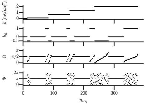
After implementing the matrix-variate Gamma approximation of Section II.3.2 in Matlab, extending the framework of Refs. Matlab_toolbox, ; Nilsson_ISMRM:2018, , we evaluated it on a healthy human-brain ‘tensor-valued’ dMRI dataset readily available online. (Szczepankiewicz_data:2019, ) This comprehensive dataset was acquired on a MAGNETOM 3T Prisma (Siemens Healthcare, Germany) using a prototype spin-echo sequence customized to support tensor-valued diffusion encoding, (Szczepankiewicz_DIVIDE:2019, ) and an echo-planar imaging (EPI) readout. (Mansfield_EPI:1977, ; Ordidge_EPI:1981, ) Its imaging parameters are , , , , , partial-, , and echo . The sequence used interleaved slice excitation, strong fat saturation, in-plane acceleration with GRAPPA reconstruction and 30 reference lines. Tensor-valued diffusion encoding was performed with numerically optimized, (Sjolund:2015, ) Maxwell-compensated, (Szczepankiewicz_Maxwell:2019, ) waveforms. The spectral tuning of these waveforms (Lundell:2019, ) is discussed in Ref. Szczepankiewicz_data:2019, . The dataset was motion- and eddy-corrected by registering the images to an extrapolated reference (Nilsson:2015, ) using Elastix. (Klein_Elastix:2010, ) Its signal-to-noise ratio (SNR) was estimated to 30 in the corona radiata using the spherically encoded diffusion signal at (see Supplemental Material of Ref. Szczepankiewicz_DIVIDE:2019, ). The overall acquisition scheme is illustrated in Figure 1.
III.2 In silico data
We evaluated the matrix-variate Gamma approximation in silico, and compared it with the covariance tensor approximation (Westin:2016, ) on the basis of estimating the statistical descriptors of interest presented in Section II.1, i.e the mean isotropic diffusivity , the normalized mean squared anisotropy and the variance of isotropic diffusivities . To that end, we used the same process as that found in Ref. Reymbaut_accuracy_precision:2020, :
-
1.
A system of interest is simulated by generating a set of ground-truth features (with the signal fraction of a given diffusion component), from which the ground-truth statistical descriptors of interest and the ground-truth set of signals , with acquisition index , are computed using the acquisition scheme of Section III.1 and a discretized version of Equation 1.
-
2.
Each signal representation is run on an identical set of signals with added Rician noise: , where and denote random numbers drawn from a normal distribution with zero mean and unit standard deviation.
-
3.
Step 2 is repeated 100 times to build up statistics on parameter estimation of , and .
In this work, we investigated a clinically relevant SNR of 30 and the ideal infinite SNR. Since the Rician bias has been shown to be relevant only when the SNR approaches five,Gudbjartsson_Patz:1995 affecting the estimation of diffusion metrics,Jones_Basser:2004 ; Gilbert:2007 ; Sotiropoulos:2013 the results presented in Section IV are identical to those obtained from signals with added Gaussian noise. While accuracy is quantified for a given estimation by the difference between the median estimation across noise realizations and the ground-truth (bias), precision is quantified by the interquartile range of estimations across noise realizations. A "good" estimation is defined as one that presents both high accuracy and high precision.
IV Results
The results presented in this section and discussed in Section V aim to evaluate the matrix-variate Gamma approximation of Section II.3.2 in vivo and in silico, thereby offering a proof of concept of the applicability of the matrix moments derived in Section II.2.3. Alternatively, these results allow to identify the nature of the diffusion information that can be captured by non-central matrix-variate Gamma distributions (as those used in the DIAMOND model (Scherrer_DIAMOND:2016, ; Scherrer_aDIAMOND:2017, ; Reymbaut_arxiv_Magic_DIAMOND:2020, )).
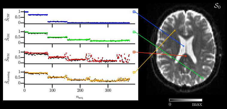
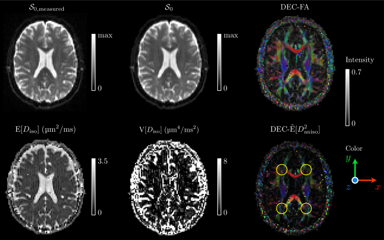
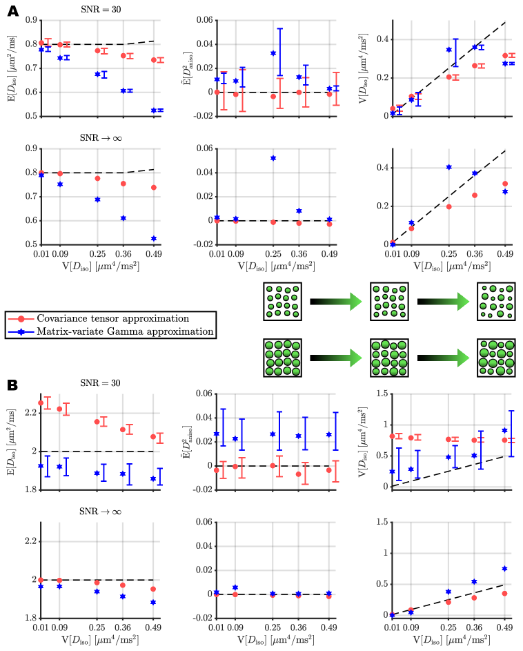
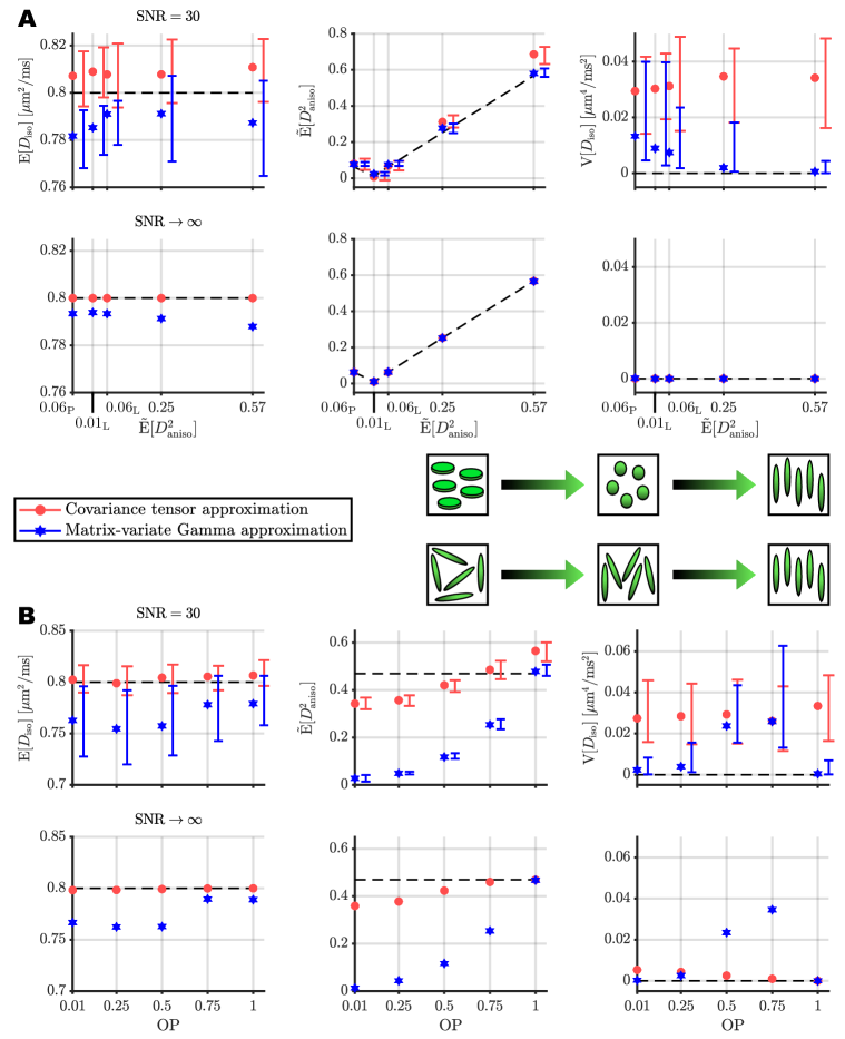
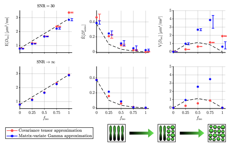
Figure 2 presents the fitted signals yielded by the matrix-variate Gamma approximation in vivo, within typical voxels associated with cerebrospinal fluid (CSF), grey matter (GM), single-fiber white matter (WM) in the corpus callosum, and crossing fibers in the anterior centrum semiovale. These fitted signals are compared with the signals measured using the acquisition scheme detailed in Section III.1. Figure 3 shows axial parameter maps of the statistical descriptors in Section II.1 estimated by the matrix-variate Gamma approximation. Unexpected discrepancies between the results of Figure 3 and the known anatomy are further investigated in silico in Figures 4, 5 and 6, which feature the statistical descriptors estimated with the matrix-variate Gamma approximation and the covariance tensor approximation of Ref. Westin:2016, in numerical systems consisting of isotropic components only, anisotropic components only, and a mixture of isotropic and anisotropic components, respectively. This in silico study followed the process detailed in Section III.2.
V Discussion
In this section, let us denote the matrix-variate Gamma approximation by "mv-Gamma" and the covariance tensor approximation by "Cov" for compactness.
As seen from Figure 2, mv-Gamma fits the dMRI signal rather adequately in various brain regions, even in areas of fiber crossings. However, Figure 3 indicates that even though this signal representation yields maps of , , and directionally encoded color (DEC) (Pajevic_Pierpaoli:1999, ) fractional anisotropy (FA) (Basser_Pierpaoli:1996, ) that are consistent with the known anatomy, it also gives anomalously large values of and a DEC normalized mean squared anisotropy that vanishes unexpectedly in fiber-crossing regions. Nevertheless, the map exhibits the contrast expected from , i.e. large values at the interface between WM and the CSF in the ventricles, and at the interface between cortical GM and the CSF surrounding the brain, and small values otherwise.
These trends are confirmed in silico in Figures 4, 5 and 6, which we first discuss. In general, the estimations of mv-Gamma and Cov share similar precision, except when estimating at high (see Figures 4 and 6), where Cov is more precise. In terms of accuracy, both signal representations share similar infinite-SNR biases in nature, although generally more pronounced for mv-Gamma. These biases persist at finite SNR, with mv-Gamma being more accurate than Cov in estimating in systems with low (see Figures 4.B and 6), in systems with high (see Figures 4.B and 6), and and in coherent (orientationally ordered) anisotropic systems (see Figure 5.A). In particular, mv-Gamma performs better than Cov in coherent anisotropic systems of high prolate anisotropy. However, while Figure 5.B demonstrates that the normalized mean squared anisotropy estimated by mv-Gamma vanishes upon reducing the orientational order parameter (Lasic:2014, ; Topgaard_liquid:2016, ) of anisotropic systems (to a greater extent compared to Cov), Figure 6 shows that the variance of isotropic diffusivities estimated by mv-Gamma can largely overshoot the ground-truth value in mixed systems with high , thereby confirming the trends seen in vivo in Figure 3.
These limitations of the matrix-variate Gamma approximation can be understood from a mathematical standpoint, in turn informing on the fundamental limitations of the nc-mv-Gamma distribution with regard to capturing intra-voxel heterogeneity. We showed in Section II.3.2 that the covariance tensor of the nc-mv-Gamma distribution (see Equations 23 and 26) can only be non-zero within its upper-left block in Mandel notation (see Section II.1). However, the other blocks of the covariance tensor, zero in the case of the nc-mv-Gamma distribution, are mostly involved in capturing the heterogeneity of orientationally dispersed voxel contents, and the heterogeneity of voxel contents simultaneously featuring variances in the trace (size) and anisotropy (shape) of the underlying diffusion tensors, as shown in Refs. Westin:2016, ; Magdoom:2020, . This explains the limitations of the matrix-variate Gamma approximation observed in Figures 3, 4, 5 and 6.
VI Conclusions
We established practical mathematical tools, the matrix moments of the diffusion tensor distribution (DTD) , that remove the fundamental barrier preventing a more widespread use of matrix-variate distributions as plausible approximations of the DTD: their intractability. Indeed, the matrix moments enable the computation of the mean diffusion tensor and covariance tensor of any matrix-variate parametric functional form chosen for the DTD, given that its moment-generating function is known. In turn, statistical descriptors of the DTD that are common to various methods can be extracted from these tensors, allowing to investigate the performance of a given functional approximation in capturing intra-voxel heterogeneity, and to compare multiple signal representations and models on the basis of estimating identical sets of descriptors.
As a proof of concept, we computed the matrix moments of the non-central matrix-variate Gamma distribution, deriving its covariance tensor for the first time. Building upon these calculations, we designed a new signal representation wherein the intra-voxel diffusion profile is described by a single non-central matrix-variate Gamma distribution: the matrix-variate Gamma approximation. This approximation fails to capture the heterogeneity arising from orientation dispersion and from simultaneous variances in the size and shape of the underlying diffusion tensors, which can be understood from the structure of the covariance tensor associated with that specific choice of parametric distribution for . However, the matrix-variate Gamma approximation performs well in orientationally ordered anisotropic systems of high prolate anisotropy, which justifies its use to describe anisotropic diffusion compartments, such as within the DIAMOND model. (Scherrer_DIAMOND:2016, ; Scherrer_aDIAMOND:2017, ; Reymbaut_arxiv_Magic_DIAMOND:2020, ) Finally, the matrix moments of the non-central matrix-variate Gamma distribution provide the DIAMOND model with fiber-specific statistical descriptors that are straightforwardly comparable to those of other fiber-specific techniques. (Assaf:2004, ; Assaf_CHARMED:2005, ; Reymbaut_arxiv_MC_DPC:2020, ) We encourage the diffusion MRI community to use these tools to experiment with other matrix-variate distributions (Gupta_Nagar_Book:2000, ) and to identify their respective advantages/limitations in capturing microstructural heterogeneity.
Acknowledgments
This work was financially supported by the Swedish Foundation for Strategic Research (ITM17-0267) and the Swedish Research Council (2018-03697).
Appendix A Validity of the DTD description
Let us discuss the validity of the DTD description found in Ref. Jian:2007, and formulated in Equation 1. This description is equivalent to considering a ‘snapshot’ of the combined non-Gaussian diffusion effects of restriction and exchange at a given observational time-scale, and approximating the signal decay as a continuous weighted sum of exponential decays. As the dMRI observational time-scale depends on the spectral content of the diffusion-encoding gradients, (Stepisnik:1981, ; Stepisnik:1985, ; Callaghan_Stepisnik:1995, ) so do the set of exponential decays estimated in Equation 1, and the measured DTD . Such time-dependent effects arise as a result of restricted diffusion (Woessner:1963, ) and exchange, (Johnson:1993, ; Li_Springer:2019, ) and have been measured in human-brain white matter, (Van:2014, ; Baron_Beaulieu:2014, ; Baron_Beaulieu:2015, ; Fieremans:2016, ; Veraart:2019, ; Lundell:2019, ; dellAcqua_ISMRM:2019, ) spinal cord (Jespersen:2018, ; Grussu:2019, ) and prostate (Lemberskiy:2017, ; Lemberskiy:2018, ) using pulse sequences specifically designed for varying the dMRI observational time-scale over extended ranges. Nevertheless, the DTD description holds for the limited range of long diffusion times probed by clinical dMRI experiments in the brain. (Clark:2001, ; Ronen:2006, ; Nilsson:2009, ; Nilsson:2013a, ; Nilsson:2013b, ; deSantis_T1:2016, ; Lampinen:2017, ; Veraart:2018, ; Grussu:2019, ; Szczepankiewicz_ISMRM:2019, )
Appendix B Validation on the matrix-variate Gaussian distribution
The expressions Equations 14 and 18 for the mean diffusion tensor and covariance tensor of are validated below by using them to retrieve the known mean tensor and covariance tensor of the mv-Gaussian distribution (Gupta_Nagar_Book:2000, ; Kollo_von_Rosen_book:2006, ) featured in Refs. Basser_Pajevic:2003, ; Pajevic_Basser:2003, ; Westin:2016, :
| (1) |
where and are arbitrary real matrices, and . To do so, we consider the moment-generating function of this distribution: (Gupta_Nagar_Book:2000, )
| (2) |
Note that similar proofs can be found in Ref. Kollo_von_Rosen_book:2006, .
B.1 Mean diffusion tensor
Using Ref. Laue_website, to compute the first-order matrix derivative of , and transposing its result according to Section II.2.2, one has
| (3) |
which immediately gives
| (4) |
using Equation 14.
B.2 Covariance tensor
The second-order matrix derivative of equals the first-order matrix derivative of Equation 3. Using the scalar product rule of Equation 12 and the fact that (Laue_website, ) , one obtains
| (5) |
which gives
| (6) |
using Equation 4, so that
| (7) |
using Equation 18.
Appendix C Proofs for the non-central matrix-variate Gamma distribution
C.1 Average diffusion tensor
Starting from the moment-generating function of the nc-mv-Gamma distribution in Equation 20, one uses Ref. Laue_website, , transposing its result according to Section II.2.2, to obtain
| (1) |
where the adjugate matrix (also called classical adjoint, or adjunct) is defined for a matrix by
| (2) |
Let us simplify the expression of Equation 1. First, one has
| (3) |
Second, Equation 3 indicates that is invertible because of the condition on ensuring the convergence of the moment-generating function Equation 20. This implies via Equation 2 that its adjugate satisfies
| (4) |
Finally, inserting Equations 3 and 4 in Equation 1 and using and yield
| (5) |
or alternatively
| (6) |
using Equation 20. Therefore, one retrieves the average diffusion tensor of the nc-mv-Gamma distribution (see Equation 22):
| (7) |
C.2 Covariance tensor
Let us write the first-order matrix derivative of Equation 6 as
| (8) |
where
| (9) |
with from Equation 7. One can now use the scalar product rule of Equation 12 to obtain
| (10) |
so that
| (11) |
and
| (12) |
Using Ref. Laue_website, and transposing its result according to Section II.2.2, one has
| (13) |
In particular,
| (14) |
Finally, combining Equations 12 and 14 yields the covariance tensor of the nc-mv-Gamma distribution (see Equation 23):
| (15) |
This proof is one of the original contributions of the present work.
References
- (1) D. Le Bihan, \htmladdnormallinkRadiology 177, 328 (1990)https://doi.org/10.1148/radiology.177.2.2217762, PMID: 2217762.
- (2) D. Le Bihan, R. Turner, P. Douek, and N. Patronas, \htmladdnormallinkAmerican Journal of Roentgenology 159, 591 (1992)https://doi.org/10.2214/ajr.159.3.1503032.
- (3) P. J. Basser, J. Mattiello, and D. LeBihan, \htmladdnormallinkBiophys J 66, 259 (1994)http://www.ncbi.nlm.nih.gov/pmc/articles/PMC1275686/.
- (4) J. Mattiello, P. Basser, and D. Lebihan, \htmladdnormallinkJournal of Magnetic Resonance, Series A 108, 131 (1994)http://www.sciencedirect.com/science/article/pii/S106418588471103X.
- (5) J. Mattiello, P. J. Basser, and D. Le Bihan, \htmladdnormallinkMagnetic Resonance in Medicine 37, 292 (1997)https://onlinelibrary.wiley.com/doi/abs/10.1002/mrm.1910370226.
- (6) D. K. Jones, Diffusion MRI (Oxford University Press, 2010).
- (7) G. J. Stanisz, G. A. Wright, R. M. Henkelman, and A. Szafer, \htmladdnormallinkMagnetic Resonance in Medicine 37, 103 (1997)http://dx.doi.org/10.1002/mrm.1910370115.
- (8) D. G. Norris, \htmladdnormallinkNMR in Biomedicine 14, 77 (2001)http://dx.doi.org/10.1002/nbm.682.
- (9) J. V. Sehy, J. J. Ackerman, and J. J. Neil, \htmladdnormallinkMagnetic Resonance in Medicine 48, 765 (2002)http://dx.doi.org/10.1002/mrm.10301.
- (10) L. Minati and W. P. Wȩglarz, \htmladdnormallinkConcepts in Magnetic Resonance Part A 30A, 278 (2007)http://dx.doi.org/10.1002/cmr.a.20094.
- (11) R. V. Mulkern, S. J. Haker, and S. E. Maier, \htmladdnormallinkMagn Reson Imaging 27, 1151 (2009)http://www.ncbi.nlm.nih.gov/pmc/articles/PMC2894527/, 19520535[pmid].
- (12) B. Jian, B. C. Vemuri, E. Özarslan, P. R. Carney, and T. H. Mareci, \htmladdnormallinkNeuroimage 37, 164 (2007)http://www.ncbi.nlm.nih.gov/pmc/articles/PMC2576290/, 17570683[pmid].
- (13) D. E. Woessner, \htmladdnormallinkThe Journal of Physical Chemistry 67, 1365 (1963)http://dx.doi.org/10.1021/j100800a509.
- (14) C. S. Johnson, \htmladdnormallinkJournal of Magnetic Resonance, Series A 102, 214 (1993)http://www.sciencedirect.com/science/article/pii/S1064185883710934.
- (15) X. Li, S. Mangia, J.-H. Lee, R. Bai, and C. S. Springer Jr, \htmladdnormallinkMagnetic Resonance in Medicine 82, 411 (2019)https://onlinelibrary.wiley.com/doi/abs/10.1002/mrm.27725.
- (16) A. L. Alexander, K. M. Hasan, M. Lazar, J. S. Tsuruda, and D. L. Parker, \htmladdnormallinkMagnetic Resonance in Medicine 45, 770 (2001)http://dx.doi.org/10.1002/mrm.1105.
- (17) D. S. Tuch et al., \htmladdnormallinkMagnetic Resonance in Medicine 48, 577 (2002)http://dx.doi.org/10.1002/mrm.10268.
- (18) D. A. Yablonskiy, G. L. Bretthorst, and J. J. Ackerman, \htmladdnormallinkMagnetic Resonance in Medicine 50, 664 (2003)http://dx.doi.org/10.1002/mrm.10578.
- (19) C. D. Kroenke, J. J. Ackerman, and D. A. Yablonskiy, \htmladdnormallinkMagnetic Resonance in Medicine 52, 1052 (2004)http://dx.doi.org/10.1002/mrm.20260.
- (20) S. N. Jespersen, C. D. Kroenke, L. Østergaard, J. J. Ackerman, and D. A. Yablonskiy, \htmladdnormallinkNeuroImage 34, 1473 (2007)http://www.sciencedirect.com/science/article/pii/S1053811906010950.
- (21) A. D. Leow et al., \htmladdnormallinkMagnetic Resonance in Medicine 61, 205 (2009)http://dx.doi.org/10.1002/mrm.21852.
- (22) O. Pasternak, N. Sochen, Y. Gur, N. Intrator, and Y. Assaf, \htmladdnormallinkMagnetic Resonance in Medicine 62, 717 (2009)https://onlinelibrary.wiley.com/doi/abs/10.1002/mrm.22055.
- (23) Y. Wang et al., \htmladdnormallinkBrain 134, 3590 (2011)http://dx.doi.org/10.1093/brain/awr307.
- (24) E. Fieremans, J. H. Jensen, and J. A. Helpern, \htmladdnormallinkNeuroImage 58, 177 (2011)http://www.sciencedirect.com/science/article/pii/S1053811911006148.
- (25) H. Zhang, T. Schneider, C. A. Wheeler-Kingshott, and D. C. Alexander, \htmladdnormallinkNeuroImage 61, 1000 (2012)http://www.sciencedirect.com/science/article/pii/S1053811912003539.
- (26) I. O. Jelescu, J. Veraart, E. Fieremans, and D. S. Novikov, \htmladdnormallinkNMR in Biomedicine 29, 33 (2016)http://dx.doi.org/10.1002/nbm.3450, NBM-15-0204.R2.
- (27) E. Kaden, N. D. Kelm, R. P. Carson, M. D. Does, and D. C. Alexander, \htmladdnormallinkNeuroImage 139, 346 (2016)http://www.sciencedirect.com/science/article/pii/S1053811916302063.
- (28) C.-F. Westin et al., \htmladdnormallinkNeuroImage 135, 345 (2016)http://www.sciencedirect.com/science/article/pii/S1053811916001488.
- (29) B. Scherrer et al., \htmladdnormallinkMagnetic Resonance in Medicine 76, 963 (2016)http://dx.doi.org/10.1002/mrm.25912.
- (30) B. Scherrer et al., Decoupling axial and radial tissue heterogeneity in diffusion compartment imaging, pp. 440–452, Information Processing in Medical Imaging (IPMI), 2017.
- (31) B. Lampinen et al., \htmladdnormallinkNeuroImage 147, 517 (2017)http://www.sciencedirect.com/science/article/pii/S105381191630670X.
- (32) M. Reisert, E. Kellner, B. Dhital, J. Hennig, and V. G. Kiselev, \htmladdnormallinkNeuroImage 147, 964 (2017)http://www.sciencedirect.com/science/article/pii/S1053811916305353.
- (33) D. S. Novikov, V. G. Kiselev, and S. N. Jespersen, \htmladdnormallinkMagnetic Resonance in Medicine 79, 3172 (2018)https://onlinelibrary.wiley.com/doi/abs/10.1002/mrm.27101.
- (34) D. S. Novikov, E. Fieremans, S. N. Jespersen, and V. G. Kiselev, \htmladdnormallinkNMR in Biomedicine 0, e3998 (2018)https://onlinelibrary.wiley.com/doi/abs/10.1002/nbm.3998.
- (35) G. Rensonnet, B. Scherrer, S. K. Warfield, B. Macq, and M. Taquet, \htmladdnormallinkMagnetic Resonance in Medicine 79, 2332 (2018)https://onlinelibrary.wiley.com/doi/abs/10.1002/mrm.26832.
- (36) S. Eriksson, S. Lasic̆, and D. Topgaard, \htmladdnormallinkJournal of Magnetic Resonance 226, 13 (2013)http://www.sciencedirect.com/science/article/pii/S1090780712003370.
- (37) C.-F. Westin et al., Measurement tensors in diffusion mri: Generalizing the concept of diffusion encoding, in Medical Image Computing and Computer-Assisted Intervention – MICCAI 2014, edited by P. Golland, N. Hata, C. Barillot, J. Hornegger, and R. Howe, pp. 209–216, Cham, 2014, MICCAI, Springer International Publishing.
- (38) S. Eriksson, S. Lasic̆, M. Nilsson, C.-F. Westin, and D. Topgaard, \htmladdnormallinkThe Journal of Chemical Physics 142, 104201 (2015)http://dx.doi.org/10.1063/1.4913502.
- (39) D. Topgaard, \htmladdnormallinkJournal of Magnetic Resonance 275, 98 (2017)http://www.sciencedirect.com/science/article/pii/S1090780716302701.
- (40) D. Topgaard, \htmladdnormallinkJournal of Magnetic Resonance 306, 150 (2019)http://www.sciencedirect.com/science/article/pii/S1090780719301491.
- (41) A. Reymbaut, P. Mezzani, J. P. de Almeida Martins, and D. Topgaard, \htmladdnormallinkNMR in Biomedicine n/a, e4267 (2020)https://onlinelibrary.wiley.com/doi/abs/10.1002/nbm.4267, e4267 nbm.4267.
- (42) D. Benjamini and P. J. Basser, \htmladdnormallinkJournal of Magnetic Resonance 271, 40 (2016)http://www.sciencedirect.com/science/article/pii/S109078071630132X.
- (43) D. Benjamini and P. J. Basser, \htmladdnormallinkMicroporous and Mesoporous Materials 269, 93 (2018)http://www.sciencedirect.com/science/article/pii/S1387181117300422, Proceedings of the 13th International Bologna Conference on Magnetic Resonance in Porous Media (MRPM13).
- (44) D. Benjamini and P. J. Basser, \htmladdnormallinkNMR in Biomedicine n/a, e4226 (2020)https://onlinelibrary.wiley.com/doi/abs/10.1002/nbm.4226.
- (45) D. Kim, E. K. Doyle, J. L. Wisnowski, J. H. Kim, and J. P. Haldar, \htmladdnormallinkMagnetic Resonance in Medicine 78, 2236 (2017)https://onlinelibrary.wiley.com/doi/abs/10.1002/mrm.26629.
- (46) D. Kim, J. L. Wisnowski, C. T. Nguyen, and J. P. Haldar, \htmladdnormallinkNMR in Biomedicine n/a, e4244 (2020)https://onlinelibrary.wiley.com/doi/abs/10.1002/nbm.4244.
- (47) J. P. de Almeida Martins and D. Topgaard, \htmladdnormallinkPhys. Rev. Lett. 116, 087601 (2016)https://link.aps.org/doi/10.1103/PhysRevLett.116.087601.
- (48) J. P. de Almeida Martins and D. Topgaard, \htmladdnormallinkScientific Reports 8, 2488 (2018)https://doi.org/10.1038/s41598-018-19826-9.
- (49) D. Topgaard, \htmladdnormallinkNMR in Biomedicine 32, e4066 (2019)https://onlinelibrary.wiley.com/doi/abs/10.1002/nbm.4066.
- (50) J. P. de Almeida Martins et al., \htmladdnormallinkMagnetic Resonance 1, 27 (2020)https://www.magn-reson.net/1/27/2020/.
- (51) J. H. Jensen, J. A. Helpern, A. Ramani, H. Lu, and K. Kaczynski, \htmladdnormallinkMagnetic Resonance in Medicine 53, 1432 (2005)http://dx.doi.org/10.1002/mrm.20508.
- (52) V. G. Kiselev, The Cumulant Expansion: An Overarching Mathematical Framework For Understanding Diffusion NMR (Oxford University Press, Oxford, UK, 2012), .
- (53) R. Nicolas, I. Sibon, and B. Hiba, \htmladdnormallinkMagnetic resonance insights 8, 11 (2015)https://europepmc.org/articles/PMC4468950.
- (54) V. Mohanty, E. T. McKinnon, J. A. Helpern, and J. H. Jensen, \htmladdnormallinkMagnetic Resonance Imaging 48, 80 (2018)http://www.sciencedirect.com/science/article/pii/S0730725X17303016.
- (55) B. Håkansson, M. Nydén, and O. Söderman, Colloid and Polymer Science 278, 399 (2000).
- (56) N. H. Williamson, M. Nydén, and M. Röding, \htmladdnormallinkJournal of Magnetic Resonance 267, 54 (2016)http://www.sciencedirect.com/science/article/pii/S1090780716300088.
- (57) M. Röding et al., \htmladdnormallinkJournal of magnetic resonance 222, 105—111 (2012)https://doi.org/10.1016/j.jmr.2012.07.005.
- (58) S. Lasic̆, F. Szczepankiewicz, S. Eriksson, M. Nilsson, and D. Topgaard, \htmladdnormallinkFrontiers in Physics 2, 11 (2014)http://journal.frontiersin.org/article/10.3389/fphy.2014.00011.
- (59) Y. Assaf, R. Z. Freidlin, G. K. Rohde, and P. J. Basser, \htmladdnormallinkMagnetic Resonance in Medicine 52, 965 (2004)http://dx.doi.org/10.1002/mrm.20274.
- (60) Y. Assaf and P. J. Basser, \htmladdnormallinkNeuroImage 27, 48 (2005)http://www.sciencedirect.com/science/article/pii/S1053811905002259.
- (61) Y. Assaf, T. Blumenfeld-Katzir, Y. Yovel, and P. J. Basser, \htmladdnormallinkMagnetic Resonance in Medicine 59, 1347 (2008)http://dx.doi.org/10.1002/mrm.21577.
- (62) S. Jbabdi, S. N. Sotiropoulos, A. M. Savio, M. Graña, and T. E. J. Behrens, \htmladdnormallinkMagnetic Resonance in Medicine 68, 1846 (2012)http://dx.doi.org/10.1002/mrm.24204.
- (63) L. Ning, M. Nilsson, S. Lasič, C.-F. Westin, and Y. Rathi, \htmladdnormallinkThe Journal of Chemical Physics 148, 074109 (2018)https://doi.org/10.1063/1.5014044.
- (64) L. Ning, B. Gagoski, F. Szczepankiewicz, C. Westin, and Y. Rathi, \htmladdnormallinkIEEE Transactions on Medical Imaging 39, 668 (2020)https://ieeexplore.ieee.org/document/8792128.
- (65) R. J. Muirhead, Aspects of Multivariate Statistical Theory (John Wiley and Sons Ltd., Hoboken, New Jersey, 1982).
- (66) A. K. Guptar and D. K. Nagar, Matrix Variate Distributions (Chapman and Hall/CRC, Boca Raton, Florida, 2000).
- (67) T. H. Anderson, An Introduction to Multivariate Statistical Analysis (Third Edition, John Wiley and Sons Ltd., Hoboken, New Jersey, 2003).
- (68) J.-D. Tournier, F. Calamante, D. G. Gadian, and A. Connelly, \htmladdnormallinkNeuroImage 23, 1176 (2004)http://www.sciencedirect.com/science/article/pii/S1053811904004100.
- (69) J.-D. Tournier, F. Calamante, and A. Connelly, \htmladdnormallinkNeuroImage 35, 1459 (2007)http://www.sciencedirect.com/science/article/pii/S1053811907001243.
- (70) P. J. Basser and S. Pajevic, \htmladdnormallinkIEEE Transactions on Medical Imaging 22, 785 (2003)https://ieeexplore.ieee.org/document/1216202.
- (71) S. Pajevic and P. J. Basser, \htmladdnormallinkJournal of Magnetic Resonance 161, 1 (2003)http://www.sciencedirect.com/science/article/pii/S1090780702001787.
- (72) A. Reymbaut et al., \htmladdnormallinkarXiv e-prints (2020)https://arxiv.org/abs/2004.07340, 2004.07340.
- (73) G. Parker et al., \htmladdnormallinkNeuroImage 65, 433 (2013)http://www.sciencedirect.com/science/article/pii/S1053811912010257.
- (74) C. M. Tax, B. Jeurissen, S. B. Vos, M. A. Viergever, and A. Leemans, \htmladdnormallinkNeuroImage 86, 67 (2014)http://www.sciencedirect.com/science/article/pii/S1053811913008367.
- (75) K. N. Magdoom, S. Pajevic, G. Dario, and P. J. Basser, \htmladdnormallinkbioRxiv (2020)https://www.biorxiv.org/content/early/2020/05/02/2020.05.01.071118.
- (76) A. Reymbaut et al., \htmladdnormallinkarXiv e-prints (2020)https://arxiv.org/abs/2004.08626, 2004.08626.
- (77) T. Kollo and D. von Rosen, Advanced Multivariate Statistics with MatricesMathematics and Its Applications (Springer Netherlands, 2006).
- (78) U. Haeberlen, High resolution NMR in solids : selective averaging (Academic Press, New York, 1976).
- (79) M. Lawrenz, M. A. Koch, and J. Finsterbusch, \htmladdnormallinkJournal of Magnetic Resonance 202, 43 (2010)http://www.sciencedirect.com/science/article/pii/S1090780709002717.
- (80) S. N. Jespersen, H. Lundell, C. K. Sønderby, and T. B. Dyrby, \htmladdnormallinkNMR in Biomedicine 26, 1647 (2013)http://dx.doi.org/10.1002/nbm.2999.
- (81) N. Shemesh et al., \htmladdnormallinkMagnetic Resonance in Medicine 75, 82 (2016)https://onlinelibrary.wiley.com/doi/abs/10.1002/mrm.25901.
- (82) A. Ianuş et al., \htmladdnormallinkNeuroImage 183, 934 (2018)http://www.sciencedirect.com/science/article/pii/S1053811918307328.
- (83) F. Szczepankiewicz et al., \htmladdnormallinkNeuroImage 104, 241 (2015)http://www.sciencedirect.com/science/article/pii/S105381191400799X.
- (84) F. Szczepankiewicz et al., \htmladdnormallinkNeuroImage 142, 522 (2016)http://www.sciencedirect.com/science/article/pii/S1053811916303457.
- (85) J. Mandel, \htmladdnormallinkInternational Journal of Solids and Structures 1, 273 (1965)http://www.sciencedirect.com/science/article/pii/002076836590034X.
- (86) Matrix calculus, wikipedia, https://en.wikipedia.org/wiki/Matrix_calculus, Accessed: 2020-05-20.
- (87) H. Turnbull, Proceedings of the Edinburgh Mathematical Society 1, 111 (1928).
- (88) H. Turnbull, Proceedings of the Edinburgh Mathematical Society 2, 33 (1930).
- (89) H. Turnbull, Proceedings of the Edinburgh Mathematical Society 2, 256 (1931).
- (90) P. S. Dwyer and M. MacPhail, The annals of mathematical statistics 19, 517 (1948).
- (91) S. M. Selby and R. C. Weast, Handbook of tables for mathematics (Chemical Rubber Company, 1967).
- (92) E. C. MacRae, The Annals of Statistics 2, 337 (1974).
- (93) J. Magnus and H. Neudecker, Matrix Differential Calculus with Applications in Statistics and Econometrics (Revised Edition) (John Wiley & Sons Ltd, 1999).
- (94) J. R. Magnus, \htmladdnormallinkJournal of Multivariate Analysis 101, 2200 (2010)http://www.sciencedirect.com/science/article/pii/S0047259X10001120.
- (95) S. Laue, M. Mitterreiter, and J. Giesen, Computing higher order derivatives of matrix and tensor expressions, in Proceedings of the 32nd International Conference on Neural Information Processing Systems, edited by S. Bengio et al., NIPS’18, p. 2755–2764, Red Hook, NY, USA, 2018, 32nd International Conference on Neural Information Processing Systems, Curran Associates Inc.
- (96) Matrix calculus, http://matrixcalculus.org, Accessed: 2020-05-20.
- (97) J. Brewer, \htmladdnormallinkIEEE Transactions on Circuits and Systems 25, 772 (1978)https://ieeexplore.ieee.org/abstract/document/1084534.
- (98) N. J. Higham, \htmladdnormallinkLinear Algebra and its Applications 103, 103 (1988)http://www.sciencedirect.com/science/article/pii/0024379588902236.
- (99) M. Nilsson, F. Szczepankiewicz, and D. Topgaard, Matlab code for multidimensional diffusion mri, https://github.com/daniel-topgaard/md-dmri, 2018, Accessed: 2020-05-20.
- (100) M. Nilsson et al., An open-source framework for analysis of multidimensional diffusion mri data implemented in matlab, Proc Intl Soc Mag Reson Med, 2018.
- (101) F. Szczepankiewicz, S. Hoge, and C.-F. Westin, \htmladdnormallinkData in Brief 25, 104208 (2019)http://www.sciencedirect.com/science/article/pii/S2352340919305621.
- (102) F. Szczepankiewicz, J. Sjölund, F. Ståhlberg, J. Lätt, and M. Nilsson, \htmladdnormallinkPLOS ONE 14, 1 (2019)https://doi.org/10.1371/journal.pone.0214238.
- (103) P. Mansfield, \htmladdnormallinkJournal of Physics C: Solid State Physics 10, L55 (1977)https://doi.org/10.1088%2F0022-3719%2F10%2F3%2F004.
- (104) R. J. Ordidge, P. Mansfield, and R. E. Coupland, \htmladdnormallinkThe British Journal of Radiology 54, 850 (1981)https://doi.org/10.1259/0007-1285-54-646-850.
- (105) J. Sjölund et al., \htmladdnormallinkJournal of Magnetic Resonance 261, 157 (2015)http://www.sciencedirect.com/science/article/pii/S1090780715002451.
- (106) F. Szczepankiewicz, C.-F. Westin, and M. Nilsson, \htmladdnormallinkMagnetic Resonance in Medicine 82, 1424 (2019)https://onlinelibrary.wiley.com/doi/abs/10.1002/mrm.27828.
- (107) H. Lundell et al., \htmladdnormallinkScientific Reports 9, 9026 (2019)https://doi.org/10.1038/s41598-019-45235-7.
- (108) M. Nilsson, F. Szczepankiewicz, D. van Westen, and O. Hansson, \htmladdnormallinkPLOS ONE 10, 1 (2015)https://doi.org/10.1371/journal.pone.0141825.
- (109) S. Klein, M. Staring, K. Murphy, M. A. Viergever, and J. P. W. Pluim, IEEE Transactions on Medical Imaging 29, 196 (2010).
- (110) H. Gudbjartsson and S. Patz, \htmladdnormallinkMagnetic Resonance in Medicine 34, 910 (1995)https://onlinelibrary.wiley.com/doi/abs/10.1002/mrm.1910340618.
- (111) D. K. Jones and P. J. Basser, \htmladdnormallinkMagnetic Resonance in Medicine 52, 979 (2004)https://onlinelibrary.wiley.com/doi/abs/10.1002/mrm.20283.
- (112) G. Gilbert, D. Simard, and G. Beaudoin, IEEE Transactions on Medical Imaging 26, 1428 (2007).
- (113) S. N. Sotiropoulos et al., \htmladdnormallinkMagnetic Resonance in Medicine 70, 1682 (2013)https://onlinelibrary.wiley.com/doi/abs/10.1002/mrm.24623.
- (114) S. Pajevic and C. Pierpaoli, \htmladdnormallinkMagnetic Resonance in Medicine 42, 526 (1999)https://onlinelibrary.wiley.com/doi/abs/10.1002/%28SICI%291522-2594%28199909%2942%3A3%3C526%3A%3AAID-MRM15%3E3.0.CO%3B2-J.
- (115) P. J. Basser and C. Pierpaoli, \htmladdnormallinkJournal of Magnetic Resonance, Series B 111, 209 (1996)http://www.sciencedirect.com/science/article/pii/S1064186696900862.
- (116) D. Topgaard, \htmladdnormallinkPhys. Chem. Chem. Phys. 18, 8545 (2016)http://dx.doi.org/10.1039/C5CP07251D.
- (117) J. Stepišnik, \htmladdnormallinkPhysica B+C 104, 350 (1981)http://www.sciencedirect.com/science/article/pii/0378436381901820.
- (118) J. Stepišnik, \htmladdnormallinkProgress in Nuclear Magnetic Resonance Spectroscopy 17, 187 (1985)http://www.sciencedirect.com/science/article/pii/007965658580008X.
- (119) P. T. Callaghan and J. Stepišnik, \htmladdnormallinkJournal of Magnetic Resonance 117, 118 (1995)https://www.sciencedirect.com/science/article/abs/pii/S1064185885799597?via%3Dihub.
- (120) A. T. Van, S. J. Holdsworth, and R. Bammer, \htmladdnormallinkMagnetic Resonance in Medicine 71, 83 (2014)https://onlinelibrary.wiley.com/doi/abs/10.1002/mrm.24632.
- (121) C. A. Baron and C. Beaulieu, \htmladdnormallinkMagnetic Resonance in Medicine 72, 726 (2014)https://onlinelibrary.wiley.com/doi/abs/10.1002/mrm.24987.
- (122) C. A. Baron et al., \htmladdnormallinkStroke 46, 2136 (2015)https://www.ahajournals.org/doi/abs/10.1161/STROKEAHA.115.008815.
- (123) E. Fieremans et al., \htmladdnormallinkNeuroImage 129, 414 (2016)http://www.sciencedirect.com/science/article/pii/S1053811916000240.
- (124) J. Veraart, E. Fieremans, and D. S. Novikov, \htmladdnormallinkNeuroImage 185, 379 (2019)http://www.sciencedirect.com/science/article/pii/S1053811918319475.
- (125) F. Dell’Acqua et al., Temporal diffusion ratio (TDR): A diffusion mri technique to map the fraction and spatial distribution of large axons in the living human brain, International Society for Magnetic Resonance Imaging (ISMRM), 2019.
- (126) S. N. Jespersen, J. L. Olesen, B. Hansen, and N. Shemesh, \htmladdnormallinkNeuroImage 182, 329 (2018)http://www.sciencedirect.com/science/article/pii/S1053811917306869, Microstructural Imaging.
- (127) F. Grussu et al., \htmladdnormallinkMagnetic Resonance in Medicine 81, 1247 (2019)https://onlinelibrary.wiley.com/doi/abs/10.1002/mrm.27463.
- (128) G. Lemberskiy et al., \htmladdnormallinkInvestigative Radiology 52, 405 (2017)https://journals.lww.com/investigativeradiology/Fulltext/2017/07000/Time_Dependent_Diffusion_in_Prostate_Cancer.3.aspx.
- (129) G. Lemberskiy et al., \htmladdnormallinkFrontiers in Physics 6, 91 (2018)https://www.frontiersin.org/article/10.3389/fphy.2018.00091.
- (130) C. A. Clark, M. Hedehus, and M. E. Moseley, \htmladdnormallinkMagnetic Resonance in Medicine 45, 1126 (2001)http://dx.doi.org/10.1002/mrm.1149.
- (131) I. Ronen, S. Moeller, K. Ugurbil, and D.-S. Kim, \htmladdnormallinkMagnetic Resonance Imaging 24, 61 (2006)http://www.sciencedirect.com/science/article/pii/S0730725X05003279.
- (132) M. Nilsson et al., \htmladdnormallinkMagnetic Resonance Imaging 27, 176 (2009)http://www.sciencedirect.com/science/article/pii/S0730725X08002014.
- (133) M. Nilsson et al., \htmladdnormallinkMagnetic Resonance in Medicine 69, 1572 (2013)http://dx.doi.org/10.1002/mrm.24395.
- (134) M. Nilsson, D. van Westen, F. Ståhlberg, P. C. Sundgren, and J. Lätt, \htmladdnormallinkMagnetic Resonance Materials in Physics, Biology and Medicine 26, 345 (2013)https://doi.org/10.1007/s10334-013-0371-x.
- (135) S. de Santis, Y. Assaf, B. Jeurissen, D. K. Jones, and A. Roebroeck, \htmladdnormallinkNeuroImage 141, 133 (2016)http://www.sciencedirect.com/science/article/pii/S1053811916303445.
- (136) B. Lampinen et al., \htmladdnormallinkMagnetic Resonance in Medicine 77, 1104 (2017)http://dx.doi.org/10.1002/mrm.26195.
- (137) J. Veraart, D. S. Novikov, and E. Fieremans, \htmladdnormallinkNeuroImage 182, 360 (2018)http://www.sciencedirect.com/science/article/pii/S1053811917307784.
- (138) F. Szczepankiewicz et al., \htmladdnormallinkProc Intl Soc Mag Reson Med 27, 0223 (2019)https://cds.ismrm.org/protected/19MPresentations/abstracts/0223.html.