The analysis of restricted five–body problem within frame of variable mass

Abstract

In the framework of restricted five bodies problem, the existence and stability of the libration points are explored and analysed numerically, under the effect of non–isotropic mass variation of the fifth body (test particle or infinitesimal body). The evolution of the positions of these points and the possible regions of motion are illustrated, as a function of the perturbation parameter. We perform a systematic investigation in an attempt to understand how the perturbation parameter due to variable mass of the fifth body, affects the positions, movement and stability of the libration points. In addition, we have revealed how the domain of the basins of convergence associated with the libration points are substantially influenced by the perturbation parameter.

1 Introduction

The $N-$body problem is not only fascinating but also presents an interesting challenge to the researchers and scientists. In general the space missions could be designed within frame of the $N-$body problem, which can be reduced to three, four or five–body problem in some cases, etc. The dynamical system of restricted five–body problem has a great significance in celestial mechanics. So many researchers over the world are currently interested in studying and solving aforesaid problem, i.e., the restricted five–body problem with various perturbation forces. The restricted five–body problem primarily takes into account a fifth body referred as the test particle with negligible mass, which does not influence the motion of four primaries moving in circular orbits around their common center of mass. This problem is a simple extension of four–body problem. Some of work are available on the planar central configuration of $N-$bodies with $N=4,5$ and $7$, see for details esgl , PK07 , jaume .

The history of restricted problem of $N-$bodies start with Euler and Lagrange where they discussed the restricted problem for $N=3$. The collinear central configuration was introduced by Euler, whereas triangular central configuration was introduced by Lagrange. The central problem deals with determination of the geometric configuration for $N-$point masses interacting in gravitational fields. Till date an analytical solution for this $N-$body $(N\geq 3)$ problem is not available. Many results have been published and put forward by a number of researchers with various perturbations like oblateness or triaxial of the primaries(e.g.,Abouelmagd and Guirao (2016) Abouelmagd et al (2015b), Abouelmagd et al (2015), Elshaboury et al. (2016)) the radiation pressure effects (e.g., Suraj et al (2018d)), effect of the Coriolis and centrifugal forces (e.g., BH78 ), the restricted three body problem with variable mass (e.g., Shrivastava and Ishwar (1983), Das et al. (1988), Abouelmagd and Mostafa (2015)) and many others in the context of restricted three–body problem (e.g., Abouelmagd et al (2014b), Abouelmagd et al (2014a), WHH ).

In spite of all these facts, the problem involving $N\geq 3$ is still interesting and open burning topic of research. The various surprising results in the study of restricted problem of three bodies paved the path and motivated researchers to extend this dynamical model into restricted four and five–body problem. However, as we move on the restricted four and five–body problem from the restricted three–body problem, the complications and challenges increase manifold. Some of the notable study in the context of restricted four–body problem with various perturbations are (e.g., SAP17 , Suraj et al. (2018a)), with oblateness of the primaries (e.g., SAA18 , Suraj et al. (2017b)), effect of the Coriolis and centrifugal forces (e.g., SV15 , SAA17 , Aggarwal et al. (2018)), effect of variable mass (e.g., MAB16 , Mittal et al. (2018)).

The restricted problem of five bodies was introduced by oll88 , where he discussed the motion of the fifth body of negligible mass, in comparison to remaining four bodies. His mathematical model was described as follows: three equal masses primaries moving around their gravitational center in circular orbit under their mutual gravitational attraction were taken on the same plane whereas, a mass of $\beta>0$ times, the mass of one of the three primary bodies is supposed at the center of mass. The presented mathematical model of five–body problem reduced to the restricted four–body problem for particular value of $\beta=0$. His study unveils the fact that there exist nine libration points in total in which three are stable for $\beta>43.18$, on the other hand all these nine libration points are linearly unstable for smaller values of $\beta$.

In continuation of Ollöngren, PK07 have introduced the effect of radiation pressure due to some or all of the four primaries and explored numerically that the number of collinear libration points of this dynamical system depends on mass parameter, as well as on the radiation pressure. Most recently, ZS17 have investigated the basins of convergence associated with the libration points by using multivariate version of Newton–Raphson iterative scheme in the restricted five–body problem. The numerical simulation has been presented to explore the behaviour that how the libration points (which act as attractors) of the system attract the initial conditions, always referred as nodes lying on the configuration plane and constitute a domain of basins of convergence. The author has emphasised that the geometry of the basins of convergence is highly influenced by the mass parameter.

The aforementioned literatures provide us an idea to introduce the effect of variable mass in the frame of five–body problem. The effects of variable mass in three or four–body problem have explored various new results and facts, therefore, the study of the effect of variable mass within the frame of five–body problem is novel and worth study in spite of lots of complications.

The manuscript is prepared as follows: A literature review within frame of $N-$bdy problem is stated in Section 1, but the most important properties and equations of motion for five–body problem are discussed in Section 2. In Section 3, the main numerical results regarding the parametric evolution of the positions of libration points are presented, while in Section 4 the stability of these points is studied. The most intrinsic properties of the dynamical system of restricted five–body problem have been revealed by using the Newton-Raphson basins of convergence in Section 5. Finally, discussion and conclusion are drew in Section 6.

2 Structures of equations of motion

The dynamical system of studying is the circular restricted five–body problem. This problem consists of four primaries $P_{i}$, $i=0,1,2,3$ which move in circular orbit around their common center of mass. We, further, supposed that the fifth body whose mass is too small in comparison to masses of the primaries, and its mass is not constant on the contrary its mass varies with respect to time. In this context the fifth body (test particle) dose not affect on the motion of the four primaries.

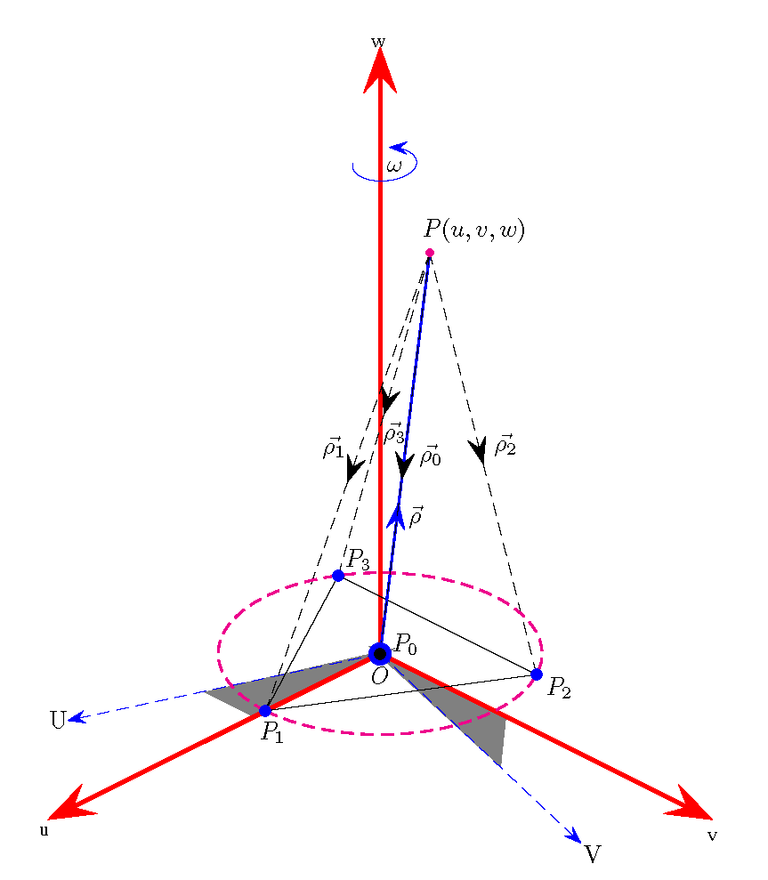
Figure 1: The planar configuration of the circular restricted five–body problem. The blue dots shows the positions of the four primary bodies.

In the planar motion of the test particle, we choose the rotating frame of reference where the origin coincides with the center of mass of the primaries. The positions of the center of the primaries are: $(u_{0},v_{0})=$$(0,0)$, $(u_{1},v_{1},w_{1})=$$(1/\sqrt{3},0,0)$, $(u_{2},v_{2},w_{2})=$$(-1/2\sqrt{3},1/2,0)$, and $(u_{3},v_{3},w_{3})=$ $(-1/2\sqrt{3},-1/2,0)$, while the dimensionless masses of the primaries are $m_{0}=\beta m^{*}$, $m_{1}=m_{2}=m_{3}=m^{*}=1$. In addition, the three primaries with mass $m^{*}$ are situated at the vertices of an equilateral triangle whose side is unity, while the fourth primary, with mass $\beta m^{*}$, is situated at the center of the equilateral triangle.

According to oll88 , and ZS17 , in the synodic coordinates system, the effective potential function of the circular restricted five–body problem is given as:

$$\Omega^{*}=k\sum\limits_{i=0}^{3}\frac{m_{i}}{\rho_{i}}+\frac{1}{2}\left(u^{2}+v^{2}\right),$$ (1)

where $k=1/3(1+\beta\sqrt{3})$ and

$$\rho_{i} =\sqrt{(u-u_{i})^{2}+(v-v_{i})^{2}+(w-w_{i})^{2}},i=0,1,2,3.$$

are the distances between the respective primaries and test particle.

The equations of motion for a test particle, with dimensionless variables in a rotating coordinates system in which the primary $m_{1}$ is fixed on the Ou–axis, are read as:

$$\left(\ddot{u}-2\dot{v}\right)+n\frac{\dot{m}}{m}\left(\dot{u}-v\right) =\Omega^{*}_{u},$$ (2a)

$$\left(\ddot{v}+2\dot{u}\right)+n\frac{\dot{m}}{m}\left(\dot{v}+u\right) =\Omega^{*}_{v},$$ (2b)

$$\ddot{w}+n\frac{\dot{m}}{m}\dot{w} =\Omega^{*}_{w},$$ (2c)

where $\Omega^{*}_{u},$ $\Omega^{*}_{v}$ and $\Omega^{*}_{w}$ are partial derivatives of the effective potential given in Eq. (1).

Moreover, the Jeans’ law states that $dm/dt=-\alpha m^{s}$, where $\alpha$ is a constant coefficient and $0.4\leq s\leq 4.4$. Acquainting the space–time transformations which read as:

$$u=\gamma^{-q}x,\,\,v=\gamma^{-q}y,\,\,w=\gamma^{-q}z,\,\,dt=\gamma^{-k}d\tau,$$

where $\gamma=m/m_{init}$, $m_{init}$ is the mass of the test particle at the initial time i.e., $t=0$. Adopting the procedure given by Shrivastava and Ishwar (1983) and Das et al. (1988), to free the equations of motion of the test particle from the factor which depends upon the variation of mass, it is sufficient to set $s=1,q=\frac{1}{2},k=0$. Therefore, the components of velocity and acceleration can be read as:

$$\gamma^{\frac{1}{2}}\dot{u} = x^{{}^{\prime}}+\frac{1}{2}\alpha x,$$ (3a)

$$\gamma^{\frac{1}{2}}\dot{v} = y^{{}^{\prime}}+\frac{1}{2}\alpha y,$$ (3b)

$$\gamma^{\frac{1}{2}}\dot{w} = z^{{}^{\prime}}+\frac{1}{2}\alpha z,$$ (3c)

$$\gamma^{\frac{1}{2}}\ddot{u} = x^{{}^{\prime\prime}}+\alpha x^{{}^{\prime}}+\frac{1}{4}\alpha^{2}x,$$ (3d)

$$\gamma^{\frac{1}{2}}\ddot{v} = y^{{}^{\prime\prime}}+\alpha y^{{}^{\prime}}+\frac{1}{4}\alpha^{2}y,$$ (3e)

$$\gamma^{\frac{1}{2}}\ddot{w} = z^{{}^{\prime\prime}}+\alpha z^{{}^{\prime}}+\frac{1}{4}\alpha^{2}z,$$ (3f)

where

$$(^{\prime})=\frac{d}{d\tau},\quad(.)=\frac{d}{dt},\quad\text{and}\quad\frac{d}{dt}=\frac{d}{d\tau}.$$

Using Eqs. (3a–3f) into Eqs. (2a–2c), we get

$$\left(\ddot{x}-2\dot{y}\right)-\alpha(n-1)\dot{x}+\alpha(n-1)y =\Omega^{**}_{x},$$ (4a)

$$\left(\ddot{y}+2\dot{x}\right)-\alpha(n-1)\dot{y}-\alpha(n-1)x =\Omega^{**}_{y},$$ (4b)

$$\ddot{z}-\alpha(n-1)\dot{z} =\Omega^{**}_{z},$$ (4c)

where

$$\Omega^{**} =k\gamma^{\frac{3}{2}}\sum\limits_{i=0}^{3}\frac{m_{i}}{r_{i}}+\frac{\alpha^{2}}{8}(2n-1)\big{(}x^{2}+y^{2}+z^{2}\big{)}+\frac{1}{2}\Big{(}x^{2}+y^{2}\Big{)},$$

$$r_{i} =\sqrt{(x-x_{i})^{2}+(y-y_{i})^{2}+(z-z_{i})^{2}},$$

$$x_{0} =0,x_{1}=\frac{\gamma^{\frac{1}{2}}}{\sqrt{3}}=-2x_{2}=-2x_{3},$$

$$y_{0} =y_{1}=0,y_{2}=\frac{\gamma^{\frac{1}{2}}}{2}=-y_{3},$$

$$z_{i} =0,i=0,1,2,3.$$

The Eqs. (4a–4c) describe the equations of motion of the fifth body where the variation of mass of the fifth particle is non-isotropic. Further, it is supposed that the variation of mass is from the entire surface (i.e., from $n$ distinct points), and the ejaculation from or fall of masses to the surface has zero momentum in the circular restricted five-body problem. Furthermore, when we consider the case that the variation of the mass emanate from one point only (i.e., $n=1$), thus, the equations of motion given by Eqs. (4a–4c) read as:

$$\ddot{x}-2\dot{y} =\Omega_{x},$$ (5a)

$$\ddot{y}+2\dot{x} =\Omega_{y},$$ (5b)

$$\ddot{z} =\Omega_{z},$$ (5c)

where

$$\Omega =k\gamma^{\frac{3}{2}}\sum\limits_{i=0}^{3}\frac{m_{i}}{r_{i}}+\frac{\alpha^{2}}{8}\left(x^{2}+y^{2}+z^{2}\right)+\frac{1}{2}\Big{(}x^{2}+y^{2}\Big{)},$$

$$\Omega_{x} =-k\gamma^{\frac{3}{2}}\sum_{i=0}^{3}\frac{m_{i}\tilde{x}_{i}}{r_{i}^{3}}+\Big{(}1+\frac{\alpha^{2}}{4}\Big{)}x,$$

$$\Omega_{y} =-k\gamma^{\frac{3}{2}}\sum_{i=0}^{3}\frac{m_{i}\tilde{y}_{i}}{r_{i}^{3}}+\Big{(}1+\frac{\alpha^{2}}{4}\Big{)}y,$$

$$\Omega_{z} =-k\gamma^{\frac{3}{2}}\sum_{i=0}^{3}\frac{m_{i}\tilde{z}_{i}}{r_{i}^{3}}+\frac{\alpha^{2}}{4}z,$$

$$\tilde{x}_{i} =x-x_{i},\quad\tilde{y}_{i}=y-y_{i},\quad\tilde{z}_{i}=z-z_{i}.$$

In the same vein, the $2^{nd}-$order partial derivatives which will be used to discuss the linear stability of the obtained libration point can be written as:

$$\Omega_{xx} = -k\gamma^{\frac{3}{2}}\sum_{i=0}^{3}\Big{(}\frac{m_{i}}{r_{i}^{3}}-\frac{3m_{i}\tilde{x}_{i}^{2}}{r_{i}^{5}}\Big{)}+\Big{(}1+\frac{\alpha^{2}}{4}\Big{)},$$ (6a)

$$\Omega_{yy} = -k\gamma^{\frac{3}{2}}\sum_{i=0}^{3}\Big{(}\frac{m_{i}}{r_{i}^{3}}-\frac{3m_{i}\tilde{y}_{i}^{2}}{r_{i}^{5}}\Big{)}+\Big{(}1+\frac{\alpha^{2}}{4}\Big{)},$$ (6b)

$$\Omega_{zz} = -k\gamma^{\frac{3}{2}}\sum_{i=0}^{3}\Big{(}\frac{m_{i}}{r_{i}^{3}}-\frac{3m_{i}\tilde{z}_{i}^{2}}{r_{i}^{3}}\Big{)}+\frac{\alpha^{2}}{4},$$ (6c)

$$\Omega_{xy} = k\gamma^{\frac{3}{2}}\sum_{i=0}^{3}\frac{3m_{i}\tilde{x}_{i}\tilde{y}_{i}}{r_{i}^{5}}=\Omega_{yx},$$ (6d)

$$\Omega_{xz} = k\gamma^{\frac{3}{2}}\sum_{i=0}^{3}\frac{3m_{i}\tilde{x}_{i}\tilde{z}_{i}}{r_{i}^{5}}=\Omega_{zx},$$ (6e)

$$\Omega_{yz} = k\gamma^{\frac{3}{2}}\sum_{i=0}^{3}\frac{3m_{i}\tilde{y}_{i}\tilde{z}_{i}}{r_{i}^{5}}=\Omega_{zy}.$$ (6f)

3 Equilibrium points

The equilibrium point exists if and only if the following conditions hold:

$$\dot{x}=\dot{y}=\dot{z}=\ddot{x}=\ddot{y}=\ddot{z}=0.$$

Similar to the mass parameter of the classical restricted three–body problem, we can take a mass parameter $\mu=1/(1+\beta)$ to compare them. Therefore, we have $\mu\in(0,1]$ when $\beta\in[0,\infty)$.

3.1 The libration points in configuration $(x,y)-$plane

In this subsection, we restrain our analysis only to the equilibrium points which lie on the $(x,y)-$plane, when $z=0$. The associated positions $(x_{0},y_{0})$ of the libration points can easily be found by solving numerically the system of the $1^{st}-$order partial derivative equations i.e., Eqs. (7) appended below:

$$\begin{cases}\Omega_{x}(x,y,z)|_{(z=0)}=0,\\ \Omega_{y}(x,y,z)|_{(z=0)}=0.\\ \end{cases}$$ (7)

The total number of the equilibrium points location, in the circular restricted five–body problem in classical case, depend on the mass parameter $\mu$ (see ZS17 ). Moreover, the number of the libration points vary for critical value of the mass parameter(i.e., $\mu^{*}=0.98617275$). Therefore, when we have taken the mass of the test particle as variable, we will explore how the number and positions of the equilibrium points are effected by the parameters $\alpha$ as well as $\gamma$.

$\mu$	$\mu^{*}$	$\alpha$	Libration points
$(0,\mu^{*})$ and $[\mu^{*},1)$	0.95353029	2	9 and 15
$(0,\mu^{*})$ and $[\mu^{*},1)$	0.97290121	1.5	9 and 15
$(0,\mu^{*})$ and $[\mu^{*},1)$	0.98510106	0.5	9 and 15
$(0,\mu^{*})$ and $[\mu^{*},1)$	0.98617275	0	9 and 15

Table 1: The number of libration points when $\alpha$ varies.

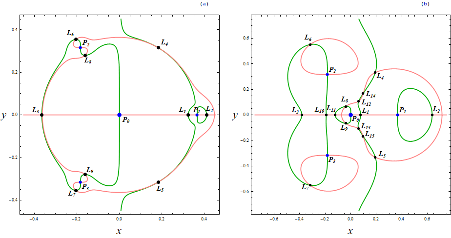
Figure 2: Positions (black dots) and numbering of the equilibrium points ($L_{i},i=1,...,9\text{or}15$) through the intersections of $\Omega_{x}=0$ (green) and $\Omega_{y}=0$ (blue), when (a–left):$\mu=0.005$, $\alpha=0.2$ and $\gamma=0.4$ (nine equilibrium points), and (b–right): $\mu=0.96353029$, $\alpha=2$ and $\gamma=0.4$ (fifteen equilibrium points). The blue dots denote the centers $(P_{i},i=0,1,2,3)$ of the primaries.

From Table (1), it is revealed that the critical value $\mu^{*}$ changes, i.e., the interval in which 9 libration points exist decreases and obviously the length of interval which contain 15 libration points increases when $\alpha$ increases.

The positions of the equilibrium points can be illustrated by the intersections of the equations $\Omega_{x}=0$, and $\Omega_{y}=0$. In Fig. 2 (a – b), we have shown how the above mentioned equations nail, in every case, the positions of the equilibrium points, for (a): $\mu=0.005$ and (b): $\mu=0.96353029$ with fixed value of $\alpha=2$ and $\gamma=0.4$. Moreover, in the corresponding panels of the figures, we depicted the numbering, $L_{i},i=1,...,9\quad\text{or}\quad 15$, of all the libration points.

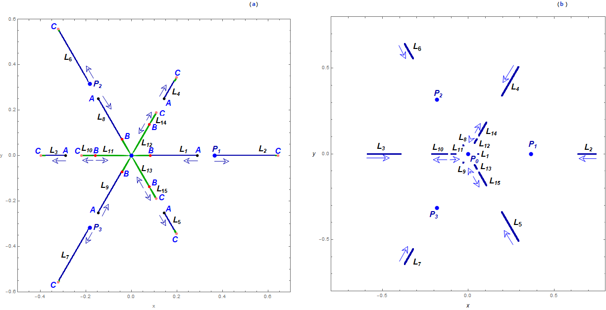
Figure 3: The parametric evolution of the positions of the libration points, $L_{i}$, $i=1,...,9\text{or}15$, in the restricted five–body problem with variable mass: (a) when $\mu\in(0,1]$. The arrows indicate the movement direction of the libration points as the value of the mass parameter increases. The big blue dots pinpoint the fixed centers of the primaries, while the small black, red and pink dots (points $A$, $B$, and $C$) correspond to $\mu\rightarrow 0$, $\mu=\mu^{*}=0.95353029$, and $\mu=1$, respectively with $\alpha=2$ and $\gamma=0.4$, (b) when $\mu=0.987$, $\gamma=0.4$, and $\alpha\in(0,2.2]$. (colour figure online).

The parametric evolution of the locations of the coplanar [i.e., on $(x,y)-$plane] equilibrium points are presented in Fig. (3), whereas in Fig. (4) positions of the out–of–plane [i.e., on the $(x,z)-$plane] libration points are illustrated. In Fig. (3 a), the movement of the position of libration points is shown for fixed value of $\alpha=2,\gamma=0.4$ and varying values of parameter $\mu\in(0,1]$, whereas in Fig. (3 b), this movement is shown for fixed value of $\mu=0.987,\gamma=0.4$ and varying values of $\alpha\in(0,2.2]$. From Fig. (3 a), we have observed that when the parameter $\mu$ is just above zero, the libration points $L_{1,6,7}$ emerged in the vicinity of primaries $P_{1,2,3}$ respectively, and the libration points $L_{1,8,9,11,12,13}$ collide with the origin for $\mu=1$. If we compare our analysis with Fig. (3) of ZS17 , it is concluded that the three libration points $L_{1,8,9}$ do not emerge in the vicinity of the primaries when the parameter $\alpha$ due to variable mass is introduced. It is also noticed that all the libration points germinates with the axes of symmetry $y=0,y=\sqrt{3\gamma}$ and $y=-\sqrt{3\gamma}$. Moreover, the movement of the positions of all libration points is same as in Fig. (3) of ZS17 .

In Fig. (3 b), we have observed that the movement of the positions of the equilibrium points $L_{2,3,4,5,6,7}$ is reversed (as these points move far from the primary $P_{0}$ along the line of symmetry when $\mu$ increases, see Fig. (3 a) and it started to move toward the primary $P_{0}$ along the line of symmetry when $\alpha$ increases. In addition, the change in the libration points $L_{1,8,9}$ is negligible whereas $L_{10,14,15}$ move away from primary $P_{0}$ as $\alpha$ increases.

3.2 Out–of–plane libration points

In this subsection, we continue our analysis with the out–of–plane equilibrium points, i.e., the libration points which lie on $(x,z)-$plane ($y=0$). By solving numerically the system of $1^{st}-$order derivative equations, with a help of Eqs. (8), we obtain

$$\begin{cases}\Omega_{x}(x,y,z)|_{(y=0)}=0,\\ \Omega_{z}(x,y,z)|_{(y=0)}=0,\end{cases}$$ (8)

we can determine the locations of the out–of–plane equilibrium points. The intersections of the equations $\Omega_{x}=0$, and $\Omega_{z}=0$ describe the locations of these equilibrium point. In Fig. (4), the parametric evolution of the locations of the libration points on $(x,z)-$plane, when $\alpha\in(0,2.2]$, is illustrated for pre defined value of the parameter $\mu=0.9862727$, $\gamma=0.4$ and varying value of $\alpha\in(0,2.2]$. As the value of the parameter $\alpha>0$ increases, a pair of symmetrical (with respect to $x-$axis) out–of–plane libration point namely $L_{z_{1}}$ and $L_{z_{2}}$ appear on the $z-$axis. In addition, these equilibrium points move towards the central primary $P_{0}$ as the parameter $\alpha$ increases. Finally, it is unveiled that the libration points always lie on coordinates axes $(x,z)$.

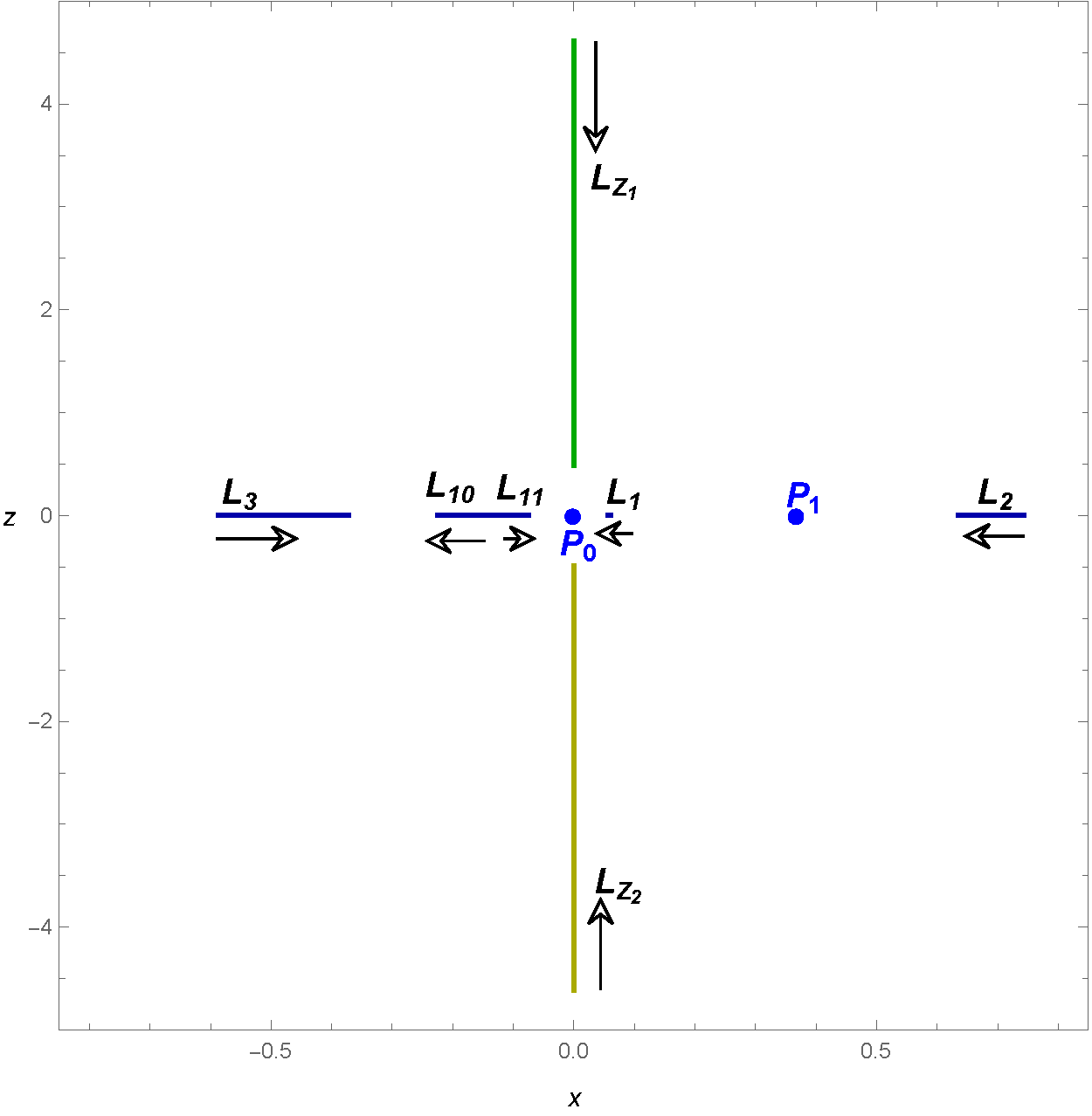
Figure 4: The parametric evolution of the positions of the out–of–plane libration points, $L_{z_{1}}$, and $L_{z_{2}}$, in the restricted five–body problem with variable mass when $\mu=0.9862727,\gamma=0.4$ and $\alpha\in(0,2.2]$. The arrows indicate the movement direction of the libration points as the value of the mass parameter increases. The big blue dots pinpoint the fixed centers of the primaries. (colour figure online).

4 Stability of libration points

The dynamical systems which describe the restricted five–body problem are developed, but they do not provide a concise characterization relating to the fifth body motion. The measurements process and the behaviour of dynamical motion of these systems are affected by the parameters variation or the state variables which give an exact definitions of the initial conditions. In addition, there is an extra difficulty to find a solution for these systems directly, for any parameter selection from a specific measurements set. Regard to the large complexity that included in these systems, our attentions are paid to linearize the dynamical system in Eqs. (5a – 5c) to obtain more simple dynamical system that can be used to underline the features of fifth body motion and its dynamical characterizations. To understand and investigate the dynamics of possible motion of the fifth body in the proximity of libration points, the equations of motion, we have linearized Eqs. (5a – 5c) along the initial state vector. Thereby, we expand their right hand-side around the equilibria points. Hence, the obtained linear system is called the variational equations. Applying the procedure of MAB16 ; Mittal et al. (2018), we shall give displacements in $(x_{0},y_{0},z_{0})$ as:

$$x=x_{0}+\epsilon_{1},\quad y=y_{0}+\epsilon_{2},\quad z=z_{0}+\epsilon_{3},(\epsilon_{1},\epsilon_{2},\epsilon_{3}<<1)$$

where $(x_{0},y_{0},z_{0})$ denote the position of equilibrium point for a fixed value of time $t$. The associated variational equations can be written as:

$$\ddot{\epsilon_{1}}-2\dot{\epsilon_{2}} = (\Omega_{xx})_{0}\epsilon_{1}+(\Omega_{xy})_{0}\epsilon_{2}+(\Omega_{xz})_{0}\epsilon_{3},$$

$$\ddot{\epsilon_{2}}+2\dot{\epsilon_{1}} = (\Omega_{yx})_{0}\epsilon_{1}+(\Omega_{yy})_{0}\epsilon_{2}+(\Omega_{yz})_{0}\epsilon_{3},$$

$$\ddot{\epsilon_{3}} = (\Omega_{zx})_{0}\epsilon_{1}+(\Omega_{zy})_{0}\epsilon_{2}+(\Omega_{zz})_{0}\epsilon_{3},$$ (9)

where the subscript ‘$0$’ in Eqs. 4 associated with the values of $2^{nd}-$order partial derivatives of $\Omega$ evaluated at the libration point $(x_{0},y_{0},z_{0})$ under consideration. The problem of constant mass can be easily obtained by taking $\alpha=0$ in the problem of variable mass.

Applying the procedure and transformations given in MAB16 ; Mittal et al. (2018), the characteristic equation of the coefficient matrix is written as

$$\lambda^{6} - 3\alpha\lambda^{5}+\Big{(}\frac{15}{4}\alpha^{2}+\phi_{1}\Big{)}\lambda^{4}-\Big{(}\frac{5}{2}\alpha^{3}+2\phi_{1}\alpha\Big{)}\lambda^{3}$$ (10)

$$+\Big{(}\frac{15}{16}\alpha^{4}+\frac{3}{2}\phi_{1}\alpha^{2}+\phi_{2}\Big{)}\lambda^{2}-\Big{(}\frac{3}{16}\alpha^{5}+\frac{1}{2}\phi_{1}\alpha^{3}$$

$$+\phi_{2}\alpha\Big{)}\lambda+\Big{(}\frac{1}{64}\alpha^{6}+\frac{1}{16}\phi_{1}\alpha^{4}+\frac{1}{4}\phi_{2}\alpha^{2}+\phi_{3}\Big{)}=0,$$

where

$$\phi_{1} = 4-(\Omega_{xx})_{0}-(\Omega_{yy})_{0}-(\Omega_{zz})_{0},$$

$$\phi_{2} = (\Omega_{xx})_{0}(\Omega_{zz})_{0}+(\Omega_{yy})_{0}(\Omega_{zz})_{0}+(\Omega_{xx})_{0}(\Omega_{yy})_{0}-4(\Omega_{zz})_{0}$$

$$-[(\Omega_{xy})_{0}]^{2}-[(\Omega_{xz})_{0}]^{2}-[(\Omega_{yz})_{0}]^{2},$$

$$\phi_{3} = -(\Omega_{xx})_{0}(\Omega_{yy})_{0}(\Omega_{zz})_{0}+(\Omega_{zz})_{0}[(\Omega_{xy})_{0}]^{2}$$

$$+(\Omega_{yy})_{0}[(\Omega_{xz})_{0}]^{2}+(\Omega_{xx})_{0}[(\Omega_{yz})_{0}]^{2}-2(\Omega_{xy})_{0}\times(\Omega_{xz})_{0}(\Omega_{yz})_{0},$$

the values of $(\Omega_{xx})_{0}$, $(\Omega_{yy})_{0}$, $(\Omega_{zz})_{0}$, $(\Omega_{xy})_{0}$, $(\Omega_{xz})_{0}$ and $(\Omega_{yz})_{0}$ are given by the Eqs. (6a – 6f).

If the exact positions of the in plane [i.e., on $(x,y)-$plane] and out–of–plane [i.e., on $(x,z)-$plane] libration points are denoted by $(x_{0},y_{0},0)$ and $(x_{0},0,z_{0})$, respectively, then we can easily decide the linear stability of these libration points by determining the nature of the roots of the characteristic equation [i.e., Eq. (10)]. We have numerically determined the linear stability of the libration points for various combination of the parameters, and found each libration point is unstable.

5 Basins of convergence

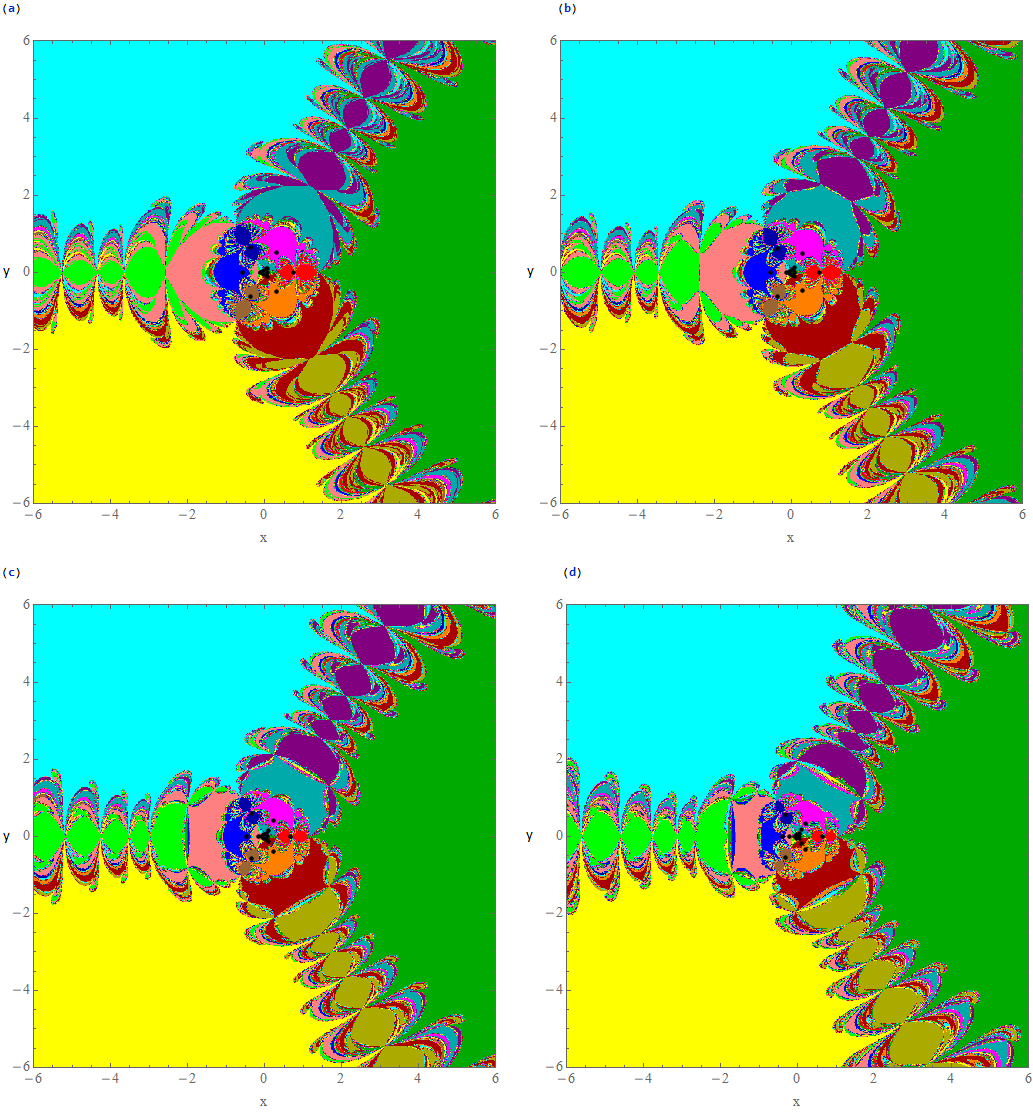
Figure 5: The basins of attraction for fixed value of $\gamma=0.4$ and $\mu=0.986173$. (a) $\alpha=0.2$; (b) $\alpha=0.75$; (c) $\alpha=1.5$; (d) $\alpha=2$. The color code for the libration points $L_{1}$,…,$L_{15}$ is as follows: $L_{1}\emph{(green)}$; $L_{2}\emph{(red)}$; $L_{3}\emph{(blue)}$; $L_{4}\emph{(magenta)}$; $L_{5}\emph{(orange)}$; $L_{6}\emph{(indigo)}$; $L_{7}\emph{(brown)}$; $L_{8}\emph{(cyan)}$; $L_{9}\emph{(yellow)}$; $L_{10}\emph{(pink)}$; $L_{11}\emph{(fluorescent green)}$; $L_{12}\emph{(purple)}$; $L_{13}\emph{(olive)}$; $L_{14}\emph{(teal)}$; $L_{15}\emph{(crimson)}$; and non–converging points (white). (colour figure online).

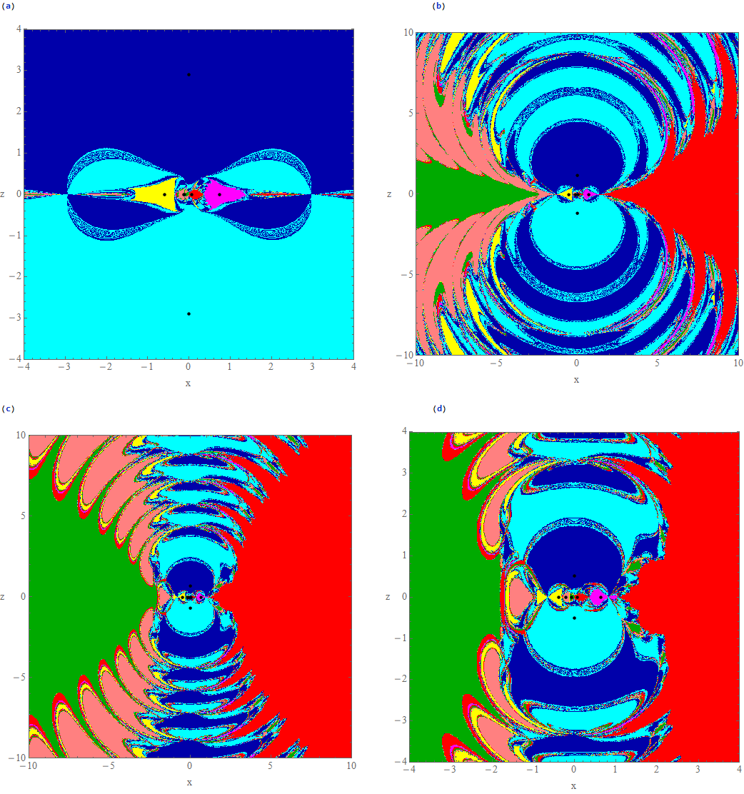
Figure 6: The out-of-plane basins of attraction for fixed value of $\gamma=0.4$ and $\mu=0.9862727$. (a) $\alpha=0.2$; (b) $\alpha=0.75$; (c) $\alpha=1.5$; (d) $\alpha=2$. The color code for the libration points is as follows: $L_{1}\emph{(red)}$; $L_{2}\emph{(magenta)}$; $L_{3}\emph{(yellow)}$; $L_{10}\emph{(pink)}$; $L_{11}\emph{(fluorescent green)}$; $L_{z_{1}}\emph{(blue)}$; $L_{z_{2}}\emph{(cyan)}$; and non-converging points (white). (colour figure online).

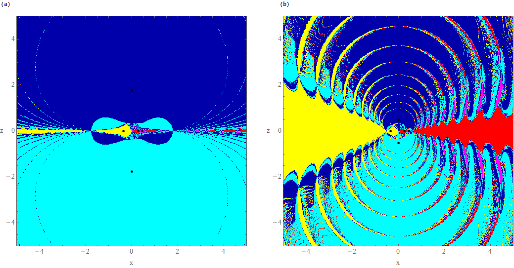
Figure 7: The out-of-plane basins of attraction for fixed value of $\gamma=0.4$ and $\mu=0.05$. (a) $\alpha=0.2$; (b) $\alpha=1.25$. The color code for the libration points is as follows: $L_{1}\emph{(red)}$; $L_{2}\emph{(magenta)}$; $L_{3}\emph{(yellow)}$; $L_{z_{1}}\emph{(blue)}$; $L_{z_{2}}\emph{(cyan)}$; and non-converging points (white). (colour figure online).

In spite of various available iterative scheme to solve the system of non–linear equations, the Newton–Raphson iterative scheme has considered as one of the most enthralled as well as precise iterative method to solve these equations. We can solve the system of multivariate functions $F(\mathbf{x})=0$ by applying the multivariate iterative scheme appended below:

$$\textbf{x}_{n+1}=\textbf{x}_{n}-{J}^{-1}f(\textbf{x}_{n}),$$ (11)

where $f(\textbf{x}_{n})$ represents the system of equations, while $J^{-1}$ represents the corresponding inverse Jacobian matrix [see Eq. (11)]. In the recent time, the study of the basins of convergence by using the multivariate version of the Newton–Raphson iterative scheme are present in various dynamical system (e.g., Suraj et al. (2018a), SZK18 , Z18 , ZSMA18 ). In our system, we have three equations, i.e., $\Omega_{x}=\Omega_{y}=\Omega_{z}=0$. It can be noticed that the Newton–Raphson iterative scheme is applicable in system of three equations but it is very complicated. Therefore, to make the iterative scheme simple, we have bifurcated our study into two part: the libration points on $(x,y)-$ plane and the out–of–plane libration points which lie on $(x,z)-$ plane. Thus, the bivariate Newton–Raphson iterative scheme can be used on the system:

$$\Omega_{x}(x,y,0) = 0,$$

$$\Omega_{y}(x,y,0) = 0.$$

Moreover, the iterative formulae for the $(x,y)$ plane can be written as:

$$x_{n+1} = x_{n}-\frac{\Omega_{x_{n}}\Omega_{y_{n}y_{n}}-\Omega_{y_{n}}\Omega_{x_{n}y_{n}}}{\Omega_{x_{n}x_{n}}\Omega_{y_{n}y_{n}}-\Omega_{x_{n}y_{n}}\Omega_{y_{n}x_{n}}},$$ (13a)

$$y_{n+1} = y_{n}+\frac{\Omega_{x_{n}}\Omega_{y_{n}x_{n}}-\Omega_{y_{n}}\Omega_{x_{n}x_{n}}}{\Omega_{x_{n}x_{n}}\Omega_{y_{n}y_{n}}-\Omega_{x_{n}y_{n}}\Omega_{y_{n}x_{n}}}.$$ (13b)

In the same vein, the bivariate Newton-Raphson iterative scheme can be used on the system:

$$\Omega_{x}(x,0,z) = 0,$$

$$\Omega_{z}(x,0,z) = 0.$$

Therefore, the iterative formulae for the $(x,z)$ plane is read as:

$$x_{n+1} = x_{n}-\frac{\Omega_{x_{n}}\Omega_{z_{n}z_{n}}-\Omega_{z_{n}}\Omega_{x_{n}z_{n}}}{\Omega_{x_{n}x_{n}}\Omega_{z_{n}z_{n}}-\Omega_{x_{n}z_{n}}\Omega_{z_{n}x_{n}}},$$ (14a)

$$z_{n+1} = z_{n}+\frac{\Omega_{x_{n}}\Omega_{z_{n}x_{n}}-\Omega_{z_{n}}\Omega_{x_{n}x_{n}}}{\Omega_{x_{n}x_{n}}\Omega_{z_{n}z_{n}}-\Omega_{x_{n}z_{n}}\Omega_{z_{n}x_{n}}}.$$ (14b)

where the values of $x,y$ and $z$ coordinates at the $n-$th step of the iterative scheme are $x_{n},y_{n}$ and $z_{n}$ respectively, in the Newton–Raphson scheme, See Eqs. (13a, 13b, 14a and 14b). Moreover, the corresponding partial derivatives of the potential function are represented by the subscripts of $\Omega(x,y,z)$.

In this subsections, we discuss how the parameter $\alpha$ affects the topology of the domain of the basins of convergence in the restricted problem of five bodies with variable mass by taking two cases with respect to the type of plane. The color coded diagrams are used to classify the nodes on the different type of plane where each pixel is associated with unlike color, corresponding to the final attractor of the linked initial conditions.

The used iterative scheme, ie., Newton–Raphson method, works under the following philosophy: the initial conditions $(x_{0},y_{0})$ or $(x_{0},z_{0})$ activates the iterative scheme, which ends when the iterative procedure reached to one of the equilibrium point (attractor) with predefined accuracy. We assume that the numerical method converges for a particular initial condition if it results to one of the equilibrium points of the system for that particular initial condition. The collection of all the initial conditions, which converge to same attractors, compile the basins of convergence or attracting regions.

To reveal the topology of the basins of convergence, a double scan of the $(x,y)$ and $(x,z)-$planes is performed. Moreover, in each plane, we specify a dense grid of $1024\times 1024$ nodes to be used as an initial conditions of the Newton–Raphson iterative method. The maximum number of iterations for the iterative scheme is set to $N_{max}=500$, whereas, the iterative scheme stop only when an attractor is reached, with predefined accuracy of $10^{-15}$.

5.1 Results for the $(x,y)-$ plane

In this case, where $\mu=0.986173$, there exist fifteen equilibrium points in which five are collinear and ten are non-collinear. The domain of the basins of convergence for the four values of parameter $\alpha$ are depicted in Fig. (5). It is unveiled that the domain of the basins of convergence, linked with the fifteen equilibrium points, have infinite extent, which together resemble with the shape of butterfly wings. Moreover, it is observed that the whole pattern, i.e., the overall geometry of the configuration plane compiled of different basins of convergence shrinks rapidly as the value of parameter $\alpha$ increases. Moreover, the neighbourhood of the basins boundaries are highly chaotic which are composed of mixtures of initial conditions. It is unveiled that the topology of the basins of convergence is not very sensitive with the change in the parameter $\alpha$, however these basins boundaries changes rapidly with the change in the mass parameter $\mu$ (see,ZS17 ).

The some of the notable change can be summarized as follows:

• The domain of the basins of convergence associated with the equilibrium points $L_{2,6,7}$ look like the exotic bugs with many legs and antennas which exists in the interior region.

• Three butterfly wings shaped region originates in the neighbourhood of the boundary of the interior regions whose extent is infinite. These three butterfly wings are composed of the initial conditions in which each wings is mostly occupied by those initial condition which converges to $L_{10,11}$, $L_{12,14}$ and $L_{13,15}$, respectively.

• We observed that the boundary of the interior region is highly chaotic which is composed of the initial conditions, therefore it is inconceivable to anticipate which initial condition will converge to which of the attractors.

• The whole $(x,y)-$plane is occupied by the initial condition which converges to $L_{1}$, $L_{8}$, and $L_{9}$ (see, green, cyan and yellow regions) except the interior region and three butterfly wings. Moreover, these three regions are symmetrical with respect to $x-$axis.

• It is observed that as we increase the value of the parameter $\alpha$, the anterior wing i.e., near the boundary of the interior region becomes flatter.

5.2 Results for the $(x,z)-$ plane

In this subsection, we discuss the results obtained by numerical simulation with the $(x,z)-$plane where all the out–of–plane libration points lie. The topology of the basins of convergence linked with the out–of–plane equilibrium points is illustrated in Figs. (6, 7). We may observe that the $(x,z)-$plane is covered by several well formed basins of convergence with infinite extinct. In Fig. (6) ( for $\mu$=0.9862727), the basins of convergence are plotted for four specific increasing values of parameter $\alpha$. The most notable changes which are associated with the $(x,z)-$plane for the increasing values of $\alpha$ can be summarized as follows:

• The area of the domain of basins of convergence, linked with the collinear libration points $L_{2,3}$ decreases and $L_{1,10,11}$ increases rapidly, while the area of the domain of basins of convergence associated with the out–of–plane equilibrium points $L_{z_{1},z_{2}}$ decreases rapidly.

• The shape of the domain of the basins of convergence linked with the equilibrium points changes drastically when the value of parameter $\alpha$ increases.

• The domain of basins of convergence linked with the out–of–plane libration points are symmetrical with respect to $x-$axis.

• The domain of the basins of convergence connected to equilibrium points $L_{2,3}$ converted into exotic bugs shaped region with many legs and antenna for the extremely large value of $\alpha$.

In Fig. (7) (for $\mu=0.05$), the basins of convergence are illustrated for two increasing values of parameter $\alpha$. We can observe that the geometry of the basins of convergence alters drastically with the increase in parameter $\alpha$. For this value of mass parameter $\mu$ there exist only three collinear equilibrium points, moreover, in this case the extent of the domain of basins of convergence linked with equilibrium points are also infinite. We may observe that as the value of the parameter $\alpha$ increases, the domain of the basins of convergence connected with the out–of–plane equilibrium points decreases rapidly and now (see Fig. (7 b) these domain of the basins of convergence looks like butterfly wings. Moreover, these butterfly wings shaped regions are separated by a thin strip which is composed of highly chaotic mixtures of initial conditions. As we increase the value of the parameter $\alpha$, it is observed that the domain of the basins of convergence connected with the equilibrium points $L_{1}$ (red color) and $L_{2}$ (yellow color) increase rapidly and hence the domain of basins of convergence linked with the out–of–plane equilibrium points $L_{z_{1}}$ and $L_{z_{2}}$ decreases.

6 Discussion and conclusions

The existence and stability of the equilibrium points in the circular restricted five–body problem are studied numerically, when the mass variation of the fifth body is non–isotropic. In this context the domain of basins of convergence connected with these points, in-plane and out-of plane is studied and investigated too. Specifically, we have also numerically explored that how the parameters $\alpha$ and $\mu$ influences the positions and the linear stability of the libration points.

The multivariate version of the Newton-Raphson iterative method is used to discuss the influence of parameter $\alpha$ on the geometry of the domain of basins of convergence on the configuration $(x,y)-$plane and $(x,z)-$plane. We may argue that these attracting domain provides various information as they describe how the points on the configuration $(x,y)-$plane and $(x,z)-$plane are attracted by attractors which are the libration points of the dynamical system. We successfully managed to supervise how the domain of convergence evolves as the function of the parameter $\alpha$.

In addition the important results can be summarized as follows:

• The existence and the total number of the libration points depends strongly on the parameter $\alpha$.

• The length of the interval which contains nine libration points decreases while the length of interval which contain fifteen libration points increases with the increase in the value of parameter$\alpha$.

• The critical value of mass ratio $\mu^{*}$ is function of parameter $\alpha$

• For the value of the parameter $\alpha>0$, a pair of symmetrical (with respect to $x-$axis) out–of–plane libration points exist on the $z-$axis which move towards the primary $P_{0}$ as the parameter $\alpha$ increases.

• The stability analysis revealed that none of the libration points in either $(x,y)-$plane or in $(x,z)-$plane are linearly stable when the mass of the test particle is variable while some of the libration points i.e., $L_{3,4,5}$ were stable in classical circular five–body problem (see, ZS17 ) for the very small values of mass parameter.

• The domain of convergence corresponding to the libration points in the configuration $(x,y)-$plane, extend to infinity, in all the studied values of the parameters. In addition, the convergence diagrams of the studied system maintained symmetry on the $(x,y)-$plane along the line $x=2\pi/3$ .

• The attracting domains, associated to out–of–plane equilibrium points also extend to infinity, in all the mentioned cases. In this case, the domain of convergence on the $(x,z)$ plane is symmetrical about the $x-$axis.

• The categorisation of the nodes on the $(x,y)-$ and $(x,z)-$ planes revealed that none of the points are non–converging in nature, however for the very close value of mass parameter $\mu$ to the critical value $\mu^{*}$, it is observed that some of these nodes are very slow converging initial conditions.

Finally, we would like to refer to the whole numerical calculation and the associated graphical illustration are constructed by the codes of Mathematica software. We may argue that the presented numerical analysis and discussed results may be very useful in the context of the basins of convergence in dynamical systems. It is worth studying the similarities and the differences, associated with the domains of the basin of convergence in the five–body problem with variable mass by applying various other iterative schemes other than the Newton-Raphson iterative method.

References

- Aggarwal et al. (2018) Aggarwal, R., Mittal, A., Suraj, M. S., Bisht, V., The effect of small perturbations in the Coriolis and centrifugal forces on the existence of libration points in the restricted fourâ€body problem with variable mass. Astronomical notes, 339(6), 492-512 (2018). doi.org/10.1002/asna.201813411.
- Abouelmagd and Mostafa (2015) Abouelmagd, E.I., Mostafa, A. Out of plane equilibrium points locations and the forbidden movement regions in the restricted three-body problem with variable mass. Astrophys. Space Sci., 357 (1), 58 (2015)
- Abouelmagd et al (2015) Abouelmagd, E.I., Alhothuali, M.S., Guirao, J.L.G., Malaikah, H.M.: The effect of zonal harmonic coefficients in the framework of the restricted three-body problem. Advances in Space Research, 55 (6), 1660–1672 (2015).
- Abouelmagd et al (2015b) Abouelmagd, E.I., Guirao, J.L.G., Vera, J.A.: Dynamics of a dumbbell satellite under the zonal harmonic effect of an oblate body. Communications in Nonlinear Science and Numerical Simulation, 20(3), 1057–1069 (2015).
- Abouelmagd et al (2014a) Abouelmagd E.I., Awad, M.E., Elzayat, E.M.A., Abbas, I.A.: Reduction the secular solution to periodic solution in the generalized restricted three-body problem. Astrophys Space Sci., 350 (2), 495–505 (2014a).
- Abouelmagd et al (2014b) Abouelmagd, E.I., Guirao, J.L.G., Mostafa, A.: Numerical integration of the restricted three-body problem with Lie series, Astrophys. Space Sci., 354 (2), 369–378 (2014b).
- Abouelmagd and Guirao (2016) Abouelmagd, E. I. Guirao J. L. G., On the perturbed restricted three-body problem, Applied Mathematics and Nonlinear Sciences, 1(1), 123–144 (2016).
- (8) Bhatnagar, K.B., Hallan, P.P. Effect of perturbations in Coriolis and centrifugal forces on the stability of libration points in the restricted problem, Celestial Mechanics, 18, 105 (1978). https://doi.org/10.1007/BF01228710
- Das et al. (1988) Dass, R.K., Shrivastava, A.K., Ishwar, B.: Equations of motion of elliptic restricted problem of three bodies with variable mass. Celest. Mech. and Dyn. Astron., 45(4), 387-393 (1988).
- (10) Eduardo, S. G. L., On the central configurations of the planar restricted four–body problem. J. Differential Equations, 226, 323 – 351 (2006).
- Elshaboury et al. (2016) Elshaboury, S. M., Abouelmagd, E. I., Kalantonis, V. S., Perdios, E. A., The planar restricted three-body problem when both primaries are triaxial rigid bodies: Equilibrium points and periodic orbits. Astrophys. Space Sci. 361 (9), 315 (2016)
- (12) Llibre J., Mello L. F., New central configurations for the planar 7–body problem. Nonlinear Analysis: Real World Applications. 10 , 2246 – 2255 (2009).
- (13) Mittal, A., Aggarwal, R., Suraj, M.S., Bisht, V.S.: Stability of libration points in the restricted four-body problem with variable mass, Astrophys. Space Sci., 361, 329 (2016).
- Mittal et al. (2018) Mittal, A., Aggarwal, R., Suraj, M.S., Arora, M., On the photo-gravitational restricted four-body problem with variable mass, Astrophys. Space Sci., 363, 109 (2018).
- (15) Papadakis, K.E., Kanavos, S.S.: Numerical exploration of the photogravitational restricted five-body problem. Astrophys. Space Sci., 310, 119–130 (2007)
- (16) Ollöngren, A., On a particular restricted five-body problem, an analysis with computer algebra. J. Symb. Comput., 6 , 117–126 (1988)
- Shrivastava and Ishwar (1983) Shrivastava, A.K., Ishwar, B.: Equations of motion of the restricted problem of three bodies with variable mass. Celest. Mech. and Dyn. Astron., 30, 323-328 (1983)
- (18) Singh, J., Vincent, A.E.: Effect of perturbations in the Coriolis and centrifugal forces on the stability of equilibrium points in the restricted four-body problem. Few-Body Syst., 56, 713–723 (2015). DOI 10.1007/s00601-015-1019-3
- (19) Suraj, M.S., Asique, M.C., Prasad, U., Hassan, M.R., Shalini, K.: Fractal basins of attraction in the restricted four-body problem when the primaries are triaxial rigid bodies. Astrophys. Space Sci., 362, 211 (2017)
- (20) Suraj, M.S., Aggarwal, R., Arora, M.: On the restricted four-body problem with the effect of small perturbations in the Coriolis and centrifugal forces. Astrophys. Space Sci., 362, 159 (2017).
- Suraj et al. (2017b) Suraj, M.S., Asique, M.C., Prasad, U. et al.: Fractal basins of attraction in the restricted four-body problem when the primaries are triaxial rigid bodies. Astrophys Space Sci., 362, 211 (2017b).
- Suraj et al. (2018a) Suraj, M.S., Zotos, E.E., Aggarwal, R., Mittal, A.: Unveiling the basins of convergence in the pseudo-Newtonian planar circular restricted four-body problem, New Astronomy, 66, 52–67, (2018a)
- (23) Suraj, M.S., Zotos, E.E., Kaur, C., Aggarwal, R., et al.: Fractal basins of convergence of libration points in the planar Copenhagen problem with a repulsive quasi-homogeneous Manev–type potential. Int. J. Non-Linear Mech., 103, 113-127, (2018b)
- (24) Suraj, M.S., Mittal, A., Arora, M. et al.: Exploring the fractal basins of convergence in the restricted four-body problem with oblateness. Int. J. Non-Linear Mech., 102, 62–71 (2018c)
- Suraj et al (2018d) Suraj, M.S., Aggarwal, R., Kumari, S., Asique, M.C.: Out-of-plane equilibrium points and regions of motion in the photogravitational R3BP when the primaries are hetrogeneous spheroid with three layers. New Astronomy, 63, 15–26 (2018d).
- (26) Wallin, J.F., Holincheck, A.J., Harvey, A.: JSPAM: A restricted three-body code for simulating interacting galaxies. Astronomy and Computing, 16, 26–33 (2016).
- (27) Zotos, E.E., Suraj, M.S. Basins of attraction of equilibrium points in the planar circular restricted five-body problem, Astrophys. Space. Sci., 363, 20 (2017)
- (28) Zotos, E.E.: On the Newton–Raphson basins of convergence of the out-of-plane equilibrium points in the Copenhagen problem with oblate primaries. Int. J. Non-Linear Mech., 103, 93–105 (2018)
- (29) Zotos, E.E., Suraj, M.S., Jain, M., Aggarwal, R.: Revealing the Newton–Raphson basins of convergence in the circular pseudo-Newtonian Sitnikov problem. Int. J. Non-Linear Mech., 105, 43–54 (2018).