Epidemiologically and Socio-economically Optimal Policies via Bayesian Optimization

Abstract

Mass public quarantining, colloquially known as a lock-down, is a non-pharmaceutical intervention to check spread of disease. This paper presents ESOP (Epidemiologically and Socio-economically Optimal Policies), a novel application of active machine learning techniques using Bayesian optimization, that interacts with an epidemiological model to arrive at lock-down schedules that optimally balance public health benefits and socio-economic downsides of reduced economic activity during lock-down periods. The utility of ESOP is demonstrated using case studies with VIPER (Virus-Individual-Policy-EnviRonment), a stochastic agent-based simulator that this paper also proposes. However, ESOP is flexible enough to interact with arbitrary epidemiological simulators in a black-box manner, and produce schedules that involve multiple phases of lock-downs.
Disclaimer: This paper makes no recommendation to individuals and its results should not be interpreted by individuals to modulate personal behavior. The authors recommend that individuals continue to follow guidelines offered by local governments with respect to lock-downs and social distancing, and those offered by medical professionals with respect to personal hygiene and treatment.

1 Introduction

Infectious diseases that are contagious pose a threat to public safety once they attain pandemic status. Several historical instances of such pandemics have taken a heavy toll on human lives. Prominent examples include the H1N1 (Spanish flu) pandemic of 1918 ($>$ 50 million fatalities), the H3N2 (HongKong flu) pandemic of 1968 ($\approx$ 1 million fatalities), the HIV/AIDS pandemic ($\approx$ 32 million fatalities) (Kimball and Bose, 2020), the novel influenza-A H1N1 (swine flu) pandemic of 2009 ($\approx$ 0.3 million fatalities) (Roos, 2012), and the ongoing CoViD-19 pandemic ($\approx$ 0.4 million fatalities as of writing this document) (WHO, 2020).

In such situations, and especially in the absence of vaccines and antiviral treatments, experts often prescribe guidelines to public such as hand hygiene and respiratory etiquette, as well as two kinds of non-pharmaceutical interventions, namely 1) mitigation policies such as human surveillance and contact tracing, and 2) suppression policies such as social distancing or its more extreme form colloquially known as a lock-down (Aledort et al., 2007). However, their benefits with respect to public health outcomes notwithstanding, severe and extended applications of suppression policies such as lock-downs negatively impact livelihoods and the economy. For instance, Scherbina (2020) estimates the cost of extensive suppression measures to the US economy at $9 trillion, or about 43% of its annual GDP.

Peak et al. (2017) demonstrate the need for policy decisions to balance suppression and mitigation measures in terms of the epidemiological characteristics of the pandemic, pointing out that suppression measures hold most benefit for fast-course diseases whereas effective mitigation measures may suffice for others at much less socio-economic cost. This points to a need for techniques that can take the disease progression characteristics of a certain outbreak and suggest policies that optimally use suppression and mitigation techniques to offer acceptable health outcomes as well as socio-economic risks within acceptable limits. In fact there is an emerging area variously termed “economic epidemiology” or “epidemiological economics” Perrings et al. (2014) that seeks to develop models that can address the interplay of disease and host behavior.

1.1 Related Works

Several works exist on modelling epidemic and pandemic progressions using differential equation-based models such as SIR or SEIR and using them to make predictions. Some examples include (Efimov and Ushirobira, 2020; Lyra et al., 2020; Sardar et al., 2020; Vyasarayani and Chatterjee, 2020). Most of these studies utilize differential equation-based models such as SIR and SEIR variants. This paper instead uses a stochastic agent-based model called VIPER that is proposed in Sec 2. The reason behind this choice was to demonstrate the effectiveness of our proposed techniques when working with epidemiological models that are not described compactly using a few equations and thus, harder to analyze.

Micro-simulation studies using UK (Ferguson et al., 2020) and Indian (Singh and Adhikari, 2020) data conclude that multiple short-term suppression rounds may offer acceptable health outcomes when a single extended period of suppression is infeasible. However, these works do not offer ways to find either the optimal moment to initiate suppression measures or their duration.

This is important since Morris et al. (2020); Patterson-Lomba (2020) show that the optimal initiation point and duration of a suppression may depend substantially on the disease and social characteristics themselves (for instance the disease incubation period and the basic reproduction number $R_{0}$). This is understandable since premature suppression would slow down the depletion of the pool of susceptible individuals leaving room open for a second wave of infections whereas delayed suppression may cause the initial wave to be widespread in itself. Scherbina (2020) additionally considers the economic impact of these measures and suggests durations for lock-down periods and their associated economic costs in medical expenses as well as lost value of statistical life.

Prior works offering actual policy advice fall into two categories: 1) those that offer only broad principles on how to target interventions e.g. by identifying simple rules of thumb (Wallinga et al., 2010), and 2) those that do offer actionable advice e.g. when to initiate suppression (Klepac et al., 2011; Morris et al., 2020; Torre et al., 2019; Zhao and Feng, 2019). However, the latter often do not take the socio-economic impact of these measures into account and moreover, consider only simple theoretical models e.g. SIR that are not very expressive.

A subclass of the latter approaches (for example, Bussell et al., 2019) advocate first fitting an approximate model to the actual simulator (to make it simple enough to enable mathematical analyses) before applying optimal control strategies. Such approximations may introduce unmodelled errors into the prediction pipeline and adversely affect their outcome. ESOP instead directly models intervention outcomes in terms of the simulator outputs.

1.2 Our Contributions

This paper presents ESOP (Epidemiologically and Socio-economically Optimal Policies), a system that uses Bayesian optimization to automatically suggest suppression policies that optimally balance public health and economic outcomes. ESOP interacts with epidemiological and economic models to automatically suggest policy decisions. The paper also presents VIPER (Virus-Individual-Policy-EnviRonment), an iterative, stochastic agent-based model (ABM) with which case studies are conducted to showcase the utility of ESOP. We note however, that ESOP can readily interact with other epidemiological models, e.g. those that incorporate stratification based on region and age e.g. INDSCI-SIM (Shekatkar et al., 2020), COVision (Nagori et al., 2020), ABCS (Harsha et al., 2020) and IndiaSim (Megiddo et al., 2014). Although machine learning techniques have been used in epidemiological forecasting (Lindström et al., 2015) and estimating model parameters (Dandekar and Barbastathis, 2020), we are not aware of prior work using machine learning in epidemiological policy design.

Attr	Description	Range	Def
Viral Model
INC	incubation period	${\mathbb{N}}$	3
BVL	base viral load	$[0,1]$	0.05
DPR	disease progression rate	$[0,1]$	0.1
XTH	VLD threshold for expiry	$[0,1]$	0.7
BXP	expiry probability at XTH	$[0,1]$	0.0
Environment Model
BCR	contact radius b/w individuals	$[0,1]$	0.25
BIP	prob. infection upon contact	$[0,1]$	0.5
BTR	prob. of an individual traveling	$[0,1]$	0.01
BTD	maximum travel distance	$[0,1]$	1.0
INI	initial rate of infection	$[0,1]$	0.01

Attr	Description	Range	Ini
Individual Model
SUS	susceptibility to infection	$[0,1]$	rnd
RST	resistance to disease progression	$[0,1]$	rnd
VLD	current viral load	$[0,1]$	0.0
RLD	current recovery load	$[0,1]$	0.0
STA	current state	SEIRX	S
QRN	quarantine status	$0$ or $1$	0
X, Y	current location	$[0,1]^{2}$	rnd
Policy Model
QTH	VLD threshold for quarantine	$[0,1]$	0.3
BQP	quarantine probability at QTH	$[0,1]$	0.0
$l(t)$	lock-down level at time $t$	$[0,5]$	—

Table 1: VIPER model attributes, valid ranges and default/initial values. See Sec 2 for details.

2 VIPER: An Iterative Stochastic Agent-based Epidemiological Model

VIPER (Virus-Individual-Policy-EnviRonment) models an in-silico population of individuals, supports compartments of the SEIR model (Keeling and Rohani, 2008), and allows travel and quarantining of individuals. Being an ABM rather than an ODE-based model, VIPER can model disease progression within each individual separately and thus, quarantine or expire individuals based on their stage of the disease, something that is difficult to do in ODE-based models. Stochastic ABMs allow diverse socio-medico-economic traits to be modeled at the individual level but cannot be easily represented by a concise system of ODEs. Thus, works such as (Morris et al., 2020) do not apply here.

Details of the VIPER model are described below and succinctly enumerated in Tab 1. VIPER consists four sub-models, one each devoted to modelling individuals, the virus, environment parameters and policy parameters.

Individual Model

: an individual is characterized by their susceptibility to infection (SUS), resistance to disease progression (RST), viral load (VLD), recovery load (RLD), current state (STA), quarantine status (QRN) and location (X,Y). SUS, RST, VLD DLD, X and Y are real numbers between $0$ and $1$, whereas QRN takes Boolean values. The state of an individual STA can be either S (susceptible), E (exposed), I (infectious), R (recovered) or X (expired/deceased). Individuals are initialized with random values for RST, SUS and their location within the 2-D box $[0,1]^{2}$. Individuals progress from state S $\rightarrow$ E $\rightarrow$ I, can be optionally quarantined while in state I, and then move to either state R or X.

Viral Model

: the virus is characterized by its incubation period (INC), the base viral load in an individual at the end of the incubation period (BVL), the disease progression rate (DPR), the viral load over which an individual’s chances of getting expired start increasing (XTH) and the base removal probability of an individual with viral load at XTH (BXP). BVL, DPR, XTH and BXP are real numbers between $0$ and $1$ whereas INC is a natural number.

Environment Model

: the environmental factors are modeled using the typical contact radius between individuals (BCR), the probability that a contact between an infectious and susceptible individual will lead to a successful infection (BIP), the fraction of the population that travels at any time instant (BTR), the maximum distance to which they travel (BTD), and the fraction of population that is infected with the virus at start of the simulation (INI). All these values are represented as real numbers between $0$ and $1$.

Policy Model

: the policy model comprises the viral load over which an individual’s chances of getting quarantined start increasing (QTH) and the base quarantining probability of an individual with viral load at QTH (BQP). Both are real numbers between $0$ and $1$. Additionally, the policy prescribes a lock-down level which is a real number between $0$ and $5$. The lock-down level is specified at every time instant $t$ of the simulation. A lock-down level of $l$ at a certain time instant causes BTD as well as BCR to go down by a factor of $\exp(-l)$. Thus, at a high lock-down level, individuals are neither able to travel much, nor interact with other individuals far off from their current location.

Modelling disease-progression dynamics in VIPER

: The viral load (VLD) of an individual represents the extent of infection within their system. At the end of the incubation period (INC), an exposed individual always has a “base” viral load of BVL. The virus attempts to increase this viral load according to the disease progression rate (DPR) whereas the individual resists this according to their resistance level (RST) by converting viral load to recovery load (RLD). Disease progression in every infected individual is governed by an SIR-like model with

$$\frac{d\text{ VLD}(t)}{dt}=-\text{RST}\cdot\text{VLD}(t)+\text{DPR}\cdot(1-\text{VLD}(t)-\text{RLD}(t))$$

and

$$\frac{d\text{ RLD}(t)}{dt}=\text{RST}\cdot\text{VLD}(t)$$

Thus, VIPER allows individuals to experience disease progression, as well as associated effects like quarantining or expiry, in a completely individualized manner, something that is readily possible in agent-based models but much more difficult to express in terms of a compact set of differential equations.

An infected individual whose VLD falls below BVL moves on to state R, i.e. recovers. An individual with VLD equal to QTH (resp. XTH) has a probability BQP (resp. BXP) of getting quarantined (resp. expired). An individual with VLD greater than QTH has the following probability of getting quarantined

$${\mathbb{P}}\left[{{\text{quarantine}}}\right]=\text{BQP}+(1-\text{BQP})\cdot\frac{\text{VLD}-\text{QTH}}{1-\text{QTH}},$$

i.e. the probability of getting quarantined increases linearly to $1$ as the individual’s VLD goes up. At every time step $t$, a coin is tossed for all individuals with VLD greater than QTH which lands heads with this particular probability. If the coin does indeed land heads, the individual is deemed quarantined. Note that this allows VIPER to model asymptomatic transmission since it allows individuals with low VLD levels (esp. below QTH) to avoid detection with high probability but makes it difficult for those in advanced stages of the disease to avoid quarantine.

Similarly, an individual with VLD greater than XTH has the following probability of getting expired

$${\mathbb{P}}\left[{{\text{expiry}}}\right]=\text{BXP}+(1-\text{BXP})\cdot\frac{\text{VLD}-\text{XTH}}{1-\text{XTH}}.$$

At every time step, a coin is similarly tossed to decide on whether an individual with VLD greater than XTH gets expired or not. The lock-down level needs to be specified at every time instant $t$ of the simulation. A lock-down level of $l(t)$ causes BTD as well as BCR at that time $t$ to go down by a factor of $\exp(-l(t))$. Thus, at high lock-down levels, individuals are neither able to travel much, nor have contact with other individuals far off from their current location. The lock-down level has no effect on the quarantining or expiry processes described above which continue the same way irrespective of the lock-down level.

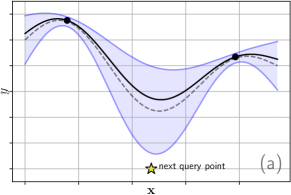
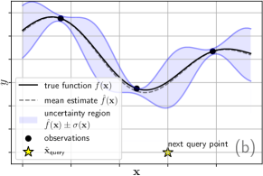
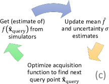
Figure 1: An illustration of the Bayesian optimization process. See Sec 3 for details.

3 ESOP: Epidemiologically and Socio-economically Optimal Policies

ESOP encodes interventions as vectors and their health and socio-economic outcomes as functions, e.g., the coordinates of a 2-D vector ${{\mathbf{x}}}=[{{\mathbf{x}}}_{1},{{\mathbf{x}}}_{2}]\in{\mathbb{N}}^{2}$ may encode the starting point (${{\mathbf{x}}}_{1}$) and duration (${{\mathbf{x}}}_{2}$) of a lock-down. Next, consider a function $f_{\text{epi}}:{\mathbb{N}}^{2}\rightarrow[0,1]$ encoding health outcomes with $f_{\text{epi}}({{\mathbf{x}}})$ equal to the peak infection rate (the largest fraction of the total population infected at any point of time) if the intervention ${{\mathbf{x}}}$ is applied. Similarly, let $f_{\text{eco}}:{\mathbb{N}}^{2}\rightarrow[0,1]$ encode economic outcomes with $f_{\text{eco}}({{\mathbf{x}}})$ being the fraction of population that would face unemployment if lock-down were indeed to last ${{\mathbf{x}}}_{2}$ days. We stress that the functions $f_{\text{epi}},f_{\text{eco}}$ described here are examples and other measurable outcomes, e.g. cumulative death rate, loss to GDP, can also be used. Predicted estimates for $f_{\text{epi}}$ would be obtained from epidemiological simulators such as INDSCI-SIM or IndiaSim (we will use VIPER) and those for $f_{\text{eco}}$ would be obtained from economic models. Our goal is to balance health and economic outcomes by solving the following optimization problem:

$${{\mathbf{x}}}^{\ast}:=\arg\min_{{{\mathbf{x}}}\in{\mathbb{N}}^{2}}\ f({{\mathbf{x}}})\text{ where }f({{\mathbf{x}}})=f_{\text{epi}}({{\mathbf{x}}})+f_{\text{eco}}({{\mathbf{x}}})$$

However, it is challenging to perform this optimization using standard descent techniques (Boyd and Vandenberghe, 2004) since even obtaining values of the function $f$ at specific query points (let alone gradients) is expensive as it involves querying simulators such as VIPER. An acceptable solution in this case is Bayesian optimization (Jones et al., 1998) which is an active machine learning technique used to optimize functions which are expensive to evaluate and to which, moreover we do not have access to gradients.

Fig 1 presents a visual depiction of the key processes in Bayesian optimization. The technique adaptively queries the function at only a few locations to quickly approximate the solution to the optimization problem. The algorithm uses the current observations and Gaussian process regression (Rasmussen and Williams, 2006) to obtain a mean estimate $\hat{f}({{\mathbf{x}}})$ (dashed line in Fig 1) of the true function $f({{\mathbf{x}}})$ (bold line in Fig 1) as well as an estimate $\sigma({{\mathbf{x}}})$ of the uncertainty in that estimate (the blue shaded region depicts $\hat{f}({{\mathbf{x}}})\pm\sigma({{\mathbf{x}}})$ in Fig 1). Notice that uncertainty drops around observation points since (a good estimate of) the true function value is known there.

Using these, an acquisition function is created. Fig 1(a) uses the simple LCB (lower confidence bound) acquisition function defined as $a({{\mathbf{x}}})=\hat{f}({{\mathbf{x}}})-\sigma({{\mathbf{x}}})$. Other possibilities include EI (expected improvement) and KG (knowledge gradient). The (estimated) function value at the point $\hat{{\mathbf{x}}}_{\text{query}}:=\arg\min a({{\mathbf{x}}})$ is now queried. Using $f(\hat{{\mathbf{x}}}_{\text{query}})$, the mean and uncertainty estimates $\hat{f},\sigma$ are updated as shown in Fig 1(b) and the process is repeated. At the end, the query point with the lowest function value is returned as the estimated minimum. Note that ESOP can only query VIPER but does not have access to its internal attribute values.

Lack of space does not permit a detailed overview and we refer the reader to (Frazier, 2018) for an excellent review. ESOP also employs multi-scale search and caching techniques to accelerate computations. Bayesian optimization routines often enjoy provable convergence bounds which we briefly discuss in Sec 4.3.

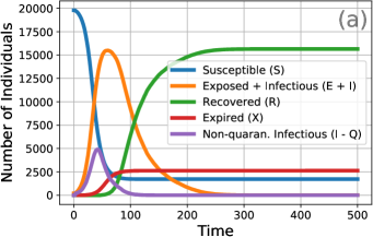
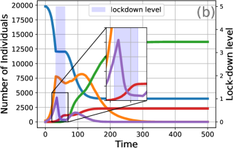
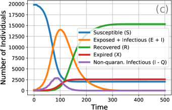
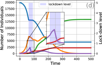
Figure 2: Using ESOP to discover the optimal point at which to initiate a lock-down. Figs 2(a),(b) consider a virus strain with an incubation of 3 days whereas Figs 2(c),(d) consider a strain with a 10 day incubation period. The optimal initiation point of a lock-down depends strongly on viral characteristics e.g. incubation period. ESOP is able to discover a near-optimal initiation point in both cases within very few iterations (see Fig 3. See Sec 4.2 for details.

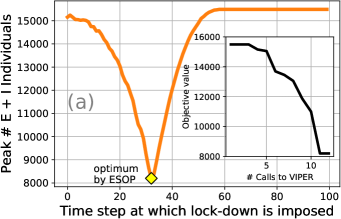
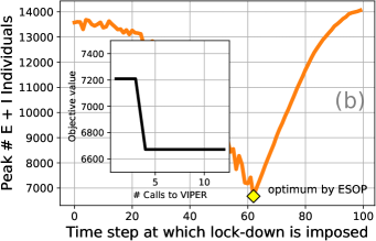
Figure 3: Convergence rates offered by ESOP. Figs 3(a),(b) show (see black curve) ESOP’s convergence rate in the 3 and 10 day incubation period cases in Fig 2. The optimal initiation point varies significantly with the incubation period (33 vs 62 days). See 4.3 for details.

4 Experimental Case Studies

We present case studies with VIPER simulating an in-silico population of 20000 individuals (ESOP scales to larger populations too). The default attributes settings in VIPER are given in Tab 1. Any modifications to these are mentioned below.

4.1 Choice of $f_{\text{epi}}$ and $f_{\text{eco}}$

A lock-down is represented as a 3-D vector ${{\mathbf{x}}}=(i,p,l)$ of its initiation point ($i$), period ($p$) and level ($l$). Our objective is to minimize $f_{\text{epi}}+f_{\text{eco}}$ where $f_{\text{epi}}({{\mathbf{x}}})$ is the peak of the E+I curve. We use $f_{\text{eco}}({{\mathbf{x}}})=\frac{l}{5}\cdot p\cdot\frac{N}{1000}$ to estimate job losses due to the lock-down assuming that a level-$l$ lock-down forces an $\frac{l}{50}$ percent of the population of $N=20000$ into unemployment each day for $p$ days. Note that most natural definitions of $f_{\text{epi}}$ and $f_{\text{eco}}$ would conflict with each other since $f_{\text{epi}}$ would promote aggressive and sustained lock-downs whereas $f_{\text{eco}}$ would oppose them.

The notion of $f_{\text{eco}}(\cdot)$ used above is merely demonstrative and ESOP can instead use a more realistic definition of $f_{\text{eco}}$ that might be a non-linear function of ${{\mathbf{x}}}$, by asking an economic simulator, just as it asks values of $f_{\text{epi}}$ from an epidemiological simulator such as VIPER. Also, defining the objective as an additive sum $f_{\text{epi}}+f_{\text{eco}}$ of the two functions is not necessary essential for ESOP to function and users may instead prefer other formulations e.g. $f_{\text{eco}}^{\alpha}\cdot f_{\text{epi}}^{\beta}$ for some $\alpha,\beta>0$, etc.

All that ESOP requires is black-box access to values of the objective function, however it may be defined. As Fig 3 indicates, ESOP is capable of optimizing highly non-linear functions as well. However, the algorithm would naturally require more iterations if the objective becomes highly convoluted and sensitive to changes in the input (see Sec 5 for a brief discussion).

4.2 Using ESOP to Find the Optimal Initiation Point of a Lock-down

Fig 2 considers a simple case where we have decided to impose a 30 time step lock down at level 5 but are unsure when to initiate the lock down for optimal effect. The objective here is to minimize $f_{\text{epi}}$ alone and $f_{\text{eco}}$ is not considered since we have already decided the duration and intensity of the lock-down in this case and hence resigned to a predictable economic outcome. For any initiation point $i\in{\mathbb{N}}$, let $f_{\text{epi}}(i)$ be the largest number of individuals in E and I states at any given point of time (the so called peak of the curve) if a level 5 lock-down is initiated at $t=i$.

Fig 2(a) shows the daily count of individuals in various categories if no suppression is used. Note the large number of non-quarantined yet infectious individuals (I-Q) who are responsible for disease spread. The number of infected (E+I) individuals peaks at around 15500 at $t=58$. For Fig 2(b), ESOP was asked to suggest when to start a 30 day lock-down at level 5. It suggested starting at $t=33$ which brings the peak down to 8200 cases, a reduction of 47%. Figs 2(c), (d) show similar results but for a viral strain that has an incubation of 10 days instead of 3 days.

The results show that the optimal initiation point depends significantly on disease characteristics, e.g., incubation period of the virus. Nevertheless, ESOP discovers a near-optimal solution, offering far superior health outcomes compared to a no-lock-down scenario. Note that the number of non-quarantined infectious individuals continues to rise (see Fig 2(b), (d) insets) even after imposition of lock-down due to the incubation period of the disease.

4.3 Convergence Rate of ESOP

The topic of how fast do Bayesian optimization routines converge to the optimal solution is a subject of intense study but one beyond the scope of this paper. Under appropriate assumptions, Bayesian optimization routines, within $T$ queries to the underlying function (e.g., as ESOP queries $f_{\text{epi}}$ via VIPER), are able to offer a solution that is only $\epsilon_{T}$ worse than the optimal solution. The sub-optimality $\epsilon_{T}$ goes down with the number of queries $T$ at a rate $\frac{1}{T^{\alpha}}$ where $\alpha>0$ is a constant that depends on the problem setting and the kernel used by the Bayesian optimization procedure (all experiments with ESOP use the Matern kernel). We refer the reader to (Srinivas et al., 2010) for technical details of these convergence results.

Figs 3(a), (b) show that ESOP achieved the globally optimal initiation point for the two cases considered in Fig 2 within just 12 and 4 calls to VIPER (see inset figures). To plot the orange curves in Fig 3, VIPER was queried with all $i\in[0,100]$ to explicitly reveal the globally optimum. This was done so that we could verify that ESOP does indeed reach the global optimum. However, ESOP itself requires far fewer, e.g. 12 or 4 calls to VIPER to reach the global minimum.

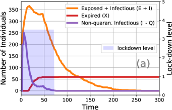
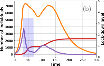
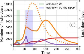
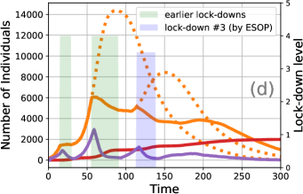
Figure 4: Optimizing (multi-phase) lock-downs under constraints. See Sec 4.4 for details. ESOP is able to shift from a containment strategy (e.g. in Fig 4(a)) to a mitigation strategy (e.g. in Fig 4(b)) depending on the constraints. When multiple spikes are inevitable due to constraints on the lock-down (e.g. upper limits on the duration of the lock-downs), ESOP balances the heights of the spikes to ensure that infections are evenly distributed among them.

4.4 Using ESOP to Optimize (Multi-phase) Lock-downs under Constraints

Administrative and logistical considerations put constraints on lock-downs, e.g., on when a lock-down can be initiated or, on how long it can last. Another constraint might be taking into account previously applied lock-downs. We demonstrate how ESOP can be used to design lock-down schedules that are optimal among those that satisfy a given set of constraints. Fig 4 considers finding the optimal initiation, period and level of a lock-down, subject to constraints.

Single-phase Lock-downs under Constraints.

For Fig 4(a), ESOP was asked to suggest a lock-down (no constraints on duration etc). It suggested one at level 3.5 starting $t=3$, lasting 69 steps, resulting in a peak of 303 infections (much smaller than the peaks in Fig 2) and 1092 predicted cases of unemployment. We note that $f_{\text{eco}}$ prevents the lock-down from going on indefinitely. The suggested lock-down seems to adopt a containment strategy, initiating a moderate-level suppression very early on to deplete the pool of infectious individuals. Note that the pool of non-quarantined infectious individuals is indeed exhausted by the time the suggested lock-down is over, preventing a second wave of infections. For Fig 4(b), ESOP was forced to suggest a lock-down starting no earlier than $t=12$ and lasting no longer than 40 days. Since infections are already rampant by $t=12$, ESOP instead adopts a mitigation strategy of starting a lock-down at $t=30$ for 40 steps at level 3.5, causing a peak of 7353 infections and 560 cases of unemployment. Notice that the lock-down is strategically delayed so that the second wave does not have a higher peak, thus balancing the two peaks indeed as dictated by $f_{\text{epi}}$.

Multi-phase Lock-downs.

For Fig 4(c), ESOP was given a situation where an earlier lock-down (green shading) had already taken place but was ineffective and left alone, would have caused a massive second wave with a peak of 14384 (dotted orange curve). ESOP was asked to suggest a new lock-down that starts no earlier than 10 days after the previous lock-down ended and lasting no longer than 40 days. ESOP suggested a second lock-down starting at $t=56$ lasting 35 steps at level 4 which brings the peak down to 8447 (a reduction of 40%) and causing 560 additional cases of unemployment. Fig 4(d) considers a scenario where the policy makes are still dissatisfied with the outcomes, and request a third lock-down starting no earlier than 10 days after the second lock-down ended and lasting no longer than 40 days. ESOP suggests a third milder lock-down at level 3.5 starting at $t=114$ and lasting 25 days. This brings the peak to a much lower number (6052 i.e. a further 28% reduction) and 350 additional cases of unemployment.

4.5 Can aggressive quarantining permit ESOP to offer less severe lock-downs?

Intuitively, if aggressive quarantining is applied, then it should be possible to avert an epidemic with milder lock-downs. Fig 5 verifies this claim by considering at the situation in Fig 4(b) (i.e. starting a lock-down no earlier than $t=12$ days and lasting no longer than 40 days), but with varying quarantine aggressiveness. As Tab 1 and Sec 2 explain, individuals with viral loads over a threshold QTH get quarantined with a certain probability profile. Using greater screening and public awareness, this profile can be altered.

Fig 5(a) considers sluggish quarantining with QTH = 0.9 and BQP = 0.0 (the quarantining probability profile is shown in Fig 5(a) as an inset). Almost no individuals get quarantined and despite its best efforts, ESOP is only able to offer 11338 peak infections and 800 unemployment cases using a lock-down starting at $t=32$ (level 5, 40 steps). With stronger quarantining at QTH = 0.4 and BQP = 0.3, the situation improves in Fig 5(b) where ESOP offers fewer infections (7930) and job losses (560) using a lock-down at a reduced level of 3.5 (starting $t=30$, 40 steps). With still stronger quarantining (QTH = 0.0, BQP = 0.0) in Fig 5(c), ESOP offers a peak of 871 and 378 job losses using a lock-down lasting fewer (27) steps (starting $t=15$, level 3.5). Fig 5(c) reports the outcomes with even stronger quarantining at QTH = 0.2 and BQP = 0.5 where ESOP offers a peak of just 706 and 192 job losses using a lock-down lasting just 16 steps(level 3 starting $t=12$).

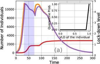
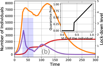
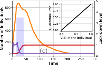
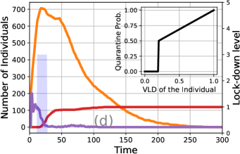
Figure 5: Effect of quarantine policy on ESOP’s ability to offer desirable outcomes. The area under the black curve in the insets roughly measures the aggressiveness of the quarantining policy. See Sec 4.5 for details. ESOP offers better outcomes, both epidemiologically as well as economically, and that too with milder lock-downs, if strong quarantining is applied.

4.6 Variations in Demographics and Geographical Distribution of Population

We also consider location (X, Y), susceptibility (SUS) and resistance (RST) values (see Tab 1) which are not set uniformly but fitted to statistical data for India.

Population Clusters. Instead of distributing individuals uniformly in the box $[0,1]^{2}$, as we did earlier, we now distribute 34% of the population into 4 Gaussian clusters with standard deviation 0.1 (to simulate crowded urban areas). India does have a similar proportion of urban population (Bank, 2018). We distribute the rest 66% of the population uniformly (to simulate scattered non-urban population).

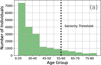
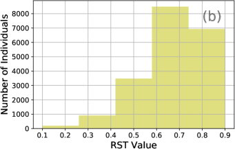
Figure 6: Demographic data fitted to Indian statistics. The demographic advantage of the Indian population is evident from both curves. Fig 6(a) shows that the vast majority of the population do not cross the risk-factor forming seniority threshold whereas Fig 6(b) shows that most individuals have high RST value i.e. resistance to infection, as calculated in Sec 4.6.

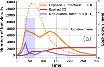
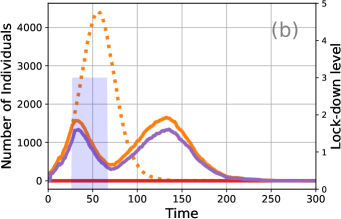
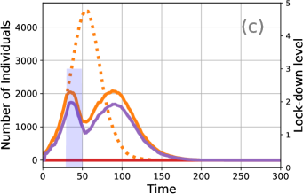
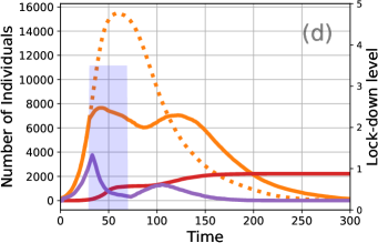
Figure 7: ESOP with fitted demographic and location data. See Sec 4.6.1 for details. The dotted lines in all figures gives the infection curve had no lock-down been applied.

Fitted Demographic Data. Instead of distributing SUS and RST values uniformly in $[0,1]$ as we did earlier, we now distribute these according to age and co-morbidity statistics for India. (Joshi, 2020, Table 1) reports that the four factors with highest risk score for CoViD-19 patients are age above 55 years, male gender, hypertension, and diabetes. We collected age-stratified statistics for all these factors from respectively (Home Affairs India, 2016, Detailed Tables), (Ramakrishnan et al., 2019, Table 1) and (Group, 2003, Table 2). After assigning age, gender, and co-morbidity values to alll individuals so as to fit the Indian statistics, individuals were assigned a point each for being male, over 55, and suffering from each of the two co-morbidities. Thus, an individual could clock up a maximum of 4 points. An individual’s SUS value was then decided as $0.1+0.2\times\text{ \#points }$. Their RST value was set to $\text{RST}=1-\text{SUS}$. Fig 6(b) shows the resulting distributions.

4.6.1 Results with Fitted Demographic Data and Population Clusters

Fig 7(a) is identical to Fig 4(b) (where ESOP was asked for a lock-down lasting no longer than 40 days and starting no earlier than $t=12$) except that Fig 7(a) also shows (using a dotted orange line) what the infection curve would have been, had no lock-down been applied at all. Recall that with the lock-down suggested by ESOP, we had a peak of 7353 infections and 560 cases of unemployment. Fig 7(b) presents the situation where we use population clusters as well as fitted demographic data. The improvement with ESOP’s new suggestion is extremely significant with a peak of just 1653 infections (more than $4\times$ reduction) and 480 cases of unemployment, that too, using a milder lock-down at level 3.0.

To ascertain whether this improvement was due to the demographic change or the population clusters, Figs 7(c),(d) present ablation studies. In Fig 7(c), only the demographic distributions of RST and SUS are fitted to Indian data but locations are kept uniformly distributed over the 2-D box $[0,1]^{2}$ as we were doing earlier. In Fig 7(d), RST and SUS values are uniformly distributed over $[0,1]$ as we were doing earlier, but 34% of the population is clustered into “cities”.

It is clear that changing the location distribution of the individuals alone worsens the outcome (Fig 7(d) reports a peak of 7657 that is higher than Fig 7(a)). This is to be expected since people are now crowded into cities . However, changing the demographics of the population to match that of India greatly improves the outcome (Fig 7(c) reports a peak of just 2083 and just 240 cases of unemployment). This is also to be expected since India has an extremely favorable age structure. Since applying both changes together, as in Fig 7(b), also presents a significant improvement over Fig 7(a), this seems to suggest that the demographic advantages more than overcome the disadvantage due to crowding in cities.

5 Concluding Remarks

Incorporating age stratification and climate into VIPER and augmenting ESOP to suggest “personalized” age- and climate-specific policies would be interesting. It would also be interesting to develop epidemiological models that simultaneously track multiple diseases with similar or confounding symptoms, such as CoViD-19 and ILI (Influenza-like illnesses) as it would allow policy models e.g. testing and quarantining models to be checked for false positive and missed detection rates. Lastly, non-linear systems with negative feedback loops such as epidemiological models, are known to exhibit chaotic behavior (Bolker, 1993; Eilersen et al., 2020). It is interesting how techniques like ESOP can be adapted to handle such systems.

5.1 Relevance to CoViD-19 and Future Prospects

Given the evolving nature of the current CoViD-19 pandemic, a technique like ESOP helps in optimally designing multi-phase lock-downs, thus avoiding speculation and human error. As shown in Sec 4, whenever multiple waves of infection are unavoidable due to constraints on lock-downs, ESOP offers lock-down schedules that balance the peaks of these multiple outbreaks, ensuring no peak is too high. To maximize the impact of methods such as ESOP, close interaction and collaboration is needed with experts in the epidemiological and social sciences to better align ESOP with professional epidemiological forecasting and economic forecasting models. ESOP’s interaction with these models is of a black-box nature which makes integration smoother and simpler.

Conflict of Interest

The authors declare that they have no conflict of interest.

Code Availability

All code used for this study is available at the following GitHub Repository
https://github.com/purushottamkar/esop

References

- Aledort et al. [2007] Julia E Aledort, Nicole Lurie, Jeffrey Wasserman, and Samuel A Bozzette. Non-pharmaceutical public health interventions for pandemic influenza: an evaluation of the evidence base. BMC Public Health, 7(208), 2007.
- Bank [2018] The World Bank. Urban population (% of total population) - India. https://data.worldbank.org/indicator/SP.URB.TOTL.IN.ZS?locations=IN, 2018.
- Bolker [1993] Benjamin Bolker. Chaos and complexity in measles models: A comparative numerical study. IMA Journal of Mathematics Applied in Medicine & Biology, 10:83–95, 1993.
- Boyd and Vandenberghe [2004] Stephen Boyd and Lieven Vandenberghe. Convex Optimization. Cambridge University Press, 2004.
- Bussell et al. [2019] E. H. Bussell, C. E. Dangerfield, C. A. Gilligan, and N. J. Cunniffe. Applying optimal control theory to complex epidemiological models to inform real-world disease management. Philosophical Transactions of the Royal Society B, 374(1776), 2019.
- Dandekar and Barbastathis [2020] Raj Dandekar and George Barbastathis. Neural Network aided quarantine control model estimation of global Covid-19 spread. arXiv:2004.02752v1 [q-bio.PE], April 2020.
- Efimov and Ushirobira [2020] Denis Efimov and Rosane Ushirobira. On an interval prediction of COVID-19 development based on a SEIR epidemic model. Technical report, Inria Lille Nord Europe - Laboratoire CRIStAL - Université de Lille, April 2020. hal-02517866v4.
- Eilersen et al. [2020] Andreas Eilersen, Mogens H. Jensen, and Kim Sneppen. Chaos in disease outbreaks among prey. Scientific Reports, 10(3907), 2020.
- Ferguson et al. [2020] Neil M Ferguson, Daniel Laydon, Gemma Nedjati-Gilani, Natsuko Imai, Kylie Ainslie, Marc Baguelin, Sangeeta Bhatia, Adhiratha Boonyasiri, Zulma Cucunubá, Gina Cuomo-Dannenburg, Amy Dighe, Ilaria Dorigatti, Han Fu, Katy Gaythorpe, Will Green, Arran Hamlet, Wes Hinsley, Lucy C Okell, Sabine van Elsland, Hayley Thompson, Robert Verity, Erik Volz, Haowei Wang, Yuanrong Wang, Patrick GT Walker, Caroline Walters, Peter Winskill, Charles Whittaker, Christl A Donnelly, Steven Riley, and Azra C Ghani. Impact of non-pharmaceutical interventions (NPIs) to reduce COVID-19 mortality and healthcare demand. Technical report, Imperial College London, 2020.
- Frazier [2018] Peter I. Frazier. A Tutorial on Bayesian Optimization. arXiv:1807.02811v1 [stat.ML], July 2018.
- Group [2003] The DECODA Study Group. Age- and Sex-Specific Prevalence of Diabetes and Impaired Glucose Regulation in 11 Asian Cohorts. Diabetes Care, 26(6):1770–1780, 2003.
- Harsha et al. [2020] Prahladh Harsha, Sandeep Juneja, Preetam Patil, Nihesh Rathod, Ramprasad Saptharishi, A. Y. Sarath, Sharad Sriram, Piyush Srivastava, Rajesh Sundaresan, and Nidhin Koshy Vaidhiyan. COVID-19 Epidemic Study II: Phased Emergence From the Lockdown in Mumbai. arXiv:2006.03375 [q-bio.PE], 2020.
- Home Affairs India [2016] Office of Ministry Home Affairs India. Sample Registration System Statistical Report 2016. https://censusindia.gov.in/vital_statistics/SRS_Reports__2016.html, 2016. Accessed 14 June, 2020.
- Jones et al. [1998] Donald R. Jones, Matthias Schonlau, and William J. Welch. Efficient Global Optimization of Expensive Black-Box Functions. Journal of Global Optimization, 13:455–492, 1998.
- Joshi [2020] Shashank R Joshi. Indian COVID-19 Risk Score, Comorbidities and Mortality. Journal of The Association of Physicians of India, 68(5):11–12, 2020.
- Keeling and Rohani [2008] Matt J. Keeling and Pejman Rohani. Modeling Infectious Diseases in Humans and Animals. Princeton University Press, 2008.
- Kimball and Bose [2020] Ryder Kimball and Debanjali Bose. 11 pandemics that changed the course of human history, from the Black Death to HIV/AIDS - to coronavirus. Business Insider India, March 2020. https://www.businessinsider.in/science/news/11-pandemics-that-changed-the-course-of-human-history-from-the-black-death-to-hiv/aids-to-coronavirus/articleshow/74695609.cms. Accessed 19 April 2020.
- Klepac et al. [2011] Petra Klepac, Ramanan Laxminarayan, and Bryan T. Grenfell. Synthesizing epidemiological and economic optima forcontrol of immunizing infections. Proceedings of the National Academy of Sciences, 108(34):14366–14370, 2011.
- Lindström et al. [2015] Tom Lindström, Michael Tildesley, and Colleen Webb. A Bayesian Ensemble Approach for Epidemiological Projections. PLOS Computational Biology, 11(4):e1004187, 2015.
- Lyra et al. [2020] Wladimir Lyra, José-Dias do Nascimento Jr., Jaber Belkhiria, Leandro de Almeida, Pedro Paulo M. Chrispim, and Ion de Andrade. COVID-19 pandemics modeling with SEIR(+CAQH), social distancing, and age stratification. The effect of vertical confinement and release in Brazil. medRxiv: 2020.04.09.20060053, April 2020.
- Megiddo et al. [2014] Itamar Megiddo, Abigail R. Colson, Arindam Nandi, Susmita Chatterjee, Shankar Prinja, Ajay Khera, and Ramanan Laxminarayan. Analysis of the Universal Immunization Programme and introduction of a rotavirus vaccine in India with IndiaSim. Vaccine, 325:A151–A161, 2014.
- Morris et al. [2020] Dylan H. Morris, Fernando W. Rossine, Joshua B. Plotkin, and Simon A. Levin. Optimal, near-optimal, and robust epidemic control. arXiv:2004.02209v1 [q-bio.PE], April 2020.
- Nagori et al. [2020] Aditya Nagori, Raghav Awasthi, Vineet Joshi, Suryatej Reddy Vyalla, Akhil Jarodia, Chandan Gupta, Amogh Gulati, Harsh Bandhey, Ponnurangam Kumaraguru, and Tavpritesh Sethi. Less Wrong COVID-19 Projections With Interactive Assumptions. medRxiv: 2020.06.06.20124495, 2020.
- Patterson-Lomba [2020] Oscar Patterson-Lomba. Optimal timing for social distancing during an epidemic. medRxiv: 2020.03.30.20048132, April 2020.
- Peak et al. [2017] Corey M. Peak, Lauren M. Childs, Yonatan H. Grad, and Caroline O. Buckee. Comparing nonpharmaceutical interventions forcontaining emerging epidemics. Proceedings of the Nat. Acad. Sci. USA Sciences of the USA, 114(15):4023–4028, 2017.
- Perrings et al. [2014] Charles Perrings, Carlos Castillo-Chavez, Gerardo Chowell, Peter Daszak, Eli P. Fenichel, David Finnoff, Richard D. Horan, A. Marm Kilpatrick, Ann P. Kinzig, Nicolai V. Kuminoff, Simon Levin, Benjamin Morin, Katherine F. Smith, and Michael Springborn. Merging Economics and Epidemiology to Improve thePrediction and Management of Infectious Disease. Ecohealth, 11(4):464–475, 2014.
- Ramakrishnan et al. [2019] Sivasubramanian Ramakrishnan et al. Prevalence of hypertension among Indian adults: Results from the great India blood pressure survey. Indian Heart Journal, 71(4):309–313, 2019.
- Rasmussen and Williams [2006] Carl Edward Rasmussen and Christopher K. I. Williams. Gaussian Processes for Machine Learning. MIT Press, 2006.
- Roos [2012] Robert Roos. CDC estimate of global H1N1 pandemic deaths: 284,000. Newsletter of the Center for Infectious Disease Research and Policy, University of Minnesota, June 2012. https://www.cidrap.umn.edu/news-perspective/2012/06/cdc-estimate-global-h1n1-pandemic-deaths-284000. Accessed 19 April 2020.
- Sardar et al. [2020] Tridip Sardar, Sk Shahid Nadimb, and Joydev Chattopadhyay. Assessment of 21 Days Lockdown Effect in Some States and Overall India: A Predictive Mathematical Study on COVID-19 Outbreak. arXiv:2004.03487v1 [q-bio.PE], April 2020.
- Scherbina [2020] Anna Scherbina. Determining the Optimal Duration of the COVID-19 Suppression Policy https://dx.doi.org/10.2139/ssrn.3562053. Accessed 19 April 2020., March 2020.
- Shekatkar et al. [2020] Snehal Shekatkar, Bhalchandra Pujari, Mihir Arjunwadkar, Dhiraj Kumar Hazra, Pinaki Chaudhuri, Sitabhra Sinha, Gautam I Menon, Anupama Sharma, and Vishwesha Guttal. INDSCI-SIM: A state-level epidemiological model for India, 2020. Ongoing Study at https://indscicov.in/indscisim.
- Singh and Adhikari [2020] Rajesh Singh and Ronojoy Adhikari. Age-structured impact of social distancing on the COVID-19 epidemic in India. arXiv:2003.12055v1 [q-bio.PE], March 2020.
- Srinivas et al. [2010] Niranjan Srinivas, Andreas Krause, Sham Kakade, and Matthias Seeger. Gaussian Process Optimization in the Bandit Setting: No Regret and Experimental Design. In Proceedings of the 27th International Conference on Machine Learning (ICML), 2010.
- Torre et al. [2019] Davide La Torre, Tufail Malik, and Simone Marsiglio. Optimal Control of Prevention and Treatment in a Basic Macroeconomic-Epidemiological Model. arXiv:1910.03383 [econ.TH], 2019.
- Vyasarayani and Chatterjee [2020] C. P. Vyasarayani and Anindya Chatterjee. New approximations, and policy implications, from a delayed dynamic model of a fast pandemic. arXiv:2004.03487v1 [q-bio.PE], April 2020.
- Wallinga et al. [2010] Jacco Wallinga, Michiel van Boven, and Marc Lipsitch. Optimizing infectious disease interventions during an emerging epidemic. Proceedings of the Nat. Acad. Sci. USA Sciences of the USA, 107(2):923–928, 2010.
- WHO [2020] WHO. Coronavirus disease (COVID-19) Pandemic, April 2020. https://www.who.int/emergencies/diseases/novel-coronavirus-2019. Accessed 07 June 2020.
- Zhao and Feng [2019] Henry Zhao and Zhilan Feng. Identifying Optimal Vaccination Strategies via Economic and Epidemiological Modeling. Journal of Biological Systems, 27(4):423–446, 2019.