[sakumoto@kwansei.ac.jp]Yusuke Sakumotomkwansei [ohsaki@kwansei.ac.jp]Hiroyuki Ohsakimkwansei

[kwansei]Kwansei Gakuin University, 2-1 Gakuen, Sanda, Hyogo 669-1337, Japan

Graph Degree Heterogeneity Facilitates Random Walker Meetings

Various graph algorithms have been developed with multiple random walks, the movement of several independent random walkers on a graph. Designing an efficient graph algorithm based on multiple random walks requires investigating multiple random walks theoretically to attain a deep understanding of their characteristics. The first meeting time is one of the important metrics for multiple random walks. The first meeting time on a graph is defined by the time it takes for multiple random walkers to meet at the same node in a graph. This time is closely related to the rendezvous problem, a fundamental problem in computer science. The first meeting time of multiple random walks has been analyzed previously, but many of these analyses have focused on regular graphs. In this paper, we analyze the first meeting time of multiple random walks in arbitrary graphs and clarify the effects of graph structures on expected values. First, we derive the spectral formula of the expected first meeting time on the basis of spectral graph theory. Then, we examine the principal component of the expected first meeting time using the derived spectral formula. The clarified principal component reveals that (a) the expected first meeting time is almost dominated by $n/(1+d_{\rm std}^{2}/d_{\rm avg}^{2})$ and (b) the expected first meeting time is independent of the starting nodes of random walkers, where $n$ is the number of nodes of the graph. $d_{\rm avg}$ and $d_{\rm std}$ are the average and the standard deviation of weighted node degrees, respectively. The characteristic (a) is useful for understanding the effect of the graph structure on the first meeting time. According to the revealed effect of graph structures, the variance of the coefficient $d_{\rm std}/d_{\rm avg}$ (degree heterogeneity) for weighted degrees facilitates the meeting of random walkers.

1 Introduction

Various graph algorithms have been developed with multiple random walks, the movement of several independent random walkers on a graph, as a result of graph algorithms’ ease of analysis and light-weight processing. Notable applications include (a) a search algorithm for finding a particular node on a graph [1, 2], (b) an algorithm for spreading information across graphs by exchanging information only between adjacent nodes [3], and (c) the rendezvous algorithm for efficient meeting of multiple random walkers at the same node [4]. Designing an efficient graph algorithm based on multiple random walks requires studying multiple random walks theoretically in order to understand their characteristics at a deep level.

Several important metrics (e.g., first hitting time, recurrence time, cover time, re-encountering time, and first meeting time) have been used for multiple random walks. The first hitting time is the time it takes for any random walker to arrive at a specified node, and it is important for evaluating the performance of relevant search algorithms. The recurrence time is the time required to return any one of the random walkers to the starting node, and it is thus a particular case of the first hitting time. The cover time is the time it takes for any random walker to reach all of the nodes and corresponds to the maximum value of the first hitting times. The cover time strongly affects the information dissemination speed in the graph. The re-encountering time and the first meeting time are the times it takes for multiple random walkers to meet at the same node. The re-encountering time relates to random walkers starting from the same node, and the first meeting time relates to those starting from different nodes. In particular, the first meeting time is closely related to the rendezvous problem, a fundamental problem in computer science. The rendezvous problem occurs in a number of engineering problems (e.g., the self-stabilizing token management system problem [5, 6] and the $k$-server problem [7]). Designing efficient algorithms for the rendezvous problem requires clarification of the characteristics of the first meeting time.

The first meeting time of multiple random walks was analyzed in [8, 9, 10, 11, 12]. However, many of these previous studies focus on regular graphs. In [12], George et al. did pioneering work on multiple random walks on non-regular graphs and derived a closed-form formula for calculating the expected value of the first meeting time in arbitrary graphs. However, the effects of graph structures on the expected first meeting time remain unclear. Designing effective algorithms using multiple random walks for realistic graphs (e.g., social networks and communication networks) benefits from understanding the effects of graph structures on the expected first meeting time. Since it is difficult to clarify these effects numerically using the closed-form formula derived in [12], the effects must be examined using analysis of multiple random walks.

In this paper, we analyze the first meeting time of multiple random walks in arbitrary graphs and clarify the effects of graph structures on its expected value. First, we derive the spectral formula of the expected first meeting time on the basis of spectral graph theory that is used to analyze the characteristics of graphs. Then, we examine the principal component of the expected first meeting time using the derived spectral formula. The clarified principal component reveals that (a) the expected first meeting time is almost dominated by $n/(1+d_{\rm std}^{2}/d_{\rm avg}^{2})$, where $n$ is the number of nodes in the graph and $d_{\rm avg}$ and $d_{\rm std}$ are the average and standard deviation of weighted node degrees, respectively, and (b) the expected first meeting time is independent of the starting nodes of random walkers. Characteristic (a) provides understanding of the effect of the graph structure on the first meeting time. In addition, we verify the validity of the analysis results through numerical examples.

The contributions in this paper are summarized as follows.

• We extend the analysis of a single random walks to multiple random walks using spectral graph theory.

• We derive the spectral formula of the expected first meeting time.

• We clarify the principal component of the expected first meeting time.

• We reveal the effect of graph structures on the expected first meeting time.

• We confirm the validity of the derived spectral formula and the clarified principal component for various networks with different scales and different structures.

The remainder of this paper is organized as follows. In Sect. 2, we describe the definition of graphs and random walks and introduce the previous analysis of a single random walk using spectral graph theory. In Sect. 3, we derive the spectral formula of the expected first meeting time using spectral graph theory and clarify the principal component of the expected first meeting time on the basis of the derived spectral formula. Sect. 4 confirms the validity of the analysis results through numerical examples. Sect. 5 concludes the paper and discusses future work.

2 Preliminary

In this section, we provide the definition of graphs and random walks that we use in our analysis. In addition, we review existing analysis results of a single random walk based on spectral graph theory.

A graph is given by $G=(V,E)$, where $V$ and $E$ are a set of nodes and a set of links, respectively. Self-loop links $(i,i)$ for $i\in V$ are not included in $E$. The weight for link $(i,j)\in E$ is $w_{ij}$, where $w_{ij}>0$ and $w_{ij}=w_{ji}$. We denote the set of adjacent nodes of node $i\in V$ by $\partial i$. Letting $d_{i}$ be the weighted degree of node $i\in V$, we define $d_{i}$ as

$$d_{i}:=\sum_{k\in\partial i}w_{ik}.$$ (1)

We describe a random walk starting from node $a\in V$. In this random walk, the random walker at node $i\in V$ moves to adjacent node $j\in\partial i$ using transition probability $p_{i\rightarrow j}$ given by

$$p_{i\rightarrow j}=\frac{w_{ij}}{d_{i}}.$$ (2)

Let $x_{a:i}(t)$ be the probability that a random walker starting from node $a\in V$ is at node $i\in V$ at time $t$, where $\sum_{i\in V}x_{a:i}(t)=1$. If Eq. (2) is used, then $x_{a:i}(t+1)$ is

$$x_{a:i}(t+1) =\sum_{j\in\partial i}x_{a:j}(t)\,p_{j\rightarrow i}.$$ (3)

Using column vector $\bm{x}_{a}(t)=(x_{a:i}(t))_{i\in V}$, Eq. (3) for all nodes $\forall i\in V$ can be written simultaneously as

$$\bm{x}_{a}(t+1) =\bm{A}\,\bm{D}^{-1}\,\bm{x}_{a}(t),$$ (4)

where $\bm{D}$ and $\bm{A}$ are the degree and adjacency matrices defined as

$$\bm{D} :={\rm diag}(d_{i})_{i\in V},$$ (5)

$$\bm{A} :=\left\{\begin{array}[]{ll}w_{ij}&\mathrm{if}\ \ (i,j)\in E\\ 0&\mathrm{otherwise}\end{array}\right.,$$ (8)

respectively. $\bm{A}\,\bm{D}^{-1}$ is the matrix whose $(i,j)$th element is the transition probability $p_{j\rightarrow i}$. Equation (4) describes the behavior of the random walk. Since $\bm{A}\,\bm{D}^{-1}$ is an asymmetric matrix, Eq. (4) is not easy to handle analytically using linear algebra. Consequently, we modify Eq. (4) to

$$\bm{D}^{-1/2}\,\bm{x}_{a}(t+1) =\bm{D}^{-1/2}\,\bm{A}\,\bm{D}^{-1/2}\,\bm{D}^{-1/2}\,\bm{x}_{a}(t)$$

$$=\bm{W}\,\bm{D}^{-1/2}\,\bm{x}_{a}(t)$$

$$\bm{\hat{x}}_{a}(t+1) =\bm{W}\,\bm{\hat{x}}_{a}(t),$$ (9)

where $\bm{W}=\bm{D}^{-1/2}\,\bm{A}\,\bm{D}^{-1/2}$ and $\bm{\hat{x}_{a}}(t)=\bm{D}^{-1/2}\,\bm{x}_{a}(t)$. Since $\bm{W}$ is a symmetric matrix, Eq. (9) is easier to handle than Eq. (4). In general, in spectral graph theory, the behavior of an analysis target is expressed in terms of a matrix such as Eq. (9), and the characteristics of the target are analyzed using the eigenvalues and eigenvectors of the matrix on the basis of linear algebra.

$\bm{W}$ can always be diagonalized using the orthogonal matrix $\bm{Q}$ that satisfies ${}^{t}\bm{Q}=\bm{Q}^{-1}$. Let $\lambda_{k}$ be the $k$th largest eigenvalue of $\bm{W}$. Note that the maximum eigenvalue $\lambda_{1}$ is always $1$. In this paper, we assume that $G$ is connected and not a bipartite graph. In this case, the eigenvalues $\lambda_{k}$ for $2\leq k\leq n$ satisfy

$$-1<\lambda_{n}<\cdots<\lambda_{2}<1.$$ (10)

We let $\bm{q}_{k}$ be the eigenvector for eigenvalue $\lambda_{k}$ by, with the consequence that $\bm{Q}$ is $\bm{Q}=(\bm{q}_{k})_{1\leq k\leq n}$. Since $\bm{Q}$ is an orthogonal matrix, $\bm{q}_{k}$ and $\bm{q}_{l}$ for $1\leq k,l\leq n$ satisfy

$${}^{t}\bm{q}_{k}\,\bm{q}_{l}=\left\{\begin{array}[]{ll}1&\mathrm{if}\ \ k=l\\ 0&\mathrm{oterwise}\end{array}\right.$$ (13)

In particular, the maximum eigenvector $\bm{q}_{1}$ is

$$\bm{q}_{1}=\frac{1}{\sqrt{s_{1}}}{}^{t}(\sqrt{d_{1}},\sqrt{d_{2}},\cdots,\sqrt{d_{n}}),$$ (14)

where $s_{1}=\sum_{i\in V}d_{i}$. $s_{1}$ is related to a statistic of the graph structure of $G$ and can be written by $s_{1}=n\,d_{\rm avg}$, where $d_{\rm avg}$ is the average weighted degree.

In [13], Lovász analyzed a single random walk on graph $G$ on the basis of spectral graph theory. Solving Eq. (9) in [13] results in the probability $x_{a:i}(t)$ being

$$x_{a:i}(t) =\frac{\sqrt{d_{i}}}{\sqrt{d_{a}}}\sum_{k=1}^{n}q_{k}(a)\,q_{k}(i)\,\lambda_{k}^{t}.$$ (15)

According to this equation, $x_{a:i}(t)$ can be calculated using eigenvalues $\lambda_{k}$ and eigenvectors $\bm{q}_{k}$. A closed-form formula using eigenvalues and eigenvectors such as Eq. (15) is referred to as a spectral formula.

Let $x_{a:i}^{*}$ be the limit value of $x_{a:i}(t)$ for $t\rightarrow\infty$. From Eq. (15), $x_{a:i}^{*}$ can be derived as

$$x_{a:i}^{*} =\lim_{t\rightarrow\infty}x_{a:i}(t)$$

$$=\lim_{t\rightarrow\infty}\left[\frac{\sqrt{d_{i}}}{\sqrt{d_{a}}}q_{1}(i)\,q_{1}(s)+\frac{\sqrt{d_{i}}}{\sqrt{d_{a}}}\sum_{k=2}^{n}q_{k}(a)\,q_{k}(i)\,\lambda_{k}^{t}\right]$$

$$=\frac{\sqrt{d_{i}}}{\sqrt{d_{a}}}q_{1}(a)\,q_{1}(i)=\frac{d_{i}}{s_{1}}.$$ (16)

In this derivation process, we used $|\lambda_{k}|<1$ for $k\geq 2$. According to Eq. (16), $x_{a:i}(t)$ is roughly proportional to the weighted degree $d_{i}$ if sufficient time has elapsed since the random walker started.

The analysis in [13] derived the expected first hitting time $\mu_{a:i}$, the expected time it takes for a random walker starting from node $a$ to arrive at node $i$. From Eq. (15), the spectral formula of expected first hitting time $\mu_{a:i}$ is derived as

$$\mu_{a:i} =s_{1}\sum_{k=2}^{n}\frac{1}{1-\lambda_{k}}\left(\frac{q_{k}^{2}(i)}{d_{i}}-\frac{q_{k}(a)\,q_{k}(i)}{\sqrt{d_{a}\,d_{i}}}\right).$$ (17)

In [14], the effect of the graph structure on $\mu_{a:i}$ was clarified using the spectral formula of the expected first hitting time $\mu_{a:i}$. According to [14], $\mu_{a:i}$ satisfies

$$\left|\frac{1}{s_{1}}\mu_{a:i}-\frac{1}{d_{i}}\right|\leq\frac{2\,w_{\mathrm{max}}}{d^{2}_{\mathrm{min}}}\left(\frac{1}{1-\lambda_{2}}+1\right),$$ (18)

where $w_{\mathrm{max}}$ and $d_{\mathrm{min}}$ are the maximum of link weights and the minimum of weighted degrees, respectively. If the right-hand side of Eq. (18) is sufficiently small, the expected first hitting time $\mu_{a:i}$ is approximated by

$$\mu_{a:i}\approx\frac{s_{1}}{d_{i}}.$$ (19)

In this case, $\mu_{a:i}$ is almost dominated by $s_{1}/d_{i}$, with the consequence that $s_{1}/d_{i}$ can be expected to be the principal component of $\mu_{a:i}$. According to Eq. (19), $\mu_{a:i}$ is roughly proportional to $s_{1}$, which is a statistic of the graph structure. In other words, $\mu_{a:i}$ corresponds to the search time of node $i$ using the random walk. Therefore, Eq. (19) is also important for understanding the characteristics of the search algorithm using a random walk.

3 Analysis

In this section, we analyze the expected first meeting time $\mu_{a,b}$ of two random walkers starting from node $a\in V$ and $b\in V$ in graph $G$ on the basis of spectral graph theory. We first derive the spectral formula of $\mu_{a,b}$. Then, we clarify the principal component of $\mu_{a,b}$ using the derived spectral formula. Finally, we reveal the effect of the graph structure on $\mu_{a,b}$ on the basis of the clarified principal component.

Our analysis results are important also for understanding the first meeting time of $n_{\rm RW}$ random walkers, where $n_{\rm RW}>2$, because it is strongly affected by the first meeting time of two random walkers. To attain an efficient meeting of $n_{\rm RW}$ random walkers, two of the $n_{\rm RW}$ random walkers must move together after meeting at the same node. In this case, the first meeting time of $n_{\rm RW}$ random walkers is obtained as the sum of the first meeting times of two random walkers. Consequently, the characteristics of the first meeting time for $n_{\rm RW}$ random walkers can be expected to be strongly associated with that of two random walkers.

3. 1 Spectral Formula of Expected First Meeting Time $\mu_{a,b}$

We derive the spectral formula of the expected first meeting time $\mu_{a,b}$ using the same method as is used to derive that of the expected first hitting time $\mu_{a:i}$ in [13]. In [13], the spectral formula was derived using the generating function of the existing probability $x_{a:i}(t)$. In general, the generating function $F(z)$ of the probability $f(t)$ is

$$F(z):=\sum_{t=0}^{\infty}f(t)z^{t}.$$ (20)

Using the generating function $F(z)$, the expectation ${\rm E}(t)$ with the probability $f(t)$ is

$${\rm E}(t)=\sum_{t=1}^{\infty}t\,f(t)=\left.\frac{{\rm d}F(z)}{{\rm d}z}\right|_{z=1}.$$ (21)

Importantly, even if we do not know the clused-form formula of the probability $f(t)$, we can still derive the expectation ${\rm E}(t)$ using the generating function $F(z)$ on the basis of the above equation. We first obtain the generating function of the first meeting probability. Without the value of the first meeting probability, we then derive the spectral formula of the expected first meeting time $\mu_{a,b}$ by substituting the generating function obtained into Eq. (21).

Let $r_{a,b:c}(t)$ be the probability that two random walkers first meet at node $c$ at time $t$. Since two random walkers can meet at any node, the first meeting probability $r_{a,b:*}(t)$ is

$$r_{a,b:*}(t)=\sum_{c\in V}r_{a,b:c}(t).$$ (22)

In $r_{a,b:*}(t)$, the symbol $*$ designates any node in $V$. Deriving the spectral formula of the expected first meeting time $\mu_{a,b}$ using Eq. (21) requires the generating function $R_{a,b:*}(z)$ of $r_{a,b:*}(t)$.

The probabilities that the two random walkers are at node $i$ at time $t$ are $x_{a:i}(t)$ and $x_{b:i}(t)$, respectively. Since the spectral formulas of $x_{a:i}(t)$ and $x_{b:i}(t)$ are given by Eq. (15), the generating functions of $x_{a:i}(t)$ and $x_{b:i}(t)$ can be derived using Eq. (20). However, since it is not easy to obtain the spectral formula of $r_{a,b:*}(t)$, we obtain the generating function $R_{a,b:*}(z)$ of $r_{a,b:*}(t)$ from those of $x_{a:i}(t)$ and $x_{b:i}(t)$ and then derive the spectral formula of the expected first meeting time $\mu_{a,b}$ using Eq. (21).

With the aim of obtaining the generating function $R_{a,b:*}(z)$ of the first meeting probability $r_{a,b:*}(t)$, we discuss the relationship between $r_{a,b:*}(t)$, $x_{a:i}(t)$ and $x_{b:i}(t)$. Let $x_{a,b:c}(t)$ be the probability that the two random walker meet at the same node $c\in V$ at time $t$. The meeting probability $x_{a,b:*}(t)$ at any node is

$$x_{a,b:*}(t)=\sum_{c\in V}x_{a,b:c}(t).$$ (23)

Since each random walker moves independently, $x_{a,b:*}(t)$ is

$$x_{a,b:*}(t)=\sum_{c\in V}x_{a,b:c}(t)=\sum_{c\in V}x_{a:c}(t)\,x_{b:c}(t).$$ (24)

$x_{a,b:*}(t)$ includes both the first meeting probability $r_{a,b:*}(t)$ and also the probability of the second and subsequent meetings. Hence, as shown in Fig. 1, we divide the transition of the two random walks from time $0$ to time $t$ into two transitions, (a) the transition until they first meet at time $s$, and (b) the rest transition. The probability for the former transition is the first meeting probability $r_{a,b:*}(t)$. The probability for the latter transition is the probability that the two random walkers starting from same node $c^{\prime}\in V$ at time $s$ meet again at the same node $c\in V$ at time $t$. Since node $c^{\prime}$ and node $c$ can be any node, we denote such a probability by $x_{*^{\prime},*^{\prime}:*}(t-s)$. With these probabilities, $x_{a,b:*}(t)$ is

$$x_{a,b:*}(t)=\sum_{s=0}^{t}r_{a,b:*^{\prime}}(s)\,x_{*^{\prime},*^{\prime}:*}(t-s).$$ (25)

Using the probability $x_{c^{\prime},c^{\prime}:c}(t)$ that the two random walkers starting at node $c^{\prime}\in V$ at time $0$ meet again at node $c\in V$ at time $t$, we set $x_{*^{\prime},*^{\prime}:*}(t)$ as

$$x_{*^{\prime},*^{\prime}:*}(t)=\sum_{c^{\prime}\in V}\frac{d_{c^{\prime}}^{2}}{s_{2}}\sum_{c\in V}x_{c^{\prime},c^{\prime}:c}(t),$$ (26)

where $s_{2}=\sum_{i\in V}d_{i}^{2}$. The reason that $x_{*^{\prime},*^{\prime}:*}(t)$ is not set as a simple sum of values of $x_{c^{\prime},c^{\prime}:c}(t)$ in Eq. (26) is as follows. According to Eq. (16), the probability $x_{a:i}^{*}$ in the steady state is proportional to the weighted degree $d_{i}$ of node $i$. Therefore, the probability of the first meeting of the two random walkers at node $c^{\prime}$ can be expected to be proportional to $d_{c^{\prime}}^{2}$. Consequently, in the sum of Eq. (26), $x_{c^{\prime},c^{\prime}:c}(t)$ is weighted by $d_{c^{\prime}}^{2}/s_{2}$. In Sect. 4, the validity of Eq. (26) will be confirmed through numerical examples.

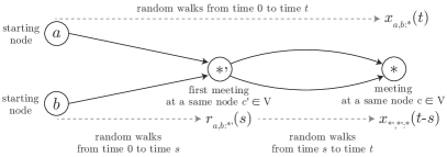
Figure 1: Random walks starting from nodes $a$ and $b$ from time $0$ to time $t$

The right-hand side of Eq. (25) is a convolutional sum, with the consequence that the generating function $X_{a,b:*}(z)$ of $x_{a,b:*}(t)$ is

$$X_{a,b:*}(z)=R_{a,b:*^{\prime}}(z)\,X_{*^{\prime},*^{\prime}:*}(z).$$ (27)

From this equation, the generating function $R_{a,b:*^{\prime}}(z)$ of the first meeting probability $r_{a,b:*}$ is

$$R_{a,b:*^{\prime}}(z)=\frac{X_{a,b:*}(z)}{X_{*^{\prime},*^{\prime}:*}(z)}.$$ (28)

Substituting the spectral formulas of $x_{a:i}(t)$ and $x_{b:i}(t)$ given by Eq. (15) into Eq. (20) yields the following spectral formula for $X_{a,b:*}(z)$:

$$X_{a,b:*}(z)=\sum_{c\in V}\sum_{t=0}^{\infty}x_{a:c}(t)\,x_{b:c}(t)\,z^{t}$$

$$\hskip 2.84544pt=\sum_{c\in V}\frac{d_{c}}{\sqrt{d_{a}d_{b}}}\!\sum_{k=1}^{n}\!\sum_{k^{\prime}=1}^{n}\!q_{k}(a)q_{k}(c)q_{k^{\prime}}(b)q_{k^{\prime}}(c)\!\sum_{t=0}^{\infty}\!\left(\lambda_{k}\lambda_{k^{\prime}}z\right)^{t}$$

$$\hskip 2.84544pt=\sum_{c\in V}\frac{d_{c}}{\sqrt{d_{a}\,d_{b}}}\sum_{k=1}^{n}\sum_{k^{\prime}=1}^{n}\frac{q_{k}(a)\,q_{k}(c)\,q_{k^{\prime}}(b)\,q_{k^{\prime}}(c)}{1-\lambda_{k}\,\lambda_{k^{\prime}}\,z}.$$ (29)

$z$ takes a value within the range of $|\lambda_{k}\,\lambda_{k^{\prime}}\,z|<1$ with the result that the sum of the infinite geometric series converges. From Eq. (26), the generating function $X_{*^{\prime},*^{\prime}:*}(z)$ is

$$X_{*^{\prime},*^{\prime}:*}(z)=\sum_{c^{\prime}\in V}\frac{d_{c^{\prime}}^{2}}{s_{2}}\sum_{c\in V}X_{c^{\prime},c^{\prime}:c}(z).$$ (30)

Substituting the generating function $R_{a,b:*^{\prime}}(z)$ into Eq. (21) results in the expected first meeting time $\mu_{a,b}$ being

$$\mu_{a,b}=\sum_{s=0}^{\infty}s\,r_{a,b:*^{\prime}}(s)=\left.\frac{{\rm d}R_{a,b:*^{\prime}}(z)}{{\rm d}z}\right|_{z=1}.$$ (31)

In this equation, ${\rm d}R_{a,b:*^{\prime}}(z)/{\rm d}z$ is

$$\frac{{\rm d}R_{a,b:*^{\prime}}(z)}{{\rm d}z}=\frac{{\rm d}}{{\rm d}z}\left(\frac{X_{a,b:*}(z)}{X_{*^{\prime},*^{\prime}:*}(z)}\right)$$

$$\hskip 28.45274pt=\frac{\dfrac{{\rm d}X_{a,b:*}(z)}{{\rm d}z}\,X_{*^{\prime},*^{\prime}:*}(z)-X_{a,b:*}(z)\,\dfrac{{\rm d}X_{*^{\prime},*^{\prime}:*}(z)}{{\rm d}z}}{X_{*^{\prime},*^{\prime}:*}^{2}(z)}$$

$$\hskip 28.45274pt=\frac{A(z)-B(z)}{C(z)},$$ (32)

where

$$A(z) =\frac{{\rm d}X_{a,b:*}(z)}{{\rm d}z}\,X_{*^{\prime},*^{\prime}:*}(z),$$ (33)

$$B(z) =X_{a,b:*}(z)\,\frac{{\rm d}X_{*^{\prime},*^{\prime}:*}(z)}{{\rm d}z},$$ (34)

$$C(z) =X_{*^{\prime},*^{\prime}:*}^{2}(z).$$ (35)

According to Eqs. (29) and (30), $A(z)$, $B(z)$, and $C(z)$ can be written as polynomials for $(1-z)$ because of $1-\lambda_{1}\lambda_{1}z=1-z$. Hence, we also obtain $A(z)$ as

$$A(z)=\frac{A_{3}(z)}{(1-z)^{3}}+\frac{A_{2}(z)}{(1-z)^{2}}+\frac{A_{1}(z)}{1-z}+A_{0}(z).$$ (36)

Substituting Eqs. (29) and (30) into the right-hand side of Eq. (33) yields $A_{3}(z)$ and $A_{2}(z)$ as

$$A_{3}(z)\!\! =\!\!\left[\sum_{c\in V}\frac{d_{c}}{\sqrt{d_{a}d_{b}}}q_{1}(a)\,q_{1}^{2}(c)\,q_{1}(b)\right]$$

$$\ \ \ \ \ \ \ \ \ \ \ \ \ \ \left[\sum_{c\in V}\sum_{c^{\prime}\in V}\frac{d_{c^{\prime}}\,d_{c}}{s_{2}}q_{1}^{2}(c)\,q_{1}^{2}(c^{\prime})\right],$$ (37)

$$A_{2}(z)\!\! =\!\!\left[\sum_{c\in V}\frac{d_{c}}{\sqrt{d_{a}d_{b}}}q_{1}(a)\,q_{1}^{2}(c)\,q_{1}(b)\right]$$

$$\ \ \left[\sum_{c\in V}\sum_{c^{\prime}\in V}\!\frac{d_{c^{\prime}}d_{c}}{s_{2}}\!\!\!\!\sum_{\begin{subarray}{c}1\leq k,k^{\prime}\leq n\\ (k,k^{\prime})\neq(1,1)\end{subarray}}\!\!\!\!\frac{q_{k}(c)q_{k}(c^{\prime})q_{k^{\prime}}(c)q_{k^{\prime}}(c^{\prime})}{1-\lambda_{k}\lambda_{k^{\prime}}\,z}\right]$$

$$\!\!\!=\!\!\frac{1}{s_{1}^{2}}\!\!\left[\sum_{c\in V}\sum_{c^{\prime}\in V}d_{c^{\prime}}d_{c}\!\!\!\!\sum_{\begin{subarray}{c}1\leq k,k^{\prime}\leq n\\ (k,k^{\prime})\neq(1,1)\end{subarray}}\!\!\!\!\!\frac{q_{k}(c)q_{k}(c^{\prime})q_{k^{\prime}}(c)q_{k^{\prime}}(c^{\prime})}{1-\lambda_{k}\lambda_{k^{\prime}}z}\right]\!\!.$$ (38)

We do not provide $A_{1}(z)$ and $A_{0}(z)$ in this paper because $A_{1}(z)/(1-z)$ and $A_{0}(z)$ disappear when deriving $\mu_{a,b}$ using Eq. (31). Similarly, $B(z)$ is

$$B(z)=\frac{B_{3}(z)}{(1-z)^{3}}+\frac{B_{2}(z)}{(1-z)^{2}}+\frac{B_{1}(z)}{1-z}+B_{0}(z).$$ (39)

Substituting Eqs. (29) and (30) into the right-hand side of Eq. (34) yields $B_{3}(z)$ and $B_{2}(z)$ as

$$B_{3}(z)\!\! =\!\!\left[\sum_{c\in V}\frac{d_{c}}{\sqrt{d_{a}d_{b}}}q_{1}(a)\,q_{1}^{2}(c)\,q_{1}(b)\right]$$

$$\ \ \ \ \ \ \ \ \ \ \ \ \ \ \left[\sum_{c\in V}\sum_{c^{\prime}\in V}\frac{d_{c^{\prime}}\,d_{c}}{s_{2}}q_{1}^{2}(c)\,q_{1}^{2}(c^{\prime})\right],$$ (40)

$$B_{2}(z)\!\! =\!\!\left[\sum_{c\in V}\sum_{\begin{subarray}{c}1\leq k,k^{\prime}\leq n\\ (k,k^{\prime})\neq(1,1)\end{subarray}}\frac{d_{c}}{\sqrt{d_{a}\,d_{b}}}\frac{q_{k}(a)\,q_{k}(c)\,q_{k^{\prime}}(b)\,q_{k^{\prime}}(c)}{1-\lambda_{k}\lambda_{k^{\prime}}\,z}\right]$$

$$\ \ \ \ \ \ \ \ \ \ \ \ \ \ \ \ \ \ \ \ \ \ \ \ \ \ \ \ \ \ \ \ \ \left[\sum_{c\in V}\sum_{c^{\prime}\in V}\frac{d_{c^{\prime}}\,d_{c}}{s_{2}}q_{1}^{2}(c)\,q_{1}^{2}(c^{\prime})\right]$$

$$=\!\!\frac{1}{s_{1}^{2}}\!\!\left[\sum_{c\in V}\!\frac{d_{c}}{\sqrt{d_{a}\,d_{b}}}\!\!\!\!\sum_{\begin{subarray}{c}1\leq k,k^{\prime}\leq 1\\ (k,k^{\prime})\neq(1,1)\end{subarray}}\!\!\!\!\frac{q_{k}(a)\,q_{k}(c)\,q_{k^{\prime}}(b)\,q_{k^{\prime}}(c)}{1-\lambda_{k}\lambda_{k^{\prime}}\,z}\right].$$ (41)

Using these equations, we have found that $A_{3}(z)=B_{3}(z)$. Consequently, $A(z)-B(z)$ in the numerator of Eq. (32) does not contain the term $(1-z)^{-3}$, with the result that the term $(1-z)^{-2}$ becomes the highest-order term in the polynomials for $(1-z)$ in $A(z)-B(z)$. Thus, $C(z)$ is

$$C(z)=\frac{C_{2}(z)}{(1-z)^{2}}+\frac{C_{1}(z)}{1-z}+C_{0}(z).$$ (42)

Solving this equation in the same manner yields $C_{2}(z)$ as

$$C_{2}(z) =\left[\sum_{c\in V}\sum_{c^{\prime}\in V}\frac{d_{c^{\prime}}\,d_{c}}{s_{2}}q_{1}^{2}(c)\,q_{1}^{2}(c^{\prime})\right]^{2}$$

$$=\left[\frac{1}{s_{1}^{2}}\sum_{c\in V}d_{c}^{2}\right]^{2}=\frac{(s_{2})^{2}}{s_{1}^{4}}.$$ (43)

Since $(A(z)-B(z))/C(z)$ is an indeterminate form at $z=1$, we discuss $\lim_{z\rightarrow 1}(A(z)-B(z))/C(z)$ to derive the spectral formula of the expected first meeting time $\mu_{a,b}$ using Eqs. (31) and (32). As the limit of $z\rightarrow 1$, $\mu_{a,b}$ is

$$\mu_{a,b} =\lim_{z\rightarrow 1}\frac{A(z)-B(z)}{C(z)}=\lim_{z\rightarrow 1}\frac{(1-z)^{2}\!\left(A(z)\!-\!B(z)\right)}{(1-z)^{2}\,C(z)}$$

$$=\frac{A_{2}(1)-B_{2}(1)}{C_{2}(1)}$$

$$=\frac{s_{1}^{2}}{(s_{2})^{2}}\!\!\left[\sum_{c\in V}\sum_{c^{\prime}\in V}\!d_{c^{\prime}}d_{c}\!\!\!\!\!\!\!\!\sum_{\begin{subarray}{c}1\leq k,k^{\prime}\leq n\\ (k,k^{\prime})\neq(1,1)\end{subarray}}\!\!\!\!\!\!\!\!\frac{q_{k}(c)q_{k}(c^{\prime})q_{k^{\prime}}(c)q_{k^{\prime}}(c^{\prime})}{1\!-\!\lambda_{k}\lambda_{k^{\prime}}}\right.$$

$$\left.\ \ \ \ -\sum_{c\in V}\frac{d_{c}}{\sqrt{d_{a}d_{b}}}\!\!\!\!\sum_{\begin{subarray}{c}1\leq k,k^{\prime}\leq 1\\ (k,k^{\prime})\neq(1,1)\end{subarray}}\!\!\!\!\frac{q_{k}(a)\,q_{k}(c)\,q_{k^{\prime}}(b)\,q_{k^{\prime}}(c)}{1\!-\!\lambda_{k}\lambda_{k^{\prime}}}\right]$$

$$=\frac{1}{(s_{2})^{2}}\sum_{c\in V}d_{c}^{2}\sum_{c^{\prime}\in V}d_{c^{\prime}}^{2}\Biggl{[}\Biggr{.}$$

$$s_{1} \sum_{k=2}^{n}\frac{1}{1-\lambda_{k}}\!\left[\frac{2q_{k}(c)q_{k}(c^{\prime})}{\sqrt{d_{c}d_{c^{\prime}}}}\!-\!\frac{q_{k}(c)}{\sqrt{d_{c}}}\!\left(\frac{q_{k}(a)}{\sqrt{d_{a}}}\!+\!\frac{q_{k}(b)}{\sqrt{d_{b}}}\right)\!\right]$$

$$+s_{1}^{2} \Biggl{.}\!\!\!\!\sum_{\begin{subarray}{c}1\leq k,k^{\prime}\leq n\\ (k,k^{\prime})\neq(1,1)\end{subarray}}\!\!\!\!\frac{q_{k}(c)q_{k^{\prime}}(c)}{(1\!-\!\lambda_{k}\lambda_{k^{\prime}})d_{c}}\!\!\left(\!\frac{q_{k}(c^{\prime})q_{k^{\prime}}(c^{\prime})}{d_{c^{\prime}}}\!-\!\frac{q_{k}(a)q_{k^{\prime}}(b)}{\sqrt{d_{a}\,d_{b}}}\!\right)\!\Biggr{]}.$$

Since this equation is expressed by the eigenvalues and eigenvectors of $\bm{W}$, it is the spectral formula of $\mu_{a,b}$.

Equation (LABEL:eq:avg_first_meeting_time_pre) appears to be complicated, but if we use the expected first meeting time $\mu_{a,b:c}$, the time until the two random walkers first meet at node $c\in V$, then $\mu_{a,b}$ is

$$\mu_{a,b} =\frac{1}{s_{2}}\sum_{c\in V}d_{c}^{2}\,\mu_{a,b:c}-\frac{1}{s_{2}^{2}}\sum_{c\in V}d_{c}^{2}\sum_{c^{\prime}\in V}d_{c^{\prime}}^{2}\,\mu_{c^{\prime},c^{\prime}:c},$$

where the spectral formula of $\mu_{a,b:c}$ is

$$\mu_{a,b:c} =\mu_{a:c}+\mu_{b:c}$$

$$+s_{1}^{2}\!\!\!\! \!\!\!\!\sum_{\begin{subarray}{c}1\leq k,k^{\prime}\leq n\\ (k,k^{\prime})\neq(1,1)\end{subarray}}\!\!\!\!\frac{q_{k}(c)q_{k^{\prime}}(c)}{(1\!-\!\lambda_{k}\lambda_{k^{\prime}})d_{c}}\!\!\left(\!\frac{q_{k}(c)q_{k^{\prime}}(c)}{d_{c}}\!-\!\frac{q_{k}(a)q_{k^{\prime}}(b)}{\sqrt{d_{a}\,d_{b}}}\!\right).$$

3. 2 Principal Component of the Expected First Meeting Time $\mu_{a,b}$

We examine the principal component of $\mu_{a,b}$ with the spectral formula of the expected first meeting time $\mu_{a,b}$ and reveal mathematically the effect of the graph structure on the expected first meeting time $\mu_{a,b}$ on the basis of the clarified principal component. We use the method for examining the first hitting time $\mu_{a:i}$ used in [14] to derive the principal component of $\mu_{a,b}$.

First, we introduce

$$\bm{\hat{N}} :=\bm{I}\otimes\bm{I}-\bm{W}\otimes\bm{W}=\bm{\hat{I}}-\bm{\hat{W}},$$ (47)

where $\bm{I}$ is the $n\times n$ unit matrix and $\otimes$ is the Kronecker product. According to the definition of the Kronecker product, $\bm{\hat{I}}$ and $\bm{\hat{W}}$ are $n^{2}\times n^{2}$ matrices. Let $\bm{\hat{N}}^{\dagger}$ be the pseudo-inverse matrix of $\bm{\hat{N}}$ with the result that $\bm{\hat{N}}\bm{\hat{N}}^{\dagger}\bm{\hat{N}}=\bm{\hat{N}}$,

$$\bm{\hat{N}}^{\dagger}=\sum_{\begin{subarray}{c}1\leq k,k^{\prime}\leq n\\ (k,k^{\prime})\neq(1,1)\end{subarray}}\frac{\bm{\hat{q}}_{kk^{\prime}}\,{}^{t}\bm{\hat{q}}_{kk^{\prime}}}{1-\lambda_{k}\lambda_{k^{\prime}}},$$ (48)

where $\bm{\hat{q}}_{kk^{\prime}}$ is the following column vector with $n^{2}$ elements:

$$\bm{\hat{q}}_{kk^{\prime}} :=\bm{q}_{k}\otimes\bm{q}_{k^{\prime}}.$$ (49)

Substituting $\bm{\hat{N}}^{\dagger}$ into Eq. (LABEL:eq:avg_first_meeting_time_pre) yields the following as the expected first meeting time $\mu_{a,b}$:

$$\mu_{a,b} =\frac{s_{1}^{2}}{s_{2}^{2}}\sum_{c\in V}\sum_{c^{\prime}=1}^{n}d_{c}^{2}\,d_{c^{\prime}}^{2}{}^{t}\bm{\hat{u}}_{cc}\bm{\hat{N}}^{\dagger}(\bm{\hat{u}}_{c^{\prime}c^{\prime}}-\bm{\hat{u}}_{ab}).$$ (50)

In this equation, $\bm{\hat{u}}_{ab}$ is

$$\bm{\hat{u}}_{ab} :=\bm{u}_{a}\otimes\bm{u}_{b},$$ (51)

where $\bm{u}_{a}$ is the column vector whose $i$th element $\bm{u}_{a}(i)$ is

$$\bm{u}_{a}(i) =\left\{\begin{array}[]{cc}\displaystyle\frac{1}{\sqrt{d_{a}}}&\mathrm{if}\ \ \ i=a\\ 0&\mathrm{otherwise}\end{array}\right..$$ (54)

The pseudo-inverse matrix $\bm{\hat{N}}^{\dagger}$ of $\bm{\hat{N}}$ in Eq. (48) is also

$$\bm{\hat{N}}^{\dagger} =\sum_{\begin{subarray}{c}1\leq k,k^{\prime}\leq n\\ (k,k^{\prime})\neq(1,1)\end{subarray}}\frac{\bm{\hat{q}}_{kk^{\prime}}\,{}^{t}\bm{\hat{q}}_{kk^{\prime}}}{1-\lambda_{k}\lambda_{k^{\prime}}}$$

$$=\sum_{\begin{subarray}{c}1\leq k,k^{\prime}\leq n\\ (k,k^{\prime})\neq(1,1)\end{subarray}}\frac{(1-\lambda_{k}\lambda_{k^{\prime}}+\lambda_{k}\lambda_{k^{\prime}})\,\bm{\hat{q}}_{kk^{\prime}}\,{}^{t}\bm{\hat{q}}_{kk^{\prime}}}{1-\lambda_{k}\lambda_{k^{\prime}}}$$

$$=\bm{\hat{I}}-\bm{\hat{q}}_{11}{}^{t}\bm{\hat{q}}_{11}+\bm{\hat{M}},$$ (55)

where $\bm{\hat{M}}$ is

$$\bm{\hat{M}} =\sum_{\begin{subarray}{c}1\leq k,k^{\prime}\leq n\\ (k,k^{\prime})\neq(1,1)\end{subarray}}\frac{\lambda_{k}\,\lambda_{k^{\prime}}\,\bm{\hat{q}}_{kk^{\prime}}\,{}^{t}\bm{\hat{q}}_{kk^{\prime}}}{1-\lambda_{k}\lambda_{k^{\prime}}}$$

$$=\sum_{\begin{subarray}{c}1\leq k,k^{\prime}\leq n\\ (k,k^{\prime})\neq(1,1)\end{subarray}}\sum_{s=1}^{\infty}\left(\lambda_{k}\,\lambda_{k^{\prime}}\bm{\hat{q}}_{kk^{\prime}}\,{}^{t}\bm{\hat{q}}_{kk^{\prime}}\right)^{s}$$

$$=\sum_{s=1}^{\infty}\left(\sum_{\begin{subarray}{c}1\leq k,k^{\prime}\leq n\\ (k,k^{\prime})\neq(1,1)\end{subarray}}\lambda_{k}\,\lambda_{k^{\prime}}\bm{\hat{q}}_{kk^{\prime}}\,{}^{t}\bm{\hat{q}}_{kk^{\prime}}\right)^{s}$$

$$=\sum_{s=1}^{\infty}\left(\sum_{k=1}^{n}\sum_{k^{\prime}=1}^{n}\lambda_{k}\,\lambda_{k^{\prime}}\,\bm{\hat{q}}_{kk^{\prime}}\,{}^{t}\bm{\hat{q}}_{kk^{\prime}}-\bm{\hat{q}}_{11}\,{}^{t}\bm{\hat{q}}_{11}\right)^{s}$$

$$=\sum_{s=1}^{\infty}\left(\bm{\hat{W}}-\bm{\hat{q}}_{11}\,{}^{t}\bm{\hat{q}}_{11}\right)^{s}$$

$$=\bm{\hat{W}}\!-\!\bm{\hat{q}}_{11}\!{}^{t}\bm{\hat{q}}_{11}\!+\!\left(\bm{\hat{W}}\!-\!\bm{\hat{q}}_{11}\!{}^{t}\bm{\hat{q}}_{11}\right)^{2}\sum_{s=0}^{\infty}\!\left(\bm{\hat{W}}\!-\!\bm{\hat{q}}_{11}{}^{t}\bm{\hat{q}}_{11}\right)^{s}$$

$$=\bm{\hat{W}}\!-\!\bm{\hat{q}}_{11}{}^{t}\bm{\hat{q}}_{11}\!+\!\left(\bm{\hat{W}}\!-\!\bm{\hat{q}}_{11}{}^{t}\bm{\hat{q}}_{11}\right)^{2}\!\!\!\!\sum_{\begin{subarray}{c}1\leq k,k^{\prime}\leq n\\ (k,k^{\prime})\neq(1,1)\end{subarray}}\!\!\frac{\bm{\hat{q}}_{kk^{\prime}}{}^{t}\bm{\hat{q}}_{kk^{\prime}}}{1\!-\!\lambda_{k}\lambda_{k^{\prime}}}.$$ (56)

This derivation process involved the use of

$${}^{t}\bm{\hat{q}}_{ij}\,\bm{\hat{q}}_{kl} =\left\{\begin{array}[]{ll}1&\mathrm{if}\ i=k\ \mathrm{and}\ j=l\\ 0&\mathrm{otherwise}\end{array}\right.,$$ (59)

$$(\bm{\hat{q}}_{kk^{\prime}}\,{}^{t}\bm{\hat{q}}_{kk^{\prime}})^{s} =\bm{\hat{q}}_{kk^{\prime}}\,{}^{t}\bm{\hat{q}}_{kk^{\prime}}.$$ (60)

Substituting Eq. (55) into Eq. (50) yields the following as $\mu_{a,b}$:

$$\mu_{a,b} =\frac{s_{1}^{2}}{s_{2}}+\frac{s_{1}^{2}}{s_{2}^{2}}\sum_{c\in V}\sum_{c^{\prime}=1}^{n}d_{c}^{2}\,d_{c^{\prime}}^{2}{}^{t}\bm{\hat{u}}_{cc}\bm{\hat{M}}(\bm{\hat{u}}_{c^{\prime}c^{\prime}}-\bm{\hat{u}}_{ab}).$$ (61)

The following was used to obtain this equation:

$${}^{t}\bm{\hat{u}}_{cc} \left(\bm{\hat{N}}^{\dagger}(\bm{\hat{u}}_{c^{\prime}c^{\prime}}-\bm{\hat{u}}_{ab})\right)$$

$$={}^{t}\bm{\hat{u}}_{cc}\left[\left(\bm{\hat{I}}-\bm{\hat{q}}_{11}{}^{t}\bm{\hat{q}}_{11}+\bm{\hat{M}}\right)(\bm{\hat{u}}_{c^{\prime}c^{\prime}}-\bm{\hat{u}}_{ab})\right]$$

$$=\left\{\begin{array}[]{ll}\displaystyle\frac{1}{d_{c}^{2}}+{}^{t}\bm{\hat{u}}_{cc}\bm{\hat{M}}(\bm{\hat{u}}_{c^{\prime}c^{\prime}}-\bm{\hat{u}}_{ab})&\mathrm{if}\ c=c^{\prime}\\ \displaystyle{}^{t}\bm{\hat{u}}_{cc}\bm{\hat{M}}(\bm{\hat{u}}_{c^{\prime}c^{\prime}}-\bm{\hat{u}}_{ab})&\mathrm{otherwise}\\ \end{array}\right..$$ (64)

The first term on the right-hand side of Eq. (61) corresponds to the principal component of the expected first meeting time $\mu_{a,b}$.

To confirm that $s_{1}^{2}/s_{2}$ is the principal component of the expected first meeting time $\mu_{a,b}$, we discuss

$$\left|\frac{\mu_{a,b}}{s_{1}^{2}}-\frac{1}{s_{2}}\right|=\frac{1}{s_{2}^{2}}\sum_{c\in V}\sum_{c^{\prime}=1}^{n}d_{c}^{2}\,d_{c^{\prime}}^{2}\left|{}^{t}\bm{\hat{u}}_{cc}\bm{\hat{M}}(\bm{\hat{u}}_{c^{\prime}c^{\prime}}-\bm{\hat{u}}_{ab})\right|.$$ (65)

The right-hand side of this equation expresses the error between $\mu_{a,b}$ and the principal component $s_{1}^{2}/s_{2}$.

We examine the upper bound on the right-hand side of Eq. (65) using

$$\frac{1}{1-\lambda_{k}\,\lambda_{k^{\prime}}} \leq\frac{1}{1-\lambda_{2}},$$ (66)

for $2\leq k,k^{\prime}\leq n$. Using the above equation, we obtain

$$\left|{}^{t}\bm{\hat{u}}_{cc}\bm{\hat{M}}(\bm{\hat{u}}_{c^{\prime}c^{\prime}}-\bm{\hat{u}}_{ab})\right|$$

$$=\left|{}^{t}\bm{\hat{u}}_{cc}\left(\bm{\hat{W}}\!-\!\bm{\hat{q}}_{11}{}^{t}\bm{\hat{q}}_{11}\right)(\bm{\hat{u}}_{c^{\prime}c^{\prime}}-\bm{\hat{u}}_{ab})\right|$$

$$\ \ +\!\left|{}^{t}\bm{\hat{u}}_{cc}\left(\bm{\hat{W}}\!-\!\bm{\hat{q}}_{11}{}^{t}\bm{\hat{q}}_{11}\right)^{2}\!\!\!\!\!\!\!\sum_{\begin{subarray}{c}1\leq k,k^{\prime}\leq n\\ (k,k^{\prime})\neq(1,1)\end{subarray}}\!\!\!\frac{\bm{\hat{q}}_{kk^{\prime}}{}^{t}\bm{\hat{q}}_{kk^{\prime}}}{1\!-\!\lambda_{k}\lambda_{k^{\prime}}}(\bm{\hat{u}}_{c^{\prime}c^{\prime}}-\bm{\hat{u}}_{ab})\right|$$

$$\leq\left|{}^{t}\bm{\hat{u}}_{cc}\left(\bm{\hat{W}}\!-\!\bm{\hat{q}}_{11}{}^{t}\bm{\hat{q}}_{11}\right)\!(\bm{\hat{u}}_{c^{\prime}c^{\prime}}\!-\!\bm{\hat{u}}_{ab})\right|$$

$$\ \ +\!\frac{1}{1\!-\!\lambda_{2}}\!\left|{}^{t}\bm{\hat{u}}_{cc}\!\left(\!\bm{\hat{W}}\!-\!\bm{\hat{q}}_{11}{}^{t}\bm{\hat{q}}_{11}\right)^{\!2}\!\!\left(\!\bm{\hat{I}}\!-\!\bm{\hat{q}}_{11}{}^{t}\bm{\hat{q}}_{11}\right)\!(\bm{\hat{u}}_{c^{\prime}c^{\prime}}\!-\!\bm{\hat{u}}_{ab})\right|$$

$$=\left|{}^{t}\bm{\hat{u}}_{cc}\bm{\hat{W}}\!(\bm{\hat{u}}_{c^{\prime}c^{\prime}}\!-\!\bm{\hat{u}}_{ab})\right|\!+\!\frac{1}{1\!-\!\lambda_{2}}\left|{}^{t}\bm{\hat{u}}_{cc}\bm{\hat{W}}^{2}(\bm{\hat{u}}_{c^{\prime}c^{\prime}}\!-\!\bm{\hat{u}}_{ab})\right|$$

$$=\left|{}^{t}\bm{\hat{u}}_{cc}\bm{\hat{W}}\!(\bm{\hat{u}}_{c^{\prime}c^{\prime}}\!-\!\bm{\hat{u}}_{ab})\right|\!+\!\frac{1}{1\!-\!\lambda_{2}}\left|\bm{\hat{W}}\bm{\hat{u}}_{cc}\right|\!\left|\bm{\hat{W}}\!(\bm{\hat{u}}_{c^{\prime}c^{\prime}}\!-\!\bm{\hat{u}}_{ab})\right|$$

$$\leq\frac{2\,w_{\mathrm{max}}^{2}}{d_{\mathrm{min}}^{4}}+\frac{1}{1\!-\!\lambda_{2}}\frac{w_{\mathrm{max}}}{d_{\mathrm{min}}^{2}}\frac{\sqrt{2}\,w_{\mathrm{max}}}{d_{\mathrm{min}}^{2}}$$

$$\leq\frac{2\,w_{\mathrm{max}}^{2}}{d_{\mathrm{min}}^{4}}\left(\frac{1}{1\!-\!\lambda_{2}}+1\right).$$ (67)

The following was used in this derivation process:

$$\left|{}^{t}\bm{\hat{u}}_{ij}\bm{\hat{W}}\bm{\hat{u}}_{kl}\right| ={}^{t}\bm{u}_{i}\bm{W}\bm{u}_{k}\otimes{}^{t}\bm{u}_{j}\bm{W}\bm{u}_{l}$$

$$=\frac{w_{ik}}{d_{i}\,d_{k}}\otimes\frac{w_{jl}}{d_{j}\,d_{l}}\leq\frac{w_{\mathrm{max}}^{2}}{d_{\mathrm{min}}^{4}},$$ (68)

$$\left|\bm{\hat{W}}\bm{\hat{u}}_{ij}\right|^{2} ={}^{t}\left(\bm{\hat{W}}\bm{\hat{u}}_{ij}\right)\left(\bm{\hat{W}}\bm{\hat{u}}_{ij}\right)$$

$$=\sum_{k\in\partial i}^{n}\sum_{l\in\partial j}^{n}\frac{w_{ki}^{2}\,w_{lj}^{2}}{d_{k}\,d_{i}^{2}\,d_{l}\,d_{j}^{2}}$$

$$\leq\frac{w_{\mathrm{max}}^{2}}{d_{i}^{2}\,d_{j}^{2}\,d_{\mathrm{min}}^{2}}\sum_{k\in\partial i}^{n}\sum_{l\in\partial j}^{n}w_{ki}\,w_{lj}$$

$$=\frac{w_{\mathrm{max}}^{2}}{d_{i}\,d_{j}\,d_{\mathrm{min}}^{2}}\leq\frac{w_{\mathrm{max}}^{2}}{d_{\mathrm{min}}^{4}}.$$ (69)

Substituting Eq. (67) into Eq. (65) yields the following as the upper bound of the error between $\mu_{a,b}$ and the principal component $s_{1}^{2}/s_{2}$:

$$\left|\frac{\mu_{a,b}}{s_{1}^{2}}-\frac{1}{s_{2}}\right|\leq\frac{2\,w_{\mathrm{max}}^{2}}{d_{\mathrm{min}}^{4}}\left(\frac{1}{1-\lambda_{2}}+1\right).$$ (70)

According to this equation, the error can be expected to be small for graph $G$, where $\lambda_{2}$ and $w_{\mathrm{max}}$ are small but $d_{\mathrm{min}}$ is large. In this case, the expected first meeting time $\mu_{a,b}$ is approximated as

$$\mu_{a,b}\approx\frac{s_{1}^{2}}{s_{2}}=\frac{n}{1+d_{\rm std}^{2}/d_{\rm avg}^{2}},$$ (71)

where $d_{\rm avg}$ and $d_{\rm std}$ are the average and standard deviation of weighted degrees, respectively.

If the approximation formula (71) holds for the expected first meeting time $\mu_{a,b}$, we derive the following characteristics: (a) $\mu_{a,b}$ is small when the coefficient of variation $d_{\rm std}/d_{\rm avg}$ is large and (b) $\mu_{a,b}$ does not depend on the starting nodes $a$ and $b$. The characteristic (a) is useful for understanding the effect of the graph structure on $\mu_{a,b}$.

4 Numerical Example

In this section, we confirm the validity of the spectral formula (LABEL:eq:avg_first_meeting_time_pre) and the principal component of the expected first meeting time $\mu_{a,b}$ revealed in Sect. 3. We also examine the error in the approximation formula (71) obtained when $\mu_{a,b}$ is replaced by its principal component.

4. 1 Setting

In this subsection, we use BA (Barabási-Albert) graphs [15] and ER (Erdös-Rényi) graphs [16]. The spectral formula (LABEL:eq:avg_first_meeting_time_pre) and the approximation formula (71) depend on the degree distribution of a graph. Since the degree distribution of a BA graph is different from that of an ER graph, these graphs are useful for clarifying the effects of the degree distribution on these formulas. Owing to space limitations, we provide the results for unweighted graphs, where $w_{ij}=1$ is provided for all links $\forall(i,j)\in E$. In unweighted graphs, the weighted degree $d_{i}$ of node $i$ corresponds to the degree $m_{i}$, the number of links of node $i$.

The BA model [15] is a typical model for scale-free random graphs. A BA graph is generated using the following procedure. First, a complete graph with $n_{0}$ nodes is created. We assume that $n_{0}=m$ for the sake of simplicity. Next, nodes are inserted one by one until the number of nodes in the BA graph is equal to $n$. When adding the $t$th node ($t=m+1,m+2,\cdots,n$), $m_{\rm new}$ links are created from node $t$ to nodes $j\in\{1,2,\cdots,t-1\}$ with the connection probability $p^{\mathrm{BA}}_{j}(t)$. The connection probability $p^{\mathrm{BA}}_{j}(t)$ is

$$p^{\mathrm{BA}}_{j}(t)=\frac{m_{j}(t)}{\sum_{l=1}^{t-1}m_{l}(t)},$$ (72)

where $m_{j}(t)$ is the degree of node $j$ when the insertion of the $t-1$th node is completed. BA graphs have the power-law degree distribution (i.e, ${\rm Prob}\left[m_{i}=m\right]\sim m^{-3}$). If $G$ is unweighted, then the average weighted degree $d_{\rm avg}$ is equal to the average degree $k_{\rm avg}$. Hence, the average weighted degree $d_{\rm avg}$ of a BA graph is approximated as

$$d_{\rm avg}=\frac{m\,(m-1)+2\,m\,(n-m)}{n}\approx 2\,m,$$ (73)

where we assume that $n\gg m$.

In contrast, the ER model [16] is a classical random graph model. An ER graph is generated through the following procedure. First, $n$ nodes are created. Next, links are created between any pair of nodes with probability $p^{\mathrm{ER}}$. If the graph is not connected, then the link creation process is begun again. The average weighted degree $d_{\rm avg}$ of an ER graph is

$$d_{\rm avg} =(n-1)\,p^{\mathrm{ER}}.$$ (74)

The degree distribution ${\rm Prob}\left[m_{i}=m\right]$ of an ER graph follows the binomial distribution. According to the difference between the power law and the binomial distribution, the standard deviation $d_{\rm std}$ of weighted degrees in a BA graph is greater than that in an ER graph.

To focus on the difference in the standard deviation $d_{\rm std}$ of weighted degrees, we set $m$ and $p^{\mathrm{ER}}$ as

$$m =\left\lfloor\frac{d_{\rm avg}}{2}\right\rfloor,$$ (75)

$$p_{\rm ER} =\frac{d_{\rm avg}}{n-1},$$ (76)

with the result that the average weighted degree $d_{\rm avg}$ of an ER graph and a BA graph are roughly equal. The minimum weighted degree $d_{\rm min}$ in both graphs also increases as $d_{\rm avg}$ increases.

To examine the validity and the error of the spectral formula (LABEL:eq:avg_first_meeting_time_pre) and the approximation formula (71), we measure the average of the first meeting times in simulation using the following procedure.

1. Generate a BA graph or an ER graph using the above procedures.

2. Put random walkers on nodes $a\in V$ and $b\in V$.

3. Move each random walker with the transition probability $p_{i\rightarrow j}$ in accordance with Eq. (2).

4. Repeat step 3 until the two random walks meet at the same node.

5. Repeat step 2 through step 4 10,000 times to calculate the average of the first meeting times.

We use the parameter configuration shown in Tab. 1 as a default parameter configuration.

Table 1: Parameter configuration

Number of nodes	$n$	1,000
Weight of link $(i,j)$	$w_{ij}$	1
Average weighted degree	$d_{\mathrm{avg}}$	6
Random walker’s starting node	$a$	1

4. 2 Validity of the Spectral Formula for the Expected First Meeting Time $\mu_{a,b}$

We confirm the validity of the spectral formula of the expected first meeting time $\mu_{a,b}$ given by Eq. (LABEL:eq:avg_first_meeting_time_pre).

Figures 2 and 3 show the first meeting times obtained from the simulation and the analysis (i.e., the spectral formula (LABEL:eq:avg_first_meeting_time_pre)) for different settings of the random walker’s starting node $b$ in the BA and ER graphs, respectively. According to Figs. 2 and 3, the analysis results are almost the same as the simulation results regardless of the choice of $n$ and $b$.

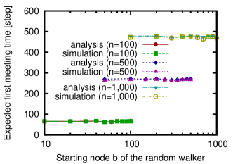
Figure 2: Expected first meeting time $\mu_{a,b}$ for different settings of the starting node $b$ of the random walker in BA graphs

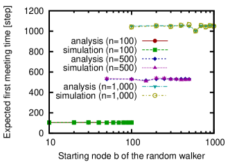
Figure 3: Expected first meeting time $\mu_{a,b}$ for different settings of the starting node $b$ of the random walker in ER graphs

We then evaluate the error in the spectral formula (LABEL:eq:avg_first_meeting_time_pre). In this evaluation, we use the relative error $\epsilon_{a,b}$ of the expected first meeting time $\mu_{a,b}$. The relative error $\epsilon_{a,b}$ is defined as

$$\epsilon_{a,b}:=\frac{\left|\mu_{a,b}-\mu_{a,b}^{\mathrm{sim}}\right|}{\mu_{a,b}^{\mathrm{sim}}},$$ (77)

where $\mu_{a,b}^{\mathrm{sim}}$ is the average of the first meeting times obtained from the simulation. We examine the average and the maximum of the relative errors $\epsilon_{a,b}$ when changing starting node $b$ while the starting node $a$ is fixed.

Figure 4 shows the average and the maximum of the relative errors $\epsilon_{a,b}$ of the expected first meeting time $\mu_{a,b}$ in the BA and ER graphs with different settings of the average weighted degree $d_{\mathrm{avg}}$. In this figure, we do not plot the results for the ER graphs with $d_{\mathrm{avg}}=2$ and $4$, because a connected ER graph cannot be generated. According to Fig. 4, if $d_{\mathrm{avg}}\geq 4$, then the maximum of relative errors $\epsilon_{a,b}$ is only a few percent. Therefore, the spectral formula (LABEL:eq:avg_first_meeting_time_pre) is valid for the graphs with $d_{\mathrm{avg}}\geq 4$.

Figure 4: Average weighted degree $d_{\mathrm{avg}}$ vs. the average and the maximum of the relative error $\epsilon_{a,b}$ for the expected first meeting $\mu_{a,b}$

We discuss the reason that the relative error $\epsilon_{a,b}$ is large when we use a BA graph with a small-average weighted degree (i.e., $d_{\mathrm{avg}}=2$). In Sect. 3, we use Eq. (26) to derive the spectral formula (LABEL:eq:avg_first_meeting_time_pre). Equation (26) assumes that the first meeting probability of two random walkers at node $c$ is proportional to $d_{c}^{2}$. Hence, we confirm the acceptance of this assumption to clarify the reason for the large relative error.

Figures 5 (a) through (c) show scatter plots of the first meeting frequency of two random walkers at node $c$ in BA graphs with different settings of the average weighted degree $d_{\mathrm{avg}}$. The first meeting frequency at each node was obtained from the simulation, where the starting nodes $a$ and $b$ are fixed. In order to confirm easily the correctness of the assumption, we plot the fitting curve of $d_{c}^{2}$ in these figures. According to Figs. 5 (a) through (c), the first meeting frequencies with $d_{\mathrm{avg}}=2$ differ only largely from the fitting curve, with the consequence that the assumption must not be accepted for the cases with $d_{\mathrm{avg}}=2$. Therefore, we conclude that the large relative error shown in Fig. 4 is caused by the assumption for Eq. (26).

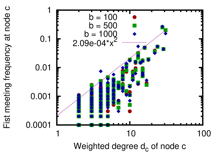
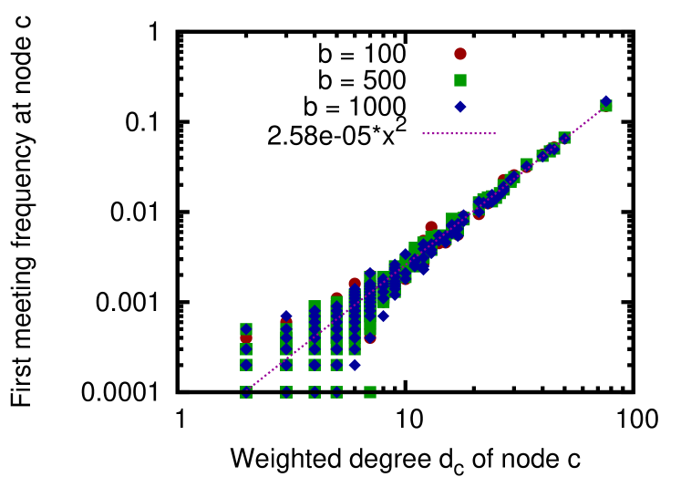
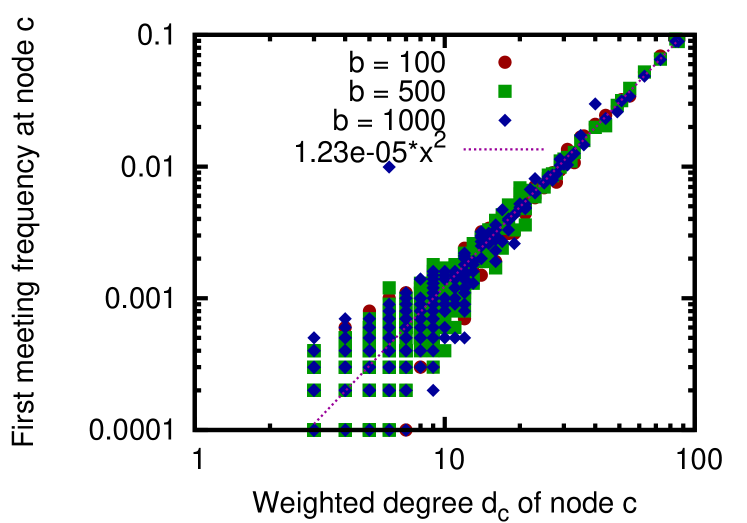
$d_{\mathrm{avg}}=2$ $d_{\mathrm{avg}}=4$ $d_{\mathrm{avg}}=6$

Figure 5: Weighted degree $d_{c}$ of node $c$ vs. the first meeting frequency at node $c$ in BA graphs

According to the results, the spectral formula of first meeting time $\mu_{a,b}$ will be valid if the average weighted degree $d_{\mathrm{avg}}$ is sufficiently large (i.e., $d_{\mathrm{avg}}\geq 4$).

4. 3 Validity for the Principal Component of the Expected First Meeting Time $\mu_{a,b}$

We clarify the validity for the principal component of the expected first meeting time $\mu_{a,b}$ derived in Sect. 3. Specifically, we examine the relative error $\epsilon_{a,b}^{\prime}$ of the approximation formula (71) obtained when the expected first meeting time $\mu_{a,b}$ is given by the principal component (i.e., $s_{1}^{2}/s_{2}$). The relative error $\epsilon_{a,b}^{\prime}$ is defined as

$$\epsilon_{a,b}^{\prime}:=\frac{\left|\frac{s_{1}^{2}}{s_{2}}-\mu_{a,b}^{\mathrm{sim}}\right|}{\mu_{a,b}^{\mathrm{sim}}}.$$ (78)

Figures 6 and 7 show the averages of the relative errors $\epsilon_{a,b}^{\prime}$ of the approximation formula (71) for BA and ER graphs with different numbers of nodes, $n$, respectively. The average of the relative errors $\epsilon_{a,b}^{\prime}$ was calculated from 10,000 simulations, where the starting nodes $a$ and $b$ are selected randomly. In Fig. 7, we do not plot the result for $n=10,000$ and $d_{\mathrm{avg}}=6$, because a connected ER graph cannot be generated. According to the results, if the average weighted degree $d_{\mathrm{avg}}$ is sufficiently large, the relative error $\epsilon_{a,b}^{\prime}$ is small, and the derived principal component is valid. This can also be explained by Eq. (70). The right-hand side of Eq. (70) represents the upper bound of the error in the approximation formula (71). If the average weighted degree $d_{\mathrm{avg}}$ is large, the minimum weighted degree $d_{\rm min}$ is also large. As the minimum weighted degree $d_{\rm min}$ increases, the upper bound becomes small, and the relative error $\epsilon_{a,b}^{\prime}$ of the approximation formula (71) can be expected to decrease. Moreover, according to Figs. 6 and 7, the average of the relative errors $\epsilon_{a,b}^{\prime}$ is constant or becomes smaller as $n$ increases, and hence the approximation formula (71) is also effective for large-scale graphs.

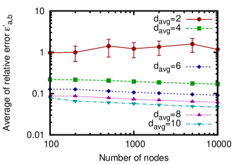
Figure 6: Number of nodes, $n$, vs. the average of the relative errors $\epsilon_{a,b}^{\prime}$ of the approximation formula (71) in the BA graphs

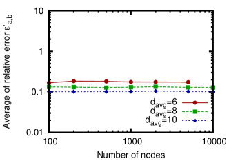
Figure 7: Number of nodes, $n$, vs. the average of the relative errors $\epsilon_{a,b}^{\prime}$ of the approximation formula (71) in the ER graphs

From the above results, the derived principal component is valid if the average weighted degree $d_{\mathrm{avg}}$ is sufficiently large (i.e., $d_{\mathrm{avg}}\geq 4$). According to the site [17], which collecting statistical information (e.g., average degree) of various existing graphs, the average degree of a typical graph is greater than four. Hence, our analysis results are expected to be useful for many real graphs.

Finally, we confirm the effect of the graph structure on the expected first meeting time $\mu_{a,b}$ revealed in Sect. 3. According to the approximation formula (71), $\mu_{a,b}$ increases as $s_{1}^{2}/s_{2}$ increases. To confirm the effect from the numerical example, we compare $s_{1}^{2}/s_{2}$ and the average of the first meeting times obtained in the simulation.

Figures 8 and 9 show the averages of the first meeting times obtained from the simulation with different settings of $s_{1}^{2}/s_{2}$ in the BA and ER graphs, respectively. To calculate the average of the first meeting times, we conduct 10,000 simulations, where the starting nodes $a$ and $b$ are selected randomly. In these figures, we plot the straight line for $y=x$ to confirm the effect easily. According to the results, the average of the first meeting times is approximately along the $y=x$ line, except for the result for BA graphs with average weighted degree $d_{\mathrm{avg}}=2$. Therefore, the effect is also confirmed from the numerical example if the average weighted degree $d_{\mathrm{avg}}$ is sufficiently large.

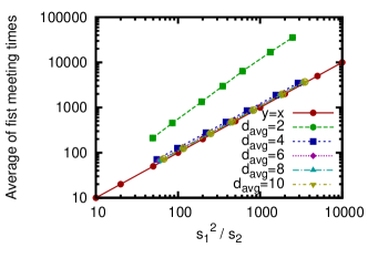
Figure 8: Principal component $s_{1}^{2}/s_{2}$ vs. the average of the first meeting times in the BA graphs

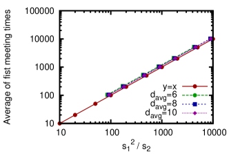
Figure 9: Principal component $s_{1}^{2}/s_{2}$ vs. the average of the first meeting times in the ER graphs

5 Conclusion and Future Work

In this paper, we analyzed the first meeting time of multiple random walks in arbitrary graphs and clarified the effects of graph structures on its expected value. First, we derived the spectral formula of the expected first meeting time for two random walkers using spectral graph theory. Then, we examined the principal component of the expected first meeting time using the derived spectral formula. The clarified principal component reveals that (a) the expected first meeting time is almost dominated by $n/(1+d_{\rm std}^{2}/d_{\rm avg}^{2})$, and (b) the expected first meeting time is independent of the starting nodes of random walkers, where $n$ is the number of nodes. $d_{\rm avg}$ and $d_{\rm std}$ are the average and the standard deviation of the weighted degree, respectively. The characteristic (a) is useful for understanding the effect of the graph structure on the first meeting time. In addition, we confirmed the validity of the analysis results through numerical examples. According to the revealed effects of the graph structures, the variance of the coefficient for weighted degrees, $d_{\rm std}/d_{\rm avg}$ (degree heterogeneity), facilitates the meeting of random walkers.

As future work, we plan to examine the validity of the analysis results with real graphs and apply them to the development of efficient graph algorithms.

Yusuke Sakumoto received M.E. and Ph.D. degrees in the Information and Computer Sciences from Osaka University in 2008 and 2010, respectively. From 2010 to 2019, he was a associate professor of Tokyo Metropolitan University. He is currently an associate professor at Kwansei Gakuin University. His research work is in the area of analysis of communication network and social network. He is a member of the IEEE, IEICE and IPSJ.

Hiroyuki Ohsakireceived the M.E. degree in the Information and Computer Sciences from Osaka University, Osaka, Japan, in 1995. He also received the Ph.D. degree from Osaka University, Osaka, Japan, in 1997. He is currently a professor at Department of Informatics, School of Science and Technology, Kwansei Gakuin University, Japan. His research work is in the area of design, modeling, and control of large-scale communication networks. He is a member of IEEE and Institute of Electronics, Information, and Computer Engineers of Japan (IEICE).

References

- [1] Q. Lv, P. Cao, E. Cohen, K. Li, and S. Shenker, “Search and replication in unstructured peer-to-peer networks,” in Proceedings of the 16th ACM international conference on Supercomputing (ICS’02), Jun. 2002, pp. 84–95.
- [2] C. Gkantsidis, M. Mihail, and A. Saberi, “Random walks in peer-to-peer networks,” in Proceedings of the 23rd Conference of the IEEE Communications Society (INFOCOM 2004), Mar. 2004, pp. 120–130.
- [3] C. Dutta, G. Pandurangan, R. Rajaraman, and S. Roche, “Coalescing-branching random walks on graphs,” ACM Transactions on Parallel Computing (TOPC), vol. 2, no. 3, pp. 1–29, Nov. 2015.
- [4] Y. Metivier, N. Saheb, and A. Zemmari, “Randomized rendezvous,” Mathematics and Computer Science, pp. 183–194, 2000.
- [5] A. Israeli and M. Jalfon, “Token management schemes and random walks yield self-stabilizing mutual exclusion,” in Proceedings of the 9th Annual ACM Symposium on Principles of Distributed Computing (PODC ’90). ACM, Aug. 1990, pp. 119–131.
- [6] P. Tetali and P. Winkler, “On a random walk problem arising in self-stabilizing token management,” in Proceedings of the 10th annual ACM symposium on Principles of distributed computing (PODC ’91). ACM, Aug. 1991, pp. 273–280.
- [7] D. Coppersmith, P. Doyle, P. Raghavan, and M. Snir, “Random walks on weighted graphs and applications to on-line algorithms,” Journal of the ACM, vol. 40, no. 3, pp. 421–453, Jul. 1993.
- [8] D. J. Aldous, “Meeting times for independent markov chains,” Stochastic Processes and their Applications, vol. 38, no. 2, pp. 185–193, Aug. 1991.
- [9] N. H. Bshouty, L. Higham, and J. Warpechowska-Gruca, “Meeting times of random walks on graphs,” Information Processing Letters, vol. 69, no. 5, pp. 259–265, 1999.
- [10] C. Cooper, A. Frieze, and T. Radzik, “Multiple random walks in random regular graphs,” SIAM Journal on Discrete Mathematics, vol. 23, no. 4, pp. 1738–1761, Jun. 2009.
- [11] Y. Zhang, Z. Tan, and B. Krishnamachari, “On the meeting time for two random walks on a regular graph,” arXiv preprint arXiv:1408.2005, 2014.
- [12] M. George, R. Patel, and F. Bullo, “The meeting time of multiple random walks,” Preprint submitted to Linear Algebra and Its Applications, Mar. 2017, available at http://motion.me.ucsb.edu/pdf/2014l-gpb.pdf.
- [13] L. Lovász, “Random walks on graphs: a survey,” Combinatorics, Paul Erdős is eighty, vol. 2, pp. 353–398, 1996.
- [14] U. Von Luxburg, A. Radl, and M. Hein, “Hitting and commute times in large graphs are often misleading,” arXiv preprint arXiv:1003.1266, May 2011.
- [15] A. L. Bárabasi and R. Albert, “Emergence of scaling in random networks,” Science, vol. 286, no. 5439, pp. 509–512, Oct. 1999.
- [16] P. Erdös and A. Rényi, “On random graphs,” Mathematicae, vol. 6, no. 26, pp. 290–297, 1959.
- [17] J. Kunegis, “The koblenz network collection (KONECT),” http://konect.uni-koblenz.de/ (accessed on May 29, 2020).