Wavelet analysis of the long-term activity of V833 Tau

Abstract

The bulk of available stellar activity observations is frequently checked for the manifestation of signs in comparison with the known characteristic of solar magnetic modulation. The problem is that stellar activity records are usually an order of magnitude shorter than available observations of solar activity variation. Therefore, the resolved time scales of stellar activity are insufficient to decide reliably that a cyclic variation for a particular star is similar to the well-known 11-yr sunspot cycles. As a result, recent studies report several stars with double or multiple cycles which serve to challenge the underlying theoretical understanding. This is why a consistent method to separate ’true’ cycles from stochastic variations is required. In this paper, we suggest that a conservative method, based on the best practice of wavelet analysis previously applied to the study of solar activity, for studying and interpreting the longest available stellar activity record – photometric monitoring of V833 Tau for more than 100 years. We find that the observed variations of V833 Tau with timescales of 2 – 50 yr should be comparable with the known quasi-periodic solar mid-term variations, whereas the true cycle of V833 Tau, if it exists, should be of about a century or even longer. We argue that this conclusion does not contradict the expectations from stellar dynamo theory.

1 Introduction

Spatial and temporal variations in the activity of stars and, especially, the Sun are the obvious manifestations of complicated processes in turbulent magnetoconvection. The understanding of mechanisms that underlie many of these processes is still a major open issue in astrophysics. The dynamo problem remains a key challenge despite the fact that the pioneering formulation of the principal ”mechanism“ (Parker, 1955) has long been developed theoretically and verified experimentally. There are also many related problems of theoretical and practical interests, for example, coronal heating (see for review Testa et al. (2015)), stellar flare oscillations (Doyle et al., 2018) or seismic signatures (Salabert et al., 2016; Kiefer et al., 2019). A comparison of stellar and solar activity is a natural line of research (Schrijver & Zwaan, 2008). The possibilities of observing solar activity are significantly superior in accuracy and in the variety of available tools than those associated with measuring stellar activity. The study of a wide population of Sun-like stars has the advantage of providing a distribution of control parameters Vidotto et al. (2014), which makes results more meaningful and robust for assessing various theories and models.

Important systematic observations of stellar activity were accomplished by the well-known HK project at the Mount Wilson Observatory (MWO) that began in 1966 and lasted over three decades (Baliunas et al., 1995). Chromospheric Ca II H+K emission in narrow passbands were measured for almost 100 stars. Other programs at the Lowell Observatory (1984-2000) and Fairborn Observatories (1993-2003) continued studying the (year-to-year) Strömgren b, y photometric variability of a sample of 30+ stars (Lockwood et al., 1997; Radick et al., 1998). The Solar-Stellar Spectrograph is a project (since 1994) dedicated to long-term observations of the Sun and Sun-like stars with the same instrument at Lowell Observatory (Hall & Lockwood, 1995). Recent space-based asteroseismology missions such as MOST (Walker et al., 2003), CoRoT (Auvergne et al., 2009), and Kepler (Borucki et al., 2010), as well as ground-based networks like the Stellar Observations Network Group (SONG; Grundahl et al. (2008)), contribute a lot of complementary data for solar-type stars.

The well recognized 11-yr solar cycle (also known as the Schwabe sunspot cycle) is a distinctive timescale in comparison with other time scales of solar activity (Hathaway, 2015). It is natural to attempt to identify pronounced cyclic activity in other stars. However, available observational data for any particular star remained much smaller than that for the continuous observation and study of sunspot activity. This observational deficiency indeed complicates any direct solar-stellar comparison. The telescopic recordings of sunspot activity available for the past four centuries tell us that the observation of any particular cycle or even pair of cycles would not be sufficient to develop the comprehensive dynamo model which we have so far. Solar dynamo as a physical process representing the underlying solar magnetic activity includes a dominant eigen-mode of corresponding mean-field equations as an explanation of the 11-yr cycle. Various nonlinear effects or purely turbulent variations cause significant amplitude and period modulations of the 11-yr cycle (Frick et al., 2020). In principle, spherical dynamos can include several dynamo active shells and manifest a transition from axi- to nonaxisymmetric dynamo modes (Viviani et al., 2018). However, it is a very demanding assumption and one shell can enslave another one and hence reducing the number of independent eigen-modes (e.g. Moss & Sokoloff, 2007). Penetration of the activity wave from the lower shells up to the surface is another difficulty associated with the available schemes of solar activity (e.g. Moss et al., 2011). The observation of non solar-like stellar activity is a motivating reason for considering the dynamo model with anti-solar differential rotation, in which the equator rotates slower than poles (Karak et al., 2020). The identification of long-term stellar activity variations with dynamo cycles is of crucial importance for their interpretation and modelling (Lehmann et al., 2018).

However, the stellar data available for some stars demonstrate clear quasi-stable cycles (e.g., HD81809 or HD10476 in Frick et al. (2004)), whereas other data illustrate a periodicity that varies substantially even during the full records of several oscillations (e.g., HD201092, HD219834A in Frick et al. (2004)). It is difficult to conclude that a given set of observations identifies a clear solar-type cycle if only two or three cycles are covered Kiefer et al. (2017). Moreover, a solar-stellar comparison becomes more complicated due to the necessity to take into account stellar mass, age, rotation rate and orientation of the rotation axes. Having no solar “identical twin”, we cannot be sure that the observed stellar activity is truly another “solar experiment”. The Kepler mission has provided a data sample of 4000 Sun-like stars with measured rotation periods. About 10% of these stars have long-term variability in their observed fluxes. Although the full records did not exceed 4.5 years, nevertheless one can identify a sample of stars with apparently complete cycles (Montet et al., 2017; Karoff et al., 2019).

One more point here is that the main bulk of the examined stellar cycles has the length of the order of the Schwabe cycle or shorter. It looks like a selection effect will be introduced because of the limited length of the available observational time series. Therefore, it is essential to have a method that may allows one to isolate the cases where one can deduce at least a lower estimate for a long-term activity cycle period despite the fact that the true periods cannot be accessible just yet from the available observations Vida et al. (2016). The desired method should explain why the shorter time scales presented in the time series of interest should be considered as something else rather than the main activity period comparable with the Schwabe cycle. It is hard to conclude that a star is exhibiting a type of Maunder Minimum like activity phase based on observations of low activity over a short time span (cf. Hall et al., 2009).

We note that even the 400-year period of instrumental observations of sunspot activity has not finalized the discussion concerning the physical status of various time scales isolated in the solar activity record, and that the cycles supplementary to the main Schwabe cycle are still debatable. We emphasized here that the example of a star with a record of 10 time scales can be more valuable than 10 records of different stars with a length of one time scale. In fact, we have patterns of variation for the Sun and 72 sun-like stars over 1-3 decades but its solar-like behaviour is still questionable (Radick et al., 2018). The aim of this paper is to develop a conservative method for the interpretation of the multi-timescale stellar activity using wavelet based techniques. As an instructive example, we analyzed the data of the longest available stellar activity – photometric monitoring of V833 Tau. These data can provide a first direct evidence that the star may have an activity period of about a century long.

2 V833 Tau: general properties

V833 Tau (GJ 171.2A or HD 283750) is a single-lined spectroscopic binary; the second component was detected by Heintz (1981). The orbital elements of the system are determined by Griffin et al. (1985), and described in more detail by Halbwachs et al. (2000); Halbwachs et al. (2018). The second star (HD 283750b) is moving on the circular orbit with a period of 1.788011 d, its mass is estimated to be about 0.17 $M_{\odot}$ or less, and it is consistent with being a brown dwarf. The infrared spectroscopic study by Lucas & Roche (2002) allows one to consider HD 283750b as a hot Jupiter planet with mass of 50 $M_{\rm Jup}$. Griffin et al. (1985) presented the history of the study of HD 283750.

Eggen & Sandage (1965) found that the brightness of the star CJ171.2 A is $V=8.42^{m}$ and the spectral type is dK5pe with emission in hydrogen lines. Its photometric and spectroscopic features correspond to the BY Dra type variables (Bopp et al., 1981). The rotation modulation with the period of 1.85 d was found by Pettersen (1989), and later this value was refined by photometric observations from 1987-2000 (Olah & Pettersen, 1991; Oláh et al., 2001). The adopted $P_{\rm rot}=1.7940$ d is close to the orbital period $P_{\rm orb}=1.787992$ d (Halbwachs et al., 2000). The system is in synchronous rotation, but the photometric rotational period changes slightly due a migration of starspots over the main cycle. The differential rotation appears to be the same as that on the Sun (Olah & Pettersen, 1991; Bondar’, 2017), but Alekseev (2005) has proposed an anti-solar type of differential rotation.

In modeling starspots and determining the activity level, the following general parameters of the star are being adopted. The spectral type of the star is usually accepted to be K5 (Gliese & Jahreiß, 1991) or K2 (Oswalt et al., 1988; Oláh et al., 2001), however Scholz et al. (2018) recorded the spectral type as K3 IV. Accordingly, Pettersen (1989) observed $T_{\rm eff}=4450$ K, $R=0.77$ $R_{\odot}$, $log(L/L_{\odot})=-0.68$, $M=0.8$ $M_{\odot}$ (Hartmann et al., 1981; Strassmeier et al., 1993), an inclination $i=20^{\circ}$ (Olah & Pettersen, 1991). Oláh et al. (2001) considered the model in which a large polar spot and some small spots on low latitudes are present on the stellar surface and cover, in general, a significant part of the photosphere, up to 30-50%. Alekseev & Bondar’ (1998) derived spots areas up to 40% assuming that their distribution is concentrated in the equatorial zone (Alekseev & Gershberg, 1997).

The long-term photometric data, received for some decades from archives of the photographic measurements (Hartmann et al., 1981; Bondar’, 1995), revealed the starspots cycle of activity of this star. The length of the cycle was estimated to be about 60 yr and the cycle amplitude exceeds 0.6^m, which is an indication of a high level of photospheric activity, the largest among the known red dwarfs.

3 Photometric behavior of V833 Tau in some decades and suspected activity cycles

The specific feature of the photometric behavior of V833 Tau on timescale of decades is a significant change in the star brightness, up to 0.6-0.8^m in the $V$-band relative to the unspotted maximum level (Bondar’ et al., 2019). Oláh et al. (2001) accepted $V_{\rm max}=7.90^{m}$ based on observation during the 1987-2000 interval, and Bondar’ (2015) found $V_{\rm max}=7.94^{m}$ from the long observational data over 1899-2009. The stellar magnitude of an active star in its quiescent stage, i.e. without flares and spots, is a very important value in order to determine parameters of starspots and to model a light curve. This parameter can be found by using the long-term photometry or by analyzing the models of stellar atmospheres for a given spectral type.

The time span between the consecutive unspotted states is considered as the length of a possible cycle of activity. To seek such stellar activity cycles, the data rows obtained for several decades are required. At present, the chromospheric activity of 29 stars from the MWO HK project have been monitored over 36 yr (Oláh et al., 2016). The study of photospheric activity is based on various photometric sources that allow one to form a combined light curve over long time intervals.

The measurements by Hartmann et al. (1981) in the Harvard University’s archive plate collection and by Bondar’ (1995) in the photographic archive of the Sternberg Astronomical Institute (Moscow State University) made it possible to consider the photometric behavior of the star since 1899. The photographic $B$-magnitudes are used to add other photometric data and to construct a common light curve. In our studies, the combined light curve of V833 Tau based on its own and published photometric data, the $V$-magnitudes from photometric data bases ASAS (Pojmanski, 1997), SuperWASP (https://wasp.cerit-sc.cz/form) and the Kamogata Wide-Field Survey (KWS, http://kws.cetus-net.org/~maehara/VSdata.py?object) are used.

Oláh et al. (2001) made analysis of the available photographic and photoelectric $B$ measurements from 1899 to 2000 and determined the main activity cycle to be as long as 67-69 yr. From the more precise photoelectric light curve over 1987-2000 interval they found shorter cycles of 6.5 yr and 2.4 yr. The authors noted that the multiplicity of cycles emphasizes a similarity between the V833 Tau and the Sun. Bondar’ (2015) analysed the yearly-mean $B$-magnitudes on the interval of 1899-2009 searching for periodic changes using the statistical package AVE (http://www.astrouw.edu.pl/asas/?page=acvs). The results obtained allowed one to suspect a long activity cycle of 78.25 yr with the large amplitude of 0.6^m. After the removal of this long period, the period of 18.8 yr with amplitude of 0.2-0.4^m was found. Five waves of this cycle were traced on the investigated timespan; however, their form, phase of minimum and amplitude change from cycle to cycle. The residuals after accounting for the contribution of the 18.8 yr period showed the presence of shorter cycles of 6.4 yr and 2.5 yr long (similar to Oláh et al., 2001) with amplitudes less than 0.07^mc. Apparently, the same cycles can be obtained from the analysis of the $V$-light curve because the $V$-and $B$-magnitudes are related.

In this work, we study changes in the brightness of the star over the full 1899-2019 interval. The photographic $B$-magnitudes were transformed to $V$-magnitudes using the accepted mean value $B-V=1.07$ (Bondar’, 2015). The yearly-mean $V$-magnitudes were obtained as described above. Figure 1 shows the light curve of the star, symbols indicate data sources, and bars show standard error deviations. Photographic measurement errors are large, up to $0.15^{m}$, and the errors of more modern photometry measurements are usually less than 0.04^m.

As follows from the light curve (see Fig. 1), the high levels of brightness of V833 Tau ($V=8.00^{m}$) were reached during the 1918-1921 and 1976-1977 intervals, and it was even slightly higher ($V=7.89^{m}$) during 1997-2000. A remarkable decrease in the brightness began in 1928 and continued up to 1968 when the stellar magnitude was not more than 8.4^m, and the deep minima were observed around 1935 and 1950.

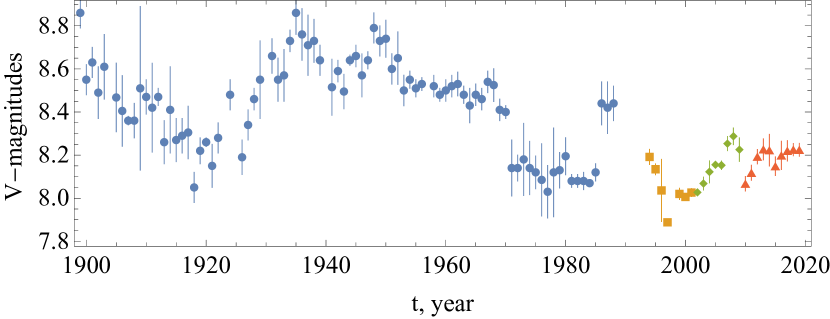
Figure 1: Long-term variations of the yearly-mean V-magnitudes of the star V833 Tau over 120 yr (1899-2019). The ordinate axis is digitized so that the minimal brightness of a star corresponds to the maximal activity (increasing of the starspot number). The data sets are compiled from the following sources: blue circles in the interval 1899-1988 – Hartmann et al. (1981) and Bondar’ (1995), yellow squares in the interval 1994-2001 – Alekseev & Bondar’ (1998) and Alekseev (2001), green rombs – ASAS data for 2002-2009, red triangles – KWS data for 2010-2919. Error bars show standard deviations.

4 Conservative approach for data interpretation

Our conservative approach for the interpretation of stellar activity data is based on applying the ideas and tools which pass all reliability tests analysing similar solar activity records (typically, some sorts of sunspot data). We consider the spectral properties of oscillations in the stellar spot tracer. We suppose that stellar dynamo produces the main cycle of activity which can be identified with a manifestation similar to the solar activity cycles. Analysis of the pronounced peaks in the integral spectrum is not sufficient for association with the 11-yr cycle in sunspot data. One needs to identify how its amplitude and shape are evolving in time. Wavelets, as a local form of the Fourier transform, seem to be a natural tool to get the time-frequency profile of any kinds of superposed oscillations. Certainly, this interpretation of the 1D signal deserves a confirmation, say, in form of a stellar butterfly diagram which should be compared with the solar ones. However this strict demand is mainly still out of the abilities of contemporary observations.

We note that wavelet spectra for some stars do not exhibit a pronounced peak (e.g. Frick et al., 1997). Our intention in this paper is to make one more step in this stellar-solar analogy. An instructive example is the so-called quasi-biennial oscillations; we bear in mind quasi-periodic oscillations in a mid-term range (i.e., ranging from 1 month to about 11 yr) which are emphasized in the 11-yr solar cycle at its activity maximum. However, taking into account the whole data record and evaluating statistical significance, we have found that quasi-biennial oscillations form a continuous spectrum of stochastic oscillations (Frick et al., 2020). This behavior reflects the turbulent nature of solar activity. Our wavelet analysis of a stellar activity tracer aims to recognize pronounced features that can be associated with the main cycle. Based on the interpretation of this similarity, we will do our best for now, considering what improvements can be expected given future observations. At least, we offer a conservative first step in this study.

4.1 Wavelet analysis

Spectral properties of the signal which change over time can be revealed with wavelet analysis. The continuous wavelet transform of the real signal $f(t)$ is defined as:

$$w_{\kappa}(\tau,t)={\tau}^{-\kappa}\int_{-\infty}^{\infty}f(t)\psi^{*}\left(\frac{t^{\prime}-t}{\tau}\right)dt^{\prime},$$ (1)

where $\psi(t)$ is the analysing wavelet, $\tau$ defines the scale (period of oscillation) and $t$ defines position in time. $\kappa$ is a free parameter which is chosen for the sake of convenience plotting the wavelet spectrogram (balancing structures at different scale). The signal can be restored using the inverse wavelet transform:

$$f(t)=\frac{1}{c_{\psi}}\int_{t_{\rm min}}^{t_{\rm max}}\int_{\tau_{\rm min}}^{\tau_{\rm max}}w_{\kappa}(\tau,t)\psi\left(\frac{t^{\prime}-t}{\tau}\right)\frac{d\tau\,dt^{\prime}}{{\tau}^{3-\kappa}},$$ (2)

where $t_{\rm min}$ and $t_{\rm max}$ determine the observational period. $\tau_{\rm min}$ and $\tau_{\rm max}$ are prescribed by the length and resolution of time series, theoretically in an ideal case $\tau\in(0,\infty)$. In practice, these limits can depend on time. Defining functions $\tau_{\rm min}(t)$ and $\tau_{\rm max}(t)$ allows one to restore the signal using a desired band of scales in the wavelet spectrogram. We use this option in the next section. The integral wavelet spectrum (kind of a smoothed version of the Fourier spectrum) is

$$S(\tau)=\int_{t_{\rm min}}^{t_{\rm max}}|w_{\kappa}(\tau,t^{\prime})|^{2}\frac{dt^{\prime}}{{\tau}^{3-2\kappa}}.$$ (3)

The appropriate resolution in time and scale can be provided using the popular Morlet wavelet: $\psi(t)=e^{-t^{2}}\left(e^{2\pi\imath t}-e^{-\pi^{2}}\right)$.

4.2 Solar activity analysis

We reproduce here the most important steps and argumentation of the following wavelet analysis by applying them to the sunspot area record. We choose a time interval 1876-2016 to be comparable in length to the V833 Tau data for comparison (see in Fig. 2). In principle, there are more long solar activity reconstructions (e.g. Usoskin et al., 2004) which are very interesting for understanding of solar activity, yet they seem to be excessive in the present context.

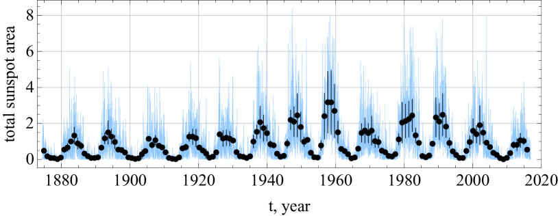
Figure 2: The total sunspot area as observed by the Royal Greenwich Observatory for the period 1874-1976 and extended to 2016 by the USAF/NOAA dataset (given in units of $10^{-9}$ of solar disk). Daily variation is shown by blue curve, and yearly mean and variance is shown by black dots with bars.

The wavelet spectrogram shown in Fig. 3 presents the intensity distribution of the wavelet coefficients $w_{1/2}(\tau,t)$, where the colour reflects the amplitude at the time $t$ and scale $\tau$. The most pronounced strip is seen at $\tau=11$ yr and corresponds to the nominal 11-yr Schwabe cycle. A particular wavy shape of this strip reveals amplitude and period modulations. In fact, the amplitude of the 11-yr cycle varies significantly but we do not see it because the peak values are clipped and presented in white. This allows us to show other details. The large scale (long periodicity) structure occurs at $\tau\approx 40$ and $t\approx 1980$. The small scale (like ’waterfall’) structures occur periodically at scales $\tau<11$ and around the activity phase of maximum sunspot areas.

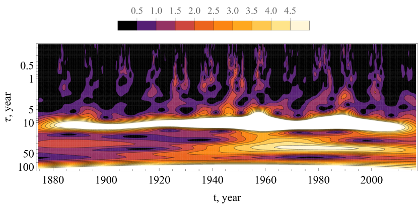
Figure 3: Wavelet spectrograms for the solar data (white area denotes clipped values $|w_{1/2}|$¿5)

The cumulative contribution of oscillation energy at different scales can be seen in the integral wavelet spectrum (Fig. 4). The solar activity’s 11-yr cycle is visible as a pronounced peak nearby $\tau=11$yr. The single structure at the longer period corresponds to a local maximum. The increase of $S(\tau)$ at $\tau=100$yr is related to the long-term variation known as the Gleissberg cycle (Gleissberg, 1965). Next, we focus on the mid-term range $\tau\in[0.1,5]$ (it is in a middle between 11-yr solar cycle and 1-month rotation period). The overall power spectral density follows a power law with a slope of about ${2/3}$. This means that the system exhibits stochastic behaviour under a turbulent regime. This conclusion can be made only on the basis of a sufficiently long observation of a dozen of the characteristic times of large-scale magnetic field evolution, in our case about 13 solar activity cycles. Studying individual shorter intervals, it will be difficult to confirm the interpretation of the local peaks at any particular short periods. One can see many of them in the individual spectra which were obtained for six individually separated 22-yr time spans (i.e., thin curves in Fig. 4).

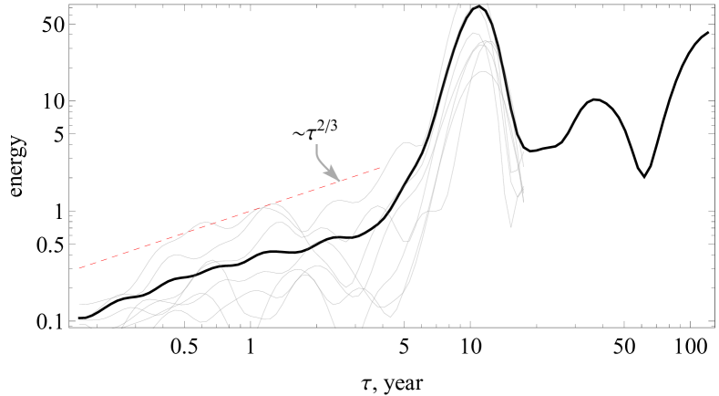
Figure 4: Solar activity spectra: integral wavelet spectrum for the whole data series (thick curve) and for subsequent 22-yr intervals (thin curves).

5 Wavelet analysis of the V833 Tau activity data

Let us consider how the proposed conservative approach would works when applied to V833 Tau. It looks plausible, just from the naked eye inspection of the wavelet spectrogram in Fig. 5, that V833 Tau demonstrates a rich variety of multi-scale oscillations. First of all, we do not see a bright strip that is in solar spectrogram (Fig. 3). With some care, one can distinguish a few structures between 10 and 40 yr (i.e., the interval where one suspects the star’s dynamo may act), which are slightly linked over time. The corresponding area is emphasised using two green lines in Fig. 5.

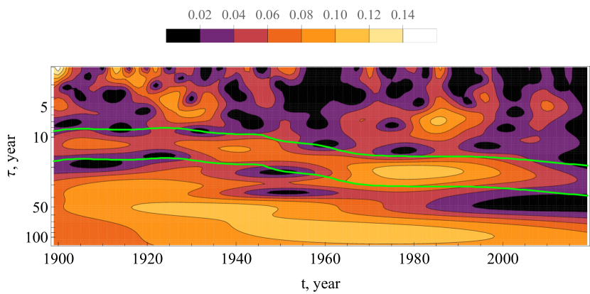
Figure 5: Wavelet spectrogram for the magnetic activity of V833 Tau ($|w_{1}|$). Green lines highlight the range of scales at which the continuous oscillation is traced for further reconstruction.

The integral wavelet spectrum for the V833 Tau data is shown in Fig. 6. On the one hand, we do not observe a local maximum which could be qualitatively compared with that for the solar spectrum (Fig. 4). There is a bump for $\tau$ between 30 and 40 yr which is a contribution of the isolated band to the spectrogram. We apply Monte-Carlo simulations using standard error given for each data point in order to evaluate the upper bound of the confidential interval at the level of 0.9. One can see that the maximum at $\tau=40$ yr is not sufficiently significant. On the other hand, the integral wavelet spectrum of V833 Tau in Fig. 6 can be described by a power law with $\tau^{3/2}$. The small scale part ($\tau\lesssim 10$) might be affected by noise but the rest seems statistically robust in sense that it is significant beyond observational noise. We recall again that a power-law scaling is expected for highly turbulent systems in the context of long observational records. If the statistics is still insufficient, the spectrum reveals an approximate power law relation, and the quality of approximation should improve as more data are available. We suppose that this has been confidently shown for solar data but it is illustrated here for V833 Tau.

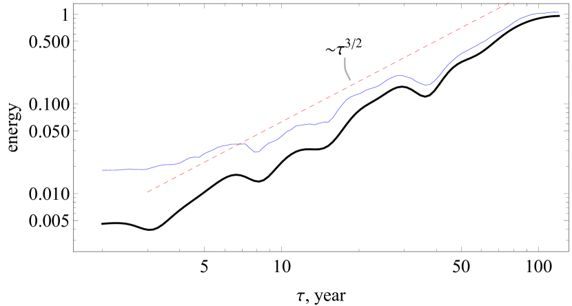
Figure 6: Integral wavelet spectrum for V833 Tau (black curve). Blue thin curve shows the upper boundary of 0.9 confidential interval.

We find that the V833 Tau spectrum follows a power-law function. This means structural self-similarity of the V833 Tau data that is more comparable to the mid-term oscillations of solar activity. Our conservative point of view necessarily leads to a conclusion that the V833 Tau activity cycle (expected to be similar to the solar cycle) is longer than a century, i.e., the timescale of V833 Tau intrinsic oscillation is an order of magnitude larger than that known for solar activity. This result means that observations for over about 1000 years would be needed to demonstrate cyclic behavior for V833 Tau. This statement can be illustrated by analysing the fragment of solar data which includes a couple of solar cycles only. According to this statement, we can try to see what we will observe when the solar records are shortened in length by 10 times. Let us examine the wavelet spectrogram for the time interval from 1924 to 1943 (Fig. 7). We may get an impression that something important is hiding behind the set of structures visible near $\tau=1$, or, even more important, behind the continuous strip along $\tau=5$. We propose that this impression would be deceptive.

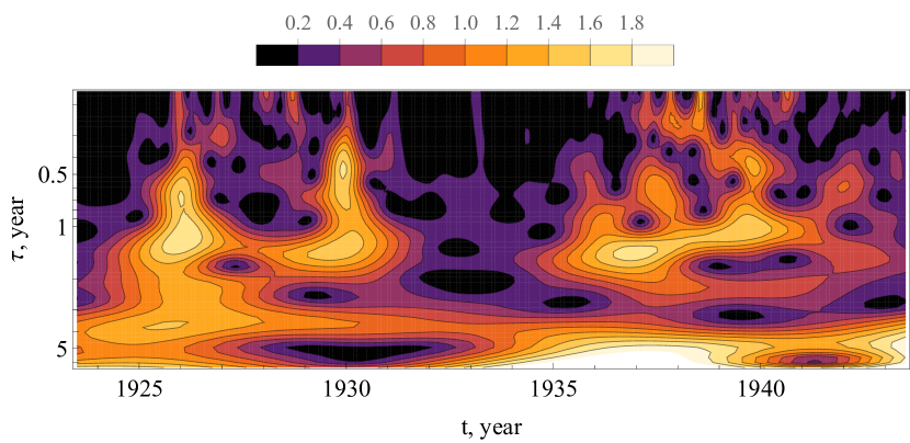
Figure 7: Enlarged fragment of the wavelet spectrogram shown in Fig. 3.

6 Discussion and conclusion

We conclude that the V833 Tau activity data for the 120 yr between 1899-2019 obeys the continuous spectrum of fluctuations without any significantly pronounced peaks. The activity spectrum reveals a power law behaviour in almost the whole range of available scales ($3<\tau<100$ yr) and this result is comparable with the behaviour of solar activity observed at scales $0.1<\tau<10$ yr. It seems natural to suppose that V833 Tau may have a cycle of about 80-100 yr however the available data are simply yet insufficient to isolate the proposed cycle. We tentatively and conservatively deduced that the physical timescale of the dynamo engine driving the activity in V833 Tau is about 10 times longer than that for solar dynamo.

The dynamo drivers underlying solar cycle in the framework of solar dynamo include such delicate characteristics of solar hydrodynamics as the degree of mirror asymmetry of solar convection and the meridional circulation. Contemporary astronomers made many important attempts to quantify these characteristics. However, it would be an exaggeration to say that our knowledge is sufficiently reliable in this respect, neglecting corresponding stellar properties. In principle, stellar dynamo models admit cycles much longer than the solar ones (e.g. Shulyak et al., 2015), whereas the shorter time scale are occupied by stochastic dynamics. The co-existing long and short stellar activity cycles can be modelled by studying the interplay of near-surface dynamo and a dynamo operating in deeper layers (Brandenburg et al., 2017). Analyses of the starspot rotational modulations in 1998 main-sequence stars observed by the Kepler satellite mission allowed one to recognize either long-living spots in activity complexes of stars with saturated magnetic dynamos or the spot emergence, which is modulated by large scale turbulent convection (Arkhypov et al., 2018).

We note that a dynamo can produce a steady magnetic field with more or less pronounced quasi-periodic fluctuations. Such magnetic configurations happen in spiral galaxies (e.g. Beck et al., 1996) or in the Earth (e.g. Gradstein et al., 2020). It is interesting that V833 Tau is both quite young and a very active star: its coronal radiation $L_{X}/L_{\rm bol}$ is close to 10^-3 and the rotation period is less than 2 days, i.e., it rotates more than 10 times faster than the Sun, which may saturate its activity (cf. Reiners et al., 2014). For a saturated mode of activity, stellar dynamo is expected to enhance a quasi-stationary magnetic field with chaotic variations, yet without a pronounced cycle (Baliunas et al., 1996). A regular cycle begins when the saturated regime of activity changes to the solar-type one, in which the activity level depends on the rotation period (Katsova et al., 2015). Nizamov et al. (2017) showed that the activity of late spectral-type K stars transitions to exhibiting regular cycles when its rotation period is equal to 3 days. It opens a possibility that V833 Tau, in its stellar evolutionary stage, still did not reach the stage to exhibit pronounced cyclic activity.

An alternative point of view suggests that a time series for V833 Tau is too short for any conclusive analysis of long-time variations ($\tau>50$ yr) and insists on a search for the particular oscillation in a range comparable with the Sun’s 11-yr cycle. Following this argument, we have tried to isolate the features dominating in the range of timescales below 50 yrs. We have made an attempt to restore the signal using certain wavelet coefficients corresponding to the dynamo wave for V833 Tau. Figure 8 presents two possible reconstructions, of which one is done using the wavelet coefficients in a fixed range of scales, i.e., $10<\tau<40$ yr (blue dashed curve), and the other is done in an adaptive band as a sort of a corridor. The latter is shown in Fig. 5 by green curves. At this stage, in both reconstructions, the bright structure centered in wavelet plane at $t\approx 1980,\tau\approx 20$ yr, and match pretty well. However, at the earlier interval, namely, for the period of $t\approx 1920-1930$ the blue dashed curve has a phase break, whereas the period of oscillations traced by the red curve is noticeably shortened (i.e., the blue curve missed one cycle against the red one; see Figure 8). Such a behavior observed in the V833 Tau record does not seemed to manifest itself in solar activity. In contrast, a detailed study of period duration and phase of the 11-yr solar oscillations may ultimately reveal a synchronized clock-like process within magnetically active layers in the Sun (Dicke, 1978).

Let us summarize our main conclusions. Wavelet analysis of the 120 yr long photometric variations for V833 Tau indicates that the long term variations of V833 Tau are similar to mid-term solar activity. If a stellar cycle for V833 Tau exists, then it is an order of magnitude longer than the solar one. However, we cannot completely exclude the scenario that V833 Tau has essentially an unstable dynamo and its cycle length varies within the period of 10 – 40 yr.

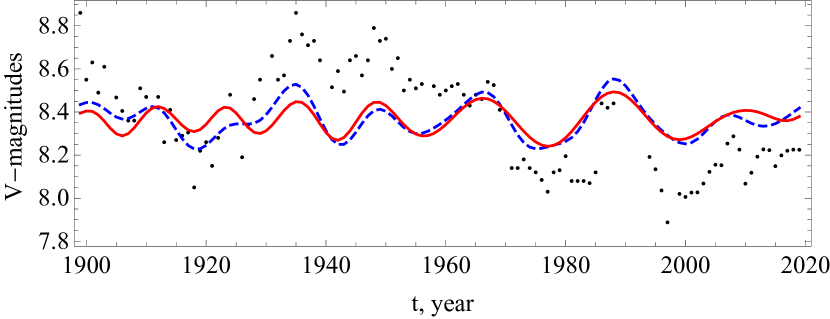
Figure 8: Restored signals from the wavelet coefficients corresponding to the most pronounced spectral feature in V833 Tau data: the reconstruction along the vicinity of local maximum marked by green lines in Fig. 5 (red curve), and the reconstruction in the fixed scale range $10<\tau<40$ yr (blue dashed curve). Original data are shown by black points.

References

- Alekseev (2001) Alekseev I. Y., 2001, Spotted low mass stars. Astroprint, Odessa
- Alekseev (2005) Alekseev I. Y., 2005, Astrophysics, 48, 20
- Alekseev & Bondar’ (1998) Alekseev I. Y., Bondar’ N. I., 1998, Astron. Rep., 42, 655
- Alekseev & Gershberg (1997) Alekseev I. Y., Gershberg R. E., 1997, Astron. Rep., 41, 207
- Arkhypov et al. (2018) Arkhypov O. V., Khodachenko M. L., Lammer H., Güdel M., Lüftinger T., Johnstone C. P., 2018, MNRAS, 473, L84
- Auvergne et al. (2009) Auvergne M., et al., 2009, A&A, 506, 411
- Baliunas et al. (1995) Baliunas S. L., et al., 1995, ApJ, 438, 269
- Baliunas et al. (1996) Baliunas S. L., Nesme-Ribes E., Sokoloff D., Soon W. H., 1996, ApJ, 460, 848
- Beck et al. (1996) Beck R., Brandenburg A., Moss D., Shukurov A., Sokoloff D., 1996, ARA&A, 34, 155
- Bondar’ (1995) Bondar’ N. I., 1995, A&AS, 111, 259
- Bondar’ (2015) Bondar’ N. I., 2015, Astron. Rep., 59, 221
- Bondar’ (2017) Bondar’ N. I., 2017, Astron. Rep., 61, 130
- Bondar’ et al. (2019) Bondar’ N. I., Gorbunov M. A., Shlyapnikov A. A., 2019, A Search for Cyclic Activity of Red Dwarfs Using Photometric Surveys. p. 180
- Bopp et al. (1981) Bopp B. W., Noah P. V., Klimke A., Africano J., 1981, ApJ, 249, 210
- Borucki et al. (2010) Borucki W. J., et al., 2010, Science, 327, 977
- Brandenburg et al. (2017) Brandenburg A., Mathur S., Metcalfe T. S., 2017, ApJ, 845, 79
- Dicke (1978) Dicke R. H., 1978, Nature, 276, 676
- Doyle et al. (2018) Doyle J. G., et al., 2018, MNRAS, 475, 2842
- Eggen & Sandage (1965) Eggen O. J., Sandage A. R., 1965, ApJ, 141, 821
- Frick et al. (1997) Frick P., Baliunas S. L., Galyagin D., Sokoloff D., Soon W., 1997, ApJ, 483, 426
- Frick et al. (2004) Frick P., Soon W., Popova E., Baliunas S., 2004, New Astron., 9, 599
- Frick et al. (2020) Frick P., Sokoloff D., Stepanov R., Pipin V., Usoskin I., 2020, MNRAS, 491, 5572
- Gleissberg (1965) Gleissberg W., 1965, J. Brit. Astr. Assoc., 75, 227
- Gliese & Jahreiß (1991) Gliese W., Jahreiß H., 1991, Preliminary Version of the Third Catalogue of Nearby Stars, On: The Astronomical Data Center CD-ROM: Selected Astronomical Catalogs
- Gradstein et al. (2020) Gradstein F., Ogg J. G., Schmitz M., Ogg G., 2020, Geologic Time Scale 2020. Elsevier
- Griffin et al. (1985) Griffin R. F., Gunn J. E., Zimmerman B. A., Griffin R. E. M., 1985, AJ, 90, 609
- Grundahl et al. (2008) Grundahl F., Christensen-Dalsgaard J., Kjeldsen H., Frandsen S., Arentoft T., Kjaergaard P., Jørgensen U. G., 2008, in Deng L., Chan K. L., eds, IAU Symposium Vol. 252, The Art of Modeling Stars in the 21st Century. pp 465–466, doi:10.1017/S174392130802351X
- Halbwachs et al. (2000) Halbwachs J.-L., Arenou F., Mayor M., Udry S., 2000, in Reipurth B., Zinnecker H., eds, IAU Symposium Vol. 200, Birth and evolution of binary stars. p. 132
- Halbwachs et al. (2018) Halbwachs J. L., Mayor M., Udry S., 2018, A&A, 619, A81
- Hall & Lockwood (1995) Hall J. C., Lockwood G. W., 1995, ApJ, 438, 404
- Hall et al. (2009) Hall J. C., Henry G. W., Lockwood G. W., Skiff B. A., Saar S. H., 2009, AJ, 138, 312
- Hartmann et al. (1981) Hartmann L., Bopp B. W., Dussault M., Noah P. V., Klimke A., 1981, ApJ, 249, 662
- Hathaway (2015) Hathaway D. H., 2015, Liv. Rev. Solar Phys., 12, 4
- Heintz (1981) Heintz W. D., 1981, ApJS, 46, 247
- Karak et al. (2020) Karak B. B., Tomar A., Vashishth V., 2020, MNRAS, 491, 3155
- Karoff et al. (2019) Karoff C., Metcalfe T. S., Montet B. T., Jannsen N. E., Santos A. R. G., Nielsen M. B., Chaplin W. J., 2019, MNRAS, 485, 5096
- Katsova et al. (2015) Katsova M. M., Bondar N. I., Livshits M. A., 2015, Astron. Rep., 59, 726
- Kiefer et al. (2017) Kiefer R., Schad A., Davies G., Roth M., 2017, A&A, 598, A77
- Kiefer et al. (2019) Kiefer R., Broomhall A.-M., Ball W. H., 2019, Front. Astron. Space Sci., 6, 52
- Lehmann et al. (2018) Lehmann L. T., Jardine M. M., Mackay D. H., Vidotto A. A., 2018, MNRAS, 478, 4390
- Lockwood et al. (1997) Lockwood G. W., Skiff B. A., Radick R. R., 1997, ApJ, 485, 789
- Lucas & Roche (2002) Lucas P. W., Roche P. F., 2002, MNRAS, 336, 637
- Montet et al. (2017) Montet B. T., Tovar G., Foreman-Mackey D., 2017, ApJ, 851, 116
- Moss & Sokoloff (2007) Moss D., Sokoloff D., 2007, MNRAS, 377, 1597
- Moss et al. (2011) Moss D., Sokoloff D., Lanza A. F., 2011, A&A, 531, A43
- Nizamov et al. (2017) Nizamov B. A., Katsova M. M., Livshits M. A., 2017, Astronomy Letters, 43, 202
- Olah & Pettersen (1991) Olah K., Pettersen B. R., 1991, A&A, 242, 443
- Oláh et al. (2001) Oláh K., Strassmeier K. G., Kovári Z., Guinan E. F., 2001, A&A, 372, 119
- Oláh et al. (2016) Oláh K., Kővári Z., Petrovay K., Soon W., Baliunas S., Kolláth Z., Vida K., 2016, A&A, 590, A133
- Oswalt et al. (1988) Oswalt T. D., Hintzen P. M., Luyten W. J., 1988, ApJS, 66, 391
- Parker (1955) Parker E. N., 1955, ApJ, 122, 293
- Pettersen (1989) Pettersen B. R., 1989, A&A, 209, 279
- Pojmanski (1997) Pojmanski G., 1997, Acta Astron., 47, 467
- Radick et al. (1998) Radick R. R., Lockwood G. W., Skiff B. A., Baliunas S. L., 1998, ApJS, 118, 239
- Radick et al. (2018) Radick R. R., Lockwood G. W., Henry G. W., Hall J. C., Pevtsov A. A., 2018, ApJ, 855, 75
- Reiners et al. (2014) Reiners A., Schüssler M., Passegger V. M., 2014, ApJ, 794, 144
- Salabert et al. (2016) Salabert D., et al., 2016, A&A, 596, A31
- Scholz et al. (2018) Scholz R. D., Meusinger H., Jahreiß H., 2018, A&A, 613, A26
- Schrijver & Zwaan (2008) Schrijver C. J., Zwaan C., 2008, Solar and Stellar Magnetic Activity. Cambridge University Press
- Shulyak et al. (2015) Shulyak D., Sokoloff D., Kitchatinov L., Moss D., 2015, MNRAS, 449, 3471
- Strassmeier et al. (1993) Strassmeier K. G., Hall D. S., Fekel F. C., Scheck M., 1993, A&AS, 100, 173
- Testa et al. (2015) Testa P., Saar S. H., Drake J. J., 2015, Phil. Trans. R. Soc. A, 373, 20140259
- Usoskin et al. (2004) Usoskin I. G., Mursula K., Solanki S., Schüssler M., Alanko K., 2004, A&A, 413, 745
- Vida et al. (2016) Vida K., et al., 2016, A&A, 590, A11
- Vidotto et al. (2014) Vidotto A. A., et al., 2014, MNRAS, 441, 2361
- Viviani et al. (2018) Viviani M., Warnecke J., Käpylä M. J., Käpylä P. J., Olspert N., Cole-Kodikara E. M., Lehtinen J. J., Brandenburg A., 2018, A&A, 616, A160
- Walker et al. (2003) Walker G., et al., 2003, PASP, 115, 1023