A distribution free test for changes in the trend function of locally stationary processes

Abstract.

In the common time series model $X_{i,n}=\mu(i/n)+\varepsilon_{i,n}$ with non-stationary errors we consider the problem of detecting a significant deviation of the mean function $\mu$ from a benchmark $g(\mu)$ (such as the initial value $\mu(0)$ or the average trend $\int_{0}^{1}\mu(t)dt$). The problem is motivated by a more realistic modelling of change point analysis, where one is interested in identifying relevant deviations in a smoothly varying sequence of means $(\mu(i/n))_{i=1,\ldots,n}$ and cannot assume that the sequence is piecewise constant. A test for this type of hypotheses is developed using an appropriate estimator for the integrated squared deviation of the mean function and the threshold. By a new concept of self-normalization adapted to non-stationary processes an asymptotically pivotal test for the hypothesis of a relevant deviation is constructed. The results are illustrated by means of a simulation study and a data example.

Key words: change point analysis, local stationary processes, nonparametric regression

1. Introduction

Within the last decades, the detection of structural breaks in time series has become a very active area of research with many applications in fields like climatology, economics, engineering, genomics, hydrology, etc. (see Aue and Horváth, 2013; Jandhyala et al., 2013; Woodall and Montgomery, 2014; Sharma et al., 2016; Chakraborti and Graham, 2019; Truong et al., 2020, among many others). In the simplest case, one is interested in detecting structural breaks in the sequence of means $(\mu_{i})_{i=1,\dots,n}=(\mu(i/n))_{n\in\mathbb{N}}$ of a time series $(X_{i,n})_{i=1,\dots,n}$ corresponding to a location model of the form

$$X_{i,n}=\mu(i/n)+{\varepsilon}_{i,n}~{},~{}~{}i=1,\ldots,n~{}.$$ (1.1)

A large part of the literature considers the problem of detecting changes in a piecewise constant mean function $\mu:[0,1]\to\mathbb{R}$, where early references assume the existence of at most one change point (see, e. g. Priestley and Subba Rao, 1969; Wolfe and Schechtman, 1984; Horváth et al., 1999, among others) and more recent literature investigates multiple change points (see, e.g. Frick et al., 2014; Fryzlewicz, 2018; Dette et al., 2020; Baranowski et al., 2019, among many others). The errors $({\varepsilon}_{i,n})_{i=1,\dots,n}$ in model (1.1) are usually assumed to form at least a stationary process and many theoretical results for detecting multiple change points are only available for independent identically distributed error processes. These assumptions simplify the statistical analysis of structural breaks substantially, as - after removing the piecewise constant trend - one can work under the assumption of a stationary or an independent identically distributed error process and smoothing is not necessary to estimate the trend function.

On the other hand, the assumption of a strictly piecewise constant mean function might not be realistic in many situations and it might be more reasonable to assume that $\mu$ varies smoothly rather than abrupt. A typical example is temperature data (see, e. g. Karl et al., 1995; Collins et al., 2000) where it might be of more interest to investigate whether the mean function deviates fundamentally from a given benchmark denoted by $g(\mu)$. Here $g$ is a functional of the mean function, such as the value at the point $0$, that is $g(\mu)=\mu(0),$ or an average over a certain time period, that is

$$g(\mu)=\frac{1}{t_{1}-t_{0}}\int_{t_{0}}^{t_{1}}\mu(x)dx~{}~{}\text{ for some }~{}~{}0\leq t_{0}<t_{1}\leq 1$$ (1.2)

(see Section 2 for more details). Moreover, there also exist many time series exhibiting a non-stationary behaviour in the higher order moments and dependence structure (see Stărică and Granger, 2005; Elsner et al., 2008; Guillaumin et al., 2017, among others), and the detection of fundamental deviations from a benchmark in a sequence of gradually changing means under the assumption of a location model with a stationary error process might be misleading.

In this paper we propose a distribution free test for relevant deviations of the mean function $\mu$ from a given benchmark $g(\mu)$ in a location scale model of the form (1.1) with a non-stationary error process. More precisely, for some pre-specified threshold $\Delta>0$ we are interested in testing the hypotheses

$$H_{0}:d_{0}=\Big{(}\int_{0}^{1}\big{(}\mu(x)-g(\mu)\big{)}^{2}\tau({\mathrm{d}}x)\Big{)}^{1/2}\leq\Delta\quad\text{vs.}\quad H_{1}:d_{0}>\Delta,$$ (1.3)

where $\tau$ is an appropriate measure on the interval $[0,1]$ chosen by the statistician. This means that we are looking for “substantial” deviations of the mean function from a given benchmark $g(\mu)$ in an $L^{2}$-sense. The choice of the threshold depends on the particular application and is related to a balance between bias and variance as the detection of deviations from a (constant) mean often results in an adaptation of the statistical analysis (for example in forecasting). As such an analysis is performed “locally”, resulting estimators will have a smaller bias but a larger variance. However, if the changes in the signal are only weak, such an adaptation might not be necessary because a potential decrease in bias might be overcompensated by an increase of variance.

In principle, a test for the hypotheses in (1.3) could be developed using a nonparametric estimate of the mean function $\mu$ to obtain an estimate, say $\hat{d}_{0}$, of the distance $d_{0}$. The null hypothesis in (1.3) is then rejected for large values of $\hat{d}_{0}$. However, the distribution of the test statistic will depend in an intricate way on the dependence structure of the non-stationary error process in model (1.1), which is difficult to estimate. To address this problem we will introduce a new concept of self-normalization and construct an (asymptotically) pivotal test statistic for the hypotheses in (1.3). The basic idea of our approach is to permute the data and consider the partial sum process of this permutation, thus, taking into account observations over the whole interval rather than only the first observations. The new concept and the asymptotic properties of the standardized statistic can be found in Section 3, while some details on the testing problem and mathematical background on locally stationary processes are introduced in Section 2. In Section 4 we investigate the finite sample properties of the proposed testing procedure by means of a simulation study and provide an application to temperature data. Finally, in Section A, the proofs of the theoretical results in Section 3 are presented.

1.1. Related literature

Despite of its importance the problem of detecting relevant deviations in a sequence of gradually changing means has only been considered by a few authors. Dette and Wu (2019) investigate a mass excess approach for this problem. More precisely, these authors measure deviations from the benchmark by the Lebesgue measure of the set $\{t\in[0,1]:|\mu(t)-g(\mu)|>\Delta\}$ and test whether this quantity exceeds a certain threshold $c>0$. Their approach requires estimation of the local long-run variance and multiplier bootstrap. More recently, Bücher et al. (2020) propose the maximal distance to measure relevant deviations from the benchmark and consider the null hypothesis $H_{0}:\sup_{t\in[0,1]}|\mu(t)-g(\mu)|\leq\Delta$. While the maximum deviation might be easy to interpret for practitioners, the asymptotic analysis of a corresponding estimate is challenging. In particular it requires an estimation of the long-run variance and additionally the estimation of the sets, where the absolute difference $|\mu(t)-g(\mu)|$ attains its sup-norm. The methodology proposed here avoids the problem of estimating tuning parameters of this type using an $L^{2}$-norm in combination with a new concept of self-normalization.

Ratio statistics or self-normalization have been introduced by Horváth et al. (2008) and Shao (2010) in the context of change point detection in stationary processes and avoid a direct estimation of the long-run variance through a convenient rescaling of the test statistic. The currently available self-normalization procedures are based on partial sum processes (see Shao, 2015, for a recent review), which usually (under the assumption of stationarity) have a limiting process of the form $\{\sigma W(\lambda)\}_{\lambda\in[0,1]}$, where $\{W(\lambda)\}_{\lambda\in[0,1]}$ is a known stochastic process and $\sigma$ an unknown factor encapsulating the dependency structure of the underlying process. In this case the factorisation of the limit into the long-run variance and a probabilistic term is used to construct a pivotal test statistic by forming a ratio such that the factor $\sigma$ in the numerator and denominator cancels. However, in the case of non-stationarity, the situation is more complicated, because the limiting process is of the form $\big{\{}\int_{0}^{\lambda}\sigma(u){\mathrm{d}}W(u)\big{\}}_{\lambda\in[0,1]}$ such that the probabilistic and the part representing the dependence structure cannot be separated. Zhao and Li (2013) and Rho and Shao (2015) discuss in fact these problems in the context of locally stationary time series, but the proposed self-normalizations need to be combined with a wild bootstrap. In this paper, we present a full self-normalization procedure for non-stationary time series, which might be also useful for testing classical hypotheses.

2. The testing problems and mathematical Preliminaries

Throughout this paper $\mathcal{L}^{2}([0,1])$ denotes the space of real-valued square-integrable functions on $[0,1]$ and $L^{2}([0,1])$ the corresponding normed vector space of equivalence classes. Let $\langle f,g\rangle=\int_{0}^{1}f(x)g(x){\mathrm{d}}x$ denote the scalar product in $L^{2}([0,1])$ and $\|f\|_{2}=\langle f,f\rangle^{1/2}$ the corresponding norm, for $f,g\in L^{2}([0,1])$. Further, $\langle f,g\rangle_{\tau}=\int_{0}^{1}f(x)g(x)\tau({\mathrm{d}}x)$ and $\|f\|_{2,\tau}=\langle f,f\rangle_{\tau}^{1/2}$, for $f,g\in L^{2}([0,1],\tau)$. Finally, for the sake of readability, for functions in $\mathcal{L}^{2}([0,1])$, we denote the integral $\int_{0}^{1}f(x)g(x){\mathrm{d}}x$ by $\langle f,g\rangle$. Finally, if $X$ is a real-valued random variable we use the notation (in the case of existence) $\|X\|_{q,\Omega}=\big{(}\mathbb{E}[|X|^{q}]\big{)}^{1/q}$, for $q\geq 1$.

2.1. Relevant deviations in a sequence of gradually changing means

Recall the definition of model (1.1) and the hypotheses (1.3). Different benchmarks may be of interest in applications. For example, if one is interested in deviations from the value of the mean function at a given time, say $t\in[0,1]$, one could choose $g(\mu)=\mu(t)$, while relevant deviations from an average over a certain time period are obtained for the choice (1.2). In particular if $t_{0}$, $t_{1}$ and $\tau$ are chosen $0$, $1$ and the Lebesgue measure, respectively, one compares the local mean $\mu(x)$ with the overall mean $g(\mu)=\bar{\mu}=\int_{0}^{1}\mu(y){\mathrm{d}}y$ and the hypotheses in (1.3) read as follows

$$H_{0}:\Big{(}\int_{0}^{1}\big{(}\mu(x)-\bar{\mu}\big{)}^{2}{\mathrm{d}}x\Big{)}^{1/2}\leq\Delta~{}\quad\text{vs.}\quad\Big{(}\int_{0}^{1}\big{(}\mu(x)-\bar{\mu}\big{)}^{2}{\mathrm{d}}x\Big{)}^{1/2}>\Delta.$$

The tests which will be developed in this paper are based on an appropriate estimate of the quantity

$$d_{0}=\Big{(}\int_{0}^{1}\big{(}\mu(x)-g(\mu)\big{)}^{2}\tau({\mathrm{d}}x)\Big{)}^{1/2}$$ (2.1)

for which we require precise estimates of the mean function $\mu$ and the threshold $g(\mu)$. Note that the measure $\tau$ in (2.1) is chosen by the statistician and therefore known.

Throughout this paper, we assume that $\tau$ is absolutely continuous with respect to the Lebesgue measure and has a piecewise continuous density, say $f_{\tau}$. Further, we assume that the mean function $\mu$ is sufficiently smooth, as specified in the following assumption.

Assumption 2.1.

The function $\mu:[0,1]\to\mathbb{R}$ is twice differentiable with Lipschitz continuous second derivative. In particular, this implies that the integrals $\int_{0}^{1}\mu^{2}(x){\mathrm{d}}x$ and $\int_{0}^{1}\mu^{2}(x)\tau({\mathrm{d}}x)$ are finite, thus, $\mu\in\mathcal{L}^{2}([0,1])$ and $\mu\in\mathcal{L}^{2}([0,1],\tau)$.

A natural idea for the construction of a test of the hypotheses (1.3) is to estimate the $L^{2}$-distance $d_{0}$ as defined in (2.1) and to reject the null hypothesis for large values of the corresponding estimate. For this purpose one can use the local linear estimator, which is defined as the first coordinate of the vector

$$\big{(}\hat{\mu}_{h_{n}}(t),\widehat{\mu^{\prime}}_{h_{n}}(t)\big{)}=\underset{b_{0},b_{1}}{\textnormal{argmin}}\sum_{i=1}^{n}\big{(}X_{i,n}-b_{0}-b_{1}(i/n-t)\big{)}^{2}K_{h_{n}}(i/n-t),$$ (2.2)

to estimate the mean function $\mu$ locally (see, for example Fan and Gijbels, 1996). In order to reduce the bias we consider the Jackknife estimator

$$\check{\mu}_{h_{n}}(t)=2\hat{\mu}_{h_{n}/\sqrt{2}}(t)-\hat{\mu}_{h_{n}}(t)$$ (2.3)

as proposed by Schucany and Sommers (1977) and obtain an estimate $\check{g}_{n}=g(\hat{\mu}_{h_{n}})$ of the threshold $g(\mu)$ (other estimates could be used as well). Here $h_{n}$ is a positive bandwidth satisfying $h_{n}=o(1)$ as $n\to\infty$, $K_{h}(\cdot)=K(\frac{\cdot}{h})$ and $K$ denotes a kernel function satisfying the following assumption.

Assumption 2.2.

The kernel $K$ is non-negative, symmetric, supported on the interval $[-1,1]$. It is twice differentiable, satisfies $\int_{[-1,1]}K(x)dx=1$ and Lipschitz continuous in an open interval containing the interval $[-1,1]$.

The estimate of $d_{0}$ can then be defined as

$$\|\check{\mu}_{h_{n}}-\check{g}_{n}\|_{2,\tau}=\Big{(}\int_{0}^{1}\big{(}\check{\mu}_{h_{n}}(x)-\check{g}_{n}\big{)}^{2}\tau({\mathrm{d}}x)\Big{)}^{1/2}~{}.$$ (2.4)

To study the asymptotic properties of the statistic defined in (2.4) and alternative estimates proposed in this paper (see Section 3 for more details) we require several assumptions regarding the dependency structure of the error process in model (1.1), which will be discussed next.

2.2. Locally stationary processes

For the proofs of our main results we require several assumption on the dependence structure of the non-stationary time series defined in (1.1). In the following, we work with the notion of local stationarity as introduced by Zhou and Wu (2009). To be precise, let $\eta=(\eta_{i})_{i\in\mathbb{Z}}$ be a sequence of independent identically distributed random variables and let $(\eta^{\prime})=(\eta_{i}^{\prime})_{i\in\mathbb{Z}}$ be an independent copy of $\eta$. Further, define $\mathcal{F}_{i}=\{\eta_{k}:k\leq i\}$ and $\mathcal{F}_{i}^{*}=(\ldots,\eta_{-2},\eta_{-1},\eta_{0}^{\prime},\eta_{1},\ldots,\eta_{i})$. Let $G:[0,1]\times\mathbb{R}^{\infty}\to\mathbb{R}$ denote a filter, such that $G(t,\mathcal{F}_{i})$ is a properly defined random variable for all $t\in[0,1]$.

A triangular array $\{({\varepsilon}_{i,n})_{1\leq i\leq n}\}_{n\in\mathbb{N}}$ is called locally stationary, if there exists a filter $G$, which is continuous in its first argument, such that

$${\varepsilon}_{i,n}=G(i/n,\mathcal{F}_{i})$$

for all $i\in\{1,\ldots,n\},n\in\mathbb{N}$. The physical dependence measure of a filter $G$ with $\sup_{t\in[0,1]}\|G(t,\mathcal{F}_{i})\|_{q,\Omega}<\infty$ with respect to $\|\cdot\|_{q,\Omega}$ is defined by

$$\delta_{q}(G,i)=\sup_{t\in[0,1]}\|G(t,\mathcal{F}_{i})-G(t,\mathcal{F}_{i}^{*})\|_{q,\Omega}.$$

A filter $G$ is called Lipschitz continuous with respect to $\|\cdot\|_{q,\Omega}$, if

$$\sup_{0\leq s<t\leq 1}\|G(t,\mathcal{F}_{i})-G(s,\mathcal{F}_{i})\|_{q,\Omega}/|t-s|<\infty.$$

The filter $G$ models the non-stationarity of $({\varepsilon}_{i,n})$. The quantity $\delta_{q}(G,i)$ measures the dependence of $({\varepsilon}_{i,n})$ and plays a similar role as mixing coefficients. We now state some assumptions regarding the error terms in model (1.1).

Assumption 2.3.

Let the triangular array $\{({\varepsilon}_{i,n})_{1\leq i\leq n}\}_{n\in\mathbb{N}}$ in (1.1) be centered and locally stationary with filter $G$, such that the following conditions are satisfied:

1. There exists a constant $\gamma\in(0,1)$ such that $\delta_{4}(G,i)=\mathcal{O}(\gamma^{i})$, as $i\to\infty$.

2. The filter $G$ is Lipschitz continuous with respect to $\|\cdot\|_{4,\Omega}$ and

   $$\sup_{t\in[0,1]}\|G(t,\mathcal{F}_{0})\|_{4,\Omega}<\infty.$$

3. The (local) long-run variance of $G$, defined as

   $$\sigma^{2}(t)=\sum_{i=-\infty}^{\infty}\textnormal{Cov}\big{(}G(t,\mathcal{F}_{i}),G(t,\mathcal{F}_{0})\big{)},$$ (2.5)

   for $t\in[0,1]$, is Lipschitz continuous and bounded away from zero, i. e.,

   $$\inf_{t\in[0,1]}\sigma^{2}(t)>0.$$

4. The moments of order $8$ are uniformly bounded, i. e., $\max_{1\leq i\leq n}\mathbb{E}{\varepsilon}_{i,n}^{8}<\infty$.

2.3. Testing for relevant differences - the problem of estimating the variance

Continuing the discussion in Section 2.1 it follows from the results given in Section 3 that the estimator (2.4) is asymptotically normal distributed if Assumptions 2.1, 2.2, 2.3 and an additional assumption on the consistency of the statistic $\check{g}_{n}$ are satisfied. More precisely, it can be shown (see Remark 3.7) that

$$\sqrt{n}\big{(}\|\check{\mu}_{h_{n}}-\check{g}_{n}\|_{2,\tau}^{2}-\|\mu-g(\mu)\|_{2,\tau}^{2}\big{)}\rightsquigarrow\mathcal{N}\big{(}0,4\|d_{\omega}\sigma\|_{2}^{2}\big{)},$$ (2.6)

where the symbol $\rightsquigarrow$ denotes weak convergence, $\sigma^{2}(\cdot)$ is the local long-run variance defined in (2.5) and $d_{\omega}(\cdot)$ denotes an unknown function, that depends on the function $\mu$ and the error process. In principle, if $\hat{\sigma}_{n}^{2}$ and $\hat{d}_{\omega}^{2}$ are estimators of the local long-run variance and the function $d_{\omega}$, respectively, a reasonable strategy would be to reject the null hypothesis in (1.3) if

$$\|\check{\mu}_{h_{n}}-\check{g}_{n}\|_{2,\tau}^{2}>\Delta^{2}+z_{1-\alpha}\frac{2\|\hat{d}_{\omega}\hat{\sigma}_{n}\|_{2}}{\sqrt{n}},$$ (2.7)

where $z_{1-\alpha}$ denotes the $(1-\alpha)$-quantile of the standard normal distribution. It will be shown in Remark 3.7 below, that this decision rule provides a consistent and asymptotic level $\alpha$-test for the hypotheses in (1.3). However, it turns out that this decision rule does not provide a stable test because local estimators of the long-run variance have a rather large variability.

In order to avoid the intricate estimation of the local long-run variance we will re-define the local linear estimator in (2.2) permuting the data and consider the partial sum process of the new estimators in the following section. This approach will enable us to construct an (asymptotically) pivotal test statistic for the hypotheses in (1.3).

3. A pivotal test statistic

3.1. Self-normalization

A common technique to avoid estimating the long-run variance are ratio statistics or self-normalization as first introduced by Horváth et al. (2008) and Shao (2010), which are based on a convenient rescaling of the test statistic. However, these concepts are not easy to transfer to non-stationary time series as they rely on the asymptotic properties of a corresponding partial sum process. To illustrate the problems of these concepts in non-stationary time series consider the simplest case of model (1.1), where the mean function is constant and the error process is stationary. In this case the estimate of the constant mean function $\mu$ from the partial sample $X_{1,n},\ldots,X_{\lfloor\lambda n\rfloor,n}$ is its mean and under the assumptions stated in Section 2 we have the weak convergence

$$\{B_{n}(\lambda)\}_{\lambda\in[0,1]}=\Big{\{}n^{-1/2}\sum_{i=1}^{\lfloor\lambda n\rfloor}\big{(}X_{i,n}-\mu\big{)}\Big{\}}_{\lambda\in[0,1]}\rightsquigarrow\{\sigma W(\lambda)\}_{\lambda\in[0,1]},$$

where $\big{\{}W(\lambda)\big{\}}_{\lambda\in[0,1]}$ denotes a standard Brownian motion and the long-run variance $\sigma^{2}$ is defined in (2.5) and does not depend on $t$ (because of the stationarity assumption). In this case, the factorisation of the limit into the long-run variance and a probabilistic term is used to construct a test statistic in the form of a ratio, such that $\sigma$ occurs in the nominator and denominator, and therefore cancels out. On the other hand, if the error process in model (1.1) is non-stationary (but the mean function is still constant) we have the weak convergence

$$\{B_{n}(\lambda)\}_{\lambda\in[0,1]}\rightsquigarrow\Big{\{}\int_{0}^{\lambda}\sigma(u){\mathrm{d}}W(u)\big{\}}_{\lambda\in[0,1]}.$$

In this case, the limiting distribution does not factorise and it is no longer possible to use the common self-normalization approach. Zhao and Li (2013) and Rho and Shao (2015) discuss locally stationary time series, but the proposed self-normalization procedures have to be combined with a wild bootstrap.

In this work, we present an alternative self-normalization procedure for non-stationary time series which does not require resampling to obtain (asymptotically) pivotal statistics. Our approach is based on the idea that in a locally stationary setting, observations from the whole interval $[0,1]$ need to be taken into account. Therefore, let $b_{n}$ denote a sequence with $b_{n}\to\infty$ and $b_{n}/n\to 0$, as $n\to\infty$, and let $\ell_{n}=\lfloor n/b_{n}\rfloor$. We define a (fixed) permutation of the set $\{1,\dots,n\}$ by

$$T:\left\{\begin{array}[]{ccl}\{1,\dots,n\}&\to&\{1,\dots,n\}\\ k&\mapsto&T_{k}=\left\{\begin{array}[]{rl}(k-1\mod\ell_{n})b_{n}+\lceil k/\ell_{n}\rceil,&\text{if}~{}k\leq\ell_{n}b_{n}\\ k,&\text{if}~{}k>\ell_{n}b_{n}\end{array}\right.\end{array}\right.$$

Note that for $k=i\ell_{n}+j$ it holds $T_{k}=(j-1)b_{n}+i+1$, where $i\in\{0,\dots,b_{n}\}$ and $j\in\{1,\dots,\ell_{n}\}$.

Roughly speaking, the mapping $T$ splits the set $\{1,\dots,n\}$ into $\ell_{n}$ blocks with block length $b_{n}$, that is

$$\{T_{1},\ldots,T_{\ell_{n}}\} = \{1,b_{n}+1,2b_{n}+1,\ldots,(l_{n}-1)b_{n}+1\}$$

$$\{T_{\ell_{n}+1},\ldots,T_{2\ell_{n}}\} = \{2,b_{n}+2,2b_{n}+2,\ldots,(l_{n}-1)b_{n}+2\}$$

$$\{T_{2\ell_{n}+1},\ldots,T_{3\ell_{n}}\} = \{3,b_{n}+3,2b_{n}+2,\ldots,(l_{n}-1)b_{n}+3\}$$

$$\quad\vdots\quad\quad\quad \vdots \quad\quad\quad\quad\quad\quad\quad\quad\quad\vdots$$

where the blocks correspond to the columns in the above display.

With this notation, for $\zeta>0$ and $\lambda\in[\zeta,1]$, we define the sequential local linear estimator of the mean function $\mu$ from the sample $X_{T_{1},n},\ldots,X_{T_{\lfloor\lambda n\rfloor},n}$ as the first coordinate of the vector

$$\big{(}\hat{\mu}_{h_{n}}(\lambda,t),\widehat{\mu^{\prime}}_{h_{n}}(\lambda,t)\big{)}=\underset{b_{0},b_{1}}{\textnormal{argmin}}\sum_{i=1}^{\lfloor\lambda n\rfloor}\big{(}X_{T_{i},n}-b_{0}-b_{1}(T_{i}/n-t)\big{)}^{2}K_{h_{n}}(T_{i}/n-t).$$ (3.1)

In the following we will work with a bias corrected version of $\hat{\mu}_{h_{n}}(\lambda,t)$ and consider the sequential Jackknife estimator

$$\tilde{\mu}_{h_{n}}(\lambda,t)=2\hat{\mu}_{h_{n}/\sqrt{2}}(\lambda,t)-\hat{\mu}_{h_{n}}(\lambda,t).$$ (3.2)

With the notation

$$d(x):=\mu(x)-g(\mu)$$

we can rewrite the distance in (2.1) as $d_{0}=\|d\|_{2,\tau}$. In order to estimate $d_{0}$ let $\hat{g}_{n}(\lambda)$ be a suitable sequential estimator of the benchmark $g(\mu)$ from the sample $X_{T_{1},n},\ldots,X_{T_{\lfloor\lambda n\rfloor},n}$ and define

$$\hat{d}_{n}(\lambda,x)=\tilde{\mu}_{h_{n}}(\lambda,x)-\hat{g}_{n}(\lambda)$$

and

$$\hat{d}_{2,n}(\lambda)=\|\hat{d}_{n}(\lambda,\cdot)\|_{2,\tau}.$$

Note that all estimates are calculated from a part of the permuted sample and that the statistic $\hat{d}_{2,n}(1)$ estimates $d_{0}$ from the full sample $X_{1,n},\ldots,X_{n,n}$ and therefore coincides with the estimator defined in (2.4). For the proofs of our main results we need an assumption regarding the precision of the estimator $\hat{g}_{n}(\cdot)$ of the benchmark, the bandwidth $h_{n}$ and the block length $b_{n}$, which are given next.

Assumption 3.1.

The sequential estimator $\hat{g}_{n}(\lambda)$ of the benchmark $g(\mu)$ admits a stochastic expansion

$$\lambda\sqrt{n}\big{(}\hat{g}_{n}(\lambda)-g(\mu)\big{)}=\frac{1}{\sqrt{n}}\sum_{i=1}^{\lfloor\lambda n\rfloor}{\varepsilon}_{T_{i},n}\omega_{n}(T_{i}/n)+o_{\mathbb{P}}(1),$$

uniformly with respect to $\lambda\in[\zeta,1]$ for some constant $\zeta\in(0,1)$ and functions $\omega_{n},\omega\in\mathcal{L}^{4}([0,1])$ such that $\omega_{n}$ is Riemann-integrable for any $n\in\mathbb{N}$, $\|\omega_{n}-\omega\|_{4}\to 0$ and

$$\sum_{j=1}^{\ell_{n}}\sum_{r=1}^{b_{n}}\big{|}\omega_{n}\big{(}\tfrac{jb_{n}}{n}\big{)}-\omega_{n}\big{(}\tfrac{r+jb_{n}}{n}\big{)}\big{|}=\mathcal{O}(b_{n}h_{n}^{-1}),$$ (3.3)

where $\|\omega_{n}-\omega\|_{4}=\big{(}\int_{0}^{1}\|\omega_{n}(x)-\omega(x)\|^{4}dx\big{)}^{1/4}$.

Assumption 3.2.

There exist constants $\alpha,\beta>0$ such that the sequence of bandwidths $h_{n}\to 0$ satisfies $nh_{n}\to\infty$, $nh_{n}^{6}\to 0$, $n^{\beta}=\mathcal{O}(nh_{n}^{4})$ and the sequence $b_{n}\to\infty$ satisfies $b_{n}^{3}/n\to 0$, $\tfrac{b_{n}^{2}}{nh_{n}}\to 0$, $n^{\alpha}=\mathcal{O}(b_{n})$.

Remark 3.3.

(1) Assumption 3.1 is rather mild and satisfied for many functionals as explained below. Proofs of the following statements can be found in Section A.3 of the Appendix.

1. Condition (3.3) is satisfied for all Lipschitz continuous functions and all step functions on the interval $[0,1]$.

2. The assumption holds for $g(\mu)=c$ with some known $c\in\mathbb{R}$ , for $\hat{g}_{n}(\lambda)=g(\tilde{\mu}_{h_{n}}(\lambda,\cdot))$.

3. Assumption 3.1 is satisfied for the functional defined in (1.2) and the estimator

   $$\hat{g}_{n}(\lambda)=\frac{1}{(t_{1}-t_{0})\lambda n}\sum_{i=1}^{\lfloor\lambda n\rfloor}X_{T_{i},n}\mathds{1}(t_{0}\leq T_{i}/n\leq t_{1}).$$

4. Let $g:L^{2}([0,1])\to\mathbb{R}$ be a linear, bounded operator. By the Riesz-Fréchet representation theorem, there exists $\bar{h}_{g}\in L^{2}([0,1])$ such that $g(\cdot)=\langle\cdot,\bar{h}_{g}\rangle$. If there exists a continuous function $h_{g}$ in the equivalence class corresponding to $\bar{h}_{g}$, the estimator $\hat{g}_{n}(\lambda)=g(\tilde{\mu}_{h_{n}}(\lambda,\cdot))$ satisfies Assumption 3.1.

5. The functional $g(\mu)=\mu(t)$ (for some fixed $t\in[0,1]$) is not covered by Assumption 3.1. Nevertheless a corresponding pivotal test can be developed as well - see Remark 3.5 for more details.

(2) Assumption 3.2 is satisfied, if $h_{n}=n^{-1/5},b_{n}=n^{1/4}$. In this case, the constants $\alpha$ and $\beta$ can be chosen as $\frac{1}{4}$ and $\frac{1}{5}$, respectively.

Theorem 3.4.

Let Assumptions 2.1, 2.2, 2.3, 3.1 and 3.2 be satisfied. For any $\zeta\in(0,1)$, the process

$$\{G_{n}(\lambda)\}_{\lambda\in[\zeta,1]}=\{\lambda\sqrt{n}(\hat{d}_{2,n}^{2}(\lambda)-d_{0}^{2})\}_{\lambda\in[\zeta,1]}$$ (3.4)

converges weakly to the process

$$\{G(\lambda)\}_{\lambda\in[\zeta,1]}=\{2\big{\|}d_{\omega}\sigma\big{\|}_{2}W(\lambda)\}_{\lambda\in[\zeta,1]}$$ (3.5)

in $\ell^{\infty}([\zeta,1])$, where $d_{\omega}(\cdot)=f_{\tau}(\cdot)d(\cdot)+\omega(\cdot)\int_{0}^{1}d(x)\tau({\mathrm{d}}x)$ and $\{W(\lambda)\}_{\lambda\in[0,1]}$ denotes a standard Brownian motion. In particular, $G(\lambda)=0$ if $d_{0}=0$.

Remark 3.5.

If $g(\mu)=\mu(t)$, for some fixed $t\in[0,1]$, the benchmark $g(\mu)$ needs to be estimated locally and there is no estimator satisfying Assumption 3.1. However, an analogous result as stated in Theorem 3.4 can be shown with the same arguments given in the proof of the latter theorem. More precisely, if $g(\mu)=\mu(t)$ we can use $\hat{g}_{n}(\lambda)=\tilde{\mu}_{h_{n}}(\lambda,t)$ and under Assumptions 2.1, 2.2, 2.3 and 3.2, the process

$$\{G_{n}^{\prime}(\lambda)\}_{\lambda\in[\zeta,1]}=\{\lambda\sqrt{nh_{n}}(\hat{d}_{2,n}^{2}(\lambda)-d_{0}^{2})\}_{\lambda\in[\zeta,1]}$$

converges weakly to

$$\{G^{\prime}(\lambda)\}_{\lambda\in[\zeta,1]}=\bigg{\{}2\sigma(t)\kappa(t)\int_{0}^{1}d(x)\tau({\mathrm{d}}x)W(\lambda)\bigg{\}}_{\lambda\in[\zeta,1]}$$

in $\ell^{\infty}([\zeta,1])$, where the constant $\kappa$ is defined by $\kappa^{2}(t)=\int_{-1}^{1}\big{(}K^{*}(x)\big{)}^{2}{\mathrm{d}}x$ if $t\in(0,1)$ and by

$$\kappa^{2}(t)=\frac{1}{(\kappa_{t,0}\kappa_{t,2}-\kappa_{t,1}^{2})^{2}}\int_{-t}^{1-t}\bigg{\{}\bigg{(}\frac{\kappa_{t,2}}{\sqrt{2}}-\kappa_{t,1}x\bigg{)}K^{*}(x)+\bigg{(}\frac{1}{\sqrt{2}}-1\bigg{)}\kappa_{t,2}K(x)\bigg{\}}^{2}{\mathrm{d}}x,$$

with $\kappa_{t,j}=\int_{-t}^{1-t}x^{j}K(x){\mathrm{d}}x$, for $j\in\{0,1,2\}$ and $t\in\{0,1\}$, and $K^{*}$ is defined by $K^{*}(x)=2\sqrt{2}K(\sqrt{2}x)-K(x)$.

In the following, we will develop a pivotal test for the hypotheses (1.3) on the basis of Theorem, 3.4 or Remark 3.5. For this purpose let $\nu$ be a probability measure on the interval $[\zeta,1]$ with $\nu(\{1\})=0$. We propose to reject the null hypothesis if

$$\hat{d}_{2,n}^{2}(1)>\Delta^{2}+q_{1-\alpha}\int_{\zeta}^{1}\lambda|\hat{d}_{2,n}^{2}(\lambda)-\hat{d}_{2,n}^{2}(1)|{\mathrm{d}}\nu(\lambda),$$ (3.6)

where $q_{1-\alpha}$ denotes the $(1-\alpha)$-quantile of the distribution of the random variable

$$\frac{W(1)}{\int_{\zeta}^{1}|W(\lambda)-\lambda W(1)|{\mathrm{d}}\nu(\lambda)}.$$

Corollary 3.6.

Let the assumptions of either Theorem 3.4 or of Remark 3.5 be satisfied. If $\Delta>0$, the decision rule (3.6) defines a consistent and asymptotic level $\alpha$-test for the hypotheses (1.3) of a relevant deviation of the mean function $\mu$ from the threshold $g(\mu)$, that is

$$\mathbb{P}\big{(}~{}\mbox{\rm the null hypothesis \eqref{h0:rel} is rejected by \eqref{eq:test} }\big{)}\xrightarrow{n\to\infty}\left\{\begin{array}[]{rl}0,&\text{if}~{}d_{0}<\Delta\\ \alpha,&\text{if}~{}d_{0}=\Delta\\ 1,&\text{if}~{}d_{0}>\Delta.\end{array}\right.$$

Remark 3.7.

Note that the Jackknife estimator defined in (2.3) coincides with $\tilde{\mu}_{h_{n}}(1,\cdot)$ and $\check{g}_{n}=g(\tilde{\mu}_{h_{n}}(1,\cdot))$. Consequently, the continuous mapping theorem and Theorem 3.4 yield the weak convergence stated in equation (2.6) of Section 2.3. Consequently, if the estimators $\hat{\sigma}_{n}^{2}$ and $\hat{d}_{\omega}^{2}$ are consistent, the decision rule in (2.7) defines a consistent and asymptotic level $\alpha$ test for the hypothesis (1.3), that is

$$\mathbb{P}\big{(}~{}\mbox{\rm the null hypothesis \eqref{h0:rel} is rejected by \eqref{eq:testLRV} }\big{)}\xrightarrow{n\to\infty}\left\{\begin{array}[]{rl}0,&\text{if}~{}d_{0}<\Delta\\ \alpha,&\text{if}~{}d_{0}=\Delta\\ 1,&\text{if}~{}d_{0}>\Delta.\end{array}\right.$$

4. Finite Sample Properties

4.1. Monte Carlo simulation study

A large scale Monte Carlo simulation study was performed to analyse the finite-sample properties of the proposed test (3.6). The local linear estimator in (3.1) requires the specification of the kernel $K$ and the bandwidth $h_{n}$. We used the quartic kernel $K(x)=\tfrac{15}{16}(1-x^{2})^{2}$, but other kernels will yield similar results. The choice of the bandwidth $h_{n}$ for the estimator $\tilde{\mu}_{h_{n}}$ is crucial to avoid both overfitting and oversmoothing, and we employ the following $k$-fold cross-validation procedure with $k=10$ (as recommended by Hastie et al., 2009, page 242).

Algorithm 4.1 (Cross-Validation for the Choice of $h_{n}$).

1. Split the observed data randomly in $k=10$ sets $S_{1},\dots,S_{10}$ of equal length.

2. For $h_{n}=\tfrac{1}{n}$ and each set $S_{i}$, calculate the Jackknife estimator $\tilde{\mu}_{h_{n}}^{(i)}$ based on the data in the remaining sets.

3. Based on the Jackknife estimators $\tilde{\mu}_{h_{n}}^{(i)}$ from Step (2), compute the mean squared prediction error

   $$\textnormal{MSE}_{h_{n}}=\frac{1}{1-h_{n}}\sum_{i=1}^{10}\sum_{j\in S_{i}}\big{\{}X_{j,n}-\tilde{\mu}_{h_{n}}^{(i)}(j/n)\big{\}}^{2}.$$

4. Repeat Steps (2) and (3) for the bandwidths $h_{n}=\tfrac{2}{n},\dots,\tfrac{\lfloor n/2\rfloor}{n}$

5. Choose the bandwidth $h_{n}$ that minimises the mean squared prediction error $\textnormal{MSE}_{h_{n}}$.

As block width we chose $b_{n}=20$ and as measure $\nu$ on $[0,1]$ in (3.6) we used the uniform distribution on the set $\{1/5,\ldots,4/5\}$. Preliminary simulation studies showed that different choices of $b_{n}$ and the measure $\nu$ lead to similar results.

We considered two types of mean functions $\mu$, three different error processes and four different choices of the time-dependent variance. The first class of models is based on the mean function

$$\mu_{a}^{(1)}(x)=10+\tfrac{1}{2}\sin(8\pi x)+a\big{(}x-\tfrac{1}{4}\big{)}^{2}\mathds{1}\big{(}x>\tfrac{1}{4}\big{)},$$ (4.1)

which is displayed in the left part of Figure 1 for various choices of the parameter $a$. We considered the testing problem

$$H_{0}:d_{0}:=\Big{\|}\mu_{a}^{(1)}-g(\mu)\Big{\|}_{2,\tau}\leq 1/2\quad\text{ vs.\ }\quad H_{1}:\Big{\|}\mu_{a}^{(1)}-\bar{\mu}_{a}^{(1)}\Big{\|}_{2,\tau}>1/2,$$ (4.2)

where

$$g(\mu)=\bar{\mu}_{a}^{(1)}=2\int_{0}^{1/2}\mu_{a}^{(1)}(x){\mathrm{d}}x,$$

and $\tau(\cdot)=2\lambda_{[1/2,1]}(\cdot)$ is the Lebesgue measure on the interval $[\frac{1}{2},1]$. Such a scenario might for instance be encountered and of interest in the context of analyzing climate data where measurements for a recent period are compared with an average from previous years.

Note that $\big{\|}\mu_{a}^{(1)}-\bar{\mu}_{a}^{(1)}\big{\|}_{2,\tau}=1/2$ for $a^{*}\approx 1.43$. We call this situation (i.e. when there is equality in (4.2)) the boundary of the hypotheses. On the other hand for $a<a^{*}$ and $a>a^{*}$ the null hypothesis and alternative in (4.2) are satisfied, respectively.

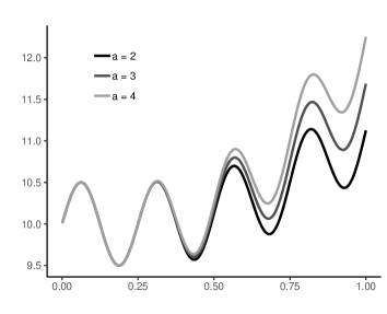
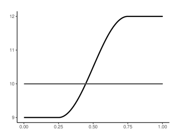
Figure 1. Left: The mean function $\mu_{a}^{\scriptscriptstyle(1)}$ for three choices of $a$. Right: The mean function $\mu^{\scriptscriptstyle(2)}$.

The second model has the mean function

$$\mu^{(2)}(x)=\left\{\begin{array}[]{ll}9&\text{for}~{}x\leq\tfrac{1}{4}\\ -\tfrac{3}{2}\sin(2\pi x)+10.5&\text{for}~{}\tfrac{1}{4}<x\leq\tfrac{3}{4}\\ 12&\text{for}~{}\tfrac{3}{4}<x\end{array}\right.$$ (4.3)

which is displayed in the right part of Figure 1. For models involving this mean function, we considered the testing problem

$$H_{0}:d_{0}=\|\mu^{(2)}-g(\mu)\|_{2,\tau}\leq\Delta\quad\text{ vs.\ }\quad H_{1}:\|\mu^{(2)}-g(\mu)\|_{2,\tau}>\Delta~{}$$ (4.4)

for various choices of the threshold $\Delta>0$, where $g(\mu)\equiv 10$ and $\tau(\cdot)=\lambda_{[0,1]}(\cdot)$ is the Lebesgue measure on the interval $[0,1]$. Such a setting might be encountered in quality control, where deviations from a target value might occur gradually due to wear and tear (and eventual failure) of a component of a complex system. Note that $\|\mu^{(2)}-10\|_{2,\tau}\leq\Delta$ for $\Delta\geq 1.392$, whereas $\|\mu^{(2)}-10\|_{2,\tau}>\Delta$ for $\Delta<1.392$.

$\mu_{a}^{(1)}$		$\tilde{\sigma}^{2}_{0}$			$\tilde{\sigma}^{2}_{1}$			$\tilde{\sigma}^{2}_{2}$			$\tilde{\sigma}^{2}_{3}$
$a$	$d_{0}-\tfrac{1}{2}$	200	500	1000	200	500	1000	200	500	1000	200	500	1000
Panel A: iid errors
0.37	-0.15	0.0	0.0	0.0	0.0	0.0	0.0	0.0	0.0	0.0	0.0	0.2	0.0
0.89	-0.10	0.0	0.1	0.0	0.0	0.2	0.0	0.0	0.0	0.0	0.0	0.2	0.1
1.18	-0.05	0.2	0.9	0.6	0.0	1.0	0.3	0.0	1.4	0.4	0.1	0.9	0.6
1.43	0.00	0.7	3.9	4.5	0.4	2.8	3.4	0.5	5.5	4.6	0.3	2.7	3.4
1.86	0.10	2.7	23.6	43.1	2.1	21.6	33.5	3.0	32.2	47.0	1.0	13.4	26.5
2.26	0.20	7.4	54.6	83.9	8.2	46.3	73.0	9.5	66.5	88.6	3.5	33.4	61.4
2.64	0.30	14.1	76.6	95.8	12.1	68.7	91.8	19.5	88.8	98.0	6.2	51.1	83.1
Panel B: MA errors
0.37	-0.15	0.0	0.0	0.0	0.0	0.0	0.0	0.0	0.0	0.0	0.0	0.0	0.0
0.89	-0.10	0.0	0.0	0.0	0.0	0.0	0.0	0.0	0.0	0.0	0.0	0.0	0.0
1.18	-0.05	0.1	0.4	0.2	0.0	0.8	0.1	0.0	0.2	0.2	0.1	0.2	0.4
1.43	0.00	0.3	4.8	4.9	0.1	4.1	4.2	0.5	7.0	5.3	0.1	4.4	4.1
1.86	0.10	4.3	38.3	58.7	3.7	30.9	53.3	5.5	45.4	69.0	3.0	21.9	39.2
2.26	0.20	12.6	76.8	94.8	11.6	69.3	91.4	16.3	83.8	97.8	9.4	52.5	79.5
2.64	0.30	29.5	93.7	99.9	28.6	87.6	98.8	33.4	97.4	99.7	21.4	75.4	94.0
Panel C: AR errors
0.37	-0.15	0.0	0.0	0.0	0.0	0.0	0.0	0.0	0.0	0.0	0.1	0.0	0.0
0.89	-0.10	0.0	0.3	0.0	0.2	0.1	0.0	0.1	0.3	0.0	0.3	0.6	0.1
1.18	-0.05	0.4	1.3	1.1	0.1	1.5	0.9	0.0	2.3	1.3	0.4	2.4	1.3
1.43	0.00	1.3	8.6	6.5	1.2	7.1	7.5	1.0	7.8	7.0	0.8	5.6	5.8
1.86	0.10	5.3	36.3	52.8	5.4	29.5	47.9	6.8	41.1	57.0	3.9	22.6	35.4
2.26	0.20	16.4	67.8	90.0	14.6	59.9	85.7	18.0	78.2	92.6	10.0	45.0	70.1
2.64	0.30	30.6	86.6	98.9	24.1	80.1	96.1	35.4	92.9	99.4	18.7	65.6	89.5

Table 1. Empirical rejection rates of the test (3.6) for the hypotheses (4.2). The mean function is given by (4.1), where different values for the parameter $a$, different error processes, and sample sizes are considered. The lines in boldface correspond to the boundary of the hypotheses.

We consider four different choices of time-dependent variance $\tilde{\sigma}^{2}(t)=\mathbb{E}[G^{2}(t,\mathcal{F}_{0})]$, that is

$$\tilde{\sigma}_{0}^{2}(t) =1, \tilde{\sigma}_{1}^{2}(t) =\tfrac{1}{2}+t,$$

$$\tilde{\sigma}_{2}^{2}(t) =1-\tfrac{1}{2}\cos(2\pi t), \tilde{\sigma}_{3}^{2}(t) =\tfrac{1}{2}+\mathds{1}(t\geq 1/2)~{},$$

and three classes of error processes $\{{\varepsilon}_{i,n}:1\leq i\leq n\}_{n\in\mathbb{N}}$ in model (1.1), that is

$$(\text{IID})\quad ~{}{\varepsilon}_{i,n}=\tilde{\sigma}_{k}(i/n)\eta_{i}$$

$$(\text{MA)}\quad ~{}{\varepsilon}_{i,n}=\tilde{\sigma}_{k}(i/n)\big{(}\eta_{i}+\tfrac{1}{2}\eta_{i-1}\big{)}/2$$

$$(\text{AR})\quad ~{}{\varepsilon}_{i,n}=\tilde{\sigma}_{k}(i/n)\big{(}\eta_{i}+\tfrac{1}{2}{\varepsilon}_{i-1,n}\big{)}/2,$$

for $k\in\{0,1,2,3\}$, where $(\eta_{i})_{i\in\mathbb{Z}}$ is an i.i.d. sequence of standard normal distributed random variables.

$\mu^{(2)}$		$\tilde{\sigma}^{2}_{0}$			$\tilde{\sigma}^{2}_{1}$			$\tilde{\sigma}^{2}_{2}$			$\tilde{\sigma}^{2}_{3}$
$\Delta$	$\Delta-d_{0}$	200	500	1000	200	500	1000	200	500	1000	200	500	1000
Panel A: iid errors
1.30	-0.09	13.8	41.8	62.8	12.5	36.3	59.4	14.8	47.0	68.4	9.1	23.4	44.3
1.34	-0.05	6.8	20.8	34.3	6.9	19.1	29.8	7.2	22.8	37.6	4.8	11.7	23.3
1.38	-0.01	2.1	8.9	11.2	4.0	8.2	8.3	3.1	8.4	11.2	2.7	4.8	7.9
1.39	0.00	2.0	5.0	5.1	2.2	5.2	5.4	2.4	5.1	5.8	2.4	3.3	4.5
1.41	0.02	1.0	2.6	1.1	1.8	3.0	1.0	1.2	2.6	1.5	1.8	2.0	2.4
1.48	0.09	0.3	0.0	0.0	0.1	0.0	0.0	0.1	0.1	0.0	0.5	0.5	0.0
1.55	0.16	0.1	0.0	0.0	0.0	0.0	0.0	0.0	0.0	0.0	0.1	0.0	0.0
Panel B: MA errors
1.30	-0.09	27.3	58.0	84.6	20.7	54.4	79.7	32.5	67.6	86.3	15.8	40.2	66.1
1.34	-0.05	12.6	30.7	52.3	9.5	26.9	45.9	15.2	37.2	55.7	7.2	18.8	34.5
1.38	-0.01	5.5	11.1	13.7	3.8	8.5	12.6	5.3	11.1	14.8	2.8	7.6	11.7
1.39	0.00	3.0	5.0	7.7	3.4	5.1	6.2	3.6	6.9	7.5	2.2	4.4	5.9
1.41	0.02	1.6	2.0	1.5	1.3	1.2	0.9	1.0	2.0	0.8	1.3	2.3	1.5
1.48	0.09	0.1	0.0	0.0	0.0	0.0	0.0	0.0	0.0	0.0	0.0	0.0	0.0
1.55	0.16	0.0	0.0	0.0	0.0	0.0	0.0	0.0	0.0	0.0	0.0	0.0	0.0
Panel C: AR errors
1.30	-0.09	23.8	52.2	75.0	20.7	43.5	67.8	26.6	58.6	79.2	15.1	36.7	53.6
1.34	-0.05	13.9	28.3	42.8	11.8	23.2	39.3	13.2	32.8	50.1	9.3	22.0	31.1
1.38	-0.01	7.9	10.1	15.3	6.3	8.9	12.8	5.8	12.7	16.8	6.0	10.1	12.5
1.39	0.00	5.7	7.5	9.0	4.5	7.5	8.6	6.3	8.0	9.6	4.2	7.3	9.9
1.41	0.02	3.2	2.6	2.5	2.9	2.4	2.1	2.2	3.3	2.1	3.5	3.7	3.0
1.48	0.09	0.6	0.0	0.0	0.2	0.0	0.0	0.3	0.1	0.0	0.8	0.3	0.1
1.55	0.16	0.1	0.0	0.0	0.0	0.0	0.0	0.0	0.0	0.0	0.1	0.0	0.0

Table 2. Empirical rejection rates of the test (3.6) for the hypotheses (4.4). The mean function is given by (4.3), where different values for the threshold $\Delta$, different error processes, and sample sizes are considered. The lines in boldface correspond to the boundary of the hypotheses.

The empirical rejection rates of the test (3.6) for the hypotheses $H_{0}:d_{0}\leq\Delta$ vs. $H_{0}:d_{0}>\Delta$ are calculated by $N=1000$ simulation runs and displayed in Table 1 and Table 2. The sample size is chosen as $n=200,$ $500$ and $1000$ and the nominal level is $5\%$. Table 1 shows the rejection probabilities for different values of $a$ in the function $\mu_{a}^{(1)}$ defined in (4.1), which yields to different values of $d_{0}$ in the hypotheses (4.2). On the other hand, in Table 2 the function $\mu^{(2)}$ and therefore the value $d_{0}$ is fixed and the threshold $\Delta$ in the hypotheses is varied. The lines marked in boldface indicate the boundary of the null hypothesis, that is, the parameter where $d_{0}=\Delta$. More precisely, note that the null hypothesis in (4.2) holds if and only if $d_{0}\leq 0.5$ and we display exemplary results for the cases $d_{0}=0.35$, $0.4$, $0.45$ and $0.5$ in Table 1, where the last case corresponds to the boundary of the null hypotheses. The remaining cases $d_{0}=0.6$, $0.7$ and $0.8$ represent three scenarios of the alternative in (4.2). Similarly, in Table 2 the function $\mu^{(2)}$ is fixed with $d_{0}=1.39$. Therefore, the null hypothesis in (4.4) holds if and only if the threshold satisfies $\Delta\geq 1.39$. We observe in most cases a good approximation of the nominal level at the boundary of the hypotheses and the test is also able to detect alternatives with reasonable power. These empirical findings corresponds with the theoretical results derived in Section 3.

We conclude this section with a comparison of the new test (3.6) with the test (2.7) which relies on the estimation of the (local) long-run variance. For this purpose we use the long-run variance estimator as proposed in equation (4.7) of Dette and Wu (2019) with bandwidths as suggested in this reference. In Table 3 and 4 we display the rejection probabilities for both tests for some of the models considered in Table 1 and Table 2, where we use the Lebesgue measure on the interval $[0,1]$ for the calculation of the $L^{2}$-distances and the benchmark is given by $g(\mu)=\int_{0}^{1}\mu(x){\mathrm{d}}x$. For the sake of brevity we restrict ourselves to the sample size $n=500$ and the variance function $\tilde{\sigma}_{0}^{2}(t)=1$. We observe that the test (2.7) is conservative at the boundary of the hypotheses. As a consequence the proposed test (3.6) based on self-normalization is usually more powerful.

	errors	i.i.d		MA		AR
$a$	$d_{0}-\Delta$	(3.6)	(2.7)	(3.6)	(2.7)	(3.6)	(2.7)
0.13	-0.15	0.0	0.0	0.0	0.0	0.0	0.0
1.60	-0.10	0.0	0.0	0.0	0.0	0.0	0.0
2.13	-0.05	0.0	0.0	0.1	0.0	0.1	0.0
2.57	0.00	2.2	0.0	1.6	0.0	4.3	0.4
2.97	0.05	14.0	3.0	20.1	0.9	22.6	3.5
3.35	0.10	35.0	24.2	58.1	20.5	46.3	26.8
3.71	0.15	61.9	67.1	84.8	75.7	72.9	71.7

Table 3. Empirical rejection rates of tests (3.6) and (2.7) for the hypotheses (4.2). The mean function is given by (4.1), where different values for the parameter $a$ and different error processes are considered. The variance is $\tilde{\sigma}_{0}^{2}(t)=1$, the sample size is $n=500$ and the line in boldface corresponds to the boundary of the hypotheses.

	errors	i.i.d		MA		AR
$\Delta$	$\Delta-d_{0}$	(3.6)	(2.7)	(3.6)	(2.7)	(3.6)	(2.7)
1.15	-0.15	73.8	83.9	90.3	93.1	81.8	86.2
1.20	-0.10	48.0	45.0	69.3	51.7	58.3	50.4
1.25	-0.05	22.9	10.5	32.1	6.7	31.3	12.4
1.30	0.00	5.5	0.5	4.9	0.1	8.0	0.7
1.35	0.05	0.5	0.0	0.1	0.0	1.4	0.1
1.40	0.10	0.0	0.0	0.0	0.0	0.1	0.0
1.45	0.15	0.0	0.0	0.0	0.0	0.0	0.0

Table 4. Empirical rejection rates of tests (3.6) and (2.7) for the hypotheses (4.4). The mean function is given by (4.3), where different values for the threshold $\Delta$ and different error processes are considered. The variance is $\tilde{\sigma}_{0}^{2}(t)=1$, the sample size is $n=500$ and the line in boldface corresponds to the boundary of the hypotheses.

4.2. Case Study

Time series with possibly smoothly varying mean naturally arise in the field of meteorology. To illustrate the proposed methodology, we consider the mean of daily minimal temperatures (in degrees Celsius) over the month of July for a period of approximately 120 years in eight different places in Australia. At each station we tested for relevant deviations of the temperature from the mean temperature calculated for an historic reference period ranging from the late 19th century to 1925 at that station. As a threshold $\Delta$, we chose $0.25$, $0.5$ and $0.75$ degrees Celsius. Exemplary, the observed temperature curves at the weather station in Cape Otway, Gayndah and Melbourne and the mean over all weather stations are plotted in Figure 2, alongside with their estimated smooth mean curves $\tilde{\mu}$ and the estimated benchmarks $\hat{g}$.

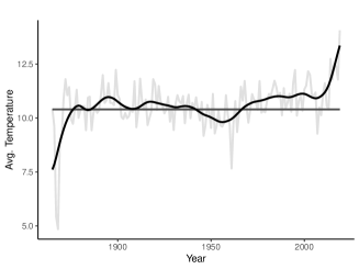
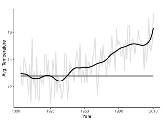
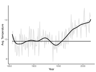
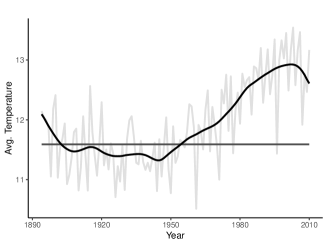
Figure 2. Raw data of the temperature (light grey), estimated benchmark (dark grey) and estimated smooth mean function for different weather stations. Top left: Cape Otway. Top right: Gayndah. Bottom left: Melbourne. Bottom right: Australia (mean).

The results for all stations under consideration can be found in Table 5. For test (3.6), most $p$-values are significant for $\Delta=0.25$ degrees Celsius. Further, two $p$-values for $\Delta=0.5$ are significant. The test (2.7) does not yield a significant $p$-value below $0.05$ at any station. Test (3.6) based on the proposed self-normalization procedure seems to be more powerful than (2.7), which confirms the numerical findings of the simulation study.

Test	(3.6)			(2.7)
$\Delta$	0.25	0.5	0.75	0.25	0.5	0.75
Boulia Airport	4.2	7.8	24.2	22.1	28.5	40.8
Cape Otway Lighthouse	7.3	99.3	100.0	41.6	70.1	96.1
Gayndah Post Office	0.7	1.5	8.4	11.7	18.3	33.3
Gunnedah Pool	0.1	0.5	11.8	13.5	22.2	41.9
Hobart	5.9	53.7	98.6	25.5	51.1	87.9
Melbourne	2.3	59.1	99.7	29.5	51.5	84.1
Robe	48.8	99.6	100.0	49.7	85.8	99.8
Sydney	2.3	98.4	100.0	39.0	62.6	90.6
Australia (mean)	0.4	99.8	100.0	37.4	65.5	94.5

Table 5. $p$-values of tests (3.6) and (2.7) for the respective null hypotheses in percent. Significant $p$-values (below 0.05) are in boldface.

Acknowledgements This work has been supported in part by the Collaborative Research Center “Statistical modeling of nonlinear dynamic processes” (SFB 823, Project A1, C1) of the German Research Foundation (DFG).

Appendix A Proofs of main results

In this section we will provide proofs of the theoretical statements in this paper. We begin with some preliminary results regarding the uniform approximation of the sequential estimators of the regression function, which are of own interest and required for the proofs of the main results in Section 3, which will be given in Section A.3 and A.2.

A.1. Sequential estimators of the regression function

Recall the definition of the sequential Jackknife estimator $\tilde{\mu}_{h_{n}}(\lambda,t)$ in (3.2) and define

$$K^{*}(x)=2\sqrt{2}K(\sqrt{2}x)-K(x)$$ (A.1)

as the corresponding kernel. The following two results provide stochastic expansions for the difference $\tilde{\mu}_{h_{n}}-\mu$ uniformly with respect to $\lambda$ and $t$. Lemma A.1 considers the case where the argument $t$ stays away from the boundary, while a stochastic expansion for the other case is derived in Lemma A.2 below.

Lemma A.1.

Let $h_{n}\to 0$ and $b_{n}\to\infty$ be sequences with $b_{n}=o(nh_{n})$ and define $I_{n}=[h_{n},1-h_{n}]$. If Assumptions 2.1, 2.2 and 2.3 are satisfied, we have

$$\sup_{t\in I_{n},\lambda\in[\zeta,1]}\Big{|}\lambda\big{(}\tilde{\mu}_{h_{n}}(\lambda,t)-\mu(t)\big{)}-\frac{1}{nh_{n}}\sum_{i=1}^{\lfloor\lambda n\rfloor}{\varepsilon}_{T_{i},n}K^{*}_{h_{n}}(T_{i}/n-t)\Big{|}=\mathcal{O}\big{(}h_{n}^{3}+\tfrac{b_{n}}{nh_{n}}\big{)},$$

where $K^{*}_{h_{n}}(\cdot)=K^{*}(\cdot/h_{n})$ and $K^{*}$ is defined in (A.1)

Proof.

Define

$$S_{n,j}(\lambda,t)=\sum_{i=1}^{\lfloor\lambda n\rfloor}\big{(}\tfrac{T_{i}-nt}{nh_{n}}\big{)}^{j}K_{h_{n}}\big{(}\tfrac{T_{i}}{n}-t\big{)}\quad\text{and}\quad R_{n,j}(\lambda,t)=\sum_{i=1}^{\lfloor\lambda n\rfloor}X_{T_{i},n}\big{(}\tfrac{T_{i}-nt}{nh_{n}}\big{)}^{j}K_{h_{n}}\big{(}\tfrac{T_{i}}{n}-t\big{)},$$

for $j\in\{0,1,2\}$. Note that for the calculation of the local linear estimator $\hat{\mu}_{h_{n}}(\lambda,t)$ in (3.1) we have to minimize the function

$$f(b_{0},b_{1})=\sum_{i=1}^{\lfloor\lambda n\rfloor}\big{(}X_{T_{i},n}-b_{0}-b_{1}(T_{i}/n-t)\big{)}^{2}K_{h_{n}}(T_{i}/n-t),$$

which is differentiable with partial derivatives

$$\frac{\partial f}{\partial b_{j}}(b_{0},b_{1})=-2h_{n}^{j}\big{(}R_{n,j}(\lambda,t)-b_{0}S_{n,j}(\lambda,t)-b_{1}h_{n}S_{n,j+1}(\lambda,t)\big{)},$$

for $j\in\{0,1\}$ and Hessian matrix

$$\mathbf{H}_{f}=2\left(\begin{array}[]{cc}S_{n,0}(\lambda,t)&h_{n}S_{n,1}(\lambda,t)\\ h_{n}S_{n,1}(\lambda,t)&h_{n}^{2}S_{n,2}(\lambda,t)\end{array}\right).$$ (A.2)

In the following discussion we will show that

$$\sup_{\lambda\in[\zeta,1]}\bigg{|}\frac{1}{nh_{n}}S_{n,j}(\lambda,t)-\lambda\int_{-1}^{1}x^{j}K(x){\mathrm{d}}x\bigg{|}=\mathcal{O}\big{(}\tfrac{b_{n}}{nh_{n}}\big{)},$$ (A.3)

for $j\in\{0,1,2\}$. If this result is true, the proof follows by arguments similar to those used in the proof of Lemma B.1 of Dette et al. (2019). To be precise, note that

$$S_{n,0}(\lambda,t)S_{n,2}(\lambda,t)-S_{n,1}^{2}(\lambda,t)>0$$

for any $\lambda\in[\zeta,1]$ and almost every $n\in\mathbb{N}$. This means, that the Hessian matrix $\mathbf{H}_{f}$ is positive definite and both partial derivatives vanish if any only if

$$\left(\begin{array}[]{cc}b_{0}\\ b_{1}\end{array}\right)=\left(\begin{array}[]{cc}S_{n,0}(\lambda,t)&h_{n}S_{n,1}(\lambda,t)\\ S_{n,1}(\lambda,t)&h_{n}S_{n,2}(\lambda,t)\end{array}\right)^{-1}\left(\begin{array}[]{cc}R_{n,0}(\lambda,t)\\ R_{n,1}(\lambda,t)\end{array}\right).$$ (A.4)

By (A.3) and a Taylor expansion, it follows that

$$\sup_{t\in I_{n},\lambda\in[\zeta,1]}\Big{|}\lambda\big{(}\hat{\mu}_{h_{n}}(\lambda,t)-\mu(t)\big{)}-\frac{1}{nh_{n}}\sum_{i=1}^{\lfloor\lambda n\rfloor}{\varepsilon}_{T_{i},n}K_{h_{n}}(T_{i}/n-t)-\frac{\lambda}{2}h_{n}^{2}\mu^{\prime\prime}(t)\int_{-1}^{1}x^{2}K(x){\mathrm{d}}x\Big{|}\\ =\mathcal{O}\big{(}h_{n}^{3}+\tfrac{b_{n}}{nh_{n}}\big{)}.$$

The statement of Lemma A.1 now follows from the definition of the Jackknife estimator $\tilde{\mu}_{h_{n}}$ in (3.2).

To finish the proof, we now show the remaining estimate (A.3). For this purpose let $\lambda\in[\zeta,1]$ and define $B(\lambda)=\bigcup_{j=1}^{\ell_{n}}B_{j}(\lambda)$, where the sets $B_{j}(\lambda)$ are defined by

$$B_{j}(\lambda)=\Big{\{}(j-1)b_{n}+1,\dots,(j-1)b_{n}+\lfloor\tfrac{\lambda n-1}{\ell_{n}}\rfloor+\mathds{1}(j-1\leq\lfloor\lambda n\rfloor-1\mod\ell_{n})\Big{\}}.$$

Note that (by Assumption 2.2) the kernel $K$ is Lipschitz continuous with support $[-1,1]$, which implies

$$K\big{(}\tfrac{i-nt}{nh_{n}}\big{)}=\left\{\begin{array}[]{ll}K\big{(}\tfrac{jb_{n}-nt}{nh_{n}}\big{)}+\mathcal{O}\big{(}\tfrac{b_{n}}{nh_{n}}\big{)}&\text{if}~{}\big{|}i-nt\big{|}\leq nh_{n},\\ 0&\text{else,}\end{array}\right.$$

for $i\in B_{j}(\lambda)$, where the error term $\mathcal{O}(\tfrac{b_{n}}{nh_{n}})$ only depends on the function $K$ and, in particular, does not depend on $\lambda$. Thus, if follows that

$$S_{n,k}(\lambda,t) =\sum_{i=1}^{\lfloor\lambda n\rfloor}\big{(}\tfrac{T_{i}-nt}{nh_{n}}\big{)}^{k}K_{h_{n}}\big{(}\tfrac{T_{i}}{n}-t\big{)}=\sum_{i\in B(\lambda)}\big{(}\tfrac{i-nt}{nh_{n}}\big{)}^{j}K_{h_{n}}\big{(}\tfrac{i}{n}-t\big{)}$$

$$=\sum_{j=1}^{\ell_{n}}\sum_{i\in B_{j}(\lambda)}\big{(}\tfrac{i-nt}{nh_{n}}\big{)}^{k}K_{h_{n}}\big{(}\tfrac{i}{n}-t\big{)}$$

$$=\sum_{j=1}^{\ell_{n}}\Big{(}\lfloor\tfrac{\lambda n-1}{\ell_{n}}\rfloor+\mathds{1}\big{(}j-1\leq\lfloor\lambda n\rfloor-1\mod\ell_{n}\big{)}\Big{)}\big{(}\tfrac{jb_{n}-nt}{nh_{n}}\big{)}^{k}K_{h_{n}}\big{(}\tfrac{jb_{n}}{n}-t\big{)}+\mathcal{O}(b_{n}),$$

uniformly in $\lambda$. As the kernel $K$ has support $[-1,1]$ the only non-zero summands in the last expression are those with index $j\in[\tfrac{n(t-h_{n})}{b_{n}},\tfrac{n(t+h_{n})}{b_{n}}]$. Moreover, it holds that

$$\sup_{\lambda\in[\zeta,1]}\bigg{|}\frac{\lambda}{\ell_{n}h_{n}}\sum_{j=-\lfloor\ell_{n}h_{n}\rfloor}^{\lfloor\ell_{n}h_{n}\rfloor}\big{(}\tfrac{jb_{n}}{nh_{n}}\big{)}^{j}K\big{(}\tfrac{jb_{n}}{nh_{n}}\big{)}-\lambda\int_{-1}^{1}x^{j}K(x){\mathrm{d}}x\bigg{|}=\mathcal{O}\big{(}\tfrac{b_{n}}{nh_{n}}\big{)},$$

which implies (A.3). ∎

Lemma A.2.

Let $I_{n}^{c}=[0,1]\setminus I_{n}$, $\kappa_{j,h_{n}}(t)=\int_{-t/h_{n}}^{(1-t)/h_{n}}x^{j}K(x){\mathrm{d}}x$, for $j\in\mathbb{N}_{0}$, and

$$c_{h_{n},i}(t)=\frac{\kappa_{2,h_{n}}(t)-\kappa_{1,h_{n}}(t)\Big{(}\frac{T_{i}-nt}{nh_{n}}\Big{)}}{\kappa_{0,h_{n}}(t)\kappa_{2,h_{n}}(t)-\kappa_{1,h_{n}}^{2}(t)},$$

for $i\in\{1,\dots,n\}$. If the assumptions of Lemma A.1 are satisfied, it holds

$$\sup_{\begin{subarray}{c}t\in I_{n}^{c},\\ \lambda\in[\zeta,1]\end{subarray}}\Big{|}\lambda\big{(}\tilde{\mu}_{h_{n}}(\lambda,t)-\mu(t)\big{)}-\frac{1}{nh_{n}}\sum_{i=1}^{\lfloor\lambda n\rfloor}{\varepsilon}_{T_{i},n}\Big{\{}2c_{\frac{h_{n}}{\sqrt{2}},i}(t)K_{\frac{h_{n}}{\sqrt{2}}}\big{(}\tfrac{T_{i}}{n}-t\big{)}-c_{h_{n},i}(t)K_{h_{n}}\big{(}\tfrac{T_{i}}{n}-t\big{)}\Big{\}}\Big{|}\\ =\mathcal{O}\big{(}h_{n}^{2}+\tfrac{b_{n}}{nh_{n}}\big{)}.$$ (A.5)

Proof.

By similar arguments as given for the approximation in (A.3) it follows that

$$\sup_{t\in I_{n}^{c}}\sup_{\lambda\in[\zeta,1]}\bigg{|}\frac{1}{nh_{n}}S_{n,j}(\lambda,t)-\lambda\kappa_{j,h_{n}}(t)\bigg{|}=\mathcal{O}\big{(}\tfrac{b_{n}}{nh_{n}}\big{)},$$ (A.6)

for $j\in\{0,1,2\}$. Note that $S_{n,0}(\lambda,t)S_{n,2}(\lambda,t)-S_{n,1}^{2}(\lambda,t)>0$ for any $\lambda\in[\zeta,1]$ and almost every $n\in\mathbb{N}$ since, by Assumption 2.2,

$$\int_{\mathcal{A}}K(x){\mathrm{d}}x\int_{\mathcal{A}}x^{2}K(x){\mathrm{d}}x-\bigg{(}\int_{\mathcal{A}}xK(x){\mathrm{d}}x\bigg{)}^{2}=\frac{1}{2}\int_{\mathcal{A}^{2}}(x-y)^{2}K(x)K(y){\mathrm{d}}(x,y),$$

is positive for any set $\mathcal{A}\subset[-1,1]$ with positive Lebesgue measure. Thus, the Hessian matrix $\mathbf{H}_{f}$, as defined in (A.2), is positive definite and the partial derivatives vanish if and only if (A.4) holds true. Therefore, by (A.6) and similar arguments as given in the proof of Lemma B.2 in Dette et al. (2019) we obtain that

$$\sup_{t\in I_{n}^{c},\lambda\in[\zeta,1]}\Big{|}\lambda\big{(}\hat{\mu}_{h_{n}}(\lambda,t)-\mu(t)\big{)}-\frac{1}{nh_{n}}\sum_{i=1}^{\lfloor\lambda n\rfloor}{\varepsilon}_{T_{i},n}c_{h_{n},i}(t)K^{*}_{h_{n}}(T_{i}/n-t)\Big{|}=\mathcal{O}\big{(}h_{n}^{2}+\tfrac{b_{n}}{nh_{n}}\big{)}$$

Finally the statement (A.5) follows from the definition of the Jackknife estimator in (3.2).

∎

A.2. Proof of Theorem 3.4

The following two Lemmas A.3 and A.4 establish the convergence of the finite dimensional distributions and equicontinuity of the process $\{G_{n}(\lambda)\}_{\lambda\in[\zeta,1]}$ in (3.4) (for any $\zeta>0$). The assertion of Theorem 3.4 then follows directly from Theorems 1.5.4 and 1.5.7 of van der Vaart and Wellner (1996).

Lemma A.3.

Let Assumptions 2.1, 2.2, 2.3, 3.1 and 3.2 be satisfied and $\zeta\leq\lambda_{1}\leq\dots\leq\lambda_{p}\leq 1$.Then,

$$\big{(}G_{n}(\lambda_{1}),\dots,G_{n}(\lambda_{p})\big{)}^{\top}\rightsquigarrow\big{(}G(\lambda_{1}),\dots,G(\lambda_{p})\big{)}^{\top}$$

in $\mathbb{R}^{p}$, where the Gaussian process $\{G(\lambda)\}_{\lambda\in[\xi,1]}$ is defined in (3.5)

Proof.

First observe that

$$G_{n}(\lambda)=\lambda\sqrt{n}\big{(}\|\hat{d}_{n}(\lambda,\cdot)-d\|_{2,\tau}^{2}+2\langle d,\hat{d}_{n}(\lambda,\cdot)-d\rangle_{\tau}\big{)},$$

and note that

$$\hat{g}_{n}(\lambda)-g(\mu)=\mathcal{O}_{\mathbb{P}}(n^{-1/2})$$ (A.7)

by Assumptions 2.3 and 3.1. Recall the definition of the interval $I_{n}=[h_{n},1-h_{n}]$ and denote $\langle f,g\rangle_{I_{n}}=\int_{I_{n}}f(x)g(x)\tau({\mathrm{d}}x)$ and $\|f\|_{2,I_{n}}=\langle f,f\rangle_{I_{n}}^{1/2}$, for any $f,g\in L^{2}([0,1],\tau)$. In the following let

$$\tilde{G}_{n}(\lambda)=\lambda\sqrt{n}\big{(}\|\hat{d}_{n}(\lambda,\cdot)-d\|_{2,I_{n}}^{2}+2\langle d,\hat{d}_{n}(\lambda,\cdot)-d\rangle_{I_{n}}\big{)}~{},$$ (A.8)

then the assertion follows from the statements

$$(\tilde{G}_{n}(\lambda_{1}),\ldots,\tilde{G}_{n}(\lambda_{p}))^{\top} \rightsquigarrow(G(\lambda_{1}),\ldots,G(\lambda_{p}))^{\top}$$ (A.9)

$$\sup_{\lambda\in[\zeta,1]}|\tilde{G}_{n}(\lambda)-G_{n}(\lambda)| =o_{\mathbb{P}}(1)$$ (A.10)

For a proof of (A.9) note that by the Cramér-Wold device, it is sufficient to prove

$$\sum_{i=1}^{p}a_{i}\tilde{G}_{n}(\lambda_{i})\rightsquigarrow\sum_{i=1}^{p}a_{i}G(\lambda_{i})$$

for all $a_{1},\dots,a_{p}\in\mathbb{R}$. Define $S_{k}=\sum_{i=1}^{k}{\varepsilon}_{i,n}$ and $\tilde{S}_{k}=\sum_{i=1}^{k}\tilde{\varepsilon}_{i,n}$ with

$$\tilde{{\varepsilon}}_{i,n}=\mathbb{E}[{\varepsilon}_{i,n}|\eta_{i},\dots,\eta_{i-m_{n}}]$$ (A.11)

for $m_{n}\in\mathbb{N}$ and $k=1,\dots,n$. By Assumption 2.3 (1), Assumption 3.2 and equation (3.2) of Wu and Zhou (2011) we have

$$\big{\|}\max_{1\leq k\leq n}|\tilde{S}_{k}-S_{k}|\big{\|}_{8,\Omega}=\mathcal{O}(n^{1/2}m_{n}^{-c}),$$ (A.12)

where $m_{n}=n^{\gamma}$ with $\gamma<{\min}\{\beta/4,\alpha/2\}$ and the constant $c$ is given by $c=\frac{5}{6\gamma}$. In particular, the sequences $\frac{m_{n}^{4}}{nh_{n}^{4}},\frac{m_{n}^{2}}{b_{n}}$ and $\frac{b_{n}n^{1/2}}{m_{n}^{c}}$ are all of order $o(1)$ as $n$ tends to infinity. From Lemma A.1 it follows that

$$\sup_{t\in[h_{n},1-h_{n}],\lambda\in[\zeta,1]}\Big{|}\lambda\big{(}\tilde{\mu}_{h_{n}}(\lambda,t)-\mu(t)\big{)}-\frac{1}{nh_{n}}\sum_{i=1}^{\lfloor\lambda n\rfloor}{\varepsilon}_{T_{i},n}K^{*}_{h_{n}}(T_{i}/n-t)\Big{|}=\mathcal{O}\big{(}h_{n}^{3}+\tfrac{b_{n}}{nh_{n}}\big{)}.$$ (A.13)

Observe that by Assumption 3.1, (A.7), (A.12) and (A.13)

$$\lambda\sqrt{n}\|\hat{d}_{n}(\lambda,\cdot)-d\|_{2,I_{n}}^{2}=\frac{\sqrt{n}}{\lambda}\bigg{\|}\bigg{(}\frac{1}{n}\sum_{j=1}^{\lfloor\lambda n\rfloor}{{\varepsilon}}_{T_{j},n}\frac{1}{h_{n}}K_{h_{n}}^{*}(T_{j}/n-\cdot)\bigg{)}+\lambda(\hat{g}_{n}(\lambda)-g(\mu))\bigg{\|}_{2,I_{n}}^{2}+o_{\mathbb{P}}(1)$$ (A.14)

$$\leq 2\frac{\sqrt{n}}{\lambda}\bigg{\|}\frac{1}{n}\sum_{j=1}^{\lfloor\lambda n\rfloor}{{\varepsilon}}_{T_{j},n}\frac{1}{h_{n}}K_{h_{n}}^{*}(T_{j}/n-\cdot)\bigg{\|}^{2}_{2,I_{n}}+2\sqrt{n}\lambda(\hat{g}_{n}(\lambda)-g(\mu))^{2}+o_{\mathbb{P}}(1)$$

$$= 2\frac{\sqrt{n}}{\lambda}\bigg{\|}\frac{1}{n}\sum_{j=1}^{\lfloor\lambda n\rfloor}{\tilde{\varepsilon}}_{T_{j},n}\frac{1}{h_{n}}K_{h_{n}}^{*}(T_{j}/n-\cdot)\bigg{\|}^{2}_{2,I_{n}}+o_{\mathbb{P}}(1)$$

uniformly with respect to $\lambda\in[\zeta,1]$, where the random variables $\tilde{\varepsilon}_{T_{j},n}$ are defined in (A.11) and $m_{n}$-dependent in the sense that $\tilde{\varepsilon}_{T_{j_{1}},n}$ and $\tilde{\varepsilon}_{T_{j_{2}},n}$ are independent if $|T_{j_{1}}-T_{j_{2}}|>m_{n}$. For the estimation of the first term, let $K_{i,j}$ denote the integral $\int_{I_{n}}K_{h_{n}}^{*}(T_{i}/n-x)K_{h_{n}}^{*}(T_{j}/n-x)\tau({\mathrm{d}}x)$. By the Cauchy-Schwarz inequality and absolute continuity of $\tau$, $K_{i,j}$ can be bounded from above by $Ch_{n}$. Tith implies

$$\begin{split}&\mathbb{E}\bigg{[}\sup_{\lambda\in[\zeta,1]}n^{2}\bigg{\|}\frac{1}{nh_{n}}\sum_{j=1}^{\lfloor\lambda n\rfloor}\tilde{\varepsilon}_{T_{j},n}K_{h_{n}}^{*}(T_{j}/n-\cdot)\bigg{\|}_{2,I_{n}}^{8}\bigg{]}\\ &\leq\sum_{k=1}^{n}\frac{n^{2}}{n^{8}h_{n}^{8}}\mathbb{E}\bigg{[}\bigg{\|}\sum_{j=1}^{k}\tilde{{\varepsilon}}_{T_{j},n}K_{h_{n}}^{*}(T_{j}/n-\cdot)\bigg{\|}_{2,I_{n}}^{8}\bigg{]}\\ &=\sum_{k=1}^{n}\frac{1}{n^{6}h_{n}^{8}}\sum_{j_{1},\dots,j_{8}=1}^{k}\mathbb{E}\bigg{[}\prod_{r=1}^{8}\tilde{{\varepsilon}}_{T_{j_{r}},n}\bigg{]}K_{j_{1},j_{2}}K_{j_{3},j_{4}}K_{j_{5},j_{6}}K_{j_{7},j_{8}}=\mathcal{O}(\tfrac{m_{n}^{4}}{nh_{n}^{4}}),\end{split}$$ (A.15)

where the last estimate follows observing $\max_{1\leq i\leq n}\mathbb{E}{\varepsilon}_{i,n}^{8}<\infty$ by Assumption 2.3 (4) and the fact that only $\mathcal{O}(n^{4}m_{n}^{4})$ summands of the inner sum are non-zero due to the $m_{n}$-dependency of the random variables $\tilde{\varepsilon}_{j,n}$. Thus, by (A.14),

$$\lambda\sqrt{n}\|\hat{d}_{n}(\lambda,\cdot)-d\|_{2,I_{n}}^{2}=o_{\mathbb{P}}(1)$$ (A.16)

uniformly with respect to $\lambda\in[\zeta,1]$. If

$$d_{0}=\int_{0}^{1}d^{2}(x)dx=0,$$

it follows that $G_{n}(\lambda)=o_{\mathbb{P}}(1)$ and therefore we assume $d_{0}>0$ in the following discussion. In this case we have from (A.8) and (A.13) that

$$\sum_{i=1}^{p}a_{i}\tilde{G}_{n}(\lambda_{i})=2\sum_{i=1}^{p}a_{i}\lambda_{i}\sqrt{n}\langle d,\hat{d}_{n}(\lambda,\cdot)-d\rangle_{I_{n}}+o_{\mathbb{P}}(1)=Z_{n}+o_{\mathbb{P}}(1),$$ (A.17)

where

$$Z_{n}=\frac{2}{\sqrt{n}}\sum_{i=1}^{p}a_{i}\sum_{j=1}^{\lfloor\lambda_{i}n\rfloor}\tilde{{\varepsilon}}_{T_{j},n}\langle d,h_{n}^{-1}K_{h_{n}}^{*}(T_{j}/n-\cdot)+\omega_{n}(T_{j}/n)\rangle_{I_{n}}.$$

By Lipschitz continuity of $d$ and $\textnormal{supp}(K)=[-1,1]$ it follows that

$$\int_{I_{n}}d(x)K_{h_{n}}^{*}(T_{j}/n-x)\tau({\mathrm{d}}x)\\ =\Big{(}d\big{(}\tfrac{T_{j}}{n}\big{)}+\mathcal{O}(h_{n})\Big{)}\int_{I_{n}}K_{h_{n}}^{*}(T_{j}/n-x)\tau({\mathrm{d}}x).$$

We obtain for any point of continuity $y$ of the piecewise continuous density $f_{\tau}$ of the measure $\tau$ that

$$\frac{1}{h_{n}}\int_{I_{n}}K_{h_{n}}^{*}(y-x)\tau({\mathrm{d}}x) =\frac{1}{h_{n}}\int_{h_{n}}^{1-h_{n}}K_{h_{n}}^{*}(y-x)f_{\tau}(x){\mathrm{d}}x$$

$$=\int_{1-y/h_{n}}^{1/h_{n}-1-y/h_{n}}K^{*}(x)f_{\tau}(xh_{n}+y){\mathrm{d}}x$$

$$=\left\{\begin{array}[]{ll}f_{\tau}(y)+o(1),&\text{if}~{}y\in[2h_{n},1-2h_{n}],\\ \mathcal{O}(1),&\text{else}.\end{array}\right.$$

Therefore, for $T_{j}\in\{2nh_{n},\dots,n-2nh_{n}\}$, it holds

$$\frac{1}{h_{n}}\int_{I_{n}}d(x)K_{h_{n}}^{*}(T_{j}/n-x)\tau({\mathrm{d}}x)=f_{\tau}(T_{j}/n)d(T_{j}/n)+o(1),$$ (A.18)

which leads to

$$Z_{n} =\sum_{j=1}^{n}Y_{j}+o_{\mathbb{P}}(1)$$ (A.19)

where the random variables $Y_{1},\dots,Y_{n}$ are defined by

$$Y_{j}=\frac{2}{\sqrt{n}}\bigg{(}\sum_{i=1}^{p}a_{i}\mathds{1}\big{(}j\leq\lfloor\lambda_{i}n\rfloor\big{)}\bigg{)}\tilde{{\varepsilon}}_{T_{j},n}d_{\omega_{n}}(T_{j}/n)\qquad(j=1,\dots,n)$$

and

$$d_{\omega_{n}}(T_{j}/n)=f_{\tau}(T_{j}/n)d(T_{j}/n)+\omega_{n}(T_{j}/n)\int_{0}^{1}d(x)\tau({\mathrm{d}}x).$$

Observe that $Y_{1},\dots,Y_{n}$ centred and $m_{n}$-dependent random variables in the sense that $Y_{j_{1}}$ and $Y_{j_{2}}$ are independent if $|T_{j_{1}}-T_{j_{2}}|>m_{n}$. Define the big blocks $B_{j}=\{k\in\mathbb{N}:(j-1)b_{n}+1\leq k\leq jb_{n}-m_{n}\}$ and the small blocks $S_{j}=\{k\in\mathbb{N}:jb_{n}-m_{n}+1\leq k\leq jb_{n}\}$, for $j=1\dots,\ell_{n}$, and the remainder $R=\{k\in\mathbb{N}:\ell_{n}b_{n}+1\leq k\leq n\}$. In the following, we will show that the small blocks and the remainder are negligible and the asymptotic behaviour of $Z_{n}$ is determined by the big blocks. First observe that $\tilde{{\varepsilon}}_{T_{k_{1}},n}\in S_{j_{1}}$ and $\tilde{{\varepsilon}}_{T_{k_{2}},n}\in S_{j_{2}}$ are independent for $j_{1}\neq j_{2}$. Thus,

$$\begin{split}&\mathbb{E}\bigg{[}\bigg{(}\sum_{j=1}^{\ell_{n}}\sum_{k:T_{k}\in S_{j}}Y_{k}\bigg{)}^{2}\bigg{]}\\ &=\sum_{j=1}^{\ell_{n}}\sum_{k_{1}:T_{k_{1}}\in S_{j}}\sum_{k_{2}:T_{k_{2}}\in S_{j}}\mathbb{E}[Y_{k_{1}}Y_{k_{2}}]\\ &=\frac{4}{n}\sum_{j=1}^{\ell_{n}}\sum_{i_{1},i_{2}=1}^{p}a_{i_{1}}a_{i_{2}}\sum_{k_{1}=1}^{\lfloor\lambda_{i_{1}}n\rfloor}\sum_{k_{2}=1}^{\lfloor\lambda_{i_{2}}n\rfloor}\mathds{1}(T_{k_{1}},T_{k_{2}}\in S_{j})\mathbb{E}[\tilde{{\varepsilon}}_{T_{k_{1}},n}\tilde{{\varepsilon}}_{T_{k_{2}},n}]d_{\omega_{n}}(T_{k_{1}}/n)d_{\omega_{n}}(T_{k_{2}}/n).\end{split}$$ (A.20)

Further, $T_{k}\in S_{j}$ for some $k\leq\lfloor\lambda n\rfloor$, if and only if $k=r\ell_{n}+j$ for some $r\geq b_{n}-m_{n}$ and $r\leq\lfloor\tfrac{\lambda n-j}{\ell_{n}}\rfloor$ and we obtain

$$\begin{split}&\mathbb{E}\bigg{[}\bigg{(}\sum_{j=1}^{\ell_{n}}\sum_{k:T_{k}\in S_{j}}Y_{k}\bigg{)}^{2}\bigg{]}\\ &=\sum_{i_{1},i_{2}=1}^{p}a_{i_{1}}a_{i_{2}}\frac{4}{n}\sum_{j=1}^{\ell_{n}}\sum_{r_{1}=b_{n}-m_{n}}^{\lfloor\tfrac{\lambda_{i_{1}}n-j}{\ell_{n}}\rfloor}\sum_{r_{2}=b_{n}-m_{n}}^{\lfloor\tfrac{\lambda_{i_{2}}n-j}{\ell_{n}}\rfloor}d_{\omega_{n}}\big{(}\tfrac{(j-1)b_{n}+r_{1}+1}{n}\big{)}d_{\omega_{n}}\big{(}\tfrac{(j-1)b_{n}+r_{2}+1}{n}\big{)}\\ &\hskip 28.45274pt\times\mathbb{E}[\tilde{{\varepsilon}}_{(j-1)b_{n}+r_{1}+1,n}\tilde{{\varepsilon}}_{(j-1)b_{n}+r_{2}+1,n}].\end{split}$$

For $\lambda<1$, it holds that $\lambda\tfrac{n}{b_{n}\ell_{n}}\to\lambda$ and $1-\tfrac{m_{n}}{b_{n}}\to 1$, so for almost every $n\in\mathbb{N}$, $b_{n}-m_{n}\geq\lfloor\tfrac{\lambda n-j}{\ell_{n}}\rfloor$. Thus, if $\lambda_{i_{1}}<1$ or $\lambda_{i_{2}}<1$, the sums indexed by $r_{1}$ and $r_{2}$ on the right-hand side of the previous display are empty sums for almost every $n\in\mathbb{N}$. For $\lambda=1$, there are $m_{n}$ summands in both sums, thus, the right-hand side of the previous display is of order $\mathcal{O}(m_{n}^{2}/b_{n})$ which vanishes by assumption. Thus the small blocks are asymptotically negligible, and analogously,

$$\mathbb{E}\bigg{[}\bigg{(}\sum_{k\in\bar{R}}Y_{k}\bigg{)}^{2}\bigg{]}=\mathcal{O}\Big{(}\frac{b_{n}^{2}}{n}\Big{)}.$$

The sums over the big blocks are independent, and we have analogously to (A.20),

$$\sum_{j=1}^{\ell_{n}}\mathbb{E}\bigg{[}\bigg{(}\sum_{k:T_{k}\in B_{j}}Y_{k}\bigg{)}^{2}\bigg{]}=\sum_{i_{1},i_{2}=1}^{p}a_{i_{1}}a_{i_{2}}\frac{4}{n}\sum_{j=1}^{\ell_{n}}\sum_{r_{1}\in\bar{B}_{i_{1},j}}\sum_{r_{2}\in\bar{B}_{i_{2},j}}d_{\omega_{n}}\big{(}\tfrac{r_{1}}{n}\big{)}d_{\omega_{n}}\big{(}\tfrac{r_{2}}{n}\big{)}\mathbb{E}[\tilde{{\varepsilon}}_{r_{1},n}\tilde{{\varepsilon}}_{r_{2},n}]$$

where

$$\bar{B}_{i,j}=\{(j-1)b_{n}+1,\dots,(j-1)b_{n}+1+\lfloor\tfrac{\lambda_{i}n-j}{\ell_{n}}\rfloor\wedge(b_{n}-m_{n}-1)\},$$

for $\lambda_{i}\in[\zeta,1]$. Note that, for almost every $n\in\mathbb{N}$, $\bar{B}_{i,j}=\{(j-1)b_{n}+1,\dots,(j-1)b_{n}+1+\lfloor\tfrac{\lambda_{i}n-j}{\ell_{n}}\rfloor\}$, if $\lambda<1$ and $\bar{B}_{i,j}=\{(j-1)b_{n}+1,\dots,jb_{n}-m_{n}\}$, if $\lambda=1$. By Lipschitz continuity of $d$ and Assumption 3.1,

$$\sum_{j=1}^{\ell_{n}}\mathbb{E}\bigg{[}\bigg{(}\sum_{k:T_{k}\in B_{j}}Y_{k}\bigg{)}^{2}\bigg{]}=\sum_{i_{1},i_{2}=1}^{p}a_{i_{1}}a_{i_{2}}\frac{4}{n}\sum_{j=1}^{\ell_{n}}d_{\omega_{n}}^{2}\big{(}\tfrac{jb_{n}}{n}\big{)}\sum_{r_{1}\in\bar{B}_{i_{1},j}}\sum_{r_{2}\in\bar{B}_{i_{2},j}}\mathbb{E}[\tilde{{\varepsilon}}_{r_{1},n}\tilde{{\varepsilon}}_{r_{2},n}]+\mathcal{O}\big{(}\tfrac{b_{n}^{2}}{nh_{n}}\big{)}.\\$$ (A.21)

Now, by (A.12),

$$\max_{1\leq r_{1},r_{2}\leq n}\big{|}\mathbb{E}[\tilde{{\varepsilon}}_{r_{1},n}\tilde{{\varepsilon}}_{r_{2},n}]-\mathbb{E}[{\varepsilon}_{r_{1},n}{\varepsilon}_{r_{2},n}]\big{|}=\mathcal{O}(n^{1/2}m_{n}^{-c}).$$ (A.22)

Applying Assumption 2.3 (2), yields

$$\mathbb{E}[{\varepsilon}_{r_{1},n}{\varepsilon}_{r_{2},n}]=\mathbb{E}\big{[}G\big{(}\tfrac{jb_{n}}{n},\mathcal{F}_{r_{1}}\big{)}G\big{(}\tfrac{jb_{n}}{n},\mathcal{F}_{r_{2}}\big{)}\big{]}+\mathcal{O}(b_{n}/n),$$

for any $r_{1}\in\bar{B}_{i_{1},j},r_{2}\in\bar{B}_{i_{2},j}$. By the same arguments as in the proof of Theorem 1 in Wu and Pourahmadi (2009) and Assumption 2.3 (1), it follows that

$$\mathbb{E}\big{[}G\big{(}\tfrac{i}{n},\mathcal{F}_{r_{1}}\big{)}G\big{(}\tfrac{i}{n},\mathcal{F}_{r_{2}}\big{)}\big{]}=\mathcal{O}(\gamma^{|r_{2}-r_{1}|}),$$

for any $1\leq i\leq n$, in particular $i=jb_{n}$. Let $b:=|\bar{B}_{i_{1},j}\cap\bar{B}_{i_{2},j}|$, then,

$$\begin{split}\sum_{r_{1}\in\bar{B}_{i_{1},j}}\sum_{r_{2}\in\bar{B}_{i_{2},j}}\mathbb{E}[{\varepsilon}_{r_{1},n}{\varepsilon}_{r_{2},n}]&=b\sum_{k=-b}^{b}\big{(}1-\tfrac{|k|}{b}\big{)}\mathbb{E}\big{[}G\big{(}\tfrac{jb_{n}}{n},\mathcal{F}_{0}\big{)}G\big{(}\tfrac{jb_{n}}{n},\mathcal{F}_{k}\big{)}\big{]}+\mathcal{O}(b_{n}^{3}/n+b_{n}\gamma^{b_{n}}+1)\\ &=(\lambda_{i_{1}}\wedge\lambda_{i_{2}})b_{n}\sigma^{2}\bigg{(}\frac{jb_{n}}{n}\bigg{)}+\mathcal{O}(b_{n}^{3}/n+b_{n}\gamma^{b_{n}}+1).\end{split}$$ (A.23)

Thus, by (A.22),

$$\sum_{r_{1}\in\bar{B}_{i_{1},j}}\sum_{r_{2}\in\bar{B}_{i_{2},j}}\mathbb{E}[\tilde{\varepsilon}_{r_{1},n}\tilde{\varepsilon}_{r_{2},n}]=\big{(}\lambda_{i_{1}}\wedge\lambda_{i_{2}}\big{)}b_{n}\sigma^{2}\bigg{(}\frac{jb_{n}}{n}\bigg{)}+\mathcal{O}\bigg{(}\frac{b_{n}^{3}}{n}+b_{n}\gamma^{b_{n}}+1+\frac{b_{n}^{2}n^{1/2}}{m_{n}^{c}}\bigg{)}.$$

Plugging this into (A.21) and observing $\ell_{n}=\lfloor n/b_{n}\rfloor$ leads to

$$\sum_{j=1}^{\ell_{n}}\mathbb{E}\bigg{[}\bigg{(}\sum_{k:T_{k}\in B_{j}}Y_{k}\bigg{)}^{2}\bigg{]} =\sum_{i_{1},i_{2}=1}^{p}4a_{i_{1}}a_{i_{2}}(\lambda_{i_{1}}\wedge\lambda_{i_{2}})\|d_{\omega}\sigma\|_{2}^{2}+o(1)$$ (A.24)

$$=\textnormal{Var}\bigg{(}\sum_{i=1}^{p}a_{i}G(\lambda_{i})\bigg{)}+o(1).$$

Finally, observe that by Jensen’s inequality and Assumption 2.3 (4), for some constant $C>0$,

$$\sum_{j=1}^{\ell_{n}}\mathbb{E}\bigg{[}\bigg{(}\sum_{k:T_{k}\in B_{j}}Y_{k}\bigg{)}^{4}\bigg{]}\leq\sum_{j=1}^{\ell_{n}}b_{n}^{3}\mathbb{E}\bigg{[}\sum_{k:T_{k}\in B_{j}}Y_{k}^{4}\bigg{]}\leq C\frac{b_{n}^{3}}{n}\max_{k=1}^{n}\mathbb{E}\,\tilde{{\varepsilon}}_{T_{k},n}^{4}=\mathcal{O}(b_{n}^{3}/n).$$

By Lyapunov’s central limit theorem, it follows that

$$Z_{n}\rightsquigarrow\mathcal{N}\bigg{(}0,\textnormal{Var}\bigg{(}\sum_{i=1}^{p}a_{i}G(\lambda_{i})\bigg{)}\bigg{)}\stackrel{{\scriptstyle\mathcal{D}}}{{=}}\sum_{i=1}^{p}a_{i}G(\lambda_{i})$$

and the statement (A.9) is a consequence of (A.17), (A.19) and the Cramér-Wold device.
For the proof of the remaining statement (A.10) we note that this assertion is a consequence of the estimate

$$\sup_{\lambda\in[\zeta,1]}\int_{I_{n}^{c}}\lambda\sqrt{n}\big{(}\tilde{\mu}_{h_{n}}(\lambda,t)-\mu(t)\big{)}^{j}{\mathrm{d}}t=o_{\mathbb{P}}(1)\qquad j\in\{1,2\}.$$ (A.25)

To prove this statement, we note that by Lemma A.2

$$\sup_{\lambda\in[\zeta,1]}\int_{I_{n}^{c}}\lambda\sqrt{n}\big{(}\tilde{\mu}_{h_{n}}(\lambda,t)-\mu(t)\big{)}^{j}{\mathrm{d}}t=\\ \sup_{\lambda\in[\zeta,1]}\int_{I_{n}^{c}}\frac{1}{\lambda^{j-1}}\sqrt{n}\bigg{(}\frac{1}{nh_{n}}\sum_{i=1}^{\lfloor\lambda n\rfloor}{\varepsilon}_{T_{i},n}\Big{(}2c_{\frac{h_{n}}{\sqrt{2}},i}(t)K_{\frac{h_{n}}{\sqrt{2}}}\big{(}\tfrac{T_{i}}{n}-t\big{)}-c_{h_{n},i}(t)K_{h_{n}}\big{(}\tfrac{T_{i}}{n}-t\big{)}\Big{)}\bigg{)}^{j}{\mathrm{d}}t+o(1),$$

for $j\in\{1,2\}$. The case $j=2$ follows by similar arguments as given in (A.15). For the case $j=1$ recall from the previous discussion that the random variables ${\varepsilon}_{i,n}$ can be approximated by $m_{n}$-dependent random variables $\tilde{{\varepsilon}}_{i,n}$. Thus,

$$\begin{split}&\sup_{\lambda\in[\zeta,1]}\int_{I_{n}^{c}}\lambda\sqrt{n}\big{(}\tilde{\mu}_{h_{n}}(\lambda,t)-\mu(t)\big{)}{\mathrm{d}}t\\ &=\sup_{\lambda\in[\zeta,1]}\int_{I_{n}^{c}}\frac{1}{\sqrt{n}h_{n}}\sum_{i=1}^{\lfloor\lambda n\rfloor}\tilde{\varepsilon}_{T_{i},n}\Big{(}2c_{\frac{h_{n}}{\sqrt{2}},i}(t)K_{\frac{h_{n}}{\sqrt{2}}}\big{(}\tfrac{T_{i}}{n}-t\big{)}-c_{h_{n},i}(t)K_{h_{n}}\big{(}\tfrac{T_{i}}{n}-t\big{)}\Big{)}{\mathrm{d}}t+o_{\mathbb{P}}(1)\\ &=\sup_{\lambda\in[\zeta,1]}\frac{1}{\sqrt{n}}\sum_{i=1}^{\lfloor\lambda n\rfloor}\tilde{\varepsilon}_{T_{i},n}\int_{I_{n}^{c}}\frac{1}{h_{n}}\Big{(}2c_{\frac{h_{n}}{\sqrt{2}},i}(t)K_{\frac{h_{n}}{\sqrt{2}}}\big{(}\tfrac{T_{i}}{n}-t\big{)}-c_{h_{n},i}(t)K_{h_{n}}\big{(}\tfrac{T_{i}}{n}-t\big{)}\Big{)}{\mathrm{d}}t+o_{\mathbb{P}}(1)\\ &=\sup_{\lambda\in[\zeta,1]}\frac{1}{\sqrt{n}}\sum_{j\in B}\sum_{i=1}^{\lfloor\lambda b_{n}\rfloor}\tilde{\varepsilon}_{(j-1)b_{n}+i,n}\\ &\hskip 28.45274pt\times\int_{I_{n}^{c}}\frac{1}{h_{n}}\Big{(}2c_{\frac{h_{n}}{\sqrt{2}},i}(t)K_{\frac{h_{n}}{\sqrt{2}}}\big{(}\tfrac{(j-1)b_{n}+i}{n}-t\big{)}-c_{h_{n},i}(t)K_{h_{n}}\big{(}\tfrac{(j-1)b_{n}+i}{n}-t\big{)}\Big{)}{\mathrm{d}}t+o_{\mathbb{P}}(1),\end{split}$$ (A.26)

where $B$ denotes the set $\{1,\dots,\lfloor 2\ell_{n}h_{n}\rfloor\}\cup\{\lfloor\ell_{n}(1-2h_{n})\rfloor,\dots,\ell_{n}\}$. Note that the integral on the right-hand side of (A.26) is bounded and by similar arguments as used in the proof of (A.15), the right-hand side of (A.26) is of order $\mathcal{O}(b_{n}h_{n}^{4}m_{n}^{4})$, which converges to $0$ by the definition of $m_{n}$ and Assumption 3.2.

Therefore (A.25) follows and the proof of Lemma A.3 is completed. ∎

Lemma A.4.

Let Assumptions 2.1, 2.2, 2.3, 3.1 and 3.2 be satisfied. Then,

$$\lim\limits_{\rho\searrow 0}\lim\limits_{n\to\infty}\mathbb{P}(\sup_{|\lambda_{1}-\lambda_{2}|\leq\rho}|G_{n}(\lambda_{1})-G_{n}(\lambda_{2})|>{\varepsilon})=0,$$

for any ${\varepsilon}>0$.

Proof.

By (A.10), it follows that

$$G_{n}(\lambda_{1})-G_{n}(\lambda_{2}) =\tilde{G}_{n}(\lambda_{1})-\tilde{G}_{n}(\lambda_{2})+o_{\mathbb{P}}(1).$$

uniformly with respect to $\lambda\in[\zeta,1]$, where $\tilde{G}_{n}(\lambda)$ is defined in (A.8). Therefore the assertion of the Lemma follows from

$$\lim\limits_{\rho\searrow 0}\lim\limits_{n\to\infty}\mathbb{P}(\sup_{|\lambda_{1}-\lambda_{2}|\leq\rho}|\tilde{G}_{n}(\lambda_{1})-\tilde{G}_{n}(\lambda_{2})|>{\varepsilon})=0,$$ (A.27)

To prove this statement note that we obtain from (A.16)

$$\tilde{G}_{n}(\lambda_{1})-\tilde{G}_{n}(\lambda_{2})=2\sqrt{n}\langle\lambda_{1}\big{(}\hat{d}_{n}(\lambda_{1},\cdot)-d\big{)}-\lambda_{2}\big{(}\hat{d}_{n}(\lambda_{2},\cdot)-d\big{)},d\rangle_{I_{n}}+o_{\mathbb{P}}(1)$$

uniformly with respect to $\lambda_{1},\lambda_{2}\in[\zeta,1]$. By Lemma A.1, Assumption 3.1 and (A.18) we have the expansion

$$\tilde{G}_{n}(\lambda_{1})-\tilde{G}_{n}(\lambda_{2}) =\frac{2}{\sqrt{n}}\sum_{i=\lfloor(\lambda_{1}\wedge\lambda_{2})n\rfloor+1}^{\lfloor(\lambda_{1}\vee\lambda_{2})n\rfloor}{\varepsilon}_{T_{i},n}\bigg{\langle}\frac{1}{h_{n}}K_{h_{n}}^{*}\bigg{(}\frac{T_{i}}{n}-\cdot\bigg{)}+\omega_{n}\bigg{(}\frac{T_{i}}{n}\bigg{)},d\bigg{\rangle}_{I_{n}}+o_{\mathbb{P}}(1)$$

$$=\frac{2}{\sqrt{n}}\sum_{i=\lfloor(\lambda_{1}\wedge\lambda_{2})n\rfloor+1}^{\lfloor(\lambda_{1}\vee\lambda_{2})n\rfloor}{\varepsilon}_{T_{i},n}d_{\omega_{n}}(T_{i}/n)+o_{\mathbb{P}}(1),$$

uniformly in $\lambda_{1},\lambda_{2}\in[\zeta,1]$, where $d_{\omega_{n}}$ is defined in the proof of Lemma A.3. Further, recalling the definition of $\tilde{{\varepsilon}}_{i,n}$ in (A.11), it follows by (A.12), that

$$\tilde{G}_{n}(\lambda_{1})-\tilde{G}_{n}(\lambda_{2})=\frac{2}{\sqrt{n}}\sum_{i=\lfloor(\lambda_{1}\wedge\lambda_{2})n\rfloor+1}^{\lfloor(\lambda_{1}\vee\lambda_{2})n\rfloor}\tilde{\varepsilon}_{T_{i},n}d_{\omega_{n}}(T_{i}/n)+o_{\mathbb{P}}(1)$$

uniformly in $\lambda_{1},\lambda_{2}\in[\zeta,1]$. In particular, we obtain

$$\mathbb{P}\Big{(}\sup_{|\lambda_{1}-\lambda_{2}|\leq\rho}|\tilde{G}_{n}(\lambda_{1})-\tilde{G}_{n}(\lambda_{2})|>{\varepsilon}\Big{)}\\ =\mathbb{P}\bigg{(}\sup_{|\lambda_{1}-\lambda_{2}|\leq\rho}\bigg{|}\frac{2}{\sqrt{n}}\sum_{i=\lfloor(\lambda_{1}\wedge\lambda_{2})n\rfloor+1}^{\lfloor(\lambda_{1}\vee\lambda_{2})n\rfloor}\tilde{\varepsilon}_{T_{i},n}d_{\omega_{n}}(T_{i}/n)\bigg{|}>{\varepsilon}\bigg{)}+o(1).$$ (A.28)

Now, for some $\zeta\leq\lambda_{1}\leq\lambda_{2}\leq 1$, define the sets $\tilde{B}_{j}=\tilde{B}_{j}(\lambda_{1},\lambda_{2})$ by

$$\bigg{\{}i\in\mathbb{N}:(j-1)b_{n}+\Big{\lfloor}\frac{\lambda_{1}n}{\ell_{n}}\Big{\rfloor}+\mathds{1}(j<\lfloor\lambda_{1}n\rfloor\mod\ell_{n})+1\\ \leq i\leq(j-1)b_{n}+\Big{\lfloor}\frac{\lambda_{2}n}{\ell_{n}}\Big{\rfloor}-\mathds{1}(\lfloor\lambda_{2}n\rfloor\mod\ell_{n}<j)+1\bigg{\}},$$

for $j=1,\dots,\ell_{n}$. In particular, $|\tilde{B}_{j}|\leq\lfloor\tfrac{\lambda_{2}n}{\ell_{n}}\rfloor-\lfloor\tfrac{\lambda_{1}n}{\ell_{n}}\rfloor+1\leq\lfloor\tfrac{|\lambda_{2}-\lambda_{1}|n}{\ell_{n}}\rfloor+2$. With this notation, it holds

$$R_{n}=\mathbb{E}\bigg{[}\bigg{|}\frac{1}{\sqrt{n}}\sum_{i=\lfloor(\lambda_{1}\wedge\lambda_{2})n\rfloor+1}^{\lfloor(\lambda_{1}\vee\lambda_{2})n\rfloor}\tilde{\varepsilon}_{T_{i},n}d_{\omega_{n}}(T_{i}/n)\bigg{|}^{4}\bigg{]}=\frac{1}{n^{2}}\mathbb{E}\bigg{[}\bigg{|}\sum_{j=1}^{\ell_{n}}\sum_{i\in\tilde{B}_{j}}\tilde{{\varepsilon}}_{i,n}d_{\omega_{n}}\big{(}i/n\big{)}\bigg{|}^{4}\bigg{]}.$$

Observe that the distance between two blocks $\tilde{B}_{j}$ and $\tilde{B}_{j-1}$ is larger than $b_{n}-\Big{\lfloor}\frac{(\lambda_{2}-\lambda_{1})n}{\ell_{n}}\Big{\rfloor}>m_{n}$. Thus, the sums over these blocks are independent and we obtain the representation

$$\begin{split}R_{n}=&\frac{1}{n^{2}}\sum_{j=1}^{\ell_{n}}\sum_{i_{1},i_{2},i_{3},i_{4}\in\tilde{B}_{j}}\bigg{(}\prod_{r=1}^{4}d_{\omega_{n}}\big{(}i_{r}/n\big{)}\bigg{)}\mathbb{E}\Big{[}\prod_{r=1}^{4}\tilde{{\varepsilon}}_{i_{r},n}\Big{]}\\ &+\frac{3}{n^{2}}\sum_{\begin{subarray}{c}j_{1},j_{2}=1\\ j_{1}\neq j_{2}\end{subarray}}^{\ell_{n}}\sum_{i_{1},i_{2}\in\tilde{B}_{j_{1}}}\sum_{i_{3},i_{4}\in\tilde{B}_{j_{2}}}\bigg{(}\prod_{r=1}^{4}d_{\omega_{n}}\big{(}i_{r}/n\big{)}\bigg{)}\mathbb{E}[\tilde{{\varepsilon}}_{i_{1},n}\tilde{{\varepsilon}}_{i_{2},n}]\mathbb{E}[\tilde{{\varepsilon}}_{i_{3},n}\tilde{{\varepsilon}}_{i_{4},n}].\end{split}$$ (A.29)

We first consider the first term of (A.29). Recall that the random variables $\tilde{{\varepsilon}}_{i,n}$ are $m_{n}$-dependent and that $|\tilde{B}_{j}|\leq\lfloor\tfrac{|\lambda_{1}-\lambda_{2}|n}{\ell_{n}}\rfloor+2$. Therefore, the number of non-zero summands in the inner sum can be bounded from above by $\big{(}\lfloor\tfrac{|\lambda_{1}-\lambda_{2}|n}{\ell_{n}}\rfloor+2\big{)}^{2}m_{n}^{2}$. By Assumption 2.3 (4), Assumption 3.1 and Lipschitz continuity of $d$, the first term in (A.29) can be bounded from above by $C|\lambda_{1}-\lambda_{2}|^{2}\tfrac{m_{n}^{2}}{\ell_{n}}\leq C|\lambda_{1}-\lambda_{2}|^{2}$.

The second term of (A.29) is bounded by

$$S_{n}=C\bigg{(}\frac{1}{n}\sum_{j=1}^{\ell_{n}}\sum_{i_{1},i_{2}\in\tilde{B}_{j}}d_{\omega_{n}}\big{(}i_{1}/n\big{)}d_{\omega_{n}}\big{(}i_{2}/n\big{)}\mathbb{E}[\tilde{{\varepsilon}}_{i_{1},n}\tilde{{\varepsilon}}_{i_{2},n}]\bigg{)}^{2}$$

for some constant $C$. The inner sum in this term can be rewritten as $\tfrac{|\lambda_{1}-\lambda_{2}|n}{\ell_{n}}d_{\omega_{n}}^{2}\big{(}\tfrac{jb_{n}}{n}\big{)}\sigma^{2}\big{(}\tfrac{jb_{n}}{n}\big{)}+o(1)$, analogously to (A.23). Thus, $S_{n}$ converges to $C|\lambda_{1}-\lambda_{2}|^{2}\|d_{\omega}\sigma\|_{2}^{4}$. Combining these arguments we obtain

$$R_{n}\leq C|\lambda_{1}-\lambda_{2}|^{2}.$$

Therefore, by Theorem 2.2.4 of van der Vaart and Wellner (1996) it follows that

$$\mathbb{E}\bigg{[}\sup_{|\lambda_{1}-\lambda_{2}|\leq\rho}\bigg{|}\frac{1}{\sqrt{n}}\sum_{i=\lfloor(\lambda_{1}\wedge\lambda_{2})n\rfloor+1}^{\lfloor(\lambda_{1}\vee\lambda_{2})n\rfloor}\tilde{\varepsilon}_{T_{i},n}d_{\omega_{n}}(T_{j}/n)\bigg{|}^{4}\bigg{]}\\ \leq K^{4}\bigg{\{}\int_{0}^{\eta}D^{1/4}({\varepsilon}){\mathrm{d}}{\varepsilon}+\rho^{1/2}D^{1/2}(\eta)\bigg{\}}^{4}\leq K^{4}\Big{(}2\eta^{1/2}+\frac{\rho^{1/2}}{\eta}\Big{)}^{4},$$

for some constant $K$ and any $\eta>0$, where $D({\varepsilon})$ denotes the packing number of the space $([0,1],|\cdot|^{1/2})$ and can be bounded from above by ${\varepsilon}^{-2}$. Thus, by (A.28) and Markov’s inequality,

$$\lim_{\rho\searrow 0}\lim\limits_{n\to\infty}\mathbb{P}(\sup_{|\lambda_{1}-\lambda_{2}|\leq\rho}|\tilde{G}_{n}(\lambda_{1})-\tilde{G}_{n}(\lambda_{2})|>{\varepsilon})\leq 16\tfrac{K^{4}}{{\varepsilon}^{4}}\eta^{2},$$

for any $\eta>0$, which proves (A.27) and completes the proof of the lemma. ∎

A.3. Proof of the statements in Remark 3.3

Part (i) is obvious. Part (ii) of the statement follows with $g(\mu)=c$ and $\omega\equiv 0$. For a proof of part (iii) note that

$$\lambda\bigg{(}\hat{g}_{n}(\lambda)-\frac{1}{t_{1}-t_{0}}\int_{t_{0}}^{t_{1}}\mu(t){\mathrm{d}}t\bigg{)}$$

$$=\frac{1}{(t_{1}-t_{0})}\bigg{\{}\frac{1}{n}\sum_{i=1}^{\lfloor\lambda n\rfloor}{\varepsilon}_{T_{i},n}\mathds{1}(t_{0}\leq T_{i}/n\leq t_{1})+\frac{1}{n}\sum_{i=1}^{\lfloor\lambda n\rfloor}\mu\big{(}\tfrac{T_{i}}{n}\big{)}\mathds{1}(t_{0}\leq T_{i}/n\leq t_{1})-\lambda\int_{t_{0}}^{t_{1}}\mu(t){\mathrm{d}}t\bigg{\}}$$

$$=\frac{1}{(t_{1}-t_{0})n}\sum_{i=1}^{\lfloor\lambda n\rfloor}{\varepsilon}_{T_{i},n}\mathds{1}(t_{0}\leq T_{i}/n\leq t_{1})+\mathcal{O}(b_{n}/n)~{}.$$

Consequently Assumption 3.1 holds with $\omega(x)=(t_{1}-t_{0})^{-1}\mathds{1}(t_{0}\leq x\leq t_{1})$.

Finally, for a proof of part (iv) note that it follows from Lemma A.1 and A.2 that

$$\begin{split}\lambda\sqrt{n}\big{(}\hat{g}_{n}(\lambda)-g(\mu)\big{)}&=g\Big{(}\lambda\sqrt{n}\big{(}\tilde{\mu}_{h_{n}}(\lambda,\cdot)-\mu\big{)}\Big{)}\\ &=\frac{1}{\sqrt{n}}\sum_{i=1}^{\lfloor\lambda n\rfloor}{\varepsilon}_{T_{i},n}g\big{(}\omega^{\prime}(T_{i}/n,\cdot)/h_{n}\big{)}+o_{\mathbb{P}}(1),\end{split}$$

by linearity of $g$, where the function $\omega^{\prime}$ is defined by

$$\omega^{\prime}(T_{i}/n,t)=K_{h_{n}}^{*}\big{(}\tfrac{T_{i}}{n}-t\big{)}\mathds{1}_{[h_{n},1-h_{n}]}(t)\\ +\Big{\{}2c_{\frac{h_{n}}{\sqrt{2}},i}(t)K_{\frac{h_{n}}{\sqrt{2}}}\big{(}\tfrac{T_{i}}{n}-t\big{)}-c_{h_{n},i}(t)K_{h_{n}}\big{(}\tfrac{T_{i}}{n}-t\big{)}\Big{\}}\mathds{1}_{[0,h_{n})\cup(1-h_{n},1]}(t).$$

Note $K_{h_{n}}$ and $K_{h_{n}}^{*}$ are Lipschitz continuous with constant $C_{k}/{h_{n}}$ where $C_{K}$ is the Lipschitz constant of $K$ and $K^{*}$. In particular, if $\textnormal{supp}(K)\subset[-1,1]$, it holds

$$\begin{split}\Big{|}\omega^{\prime}\Big{(}\tfrac{jb_{n}}{n},t\Big{)}-\omega^{\prime}\Big{(}\tfrac{jb_{n}+r}{n},t\Big{)}\Big{|}&\leq C_{k}\frac{r}{nh_{n}}\mathds{1}\Big{(}t\in[\tfrac{jb_{n}}{n}-h_{n},\tfrac{jb_{n}}{n}+h_{n}]\cup[\tfrac{jb_{n}+r}{n}-h_{n},\tfrac{jb_{n}+r}{n}+h_{n}]\Big{)}\\ &\leq C_{k}\frac{r}{nh_{n}}\mathds{1}\Big{(}t\in[\tfrac{jb_{n}}{n}-h_{n},\tfrac{(j+1)b_{n}}{n}+h_{n}]\Big{)}\\ &=C_{k}\frac{r}{nh_{n}}\mathds{1}\Big{(}(t-h_{n})\tfrac{n}{b_{n}}-1\leq j\leq(t+h_{n})\tfrac{n}{b_{n}}\Big{)},\end{split}$$ (A.30)

for any $j\in\{1,\dots,\ell_{n}\}$ and $r\in\{1,\dots,b_{n}\}$. Since $g$ is bounded, the function $\omega_{n}(x):=g\big{(}\omega^{\prime}(x,\cdot)/h_{n}\big{)}$ therefore satisfies (3.3), that is

$$\sum_{j=1}^{\ell_{n}}\sum_{r=1}^{b_{n}}\big{|}\omega\big{(}\tfrac{jb_{n}}{n}\big{)}-\omega\big{(}\tfrac{r+jb_{n}}{n}\big{)}\big{|}\leq\sum_{j=1}^{\ell_{n}}\sum_{r=1}^{b_{n}}\frac{\|g\|_{op}}{h_{n}}\big{\|}\omega^{\prime}\big{(}\tfrac{jb_{n}}{n},\cdot\big{)}-\omega^{\prime}\big{(}\tfrac{r+jb_{n}}{n},\cdot\big{)}\big{\|}_{2}=\mathcal{O}(b_{n}h_{n}^{-1}).$$

To complete the argument, note that the assumption $\|\omega_{n}-\omega\|_{4}\to 0$ is only needed in the proof of Theorem 3.4 to establish the convergence in (A.24). However, with $\omega=h_{g}$, this argument can now be obtained directly noting that the continuity of $h_{g}$ implies for any $j\in\{\lceil 2\ell_{n}h_{n}\rceil,\dots,\lfloor\ell_{n}(1-2h_{n})\rfloor\}$

$$\omega_{n}(j/\ell_{n}) =\langle h_{g},\omega^{\prime}(j/\ell_{n},\cdot)/h_{n}\rangle=\frac{1}{h_{n}}\int_{I_{n}}h_{g}(x)\omega^{\prime}(j/\ell_{n},x){\mathrm{d}}x+o(1)$$

$$=\frac{1}{h_{n}}\int_{I_{n}}h_{g}(x)K_{h_{n}}^{*}(j/\ell_{n}-x){\mathrm{d}}x+o(1)$$

$$=h_{g}(j/\ell_{n})\int_{I_{n}}\frac{1}{h_{n}}K_{h_{n}}^{*}(j/\ell_{n}-x){\mathrm{d}}x+o(1)$$

$$=h_{g}(j/\ell_{n})\int_{-1}^{1}K^{*}(x){\mathrm{d}}x+o(1)=h_{g}(j/\ell_{n})+o(1).$$

This gives

$$\frac{1}{\ell_{n}}\sum_{j=1}^{\ell_{n}}\sigma^{2}(j/\ell_{n})d_{\omega_{n}}^{2}(j/\ell_{n}) =\frac{1}{\ell_{n}}\sum_{j=1}^{\ell_{n}}\sigma^{2}(j/\ell_{n})\Big{(}f_{\tau}(j/\ell_{n})d(j/\ell_{n})+\omega_{n}(j/\ell_{n})\int_{0}^{1}d(x)\tau({\mathrm{d}}x)\Big{)}^{2}$$

$$=\frac{1}{\ell_{n}}\sum_{j=1}^{\ell_{n}}\sigma^{2}(j/\ell_{n})\Big{(}f_{\tau}(j/\ell_{n})d(j/\ell_{n})+h_{g}(j/\ell_{n})\int_{0}^{1}d(x)\tau({\mathrm{d}}x)\Big{)}^{2}+o(1),$$

which converges to $\|d_{\omega}\sigma\|_{2}^{2}$.

A.4. Proof of Corollary 3.6

If $\|d_{\omega}\sigma\|_{2}>0$ the corollary follows immediately from Theorem 3.4 or Remark 3.5 since

$$\mathbb{P}\bigg{(}\frac{\hat{d}_{2,n}^{2}(1)-\Delta^{2}}{\int_{\zeta}^{1}\lambda|\hat{d}_{2,n}^{2}(\lambda)-\hat{d}_{2,n}^{2}(1)|{\mathrm{d}}\nu(\lambda)}>q_{1-\alpha}\bigg{)}\to\left\{\begin{array}[]{l}0,~{}\text{if }d_{0}<\Delta\\ \alpha,~{}\text{if }d_{0}=\Delta\\ 1,~{}\text{if }d_{0}>\Delta.\end{array}\right.$$

If $\|d\sigma\|_{2}=0$ , it follows $d\equiv 0$ by Assumption 2.3 (3), and in this case the probability to reject the null hypothesis by the decision rule (3.6) converges to $\mathbb{P}(0>\Delta^{2})=0$.

References

- Aue and Horváth (2013) Aue, A. and L. Horváth (2013). Structural breaks in time series. Journal of Time Series Analysis 34(1), 1–16.
- Baranowski et al. (2019) Baranowski, R., Y. Chen, and P. Fryzlewicz (2019). Narrowest-over-threshold detection of multiple change-points and change-point-like features. Journal of the Royal Statistical Society, Ser. B 81, 649–672.
- Bücher et al. (2020) Bücher, A., H. Dette, and F. Heinrichs (2020). Are deviations in a gradually varying mean relevant? a testing approach based on sup-norm estimators. arXiv preprint arXiv:2002.06143.
- Chakraborti and Graham (2019) Chakraborti, S. and M. A. Graham (2019). Nonparametric (distribution-free) control charts: An updated overview and some results. Quality Engineering 31(4), 523–544.
- Collins et al. (2000) Collins, D., P. Della-Marta, N. Plummer, and B. Trewin (2000). Trends in annual frequencies of extreme temperature events in australia. Australian Meteorological Magazine 49(4), 277–292.
- Dette et al. (2020) Dette, H., T. Schüler, and M. Vetter (2020). Multiscale change point detection for dependent data. To appear in: Scandinavian Journal of Statistics; arxiv:1811.05956.
- Dette and Wu (2019) Dette, H. and W. Wu (2019). Detecting relevant changes in the mean of nonstationary processes - a mass excess approach. Ann. Statist. 47(6), 3578–3608.
- Dette et al. (2019) Dette, H., W. Wu, and Z. Zhou (2019). Change point analysis of correlation in non-stationary time series. Statist. Sinica 29(2), 611–643.
- Elsner et al. (2008) Elsner, J. B., J. P. Kossin, and T. H. Jagger (2008). The increasing intensity of the strongest tropical cyclones. Nature 455(7209), 92.
- Fan and Gijbels (1996) Fan, J. and I. Gijbels (1996). Local polynomial modelling and its applications. Monographs on Statistics and Applied Probability. Chapman & Hall/CRC.
- Frick et al. (2014) Frick, K., A. Munk, and H. Sieling (2014). Multiscale change point inference. Journal of the Royal Statistical Society, Ser. B 76(3), 495–580.
- Fryzlewicz (2018) Fryzlewicz, P. (2018). Tail-greedy bottom-up data decompositions and fast multiple change-point detection. Ann. Statist. 46(6B), 3390–3421.
- Guillaumin et al. (2017) Guillaumin, A. P., A. M. Sykulski, S. C. Olhede, J. J. Early, and J. M. Lilly (2017). Analysis of non-stationary modulated time series with applications to oceanographic surface flow measurements. Journal of Time Series Analysis 38(5), 668–710.
- Hastie et al. (2009) Hastie, T., R. Tibshirani, and J. Friedman (2009). The elements of statistical learning (Second ed.). Springer Series in Statistics. Springer, New York. Data mining, inference, and prediction.
- Horváth et al. (2008) Horváth, L., Z. Horváth, and M. Hušková (2008). Ratio tests for change point detection. In N. Balakrishnan, E. Peña, and M. J. Silvapulle (Eds.), Beyond Parametrics in Interdisciplinary Research: Festschrift in Honor of Professor Pranab K. Sen, Volume 1, pp. 293–304. Beachwood, Ohio, USA: Institute of Mathematical Statistics.
- Horváth et al. (1999) Horváth, L., P. Kokoszka, and J. Steinebach (1999). Testing for changes in multivariate dependent observations with an application to temperature changes. Journal of Multivariate Analysis 68(1), 96 – 119.
- Jandhyala et al. (2013) Jandhyala, V., S. Fotopoulos, I. MacNeill, and P. Liu (2013). Inference for single and multiple change-points in time series. Journal of Time Series Analysis 34(4), 423–446.
- Karl et al. (1995) Karl, T. R., R. W. Knight, and N. Plummer (1995). Trends in high-frequency climate variability in the twentieth century. Nature 377(6546), 217.
- Priestley and Subba Rao (1969) Priestley, M. B. and T. Subba Rao (1969). A test for non-stationarity of time series. Journal of the Royal Statistical Society 31(1), 140–149.
- Rho and Shao (2015) Rho, Y. and X. Shao (2015). Inference for time series regression models with weakly dependent and heteroscedastic errors. Journal of Business & Economic Statistics 33(3), 444–457.
- Schucany and Sommers (1977) Schucany, W. R. and J. P. Sommers (1977). Improvement of kernel type density estimators. Journal of the American Statistical Association 72(358), 420–423.
- Shao (2010) Shao, X. (2010). A self-normalized approach to confidence interval construction in time series. Journal of the Royal Statistical Society: Series B (Statistical Methodology) 72(3), 343–366.
- Shao (2015) Shao, X. (2015). Self-normalization for time series: A review of recent developments. Journal of the American Statistical Association 110(512), 1797–1817.
- Sharma et al. (2016) Sharma, S., D. A. Swayne, and C. Obimbo (2016). Trend analysis and change point techniques: a survey. Energy, Ecology and Environment 1(3), 123–130.
- Stărică and Granger (2005) Stărică, C. and C. Granger (2005). Nonstationarities in stock returns. Review of Economics and Statistics 87(3), 503–522.
- Truong et al. (2020) Truong, C., L. Oudre, and N. Vayatis (2020). Selective review of offline change point detection methods. Signal Processing 167, 107299.
- van der Vaart and Wellner (1996) van der Vaart, A. and J. Wellner (1996). Weak Convergence and Empirical Processes, Volume 1 of Springer series in statistics. Springer Science+Business Media New York.
- Wolfe and Schechtman (1984) Wolfe, D. A. and E. Schechtman (1984). Nonparametric statistical procedures for the changepoint problem. Journal of Statistical Planning and Inference 9(3), 389 – 396.
- Woodall and Montgomery (2014) Woodall, W. H. and D. C. Montgomery (2014). Some current directions in the theory and application of statistical process monitoring. Journal of Quality Technology 46(1), 78–94.
- Wu and Pourahmadi (2009) Wu, W. B. and M. Pourahmadi (2009). Banding sample autocovariance matrices of stationary processes. Statistica Sinica, 1755–1768.
- Wu and Zhou (2011) Wu, W. B. and Z. Zhou (2011). Gaussian approximations for non-stationary multiple time series. Statistica Sinica 21(3), 1397–1413.
- Zhao and Li (2013) Zhao, Z. and X. Li (2013). Inference for modulated stationary processes. Bernoulli: official journal of the Bernoulli Society for Mathematical Statistics and Probability 19(1), 205.
- Zhou and Wu (2009) Zhou, Z. and W. B. Wu (2009). Local linear quantile estimation for nonstationary time series. Ann. Statist. 37(5B), 2696–2729.