A fractional representation approach to the robust regulation problem for MIMO systems

Abstract.

The aim of this paper is in developing unifying frequency domain theory for robust regulation of MIMO systems. The main theoretical results achieved are a new formulation of the internal model principle, solvability conditions for the robust regulation problem, and a parametrization of all robustly regulating controllers. The main results are formulated with minimal assumptions and without using coprime factorizations, thus guaranteeing their applicability with a very general class of systems. In addition to theoretical results, the design of robust controllers is addressed. The results are illustrated by two examples involving a delay and a heat equation.

1. Introduction

Controlling behavior of infinite-dimensional systems, e.g., systems described by partial differential equations or time-delay systems, is of great interest in many applications. This paper studies the frequency domain formulation of the control problem where a dynamic controller is to be found so that the output $y(t)$ of the system asymptotically converges to the given reference signal $y_{r}(t)$, i.e., $\|y(t)-y_{r}(t)\|\to 0$ as $t\to\infty$. The controllers achieving asymptotic convergence are said to be regulating. In addition, the controller is required to work despite small perturbations of the plant. This property is called robustness and it is important in real world control applications since the related system models, the controller design procedures, testing feasibility of the controller by simulations, and finally implementing the controllers in practice unavoidably involve some inaccuracies.¹ The problem of finding a regulating controller that is robust to small perturbations is called the robust regulation problem. As explained by Paunonen and Pohjolainen², the robust regulation problem can be divided into two equally important parts: the robust stabilization and the robust regulation. In the stabilization part one is interested in finding a controller such that stability of the closed loop is maintained despite small perturbations of the plant. It involves the topological aspects of the problem, and it has been studied in the algebraic setting^{3; 4; 5} as well as in many physically relevant algebraic structures^{6; 7}. This paper focus on the regulation part where one is interested in finding conditions under which stability implies regulation. This characterization of robust regulation has been used for example by Paunonen and Pohjolainen² in the time domain and by Callier and Desoer⁸ in the frequency domain.

Regulation of systems modelled with ordinary differential equations achieved considerable attention in the 1970’s. ^{9; 10; 11; 12; 13} The results have been generalized to infinite-dimensional systems since then. ^{14; 15; 16; 17; 18; 19; 20; 21; 22} A remarkably important result called the internal model principle was given by Francis and Wonham¹³ and by Davison¹⁰. It states that all robustly regulating controllers must contain an internal model, i.e., a suitably reduplicated copy, of the unstable dynamics of the reference signals. The internal model principle has multiple different time domain characterizations.^{19; 20} A frequency domain formulation of the internal model principle and solvability conditions for the robust regulation problem were given by Vidyasagar⁷ for rational transfer functions. These results were later generalized to specific classes of transfer functions suitable for infinite-dimensional systems^{15; 21} and by using the fractional representation approach ^{23; 24}. Frequency domain methods for designing regulating controllers have also been considered by several authors.^{17; 18; 21; 25}

In this paper, the robust regulation problem is studied using the fractional representation approach. ^{7; 26} Fractional representations have two benefits. First, fractional representations allow considerations to be done only assuming that stable SISO transfer functions form a commutative ring $\mathbf{R}$ with no zero divisors. Within this general algebraic framework regulation simply means that the error $e=y-y_{r}$ between the output of the system and the reference is a stable vector, i.e., a vector with elements in the ring $\mathbf{R}$. The posed natural algebraic conditions are valid for most classes of transfer functions.^{21; 27; 28} Consequently, the results of this paper provide a simple framework to study robust regulation that is applicable in a wide range of systems including, e.g., finite-dimensional, distributed parameter, and time-delay systems. This is crucial since the suitable choice of the ring $\mathbf{R}$ depend on the properties of the system and the unstable dynamics to be regulated. Secondly, fractional representations allow parametrizing all stabilizing controllers using no coprime factorizations.²⁹ This has an instrumental role in the proofs of the main results in this paper and allow formulating them without coprime factorizations. This is an advantage since the coprime factorizations of infinite-dimensional systems are not easy to construct in general, they may not exist^{28; 30}, or the existence may be unknown³¹.

The main achievement of this paper is in generalizing several classical frequency domain results on robust regulation of systems described by rational transfer matrices presented by Vidyasagar⁷. The main theoretical results are a new formulation of the internal model principle, conditions for the existence of a robustly regulating controller, and a parametrization of all robust controllers. Causality is considered by using the stability results by Mori and Abe³². The main results extend the existing ones that are specific to some ring $\mathbf{R}$ and use the coprime factorizations^{7; 15; 21; 23} to the abstract algebraic setting using no coprime factorizations, thus providing a unifying theory for robust regulation in the frequency domain. The theoretical results of this paper extend the frequency domain results of SISO systems presented by Laakkonen and Quadrat²⁴ to MIMO systems. Unlike with the SISO systems, regulation does not imply robustness with the MIMO systems making the generalization of the results nontrivial. The results of this paper show how the $p$-copy internal model for time domain system^{2; 13} can be understood within the general framework adopted in this paper. MIMO formulation of the internal model principle in the general algebraic framework was first considered in the conference paper by the author. ³³ The solvability of the robust regulation problem, parametrization of robust controllers, or the controller design were not addressed. This paper extends the preliminary results of Laakkonen³³ by introducing a new reformulation of the internal model principle and discussing the results and presenting their proofs in greater detail. In particular, the sufficiency part of the internal model principle now address also robustness whereas the original proof only stated that the internal model implies regulation. The preliminary results^{24; 33} do not take causality into account, so the results addressing it are all new.

In addition to theoretical results, several controller design procedures related to the given existence results are proposed. They generalize the ideas for constructing robustly regulating controllers ^{7; 21; 31} to the general algebraic framework. In addition, a new method of constructing the internal model one element at a time is proposed. It allows revising an already existing controller by including additional parts into its internal model thus extending the class of regulated signals.

Two examples are given to illustrate the proposed controller design procedures and theoretical results. The first example involves a reference signal with an infinite number of unstable poles making the design procedure complicated. This demonstrates how the choice of the ring $\mathbf{R}$ depends on the problem at hand and underlines the importance of the general approach. In the second example with one dimensional heat equation, it is shown that one may be able to carry out the design procedure using approximations of the plant transfer matrix. This way one does not need to find the closed form of the plant transfer matrix which is a considerable benefit. In addition, the controller of this example is easily verified to be causal even though the controller design method does not directly imply causality. This shows that the results presented in this paper that do not directly imply causality are also relevant and interesting.

The remaining part of this paper is structured as follows. The preliminary definitions, notations and stability results are introduced in Section 2. The problem formulation is given in Section 3. Section 4 is devoted to the internal model principle. In Section 5, simplification of the internal model is discussed in term of fractional ideals. Solvability of the robust regulation problem is studied in Section 6. In addition, controller design is addressed and a parametrization of all robustly regulating controllers is proposed. The theoretical results and design procedures are illustrated by two examples in Section 7. Finally, the obtained results are summarized and discussed in Section 8.

2. Notations and Preliminary Results

The set of stable causal SISO transfer functions is denoted by $\mathbf{R}$ and together with the summation $+$ and multiplication $\cdot$ operations it is assumed to be an integral domain, i.e., a commutative ring with no zero divisors. The following integral domains appear in the examples. The Hardy space of bounded holomorphic functions in the right half plane $\mathbb{C}_{+}=\{s\in\mathbb{C}\,|\,\mathrm{Re}(s)>0\}$ is denoted by $H^{\infty}$. The set of all real rational functions and its subset of proper rational functions having no poles in $\mathbb{C}_{+}$ are denoted by $\mathbb{R}(s)$ and $RH^{\infty}$, respectively. The integral domain $\mathbf{P}$ consists of functions $f(s)$ that are analytic and bounded in every right-half plane $\mathbb{C}_{\alpha}=\{s\in\mathbb{C}\,|\,\mathrm{Re}(s)>\alpha\}$ with $\alpha>0$ and polynomially bounded on the imaginary axis, i.e., $|f(\mathrm{i}\omega)|<M|\omega|^{k}$ for some $M,k>0$.²¹ This integral domain corresponds to polynomial stability in the time domain. ³⁴

The additive and multiplicative identities of $\mathbf{R}$ are denoted by $0$ and $1$, respectively. Invertible elements of $\mathbf{R}$ are called units. A set $A\subseteq\mathbf{R}$ is an ideal of $\mathbf{R}$, if it is an additive subgroup of $\mathbf{R}$ and $ab\in A$ whenever $a\in A$ and $b\in\mathbf{R}$. An ideal $A$ is prime if $A\neq\mathbf{R}$ and $a\in A$ or $b\in A$ if $ab\in A$. The field of fractions of $\mathbf{R}$ is denoted by $\mathbf{F}_{\mathbf{R}}$. The $\mathbf{R}$-module $f_{1}\mathbf{R}+\cdots+f_{n}\mathbf{R}$, where $f_{1},\ldots,f_{k}\in\mathbf{F}_{\mathbf{R}}$, is denoted by $\langle f_{1},\ldots,f_{k}\rangle$ or $\langle f_{i}\,|\,i=1,\ldots,k\rangle$.

Definition 1.

1. An $\mathbf{R}$-submodule $J$ of $\mathbf{F}_{\mathbf{R}}$ is called a fractional ideal if there exists $0\neq a\in\mathbf{R}$ such that $aJ\subseteq\mathbf{R}$.

2. A fractional ideal $J$ is finitely generated if $J=\langle f_{1},\ldots,f_{k}\rangle$ for some elements $f_{1},\ldots,f_{k}\in\mathbf{F}_{\mathbf{R}}$ and it is principal if it is generated by a single element, i.e., $J=\langle f\rangle$ for some $f\in\mathbf{F}_{\mathbf{R}}$.

A matrix $H$ with elements $\theta_{ij}$ on the $i$th row and $j$th column is denoted by $H=(\theta_{ij})$ and its transpose is denoted by $H^{T}$. The set of all matrices with elements in a set $S$ is denoted by $\mathcal{M}\left(S\right)$ and the set of all $n\times m$ matrices by $S^{n\times m}$. The set of $n$-dimensional vectors with elements in $S$ is denoted by $S^{n}$.

The plant and the controller are assumed to be matrices over the field of fractions $\mathbf{F}_{\mathbf{R}}$. The control configuration considered in this article is depicted in Fig. 1. The resulting closed loop transfer matrix from $(y_{r},d)$ to $(e,u)$ is

(1) $$H(P,C):=\begin{bmatrix}\left(I-PC\right)^{-1}&\left(I-PC\right)^{-1}P\\ C\left(I-PC\right)^{-1}&\left(I-CP\right)^{-1}\end{bmatrix}\in\mathcal{M}\left(\mathbf{F}_{\mathbf{R}}\right).$$

The transfer functions $(I-PC)^{-1}$ and $(I-PC)^{-1}P$ are called the sensitivity matrix and the load disturbance sensitivity matrix, respectively.

\begin{overpic}[scale={.9}]{fig1} \put(3.0,13.0){$y_{r}$} \put(17.0,13.0){$e$} \put(32.0,9.0){$C$} \put(59.0,13.0){$u$} \put(53.0,23.0){$d$} \put(74.5,9.0){$P$} \put(91.0,13.0){$y$} \end{overpic}

Figure 1. The error feedback control configuration.

Remark 1.

The choice $e=y+y_{r}$ is made in Fig. 1 instead of the more intuitive $e=y-y_{r}$. It does not restrict the generality, and one can avoid some technical difficulties this way because the closed loop is then symmetric with respect to $P$ and $C$.

Definition 2.

1. A matrix or a vector $H\in\mathcal{M}\left(\mathbf{F}_{\mathbf{R}}\right)$ is stable if $H\in\mathcal{M}\left(\mathbf{R}\right)$, and otherwise it is unstable.

2. A controller $C\in\mathbf{F}_{\mathbf{R}}^{m\times n}$ stabilizes $P\in\mathbf{F}_{\mathbf{R}}^{n\times m}$ if the closed loop transfer matrix (1) is stable.

Remark 2.

If $\mathbf{R}=H^{\infty}$, then Definition 2 of stability means that an input signal in the Lebesgue space $L^{2}(0,\infty,\mathbb{C}^{m})$ produces $L^{2}(0,\infty,\mathbb{C}^{n})$-output signal in the time-domain. Furthermore, under the standard assumptions that the system operator of the state-space representation generates a strongly stable semigroup, this means that the output converges to zero. ³⁵

Definition 3.

1. The representation $H=ND^{-1}$ ($H=\widetilde{D}^{-1}\widetilde{N}$) is called a right (left) factorization of $H$ if $N,D\in\mathcal{M}\left(\mathbf{R}\right)$ ($\widetilde{N},\widetilde{D}\in\mathcal{M}\left(\mathbf{R}\right)$) and $\det(D)\neq 0$ ($\det(\widetilde{D})\neq 0$).

2. The factorization $H=ND^{-1}$ ($H=\widetilde{D}^{-1}\widetilde{N}$) is right (left) weakly coprime if for any $X\in\mathcal{M}\left(\mathbf{F}_{\mathbf{R}}\right)$ ($\widetilde{X}\in\mathcal{M}\left(\mathbf{R}\right)$) of suitable size one has

   $$\begin{bmatrix}N\\ D\end{bmatrix}X\in\mathcal{M}\left(\mathbf{R}\right)\Rightarrow X\in\mathcal{M}\left(\mathbf{R}\right)\qquad\left(\widetilde{X}\begin{bmatrix}\widetilde{N}&\widetilde{D}\end{bmatrix}\in\mathcal{M}\left(\mathbf{R}\right)\Rightarrow\widetilde{X}\in\mathcal{M}\left(\mathbf{R}\right)\right).$$

3. The factorization $H=ND^{-1}$ ($H=\widetilde{D}^{-1}\widetilde{N}$) is right (left) coprime if there exist $X,Y\in\mathcal{M}\left(\mathbf{R}\right)$ ($\widetilde{X},\widetilde{Y}\in\mathcal{M}\left(\mathbf{R}\right)$) such that $XD-YN=I$ $(\widetilde{D}\widetilde{X}-\widetilde{N}\widetilde{Y}=I).$

Any right (left) coprime factorization is a weakly right (left) coprime factorization. It follows that the results assuming weakly coprime factorizations are valid if the factorization is coprime. In general, weakly coprime factorizations need not be coprime. However, a weakly right (left) coprime factorization of a stabilizing controller $C$ or a stabilizable plant $P$ is right (left) coprime.³⁶

In what follows the stability results given in the next theorem are used extensively. The first item is Theorem 3 of Quadrat ²⁹ reformulated using Proposition 4 of the same article. It gives a parametrization of all stabilizing controllers. The second part is obtained from the first one by changing the roles of $P$ and $C$. It holds by the symmetry of the closed loop control configuration of Fig. 1.

Theorem 1.

Let $C\in\mathbf{F}_{\mathbf{R}}^{m\times n}$ stabilize $P\in\mathbf{F}_{\mathbf{R}}^{n\times m}$.

1. Denote

   $$\widetilde{L}:=\begin{bmatrix}-\left(I-CP\right)^{-1}C\;\;&\left(I-CP\right)^{-1}\end{bmatrix},\quad\text{and}\quad L:=\begin{bmatrix}\left(I-PC\right)^{-1}\\ C\left(I-PC\right)^{-1}\end{bmatrix}.$$

   All stabilizing controllers of $P$ are parametrized by

   (2a) $$C(W) =\left(C\left(I-PC\right)^{-1}+\widetilde{L}WL\right)\left(\left(I-PC\right)^{-1}+P\widetilde{L}WL\right)^{-1}$$

   (2b) $$=\left(\left(I-CP\right)^{-1}+\widetilde{L}WLP\right)^{-1}\left(\left(I-CP\right)^{-1}C+\widetilde{L}WL\right)$$

   where the stable matrix $W\in\mathbf{R}^{(m+n)\times(m+n)}$ is such that $\det\left(\left(I-PC\right)^{-1}+P\widetilde{L}WL\right)\neq 0$ and $\det\left(\left(I-CP\right)^{-1}+\widetilde{L}WLP\right)\neq 0.$

2. Denote

   $$\widetilde{M}:=\begin{bmatrix}-\left(I-PC\right)^{-1}P\;\;&\left(I-PC\right)^{-1}\end{bmatrix},\quad\text{and}\quad M:=\begin{bmatrix}\left(I-CP\right)^{-1}\\ P\left(I-CP\right)^{-1}\end{bmatrix}.$$

   All plants that $C$ stabilizes are parametrized by

   (3a) $$P(X) =\left(P\left(I-CP\right)^{-1}+\widetilde{M}XM\right)\left(\left(I-CP\right)^{-1}+C\widetilde{M}XM\right)^{-1}$$

   (3b) $$=\left(\left(I-PC\right)^{-1}+\widetilde{M}XMC\right)^{-1}\left(\left(I-PC\right)^{-1}P+\widetilde{M}XM\right)$$

   where the stable matrix $X\in\mathbf{R}^{(m+n)\times(m+n)}$ is such that $\det\left(\left(I-CP\right)^{-1}+C\widetilde{M}XM\right)\neq 0$ and $\det\left(\left(I-PC\right)^{-1}+\widetilde{M}XMC\right)\neq 0.$

Next two lemmas are given for later use. The first one is Theorem 5.3.10 of Vidyasagar⁷. The original proof of the theorem uses coprime factorizations, but it can easily be extended to the more general setting of this paper.

Lemma 1.

If $C_{s}$ stabilizes $P$ and $C_{0}$ stabilizes $P_{0}=P(I-C_{s}P)^{-1}$, then $C_{s}+C_{0}$ stabilizes $P$.

Proof.

The proof of the lemma is similar to the original proof by Vidyasagar ⁷. The only change required is to replace the arguments using coprime factorizations that show stability of $(I-(C_{s}+C_{0})P)^{-1}C_{s}$. To this end, observe that $(I-C_{0}P_{0})^{-1}=I+C_{0}(I-P_{0}C_{0})^{-1}P_{0}$, so

$$(I-(C_{s}+C_{0})P)^{-1}C_{s} = (I-C_{s}P)^{-1}(I-C_{0}P_{0})^{-1}C_{s}$$

$$= (I-C_{s}P)^{-1}C_{s}+(I-C_{s}P)^{-1}C_{0}(I-P_{0}C_{0})^{-1}P_{0}C_{s}.$$

This shows the claim since $(I-C_{s}P)^{-1}C_{s},C_{0}(I-P_{0}C_{0})^{-1},P_{0}C_{s}\in\mathcal{M}\left(\mathbf{R}\right)$ by the assumptions that $C_{s}$ stabilizes $P$ and $C_{0}$ stabilizes $P_{0}$. ∎

Lemma 2.

If $X,Y,Z\in\mathcal{M}\left(\mathbf{R}\right)$ and $\theta\in\mathbf{F}_{\mathbf{R}}$ are such that $I=\theta X-YZ\in\mathbf{F}_{\mathbf{R}}^{n\times n}$, then there exist $\widetilde{X},\widetilde{Z}\in\mathcal{M}\left(\mathbf{R}\right)$ such that $\widetilde{X}$ is invertible over $\mathbf{F}_{\mathbf{R}}$ and $I=\theta\widetilde{X}-Y\widetilde{Z}$.

Proof.

The columns of $X$ and $YZ$ together span $\mathbf{F}_{\mathbf{R}}^{n}$. Thus, there exists a basis $\{x_{1},\ldots,x_{k},h_{k+1},\ldots,h_{n}\}$ of $\mathbf{F}_{\mathbf{R}}^{n}$ where $x_{1},\ldots,x_{k}$ are columns of $X$ forming the basis of its column space and $h_{k+1},\ldots,h_{n}$ are columns of $YZ$. For notational simplicity assume that $x_{1},\ldots,x_{k}$ are the first $k$ columns of $X$. Denote $\theta=\frac{n}{d}$ where $n,d\in\mathbf{R}$. Choose a matrix $M$ that selects the columns $h_{k+1},\ldots,h_{n}$ of $YZ$ so that

$$X+dYZM=\begin{bmatrix}x_{1},\ldots,x_{k},x_{k+1}+dh_{k+1},\ldots,x_{n}+dh_{n}\end{bmatrix}\in\mathcal{M}\left(\mathbf{R}\right).$$

The columns of $X+dYZM$ are linearly independent and consequently it is invertible over $\mathbf{F}_{\mathbf{R}}^{n\times n}$. Furthermore,

$$I=\theta(X+dYZM)-Y(nZM+Z)$$

which shows the claim. ∎

Causality is the natural constraint that a system cannot depend on the future inputs. This can be considered in the chosen framework by following the approach by Vidyasagar, Schneider and Francis⁵. To this end, a prime ideal $\mathbf{Z}$ of $\mathbf{R}$ is fixed for the remaining part of this paper, and it is assumed that any causal transfer function has a factorization whose denominator is not in $\mathbf{Z}$. This leads to the following definition.

Definition 4.

1. A transfer function $p\in\mathbf{F}_{\mathbf{R}}$ is causal if it has a factorization $p=\frac{n}{d}$ such that $n\in\mathbf{R}$ and $d\in\mathbf{R}\setminus\mathbf{Z}$.

2. A transfer function $p\in\mathbf{F}_{\mathbf{R}}$ is strictly causal if it has a factorization $p=\frac{n}{d}$ such that $n\in\mathbf{Z}$ and $d\in\mathbf{R}\setminus\mathbf{Z}$.

3. A transfer matrix $P\in\mathcal{M}\left(\mathbf{F}_{\mathbf{R}}\right)$ is (strictly) causal if all of its elements are (strictly) causal.

4. A square transfer matrix $P\in\mathcal{M}\left(\mathbf{F}_{\mathbf{R}}\right)$ is $\mathbf{Z}$-nonsingular if its determinant is in $\mathbf{R}\setminus\mathbf{Z}$.

It is natural to assume that the plants and controllers discussed are causal. However, the general framework chosen allows a causal plant to have non-causal stabilizing controllers, i.e., the parametrized stabilizing controllers or plants stabilized by a controller in Theorem 1 may be non-causal. The approach adopted here is the same as by Mori and Abe³², i.e., non-causal plants and controllers are allowed in the general theoretical framework and causality issues are discussed separately. To the best of author’s knowledge, the most comprehensive results concerning the existence of causal controllers within the general framework are those of Propositions 6.1 and 6.2 in Mori and Abel³². These results are recalled in the following theorem for later use.

Theorem 2.

1. If a causal plant is stabilizable, it has a causal stabilizing controller.

2. All stabilizing controllers of a strictly causal plant are causal.

Remark 3.

Results similar to those stated in Theorem 2 are given by Vidyasagar et al.⁵ and Sule³⁷. In particular, Vidyasagar et al. give the second item of the theorem assuming that the plant has both left and right coprime factorizations, but dropping out the requirement that the ideal $\mathbf{Z}$ is prime.

Before proceeding to the problem formulation, a lemma concerning weakly coprime factorizations of causal transfer functions is given. It states that the denominator of any weakly coprime factorization of a causal transfer function is in $\mathbf{R}\setminus\mathbf{Z}$. An arbitrary factorization does not have this property. E.g., given a factorization $\frac{n}{d}$ and $k\in\mathbf{Z}$, then $\frac{nk}{dk}$ is a factorization such that $dk\in\mathbf{Z}$.

Lemma 3.

If $0\neq p\in\mathbf{F}_{\mathbf{R}}$ is a causal transfer function and $\frac{n}{d}$ its weakly coprime factorization, then $d\in\mathbf{R}\setminus\mathbf{Z}$.

Proof.

Since $p$ is causal, it has a factorization $\frac{n_{0}}{d_{0}}$ where $n_{0}\in\mathbf{R}$ and $d_{0}\in\mathbf{R}\setminus\mathbf{Z}$. The numerator $n\neq 0$ since $p\neq 0$, so $\frac{n_{0}}{n}n=n_{0}\in\mathbf{R}$ and $\frac{n_{0}}{n}d=d_{0}\in\mathbf{R}$. This implies that $\frac{n_{0}}{n}\in\mathbf{R}$ since $\frac{n}{d}$ was assumed to be a weakly coprime factorization. The claim follows since $\frac{n_{0}}{n}d=d_{0}\in\mathbf{R}\setminus\mathbf{Z}$ and all factors of an element in $\mathbf{R}\setminus\mathbf{Z}$ belong to that set as well³².

∎

3. Problem formulation

Consider the control configuration of Fig. 1 where $P\in\mathbf{F}_{\mathbf{R}}^{n\times m}$ and $C\in\mathbf{F}_{\mathbf{R}}^{m\times n}$. The reference signals are assumed to be generated by a fixed signal generator $\Theta_{r}\in\mathbf{F}_{\mathbf{R}}^{n\times q}$, i.e. they are of the form $y_{r}=\Theta_{r}y_{0}$ where $y_{0}\in\mathbf{R}^{q}$. This article is focused on regulation, so it is assumed that the disturbance signals contain only unstable dynamics that are already present in the signal generator. In other words, it is assumed that the disturbance signals are of the form $d=\Theta_{d}d_{0}$ where the vector $d_{0}\in\mathbf{R}^{q}$ and $\Theta_{d}=Q\Theta_{r}\in\mathbf{F}_{\mathbf{R}}^{m\times q}$ for some fixed matrix $Q\in\mathbf{R}^{m\times n}$. It is assumed throughout this paper that the given nominal plant $P$ and the signal generator $\Theta_{r}$ are causal.

Definition 5.

1. The controller $C$ regulates $P$ if $\left(I-PC\right)^{-1}\Theta_{r}y_{0}\in\mathbf{R}^{n}$ for all $y_{0}\in\mathbf{R}^{q}$. Furthermore, a controller $C$ robustly regulates $P$ if

   1. it stabilizes $P$, and

   2. regulates every plant it stabilizes.

2. The controller $C$ is causally robustly regulating for $P$ if

   1. it stabilizes $P$, and

   2. regulates every causal plant it stabilizes.

3. A controller $C$ is disturbance rejecting for $P$ if $\left(I-PC\right)^{-1}P\Theta_{d}d_{0}\in\mathbf{R}^{n}$ for all $d_{0}\in\mathbf{R}^{q}$. Furthermore, a controller $C$ is robustly disturbance rejecting for $P$ if

   1. it stabilizes $P$, and

   2. is disturbance rejecting for every plant it stabilizes.

The problem of finding a controller $C$ that (causally) robustly regulates a given nominal plant $P$ is called the (causal) robust regulation problem.

Remark 4.

By Remark 2, the time domain interpretation of regulation in Definition 5 is that the error between the output and the reference signal converges asymptotically to zero, i.e., $\|y(t)-y_{r}(t)\|\to 0$ as $t\to\infty$, for all reference signals.

Remark 5.

Note that no topology is needed in the above definitions, and robustness of regulation simply means that stability of the closed loop implies regulation. This definition is justified since stability of the closed loop is a robust property under very general assumptions in the algebraic framework^{3; 5}. This means that a controller solving the robust regulation problem regulates all plants sufficiently near the given plant $P$.

Remark 6.

It is not assumed here that the controller $C$ is causal. This is because the parametrized controllers in Theorem 1 may be non-causal and some of the existence results are based on the theorem. However, for strictly causal plants such an assumption is unnecessary by Theorem 2. For causal plants the situation is more complicated and will be discussed later.

Remark 7.

The plants appearing in applications can be assumed to be causal, so the causal robust regulation problem is the more natural one of the two problems posed here. It is obvious that all robustly regulating controllers are also causally robustly regulating, so the more general theory involving also non-causal plants will produce controllers with the desired properties and is worth studying. On the other hand, a controller may stabilize also non-causal plants, so the robust regulation problem may lead to slightly too strong requirements for the controller. It will be shown in the next section that a strictly causal controller that is causally robustly regulating is also robustly regulating.

4. The internal model principle

The aim of this section is to extend the classical frequency domain formulation given by Vidyasagar ⁷ using fractional representations. The next theorem is a major step towards that goal. It shows that the unstable dynamics generated by any element of the signal generator $\Theta_{r}$ must be blocked by every element of the sensitivity and load disturbance sensitivity matrices. Thus, it does not matter if some unstable dynamics appear, e.g., only in the first element of any reference signal. For systems described by rational matrices this corresponds to the fact that the closed loop transfer matrix must vanish completely at each pole of the signal generator located in the closed right half plane $\overline{\mathbb{C}}_{+}$. ³⁸

Theorem 3.

A stabilizing controller $C$ is robustly regulating for $P$ with the signal generator $\Theta_{r}=(\theta_{ij})$ if and only if for all $i\in\{1,\ldots,n\}$ and $j\in\{1,\ldots,q\}$

(4) $$\theta_{ij}\begin{bmatrix}-(I-PC)^{-1}P&(I-PC)^{-1}\end{bmatrix}\in\mathcal{M}\left(\mathbf{R}\right).$$

Proof.

Denote $M=\begin{bmatrix}((I-CP)^{-1})^{T}&(P(I-CP)^{-1})^{T}\end{bmatrix}^{T}$, $U=(I-PC)^{-1}$, and $\widetilde{M}=\begin{bmatrix}-UP&U\end{bmatrix}$. These matrices are stable since $C$ stabilizes $P$. Since $C$ stabilizes $P$, the second part of Theorem 1 gives the parametrization of plants $P(X)$ the controller $C$ stabilizes and

(5a) $$(I-P(X)C)^{-1}\Theta_{r} = \left(U+\widetilde{M}XMC-\left(UP+\widetilde{M}XM\right)C\right)^{-1}\left(U+\widetilde{M}XMC\right)\Theta_{r}$$

(5b) $$= \left(U-UPC\right)^{-1}\left(U+\widetilde{M}XMC\right)\Theta_{r}$$

(5c) $$= U\Theta_{r}+\widetilde{M}XMC\Theta_{r}$$

where $\det\left(\left(I-PC\right)^{-1}+\widetilde{M}XMC\right)\neq 0$.

The sufficiency is shown first. Assume that (4) holds. Observe that the reference signal $y_{r}=\Theta_{r}y_{0}$ with an arbitrary stable vector $y_{0}$ of suitable size can be written in the form $y_{r}=\sum_{i,j}\theta_{ij}y_{ij}$ where $y_{ij}$ are stable vectors. Substituting this into (5) yields

$$(I-P(X)C)^{-1}\Theta_{r}y_{0}=\sum_{i,j}\theta_{ij}Uy_{ij}+\sum_{i,j}\theta_{ij}\widetilde{M}XMCy_{ij}.$$

This vector is stable since $\theta_{ij}\widetilde{M},\theta_{ij}U\in\mathcal{M}\left(\mathbf{R}\right)$ by (4) and $MC\in\mathcal{M}\left(\mathbf{R}\right)$ since $C$ stabilizes $P$. Thus, $C$ is robustly regulating.

The necessity is shown next. Assume that $C$ robustly regulates $P$. Since $C$ regulates all the plants it stabilizes, the matrix in (5) is stable for all matrices $X$. Choosing $X=0$ yields $U\Theta_{r}\in\mathcal{M}\left(\mathbf{R}\right)$. This and (5) imply that $\widetilde{M}XMC\Theta_{r}\in\mathcal{M}\left(\mathbf{R}\right)$. In particular,

$$\widetilde{M}\begin{bmatrix}0&0\\ 0&X_{0}\end{bmatrix}MC\Theta_{r} = \begin{bmatrix}-UP&U\end{bmatrix}\begin{bmatrix}0&0\\ 0&X_{0}\end{bmatrix}\begin{bmatrix}(I-CP)^{-1}\\ P(I-CP)^{-1}\end{bmatrix}C\Theta_{r}$$

$$= UX_{0}P(I-CP)^{-1}C\Theta_{r}$$

$$= UX_{0}(I-PC)^{-1}PC\Theta_{r}$$

$$= UX_{0}(U-I)\Theta_{r}\in\mathcal{M}\left(\mathbf{R}\right)$$

if $\det(U+UX_{0}(U-I))\neq 0$. Since $U\Theta_{r}\in\mathcal{M}\left(\mathbf{R}\right)$, it follows that $UX_{0}\Theta_{r}\in\mathcal{M}\left(\mathbf{R}\right)$.

Choose $X_{0}=\mathbf{e}_{k}\mathbf{e}_{i}^{T}$ where $\mathbf{e}_{h}$ is the $h$th narural basis vector of $\mathbf{F}_{\mathbf{R}}^{n}$. If $\det(U+UX_{0}(U-I))\neq 0$ for some $i,k\in\{1,\ldots,n\}$, then $U\mathbf{e}_{k}\mathbf{e}_{i}\Theta_{r}\in\mathcal{M}\left(\mathbf{R}\right)$. If for some some $i,k\in\{1,\ldots,n\}$

$$\det(U+U\mathbf{e}_{k}\mathbf{e}_{i}^{T}(U-I))=\det(U)\det(I+\mathbf{e}_{k}\mathbf{e}_{i}^{T}(U-I))=0,$$

then $\det(I+\mathbf{e}_{k}\mathbf{e}_{i}^{T}(U-I))=0$ since $\det(U)\neq 0$ by the stability of the closed loop system. Write $K:=\mathbf{e}_{k}\mathbf{e}_{i}^{T}(U-I)=\mathbf{g}\mathbf{h}^{T}$ where $\mathbf{g},\mathbf{h}\in\mathbf{F}_{\mathbf{R}}^{n}$. This is possible since $K$ is a rank one matrix. By the matrix determinant lemma, $\det(I+K)=1+\mathbf{h}^{T}\mathbf{g}=0$. This can happen only if $\mathbf{h}^{T}\mathbf{g}=-1$, so choosing $X_{0}=2\mathbf{e}_{k}\mathbf{e}_{i}^{T}$ one has $\det(U+UX_{0}(U-I))\neq 0$ and $U\mathbf{e}_{k}\mathbf{e}_{i}\Theta_{r}\in\mathcal{M}\left(\mathbf{R}\right)$.

It has been shown that $U\mathbf{e}_{k}\mathbf{e}_{i}\Theta_{r}\in\mathcal{M}\left(\mathbf{R}\right)$ for all $k,i\in\{1,\ldots,n\}$. This means that the $k$th column of $U$ multiplied by any element in the $i$th row of $\Theta_{r}$ must be stable. Thus, $\theta_{ij}(I-PC)^{-1}\in\mathcal{M}\left(\mathbf{R}\right)$ for all possible $i\in\{1,\ldots,n\}$ and $j\in\{1,\ldots,q\}$.

In order to complete the proof, choose $X=\begin{bmatrix}0&X_{0}\\ 0&0\end{bmatrix}$ in (5). Similar arguments as above show that $\theta_{ij}(I-PC)^{-1}P\in\mathcal{M}\left(\mathbf{R}\right),$ for all $i\in\{1,\ldots,n\}$ and $j\in\{1,\ldots,q\}$ so (4) follows. ∎

Remark 8.

Similar aguments as in the sufficiency part of the above proof show that (4) implies that $\left(I-P(X)C\right)^{-1}P(X)\Theta_{d}d_{0}\in\mathcal{M}\left(\mathbf{R}\right)$ for all suitable $X$. This means that (4) implies robust disturbance rejection as well. Thus, all robustly regulating controllers are also robustly disturbance rejecting. On the other hand, it was observed in Example 5.4 of Laakkonen and Pohjolainen²¹ that there exist robustly disturbance rejecting controllers that are not robustly regulating.

Example 1.

The condition (4) of Theorem 3 is equivalent of $C$ being regulating and disturbance rejecting for $P$ with all reference and disturbance signals of the form $y_{r}=\theta_{ij}\mathbf{e}_{k}$ and $d=\theta_{ij}\mathbf{e}^{\prime}_{h}$ where $\mathbf{e}_{k}$ and $\mathbf{e}^{\prime}_{h}$ are arbitrary natural basis vector of $\mathbf{F}_{\mathbf{R}}^{n}$ and $\mathbf{F}_{\mathbf{R}}^{m}$, respectively. This can be used to test if a controller is robustly regulating. For example, if one wants to find out if a controller $C$ achieves robust regulation for the single reference signal $y_{r}=(0,\theta,0,0,\ldots,0)\in\mathbf{F}_{\mathbf{R}}^{n}$, then one needs to test if $C$ is regulating for all reference signals of the form $\theta\mathbf{e}_{k}$ with $k\in\{1,\ldots,n\}$ and disturbance rejecting for all disturbance signals $\theta_{ij}\mathbf{e}^{\prime}_{h}$ with $h\in\{1,\ldots,m\}$.

The next theorem is the first main result of this paper. It is a reformulation of the famous internal model principle using no coprime factorizations. It states that all the unstable dynamics produced by the signal generator must be built into the controller as an internal model in order to make it robustly regulating. It generalizes Theorem 3.2 of Laakkonen and Quadrat ²⁴ from SISO systems to MIMO systems. In Section 5, the new formulation is confirmed to be equivalent to the classical one of Vidyasagar ⁷ when coprime factorizations exist.

Theorem 4.

Denote $\Theta_{r}=(\theta_{ij})$. Controller $C$ solves the robust regulation problem for $P$ if and only if it stabilizes $P$ and for all $i\in\{1,\ldots,n\}$ and $j\in\{1,\ldots,q\}$ there exist $A_{ij},B_{ij}\in\mathcal{M}\left(\mathbf{R}\right)$ such that

(6) $$\theta_{ij}I=A_{ij}+B_{ij}C.$$

Proof.

Denote $\widetilde{M}=\begin{bmatrix}-\left(I-PC\right)^{-1}P\;\;&\left(I-PC\right)^{-1}\end{bmatrix}$. If $\theta_{ij}I=A_{ij}+B_{ij}C$, it follows that $\theta_{ij}\widetilde{M}=A_{ij}\widetilde{M}+B_{ij}C\widetilde{M}\in\mathcal{M}\left(\mathbf{R}\right)$. The matrices $\widetilde{M}$ and $C\widetilde{M}$ on the right hand side of the equation are stable since $C$ stabilizes $P$. The controller $C$ is robustly regulating by Theorem 3. This shows sufficiency. The necessity follows since

$$\theta_{ij}I=\theta_{ij}(I-PC)^{-1}(I-PC)=\theta_{ij}(I-PC)^{-1}-\theta_{ij}(I-PC)^{-1}PC$$

where $A_{ij}=\theta_{ij}(I-PC)^{-1}$ and $B_{ij}=-\theta_{ij}(I-PC)^{-1}P$ are stable matrices by Theorem 3 when $C$ is robustly regulating. ∎

As mentioned in Remark 7, the definition requires a robustly regulating controller to regulate even the non-causal plants it stabilizes. By changing the roles of the plant and controller in Theorem 2, one has that a strictly causal controller stabilizes only causal plants. Combining it with the above theorem, the following corollary is obtained.

Corollary 1.

A strictly causal stabilizing controller $C$ is causally robustly regulating for $P$ with the signal generator $\Theta_{r}=(\theta_{ij})$ if and only if it satisfies the two equivalent conditions (4) and (6) for all elements $\theta_{ij}$.

Remark 9.

Theorems 3 and 4 are necessary and sufficient conditions for a stabilizing controller to be robustly regulating. Thus, they can be thought as alternative characterizations of the internal model principle. However, only the latter one directly deals with the structure of the controller whereas the first one states a property of the closed loop system. Therefore the latter one is considered as the internal model principle in this article.

Example 2.

For SISO plants, Theorem 4 takes the form $\langle\Theta_{r}\rangle\subseteq\langle 1,C\rangle$.³⁹ The inclusion indicates that the signals generated by the generator can be divided into a stable part and an unstable part generated by the controller. This makes sense, since only the unstable dynamics need to be regulated by $C$.

Example 3.

Consider linear systems described by ordinary differential equations with $n$ inputs and outputs. The natural choice for the ring of stable transfer functions is $\mathbf{R}=RH^{\infty}$ and then $\mathbf{F}_{RH^{\infty}}=\mathbb{R}(s)$. The causal plants in $\mathbb{R}(s)$ are the proper rational matrices. Such a matrix is stable if and only if it has no poles in the closed right half-plane $\overline{\mathbb{C}}_{+}$, so the unstable dynamics of the reference signals are characterized by the poles in $\overline{\mathbb{C}}_{+}$.

Consider a signal generator $\Theta_{r}=(\theta_{ij})\in\mathbf{F}_{RH^{\infty}}^{n\times n}$. The condition (6) means that if $\theta_{ij}$ has a pole of order $k$ at $z\in\overline{\mathbb{C}}_{+}$, then any robustly regulating controller $C$ must have a pole of the same or higher order at $z$. Furthermore, one can write $C=U\Lambda V$ where $\Lambda=\mathrm{diag}\left(h_{1},\ldots,h_{n}\right)\in\mathbf{F}_{RH^{\infty}}^{n\times n}$ is the Smith-McMillan form of $C$ and $U$ and $V$ are invertible over $RH^{\infty}$.⁷ Then (6) holds if and only if each of the $n$ diagonal elements $h_{j}$ in the Smith-McMillan form have a pole of order $k$ or higher at $z$. This corresponds to the well-known fact that a robustly regulating controller must contain a $n$-folded copy of any unstable dynamics of reference signals. ^{2; 13}

5. Simplification of the internal model

The results of the previous section revealed that the unstable dynamics of each element in the signal generator must be included into a robustly regulating controller. The next theorem shows that the internal model is characterized by the fractional ideal generated by the elements of the signal generator. The theorem provides a way to characterize the internal model in a compact form as illustrated by Example 5.

Theorem 5.

Let $C$ stabilize $P$. Consider $\Theta_{r}=(\theta_{ij})$ and the fractional ideal $J=\langle\theta_{ij}|1\leq i\leq n,1\leq j\leq q\rangle$.

1. If $J\subseteq\langle f_{1},\ldots,f_{k}\rangle$ and there exist $A_{l}$ and $B_{l}$ such that $f_{l}I=A_{l}+B_{l}C$ for all $l=1,\ldots,k$, then $C$ is robustly regulating.

2. If $\langle f_{1},\ldots,f_{k}\rangle\subseteq J$ and $C$ is robustly regulating, then there exist $A_{l}$ and $B_{l}$ such that $f_{l}I=A_{l}+B_{l}C$ for all $l=1,\ldots,k$.

Proof.

Only the first part is proved. The second part can be proved using similar arguments. It is assumed that $J\subseteq\langle f_{1},\ldots,f_{k}\rangle$ and that there exist $A_{l}$ and $B_{l}$ such that $f_{l}I=A_{l}+B_{l}C$ for all $l=1,\ldots,k$. Now $\theta_{ij}\in\langle f_{1},\ldots,f_{k}\rangle$ or equivalently $\theta_{ij}=a_{1}f_{1}+\cdots+a_{k}f_{k}$ for some $a_{1},\ldots,a_{k}\in\mathbf{R}$. Consequently,

$$\theta_{ij}I =\sum_{l=1}^{k}a_{l}f_{l}I=\sum_{l=1}^{k}a_{l}(A_{l}+B_{l}C)=\left(\sum_{l=1}^{k}a_{l}A_{l}\right)+\left(\sum_{l=1}^{k}a_{l}B_{l}\right)C$$

where $\sum_{l=1}^{k}a_{l}A_{l}$ and $\sum_{l=1}^{k}a_{l}B_{l}$ are stable matrices. Since $\theta_{ij}$ is an arbitrary element of $\Theta_{r}$, the result follows by Theorem 4. ∎

The above theorem shows that the instability generated by $\Theta_{r}=(\theta_{ij})$ is captured by the fractional ideal $J$ generated by the elements $\theta_{ij}$. In particular, if $J$ is principal and $J=\langle\theta\rangle$ where $\theta\in\mathbf{F}_{\mathbf{R}}$, then a stabilizing controller is robustly regulating if and only if there exist stable $A$ and $B$ such that $\theta I=A+BC$. This in particular means that if $\mathbf{R}$ is a Bezout domains, i.e., a domain where all finitely generated ideals are principal, the required internal model is always characterized by a single element of $\mathbf{F}_{\mathbf{R}}$.

Example 4.

The integral domain $RH^{\infty}$ is a principal ideal domain.⁷ Consequently, it is a Bezout domain and the internal model is always captured by a single rational function in the field $\mathbf{F}_{RH^{\infty}}=\mathbb{R}(s)$ if $\mathbf{R}=RH^{\infty}$. Other common rings in systems theory, e.g., the Hardy space $H^{\infty}$ or the convolution algebra $\mathcal{A}(\beta)$⁴⁰, are not typically Bezout. Consequently, there are signal generators generating instability that cannot be captured by any single fraction over the ring.

Example 5.

Choose $\mathbf{R}=H^{\infty}$ and consider the signal generator

$$\Theta_{r}(s)=\begin{bmatrix}\frac{1}{\mathrm{e}^{-s}-1}&0\\ 0&\frac{1}{s}+\frac{1}{s^{2}+\pi^{2}}\end{bmatrix}.$$

Then the reference signals are of the form

$$y_{r}(s)=\begin{bmatrix}\frac{1}{\mathrm{e}^{-s}-1}&0\\ 0&\frac{1}{s}+\frac{1}{s^{2}+\pi^{2}}\end{bmatrix}\begin{bmatrix}a(s)\\ b(s)\end{bmatrix}=\begin{bmatrix}\frac{1}{\mathrm{e}^{-s}-1}a(s)\\ \left(\frac{1}{s}+\frac{1}{s^{2}+\pi^{2}}\right)b(s)\end{bmatrix}$$

where $a(s),b(s)\in H^{\infty}$. The inclusion $\langle\frac{(s+1)^{2}}{(\mathrm{e}^{-s}-1)(s^{2}+\pi^{2})}\rangle\subseteq\langle\frac{1}{\mathrm{e}^{-s}-1},\frac{1}{s}+\frac{1}{s^{2}+\pi^{2}}\rangle$ holds since

$$\frac{(s+1)^{2}}{(\mathrm{e}^{-s}-1)(s^{2}+\pi^{2})} =\frac{1}{\mathrm{e}^{-s}-1}\alpha(s)+\left(\frac{1}{s}+\frac{1}{s^{2}+\pi^{2}}\right)\beta(s)$$

where

$$\beta(s) = \frac{3\pi^{2}-1+s(\pi^{2}-3)}{2(s+1)}\in H^{\infty},$$

$$\alpha(s) = \frac{(s+1)^{2}}{s^{2}+\pi^{2}}-\beta(s)\left(\frac{\mathrm{e}^{-s}-1}{s}+\frac{\mathrm{e}^{-s}-1}{s^{2}+\pi^{2}}\right)$$

$$= \frac{2(s+1)^{3}+(1-3\pi^{2}+s(3-\pi^{2}))(\mathrm{e}^{-s}-1)}{2(s+1)(s^{2}+\pi^{2})}-\beta(s)\frac{\mathrm{e}^{-s}-1}{s}\in H^{\infty}.$$

Note that $\alpha(s)$ is stable due to the pole-zero cancellations at $\pm\pi\mathrm{i}$ and $0$. Similarly,

$$\langle\frac{1}{\mathrm{e}^{-s}-1},\frac{1}{s}+\frac{1}{s^{2}+\pi^{2}}\rangle\subseteq\langle\frac{(s+1)^{2}}{(\mathrm{e}^{-s}-1)(s^{2}+\pi^{2})}\rangle$$

since

$$\frac{1}{\mathrm{e}^{-s}-1} =\frac{(s+1)^{2}}{(\mathrm{e}^{-s}-1)(s^{2}+\pi^{2})}\frac{s^{2}+\pi^{2}}{(s+1)^{2}},$$

$$\frac{1}{s}+\frac{1}{s^{2}+\pi^{2}} =\frac{(s+1)^{2}}{(\mathrm{e}^{-s}-1)(s^{2}+\pi^{2})}\frac{(\mathrm{e}^{-s}-1)(s^{2}+\pi^{2}+s)}{s(s+1)^{2}}.$$

Thus,

(7) $$\left\langle\frac{(s+1)^{2}}{(\mathrm{e}^{-s}-1)(s^{2}+\pi^{2})}\right\rangle=\left\langle\frac{1}{\mathrm{e}^{-s}-1},\frac{1}{s}+\frac{1}{s^{2}+\pi^{2}}\right\rangle.$$

This means that the overall instability generated by the signal generator is captured by the single element $\theta(s)=\frac{(s+1)^{2}}{(\mathrm{e}^{-s}-1)(s^{2}+\pi^{2})}$. This can be verified by observing that the pole locations and orders of $\theta(s)$ are exactly the same that appear in the non-zero elements of the signal generator. Note that both diagonal elements of $\Theta_{r}(s)$ have a first order pole at $s=0$, but this does not raise the order of the corresponding pole in $\theta(s)$. In fact, if multiple elements of the signal generator have a pole at the same location, only the maximal order over them matters.

According to Theorems 4 and 5, a stabilizing controller is robustly regulating if and only if there exist stable matrices $A,B\in\mathcal{M}\left(H^{\infty}\right)$ such that $\theta I=A+BC$ where $\theta=\frac{(s+1)^{2}}{(\mathrm{e}^{-s}-1)(s^{2}+\pi^{2})}$. Stable matrices $A$ and $B$ cannot have poles in $\overline{\mathbb{C}}_{+}$, so the unstable poles of the reference signals must be found in $C$.

Theorem 6.

Consider $\Theta_{r}=(\theta_{ij})$, let $C$ stabilize $P$ and assume that the fractional ideal $J=\langle\theta_{ij}|1\leq i\leq n,1\leq j\leq q\rangle$ is principal. Let $\theta\in\mathbf{F}_{\mathbf{R}}$ be such that $J=\langle\theta\rangle$. If $\theta=\frac{n}{d}$ is a weakly coprime factorization, then $C$ is robustly regulating if and only if there exist $A_{0},B_{0}\in\mathcal{M}\left(\mathbf{R}\right)$ such that

(8) $$d^{-1}I=A_{0}+B_{0}C.$$

If in addition to the above assumptions $C$ has a right coprime factorization $C=ND^{-1}$, then $C$ is robustly regulating if and only if $D=dD_{0}$ for some $D_{0}\in\mathcal{M}\left(\mathbf{R}\right)$.

Proof.

First, the controller $C$ is shown to be robustly regulating if (8) holds. Multiplying both sides of (8) by $n$ implies $\theta I=A+BC$. This shows that $C$ is robustly regulating by Theorem 5.

Next it is shown that robust regulation implies (8). To this end, set $A_{0}=d^{-1}(I-PC)^{-1}$ and $B_{0}=-d^{-1}(I-PC)^{-1}P$. The matrices $nA_{0}$ and $dA_{0}$ are stable since $C$ is robustly regulating and stabilizing. Since $\theta=\frac{n}{d}$ is a weakly coprime factorization this implies that $A_{0}$ is stable. Similar arguments show that $B_{0}$ is stable. The claim follows since $d^{-1}I=d^{-1}(I-PC)^{-1}(I-PC)=A_{0}+B_{0}C.$

The second statement of the theorem is shown by proving that (8) is equivalent to that $D=dD_{0}$ for some $D_{0}\in\mathcal{M}\left(\mathbf{R}\right)$. It is assumed that $C=ND^{-1}$ is a right coprime factorization, so there exist $X,Y\in\mathcal{M}\left(\mathbf{R}\right)$ such that $XD-YN=I$. If (8) holds, then $d^{-1}D=(A_{0}+B_{0}C)D=A_{0}D+B_{0}N:=D_{0}\in\mathcal{M}\left(\mathbf{R}\right)$ or equivalently $D=dD_{0}$. The conclusion follows since, if $D=dD_{0}$, then

$$d^{-1}I=D_{0}D^{-1}=D_{0}(XD-YN)D^{-1}=D_{0}X-D_{0}YC.$$

∎

Any weakly right coprime factorization of a stabilizing controller is also a right coprime factorization.³⁶ Thus, it is sufficient to check that a given factorization of the controller is weakly coprime when applying the result of Theorem 6. Note that the assumption that $\theta$ of the above theorem has a coprime factorization does not follow by the existence of a weak coprime factorization ²⁴ and cannot be done without restricting generality.

Remark 10.

If $J=\langle\theta_{ij}|1\leq i\leq n,1\leq j\leq q\rangle$ is principal and its generator has a weakly coprime factorization $\theta=\frac{n}{d}$, then the internal model to be built into a robustly regulating controller is characterized by the stable element $d$. By Theorem 5, $d$ is unique up to multiplication by a unit of $\mathbf{R}$. In this sense, one has a minimal internal model. E.g., in Example 5, the stable element characterizing the minimal internal model is $d=\frac{(\mathrm{e}^{-s}-1)(s^{2}+\pi^{2})}{(s+1)^{2}}$. By the first item of Theorem 5, one may choose $d^{-1}$ to be the internal model even if $n$ and $d$ are not coprime. However, then the internal model is not minimal since $d^{-1}$ produces stronger instability than $\Theta_{r}$ is able to generate, or in other words $J\subsetneq\langle d^{-1}\rangle$.

Provided that the stable element $d$ characterizing the minimal internal model exists, it must divide all elements of the denominator $D$ in a coprime factorization of the controller. By Theorems 7.8 and 7.9 of Lang⁴¹, if $\mathbf{R}$ is a Bezout domain, $d$ is the largest invariant factor of the denominator of the coprime factorization of $\Theta_{r}$. This shows that Theorem 6 corresponds to Lemma 7.5.8 of Vidyasagar⁷, i.e., Theorem 4 is a generalization of the classical internal model principle for Bezout domains.

A consequence of Theorems 4 and 5 is that a robustly regulating controller maintains its functionality whenever the signal generator is perturbed so that no additional instabilities are generated. E.g., one can multiply the signal generator by a stable matrix. This can be understood as a limited type of robustness to perturbations of the signal generator and is formulated in the next corollary. One should also note that having a non-minimal internal model in the sense of the above discussion allows some additional unstable dynamics in the perturbed signal generator.

Corollary 2.

Let a controller $C$ robustly regulate $P$ with the signal generator $\Theta_{r}=(\theta_{ij})$. Then $C$ robustly regulates $P$ with the signal generator $\Phi_{r}=(\phi_{ij})$ if $\langle\phi_{ij}|1\leq i\leq n,1\leq j\leq q\rangle\subseteq\langle\theta_{ij}|1\leq i\leq n,1\leq j\leq q\rangle$.

Example 6.

Assume that $C$ solves the robust regulation problem with the signal generator $\Theta_{r}$ in Example 5 and let $\theta$ be the generating element found in the example. The controller is then robustly regulating with the signal generator $\theta I$ and Corollary 2 implies that the controller remains robustly regulating for a perturbed signal generator $\Phi_{r}$ whenever $\Phi_{r}=\theta\Phi_{0}$ for some stable $\Phi_{0}$. In such signal generators some of the unstable poles may cancel out, but no new unstable poles can appear.

6. Solvability Conditions and Controller Design

Solvability of the robust regulation problem is studied in this section. The main theoretical results give solvability conditions with varying assumptions on the plant and the signal generator. The theoretical results lead to specific controller design procedures and a parametrization of robustly regulating controllers.

The solvability conditions of this section are given for the robust regulation problem and the design procedures can lead to non-causal controllers. Theorem 2 implies that the found controllers are causal whenever the given plant is strictly causal. Because of Remark 7, all controllers found by the design procedures solve the causal robust regulation problem, but the solvability conditions of Theorems 7, 8, 11, and 12 may not be necessary. These important observations are repeated in the following remark for future use. Additional observations specific to the different cases studied are presented in the subsections.

Remark 11.

The following observations apply to the results of this section:

1. If the given plant $P$ is strictly causal, then the solvability conditions guarantee existence of a causal robustly regulating controller and the controllers constructed by the design procedures are causal.

2. A controller $C$ found by any of the proposed design procedures solves the causal robust regulation problem. However, the solvability conditions of Theorems 7, 8, 11, and 12 may not be necessary for the causal robust regulation problem and further study is needed.

6.1. Case I: Stable Plants

A solvability condition for stable plants is given first. It is inspired by the solvability condition suitable for rational transfer matrices given in Theorem 7.5.2 of Vidyasagar⁷. Here the plant is assumed to be stable, but the signal generator does not need to possess a coprime factorization. The result shows that the robust regulation problem is solvable if and only if the plant does not block the unstable dynamics of the reference signals.

Theorem 7.

Assume that $P\in\mathcal{M}\left(\mathbf{R}\right)$. The robust regulation problem is solvable if and only if for all $i\in\{1,\ldots,n\}$ and $j\in\{1,\ldots,q\}$ the equation

(9) $$I=\theta_{ij}^{-1}A_{ij}-PB_{ij},$$

is solvable by some $A_{ij}\in\mathbf{R}^{n\times n}$ and $B_{ij}\in\mathbf{R}^{m\times n}$ whenever $\theta_{ij}$ is non-zero.

Proof.

In order to show necessity, assume that $C$ is a robustly regulating controller. Then $A_{ij}:=\theta_{ij}(I-PC)^{-1}\in\mathcal{M}\left(\mathbf{R}\right)$ by Theorem 3 and $B_{ij}:=C(I-PC)^{-1}\in\mathcal{M}\left(\mathbf{R}\right)$ since $C$ is stabilizing. It follows that

$$I=\theta_{ij}^{-1}\theta_{ij}(I-PC)^{-1}-PC(I-PC)^{-1}=\theta_{ij}^{-1}A_{ij}-PB_{ij}.$$

It remains to show sufficiency. For simplicity, reorder the elements $\theta_{ij}$ of the signal generator to $f_{l}$ where $l\in\{1,\ldots,k\}$ with $k=nq$ and write (9) in the form

(10) $$I=f_{l}^{-1}A_{l}-PB_{l}.$$

By Lemma 2, without loss of generality, one may assume that $A_{l}$ is invertible over $\mathbf{F}_{\mathbf{R}}$. Since $PB_{l}$ is stable as a product of two stable matrices, (10) reveals that $f_{l}^{-1}A_{l}\in\mathcal{M}\left(\mathbf{R}\right)$ for every $l\in\{1,\ldots,k\}$. Thus, for $r\in\{1,\ldots,k\}$, $\mathcal{A}_{r}:=\prod_{l=0}^{r-1}f_{r-l}^{-1}A_{r-l}$ and $\mathcal{B}_{r}:=B_{1}+\sum_{h=2}^{r}B_{h}\mathcal{A}_{h-1}$ are stable matrices. In addition, one can show by induction that

(11) $$I=\mathcal{A}_{r}-P\mathcal{B}_{r}$$

for all $1\leq r\leq k$. Set $\mathcal{A}=\mathcal{A}_{k}$ and $\mathcal{B}=\mathcal{B}_{k}$. Since $\mathcal{A},\mathcal{A}P,\mathcal{B},\mathcal{B}P\in\mathcal{M}\left(\mathbf{R}\right)$ and (11) holds for $r=k$, Proposition 6 of Quadrat³⁶ implies that $C=\mathcal{B}\mathcal{A}^{-1}$ is stabilizing for $P$.

It remains to show that $C$ contains an internal model. Since $\mathcal{A}=(I-PC)^{-1}$, the equation (11) is of the form $I=\mathcal{A}-\mathcal{A}PC$. Multiplying it by $f_{l}$ and observing that $f_{l}\mathcal{A}\in\mathcal{M}\left(\mathbf{R}\right)$ shows that (6) holds and the claim follows by Theorem 4. ∎

The above theorem and its proof implies the following controller design procedure for a stable plant. The idea is to construct the unstable dynamics generated by the signal generator into the controller element by element.

Design procedure 1.

Define the controller $C=\mathcal{B}\mathcal{A}^{-1}$ where the stable parameters $\mathcal{B}$ and $\mathcal{A}$ are chosen in the following way:

1. Find a set of non-zero elements $f_{1},\ldots,f_{k}\in\mathbf{F}_{\mathbf{R}}$ such that $\langle f_{1},\ldots,f_{k}\rangle=\langle\theta_{ij}|1\leq i\leq n,1\leq j\leq q\rangle.$

2. Set $\mathcal{A}_{0}=I$, $\mathcal{B}_{0}=0$, and $l=1$.

3. If possible, find $A_{l},B_{l}\in\mathcal{M}\left(\mathbf{R}\right)$ such that $I=f_{l}^{-1}A_{l}-PB_{l}$ and $\det(A_{l})\neq 0$. Define $\mathcal{A}_{l}:=f_{l}^{-1}A_{l}\mathcal{A}_{l-1}$ and $\mathcal{B}_{l}:=\mathcal{B}_{l-1}+B_{l}\mathcal{A}_{l-1}$. If such matrices cannot be found, end the procedure since the robust regulation problem is not solvable.

4. If $l=k$, set $\mathcal{A}=\mathcal{A}_{l}$ and $\mathcal{B}=\mathcal{B}_{l}$ and end the procedure. Otherwise, set $l=l+1$ and return to Step 3.

Remark 12.

Obviously one can always use the elements $\theta_{ij}$ of the signal generator in Step 1. However, the significance of Step 1 is that one can get rid of the unstable dynamics shared by one or more elements of the signal generator. If this is not done and the elements $\theta_{ij}$ share some unstable dynamics or if the generating elements $f_{l}$ are not chosen with care, the procedure would result into an oversized internal model, since the same unstable dynamics are constructed into the controller repeatedly. This increases the size of a state-space realization of the controller.

In order to illustrate this, consider Example 5. The unstable pole of order one at $s=0$ appears in two elements of the signal generator. This pole would appear as a second order pole in the controller without the first step. The simplified internal model, i.e., the element $\frac{(s+1)^{2}}{(\mathrm{e}^{-s}-1)(s^{2}+\pi^{2})}$, only has a first order pole at $s=0$. Consequently, only a first order pole at $s=0$ is required in the controller.

It may not be easy to find the generating elements $f_{l}$ so that the same unstable dynamics are not repeated. At least they should form a minimal generating set and finding one is not a trivial task. Having a minimal generating set may not be enough as illustrated by Example 5 since the two non-zero elements of the signal generator form such a set for the corresponding fractional ideal. The situation is clear if one finds a single generating elements $f_{1}$ with a weakly coprime factorization as explained in Remark 10.

Remark 13.

By Theorem 5, the above design procedure can be completed whenever the robust regulation problem is solvable since the fractional ideals in the first step are equal. Then the solvability conditions are checked in Step 3 and the failure of this step means that the robust regulation problem is not solvable. One can choose $\langle f_{1},\ldots,f_{k}\rangle$ having $\langle\theta_{ij}|1\leq i\leq n,1\leq j\leq q\rangle$ as its proper subset in Step 1, but in that case the failure of Step 3 would not necessarily imply that the robust regulation problem is not solvable. Another downside of having inequality is that the resulting internal model is oversized if the procedure is successful.

Remark 14.

One may add the internal model of new unstable dynamics into an existing controller using Design procedure 1. First observe that the existing controller gives the solution to (9) with the old dynamics by the proof of Theorem 7. The remaining task is to repeat Step 3 of the procedure with the unstable dynamics to be added into the controller.

Remark 15.

A matrix is causal if it has a factorization whose denominator is $\mathbf{Z}$-nonsingular.³² The product of $\mathbf{Z}$-nonsingular matrices is $\mathbf{Z}$-nonsingular, so the controller found using Design procedure 1 is causal if the matrices $A_{l}$ can be chosen so that $f_{l}^{-1}A_{l}$ are $\mathbf{Z}$-nonsingular.

6.2. Case II: General Plants

The following is the main result of this section, and it gives a necessary and sufficient condition for the solvability of the robust regulation problem using no coprime factorizations. It results to a straightforward controller design procedure, where the plant is first stabilized and then a stabilizing controller containing the internal model is determined by exploiting the parametrization of all stabilizing controllers.

Theorem 8.

Let $C_{s}$ stabilize $P$ and write $\theta_{ij}=\frac{n_{ij}}{d_{ij}}$. Denote $U=(I-PC_{s})^{-1}$, $V=C_{s}(I-PC_{s})^{-1}$, $\widetilde{L}=\begin{bmatrix}-V&(I-C_{s}P)^{-1}\end{bmatrix}$, and $L=\begin{bmatrix}U^{T}&V^{T}\end{bmatrix}^{T}$. The robust regulation problem is solvable if and only if the system of equations

(12) $$\left(d_{ij}\widetilde{A}_{ij}-\begin{bmatrix}n_{ij}I&0\end{bmatrix}\right)\left(I+\begin{bmatrix}P\widetilde{L}\\ \widetilde{L}\end{bmatrix}W\right)L=0$$

where $i\in\{1,\ldots,n\}$ and $j\in\{1,\ldots,q\}$, is solvable by $\widetilde{A}_{ij}\in\mathbf{R}^{n\times(n+m)}$ and $W\in\mathbf{R}^{(n+m)\times(n+m)}$ such that $\det(U+P\widetilde{L}WL)\neq 0$.

Proof.

Writing $\widetilde{A}_{ij}=\begin{bmatrix}A_{ij}&B_{ij}\end{bmatrix}$ where $A_{ij}\in\mathbf{R}^{n\times n}$ and $B_{ij}\in\mathbf{R}^{n\times m}$, the equation (12) can be written in the form

$$\begin{bmatrix}d_{ij}A_{ij}-n_{ij}I&d_{ij}B_{ij}\end{bmatrix}\begin{bmatrix}U+P\widetilde{L}WL\\ V+\widetilde{L}WL\end{bmatrix}=0,$$

which is equivalent to

(13) $$\theta_{ij}I=A_{ij}+B_{ij}(V+\widetilde{L}WL)(U+P\widetilde{L}WL)^{-1}$$

if $\det(U+P\widetilde{L}WL)\neq 0$. The result follows by observing that any stabilizing controller $C$ can be expressed in the form $C=(V+\widetilde{L}WL)(U+P\widetilde{L}WL)^{-1}$ by Theorem 1 and that (13) is equivalent of it being robustly regulating by Theorem 4. ∎

If $\langle\theta_{ij}|1\leq i\leq n,1\leq j\leq q\rangle\subseteq\langle f_{1},\ldots,f_{k}\rangle$, then Theorem 5 implies that solving (12) for every $f_{i}$ instead of $\theta_{ij}$ results to a robustly regulating controller. Writing the system of equation (12) in the matrix form (15) leads to the following design procedure.

Design procedure 2.

Define the controller

(14) $$C=(V+\widetilde{L}WL)(U+P\widetilde{L}WL)^{-1}$$

where the parameters $U$, $L$, $\widetilde{L}$, and $W$ are chosen by the following procedure:

1. Find a set of non-zero elements $f_{1},\ldots,f_{k}\in\mathbf{F}_{\mathbf{R}}$ such that $\langle f_{1},\ldots,f_{k}\rangle=\langle\theta_{ij}|1\leq i\leq n,1\leq j\leq q\rangle.$

2. Find a stabilizing controller $C_{s}$ for $P$ and let $U$, $V$, $\widetilde{L}$, and $L$ be as in Theorem 8.

3. Write $f_{i}=n_{i}/d_{i}$ and find the parameter $W$ by solving the matrix equation

   (15) $$\left(\begin{bmatrix}d_{1}I&0&\dots&0\\ 0&d_{2}I&\dots&0\\ \vdots&\vdots&\ddots&\vdots\\ 0&0&\dots&d_{k}I\end{bmatrix}\begin{bmatrix}\widetilde{A}_{1}\\ \widetilde{A}_{2}\\ \vdots\\ \widetilde{A}_{k}\end{bmatrix}+\begin{bmatrix}n_{1}I&0\\ n_{2}I&0\\ \vdots&\vdots\\ n_{k}I&0\end{bmatrix}\right)\left(I+\begin{bmatrix}P\widetilde{L}\\ \widetilde{L}\end{bmatrix}W\right)L=0.$$

Remark 13 concerning the first step applies to the above design procedure. In addition, the size of the matrix equation (15) is reduced if the number of elements $f_{l}$ in the first step is small.

Remark 16.

The point of using equations (12) and (15) instead of (13) is that they involve only stable matrices. Then the proposed design procedure requires solving a matrix equation of the form $(M_{1}+M_{2}X)(M_{3}+M_{4}Y)M_{5}=0$ over the ring $\mathbf{R}$ where the matrices $X,Y$ are to be solved.

The following necessary solvability condition shows that the robust regulation problem is solvable only if the plant does not block the unstable dynamics produced by the signal generator. The condition is not sufficient since it does not address the stabilizability of $P$ in anyway.

Theorem 9.

Assume that the robust regulation problem is solvable. Then for all $i\in\{1,\ldots,n\}$ and $j\in\{1,\ldots,q\}$ the equation $\theta_{ij}I=A_{ij}-\theta_{ij}PB_{ij}$ is solvable by some $A_{ij}\in\mathbf{R}^{n\times n}$ and $B_{ij}\in\mathbf{R}^{m\times n}$.

Proof.

If $C$ is a robustly regulating controller, then $\theta_{ij}I=\theta_{ij}(I-PC)^{-1}-\theta_{ij}PC(I-PC)^{-1}$ where $\theta_{ij}(I-PC)^{-1}\in\mathcal{M}\left(\mathbf{R}\right)$ and $C(I-PC)^{-1}\in\mathcal{M}\left(\mathbf{R}\right)$. ∎

The next theorem generalizes the solvability condition of stable plants given in Theorem 7 to general plants. This condition is only sufficient. The restatement of this result for systems with a coprime factorization given later in Theorem 11 is both necessary and sufficient. Roughly speaking, the idea is that finding a numerator of the plant that does not block the unstable dynamics produced by the signal generator guarantees existence of a robustly regulating controller.

Theorem 10.

The robust regulation problem is solvable if there exists a stabilizing controller $C_{s}$ of $P$ such that for all $i\in\{1,\ldots,n\}$ and $j\in\{1,\ldots,q\}$, the equation

(16) $$\theta_{ij}I=A_{ij}-\theta_{ij}P(I-C_{s}P)^{-1}B_{ij}$$

is solvable by some $A_{ij}\in\mathbf{R}^{n\times n}$ and $B_{ij}\in\mathbf{R}^{m\times n}$.

Proof.

By Theorem 7, the equation (16) implies that there exists a controller $C_{r}$ that robustly regulates $P_{0}=P(I-C_{s}P)^{-1}$. The claim follows if one can show that $C=C_{s}+C_{r}$ is robustly regulating for $P$. Lemma 1 implies that $C$ is stabilizing. Now

$$\theta_{ij}(I-PC)^{-1} = \theta_{ij}(I-(I-PC_{s})^{-1}PC_{r})^{-1}(I-PC_{s})^{-1}$$

$$= \theta_{ij}(I-P_{0}C_{r})^{-1}(I-PC_{s})^{-1}\in\mathcal{M}\left(\mathbf{R}\right)$$

since $C_{s}$ stabilizes $P$ and $C_{r}$ robustly regulates $P_{0}$, i.e., $\theta_{ij}(I-P_{0}C_{r})^{-1}\in\mathcal{M}\left(\mathbf{R}\right)$. The matrix in the above equation remains stable if it is multiplied by $P$ from the right since $(I-PC_{s})^{-1}P\in\mathcal{M}\left(\mathbf{R}\right)$. Theorem 3 implies that $C$ solves the robust regulation problem. ∎

The above theorem shows that one way of finding a robust controller is the two-stage controller design where one first stabilizes the plant and then constructs a robustly regulating controller for the stabilized plant. One way of completing the second part is given in Design procedure 1. Combining the two controllers leads to a robustly regulating controller for the given plant. This idea is summarized by the following controller design procedure.

Design procedure 3.

Define the controller $C=C_{s}+C_{r}$ where $C_{s}$ and $C_{r}$ are chosen in the following way:

1. Find a stabilizing controller $C_{s}$ for $P$.

2. Find a robustly regulating controller $C_{r}$ for $P_{0}=P(I-C_{s}P)^{-1}$.

Remark 17.

The above design procedure may fail because the stabilizing controller in the first step may already contain a partial internal model causing the stable plant $P_{0}$ to block some unstable dynamics of the reference signals and, consequently, Step 2 to fail. In such a case one may be able to complete the last step by ignoring the unstable dynamics already appearing in the stabilizing controller as is done in Example 7.

Remark 18.

The controller found by using Design procedure 3 is causal if the stabilizing controller $C_{s}$ and the robustly regulating controller $C_{r}$ are both causal. The observations made in Remarks 11 and 15 apply to finding the causal robust controller.

6.3. Case III: Plants with Right Coprime Factorizations

The following theorem generalizes the solvability condition of Theroem 7 to plants with a coprime factorization. The theorem generalizes the solvability condition of Laakkonen ³¹ by allowing a general signal generator.

Theorem 11.

Provided that a stabilizable plant $P$ has a right coprime factorization $P=ND^{-1}$, the robust regulation problem is solvable if and only if for every non-zero $\theta_{ij}$ where $i\in\{1,\ldots,n\}$ and $j\in\{1,\ldots,q\}$, the equation

(17) $$I=\theta_{ij}^{-1}A_{ij}-NB_{ij}$$

is solvable by some $A_{ij}\in\mathbf{R}^{n\times n}$ and $B_{ij}\in\mathbf{R}^{m\times n}$.

Proof.

Since $P=ND^{-1}$ is a right coprime factorization, Lemma 8.3.2 of Vidyasagar⁷ and its proof imply that any stabilizing controller can be written in the form $C_{s}=X^{-1}Y$ where $X,Y\in\mathcal{M}\left(\mathbf{R}\right)$ are such that

(18) $$I=XD-YN$$

and $\det(X)\neq 0$. If $C_{s}=X^{-1}Y$ satisfying (18) solves the robust regulation problem, then a direct calculation shows that

$$I=(I-PC_{s})^{-1}-PC_{s}(I-PC_{s})^{-1}=\theta_{ij}^{-1}\theta_{ij}(I-PC_{s})^{-1}-NY,$$

where $\theta_{ij}(I-PC_{s})^{-1}\in\mathcal{M}\left(\mathbf{R}\right)$. This implies necessity.

In order to show sufficiency, choose an arbitrary stabilizing controller $C_{s}$ and let $C_{s}=X^{-1}Y$ be its coprime factorization satisfying (18). By Theorem 7, the equation (17) implies that there exists a robustly regulating controller $C_{r}$ for $N$. Consider the controller $C:=C_{s}+X^{-1}C_{r}$. The chosen controller has the left coprime factorization $C=(D_{R}X)^{-1}(D_{R}Y+N_{R})$ where $D_{R}=(I-C_{r}N)^{-1}$ and $N_{R}=D_{R}C_{r}$ are stable matrices since $C_{r}$ stabilizes $N$. To verify this, observe that

$$D_{R}XD-(D_{R}Y+N_{R})N=D_{R}(XD-YN)-N_{R}N=D_{R}-D_{R}C_{r}N=D_{R}(I-C_{r}N)=I.$$

This implies that $C$ stabilizes $P$. In addition, $\theta_{ij}(I-PC)^{-1}=\theta_{ij}(I-NC_{r})^{-1}(I-PC_{s})^{-1}\in\mathcal{M}\left(\mathbf{R}\right)$ since $C_{r}$ robustly regulates $N$ and $C_{s}$ stabilizes $P$. The above matrix remains stable if it is multiplied by $P$, so $C$ is robustly regulating by Theorem 3. ∎

The proof of the above theorem leads to the following design procedure. It is not specified how the robust controller for the stable transfer matrix in the last step is found since it can be done in various ways, e.g., by using Design procedure 1 or the simple method applied in Example 8.

Design procedure 4.

Define the controller $C=C_{s}+X^{-1}C_{r}$ where $C_{s}=X^{-1}Y$ and $C_{r}$ are chosen in the following way:

1. Find a right coprime factorization $P=ND^{-1}$ of the plant and find a stabilizing controller $C_{s}=X^{-1}Y$ by solving the equation $XD-YN=I$.

2. Find a robustly regulating controller $C_{r}$ for $N$.

Remark 19.

In the above design procedure, the solvability of the robust regulation problem is verified in the last step when trying to construct a robustly regulating controller for the numerator matrix. If such a controller exists, then the problem is solvable and otherwise not.

6.4. Case IV: Simple Signal Generators

As the final result it is shown that the classical solvability condition of Theorem 7.5.2 in Vidyasagar ⁷ and the related controller design method are applicable in the general framework provided that the internal model is captured by a single element with a weakly coprime factorization. In such a case, the parametrization of all stabilizing controllers can be applied to obtain a parametrization of all robustly regulating controllers.

Theorem 12.

Assume that there exists $\theta\in\mathbf{F}_{\mathbf{R}}$ with a weakly coprime factorization $\theta=\frac{n}{d}$ such that it satisfies the equality $\langle\theta\rangle=\langle\theta_{ij}\,|\,1\leq i\leq n,1\leq j\leq q\rangle$. Then the robust regulation problem is solvable if and only if $P_{0}=d^{-1}P$ is stabilizable and there exist $A,B\in\mathcal{M}\left(\mathbf{R}\right)$ such that

(19) $$I=dA+PB.$$

Provided that the robust regulation problem is solvable, a controller $C$ solves it if and only if the contoller is of the form $C=d^{-1}C_{0}$ where $C_{0}$ stabilizes $P_{0}=d^{-1}P$.

Proof.

The necessity parts of the claims are shown first. If a robustly regulating controller exists, Theorems 6 and 9 show that (19) holds. It remains to show that if $C$ solves the robust regulation problem then $C_{0}=dC$ stabilizes $P_{0}$. Observe that

(20a) $$(I-P_{0}C_{0})^{-1} = (I-PC)^{-1}\in\mathcal{M}\left(\mathbf{R}\right),$$

(20b) $$C_{0}(I-P_{0}C_{0})^{-1} = dC(I-PC)^{-1}\in\mathcal{M}\left(\mathbf{R}\right),$$

(20c) $$(I-C_{0}P_{0})^{-1} = (I-CP)^{-1}\in\mathcal{M}\left(\mathbf{R}\right),$$

(20d) $$(I-P_{0}C_{0})^{-1}P_{0} = d^{-1}(I-PC)^{-1}P\in\mathcal{M}\left(\mathbf{R}\right),$$

The stability in (20d) follows since $C$ is robustly disturbance rejecting for the signal generator $d^{-1}I$ by Theorems 3 and 6. The above equations imply that $C_{0}$ stabilizes $P_{0}$.

In order to show the sufficiency parts, it is shown that $C=d^{-1}C_{0}$ is stabilizing and robustly regulating for $P$ if $C_{0}$ stabilizes $P_{0}$ and (19) holds. In order to show stability, observe that (20a) and (20c) hold since $C_{0}$ stabilizes $P_{0}$. In addition,

$$(I-PC)^{-1}P = d(I-P_{0}C_{0})^{-1}P_{0}\in\mathcal{M}\left(\mathbf{R}\right),$$

and using (19) one observes that

$$C(I-PC)^{-1} = d^{-1}C_{0}(I-P_{0}C_{0})^{-1}(dA+PB)$$

$$= C_{0}(I-P_{0}C_{0})^{-1}A+C_{0}(I-P_{0}C_{0})^{-1}P_{0}B\in\mathcal{M}\left(\mathbf{R}\right).$$

This shows that $C$ stabilizes $P$. By the equation (19), one has

$$d^{-1}I = d^{-1}(I-PC)^{-1}(dA+PB)-d^{-1}(I-PC)^{-1}PC$$

$$= ((I-PC)^{-1}A+(I-P_{0}C_{0})^{-1}P_{0}B)-(I-P_{0}C_{0})^{-1}P_{0}\,C.$$

Theorem 6 implies that $C$ solves the robust regulation problem. ∎

The signal generator is causal by assumption. It follows that the generating element $\theta$ in the above theorem must be causal and Lemma 3 implies that the denominator $d$ of its weakly coprime factorization is in $\mathbf{R}\setminus\mathbf{Z}$. It follows that $P_{0}$ is causal as a product of two causal elements. Theorem 2 implies that $P_{0}$ has a causal stabilizing controller provided that it is stabilizable. This leads to the following corollary.

Corollary 3.

The solvability condition presented in Theorem 12 is necessary and sufficient for the existence of a causal robustly regulating controller.

The above theorem implies the following straightforward design method, where one first includes the internal model and then stabilizes the resulting system. The order in which the stabilization and the construction of an internal model is done is reversed when compared to the design procedures proposed above.

Design procedure 5.

Define the controller $C=d^{-1}C_{0}$ where $C_{0}$ and $d$ are chosen in the following way:

1. Find $\theta\in\mathbf{F}_{\mathbf{R}}$ with a weakly coprime factorization $\theta=\frac{n}{d}$ such that $\langle\theta\rangle=\langle\theta_{ij}|1\leq i\leq n,1\leq j\leq q\rangle$.

2. Check the solvability by solving the equation (19). If this is not possible, end the procedure since the robust regulation problem is not solvable.

3. Find a stabilizing controller $C_{0}$ for $P_{0}=d^{-1}P$.

Remark 20.

It is important to notice that the procedure without Step 2 can produce a controller that is not a robustly regulating controller. E.g., in the extreme case with $\Theta_{r}=d^{-1}I$ where $d$ is a non-unit element of $\mathbf{R}$ and $P=0$, the equation (19) obviously has no solution, but $P_{0}=dP=0$ is stable already. Of course, solving the equation is not necessary if the solvability can be verified in some other way since the solution is not used in the design procedure. One possibility is to skip Step 2 in the first place and use Theorem 3 or 6 as a final step to verify that the resulting controller is indeed robustly regulating.

Remark 21.

Finding $\theta$ with a coprime factorization such that $\langle\theta_{ij}|1\leq i\leq n,1\leq j\leq q\rangle\subset\langle\theta\rangle$ is straightforward. E.g., one can write $\theta_{ij}=\frac{n_{ij}}{d_{i}j}$ and set $\theta=\frac{1}{d}$ where $d=\prod_{1\leq i\leq n,\,1\leq j\leq q}d_{ij}$. Then the controller constructed in the above design procedure is robustly regulating provided that (19) is satisfied. Again the internal model may be oversized, but this way one can apply the procedure even if $\langle\theta_{ij}|1\leq i\leq n,1\leq j\leq q\rangle$ is not originally principal or the generator of the principal fractional ideal does not possess a weakly coprime factorization.

Theorem 12 implies that all robust controllers are found by finding all the stabilizing controllers of $P_{0}$. Applying the parametrization for all stabilizing controllers given by Theorem 1 yields the following parametrization of robustly regulating controllers. For a strictly proper plant $P$ all the controllers given by the parametrization are causal. If $P$ is not strictly proper, then some of the controllers may be non-causal, but Corollary 3 guarantees that some of the controllers are causal.

Corollary 4.

Assume that $\langle\theta\rangle=\langle\theta_{ij}\,|\,1\leq i\leq n,1\leq j\leq q\rangle$ where $\theta\in\mathbf{F}_{\mathbf{R}}$ has a weakly coprime factorization $\theta=\frac{n}{d}$ and that $C$ solves the robust regulation problem. Denote $L_{0}:=\begin{bmatrix}d^{-1}((I-PC)^{-1})^{T}&(C(I-PC)^{-1})^{T}\end{bmatrix}^{T}$ and $\widetilde{L}_{0}:=\begin{bmatrix}-d(I-CP)^{-1}C&(I-CP)^{-1}\end{bmatrix}$. Then all controllers solving the robust regulation problem are given by the parametrization

(21a) $$C(W) = \left(C(I-PC)^{-1}+\widetilde{L}_{0}WL_{0}\right)\left((I-PC)^{-1}+P\widetilde{L}_{0}WL_{0}\right)^{-1}$$

(21b) $$= \left((I-CP)^{-1}+\widetilde{L}_{0}WL_{0}P\right)^{-1}\left((I-CP)^{-1}C+\widetilde{L}_{0}WL_{0}\right)$$

where $W\in\mathbf{R}^{(n+m)\times(n+m)}$ is such an element that $\det((I-PC)^{-1}+P\widetilde{L}_{0}WL_{0})\neq 0$ and $\det((I-CP)^{-1}+\widetilde{L}_{0}WL_{0}P)\neq 0$.

7. Examples

In the first example, Design procedure 2 is applied to construct a robustly regulating controller for a delay system. The reference signals have complicated unstable dynamics which restricts the possible choices of the ring $\mathbf{R}$ of stable transfer functions. This underlines the importance of the general approach.

Example 7.

Let the given plant and the signal generator be

$$P=\begin{bmatrix}\frac{\mathrm{e}^{-2s}}{s}&0\\ \frac{4\mathrm{e}^{-4s}}{1+2s}&\frac{2\mathrm{e}^{-2s}}{1+4s}\end{bmatrix}\quad\text{and}\quad\Theta_{r}=\begin{bmatrix}\frac{1}{\mathrm{e}^{-s}-1}&0\\ 0&\frac{1}{s}+\frac{1}{s^{2}+\pi^{2}}\end{bmatrix}.$$

The aim is to find a robustly regulating controller by applying Design procedure 2.

Before proceeding a suitable ring of stable transfer functions and the ideal characterizing causality are fixed. The ring is chosen to be $\mathbf{R}=\mathbf{P}$. The reason for this is that the signal generator has infinitely many poles on the imaginary axis, which poses some restriction on the stability type achievable. E.g., it is not possible to solve the proposed robust regulation problem if $\mathbf{R}$ is chosen to be $H^{\infty}$.²¹ The ideal $\mathbf{Z}$ is chosen to be

$$\mathbf{Z}=\left\{f\in\mathbf{P}\,\,\middle|\,\,\lim_{\rho\to 0}\sup_{\begin{subarray}{c}\mathrm{Re}(s)\geq 0\\ |s|>\rho\end{subarray}}|f(s)|=0\right\}.$$

This mean that (strictly) causal stable elements are exactly the elements that are (strictly) proper in the sense of the definition given by Curtain and Morris⁴². It is easy to verify that $\mathbf{Z}$ is an ideal, but it is more complicated to show that it is prime. However, this is not needed since the plant possess right and left coprime factorizations. This follows since the stabilizing controller is rational and has coprime factorizations. Then strictly causal plants have only causal stabilizing controllers due to the results by Vidyasagar et al.⁵ mentioned in Remark 3. Finding the actual coprime factorizations is unnecessary.

The only unstable element of the plant can be written in the form $\left(\frac{s}{s+1}\right)^{-1}\frac{\mathrm{e}^{-2s}}{s+1}$ where $\frac{s}{s+1}\in\mathbf{R}\setminus\mathbf{Z}$ and $\frac{\mathrm{e}^{-2s}}{s+1}\in\mathbf{Z}$, i.e., this element is strictly causal. The other elements are clearly in $\mathbf{Z}$, so the plant transfer matrix is strictly causal. This means that the controller found in the procedure will be causal. Similar arguments show that the signal generator is causal. It is not strictly causal since its first diagonal element does not vanish at infinity.

Step 1: The signal generator is simplified first. The observation that $\frac{1}{\mathrm{e}^{-s}-1}\cdot\frac{\mathrm{e}^{-s}-1}{s}=\frac{1}{s}$ and $\frac{\mathrm{e}^{-s}-1}{s}\in\mathbf{P}$ leads to the equality

(22) $$\left\langle\frac{1}{\mathrm{e}^{-s}-1},0,0,\frac{1}{s}+\frac{1}{s^{2}+\pi^{2}}\right\rangle=\left\langle\frac{1}{\mathrm{e}^{-s}-1},\frac{1}{s^{2}+\pi^{2}}\right\rangle.$$

Denote $f_{1}=\frac{1}{\mathrm{e}^{-s}-1}$ and $f_{2}=\frac{1}{s^{2}+\pi^{2}}$. These elements have the fractional representations $f_{j}=\frac{n_{j}}{d_{j}}$ where $n_{1}=1$, $d_{1}=\mathrm{e}^{-s}-1$, $n_{2}=\frac{1}{(s+1)^{2}}$, and $d_{2}=\frac{s^{2}+\pi^{2}}{(s+1)^{2}}$ are elements of $\mathbf{P}$.

The calculations of Example 5 show that the internal model is captured by the single element $\frac{(s+1)^{2}}{(\mathrm{e}^{-s}-1)(s^{2}+\pi^{2})}$ also with $\mathbf{R}=\mathbf{P}$. However, two elements are used in order to illustrate the matrix equation (15). This does not lead to an oversized internal model since the chosen elements $f_{1}$ and $f_{2}$ do not have common unstable dynamics, i.e., unstable poles, unlike the original elements of the signal generator.

Step 2: The plant has a first order pole at $s=0$. This means that the stabilized closed loop is likely to have a zero at this pole appearing also in the signal generator. This would lead to a situation where no robust controller in the next step is available since the stabilized plant would block some unstable dynamics and that is not allowed by Theorem 9. The part of the internal model containing this pole is therefore built into the controller already at this step. This can be done using the PI-controller

$$C_{s}=-\frac{1}{16}\left(4+\frac{1}{s}\right)I$$

having the desired pole at the origin. This leads to

$$U =(I-PC_{s})^{-1}=\begin{bmatrix}\frac{16s^{2}}{16s^{2}+(4s+1)\mathrm{e}^{-2s}}&0\\ \frac{32s^{2}(4s+1)\mathrm{e}^{-4s}}{(2s+1)(8s+\mathrm{e}^{-2s})(16s^{2}+(4s+1)\mathrm{e}^{-2s})}&\frac{8s}{8s+\mathrm{e}^{-2s}}\end{bmatrix},$$

$V=UC_{s}=-\frac{4s+1}{16s}U$, $\widetilde{L}=\begin{bmatrix}-V&U\end{bmatrix}$, and $L=\begin{bmatrix}U\\ V\end{bmatrix}$. The parameters of the controller are chosen so that the plant is stabilized and the resulting matrices are as simple as possible. Naturally, this step can be carried out by using other types of controllers as well.

Step 3: It remains to choose $W$ and $\widetilde{A}_{j}$, $j\in\{1,2\}$, that solve (15). The internal model should reproduce the poles of the signals generator. The pole at zero is already included in the stabilizing controller $C_{s}$. Thus, $W$ should be chosen so that it captures the remaining poles of the signal generator. After choosing $W$ one should be able to choose $\widetilde{A}_{j}$ appropriately, which shows that the controller has an internal model of the signal generator.

To this end, a controller $C_{r}$ containing all the unstable poles of the signal generator except the one at the origin is introduced. The controller is chosen to be of the form $\sum_{k}\frac{\varepsilon}{s-\omega_{k}}M_{k}$ where $\omega_{k}$ are the non-zero poles of the signal generator. It was shown by Laakkonen and Pohjolainen²¹ that aligning $M_{k}$ appropriately with the stable plant to be regulated at each pole and choosing small enough gain $\varepsilon$ results to a robustly regulating controller. This in mind the controller

$$C_{r} =\sum_{n\in\{-1,1\}}\frac{\varepsilon}{s+\pi n\mathrm{i}}\left(P(\pi n\mathrm{i})U(\pi n\mathrm{i})\right)^{-1}+\sum_{n\in\mathbb{Z}\setminus\{0\}}\frac{\varepsilon}{n^{2}(s-2\pi n\mathrm{i})}\left(P(2\pi n\mathrm{i})U(2\pi n\mathrm{i})\right)^{-1}$$

$$=\varepsilon\begin{bmatrix}\frac{4s+1-16\pi^{2}}{8(s^{2}+\pi^{2})}&0\\ \frac{4\pi^{2}(2s+1+8\pi^{2})}{(1+4\pi^{2})(s^{2}+\pi^{2})}&\frac{12s+1-32\pi^{2}}{8(s^{2}+\pi^{2})}\end{bmatrix}+\varepsilon\sum_{n=1}^{\infty}\begin{bmatrix}\frac{4s+1-64\pi^{2}n^{2}}{8n^{2}(s^{2}+(2\pi n)^{2})}&0\\ \frac{16\pi^{2}(2s+1+32\pi^{2}n^{2})}{(s^{2}+(2\pi n)^{2})(1+16\pi^{2}n^{2})}&\frac{12s+1-128\pi^{2}n^{2}}{8n^{2}(s^{2}+(2\pi n)^{2})}\end{bmatrix}.$$

that stabilizes $UP$ is chosen. The series converges outside the poles since the numerator is of second order with respect to $n$ whereas the denominator is of fourth order. It follows that the matrix

$$W=\begin{bmatrix}0_{2\times 2}&0_{2\times 2}\\ C_{r}(I-UPC_{r})^{-1}&0_{2\times 2}\end{bmatrix}$$

is stable over $\mathbf{P}$. Choose

$$\widetilde{A}_{j}=f_{j}(I-UPC_{r})^{-1}\begin{bmatrix}U&-UP\end{bmatrix}$$

where $j\in\{1,2\}$. An analysis similar to that in Section 5.3 of Laakkonen and Pohjolainen ²¹ shows that $\widetilde{A}_{2}=f_{2}(I-UPC_{r})^{-1}{\in}\mathcal{M}\left(\mathbf{P}\right)$ and $\frac{s}{(\mathrm{e}^{{-}s}-1)(s+1)}(I-UPC_{r})^{-1}{\in}\mathcal{M}\left(\mathbf{P}\right)$. In addition, a direct calculation shows that $\frac{s+1}{s}\begin{bmatrix}U&-UP\end{bmatrix}\in\mathcal{M}\left(\mathbf{P}\right)$. Thus, $\widetilde{A}_{1}$ is stable, i.e.,

$$\widetilde{A}_{1}=\frac{s}{(\mathrm{e}^{-s}-1)(s+1)}(I-UPC_{r})^{-1}\cdot\frac{s+1}{s}\begin{bmatrix}U&-UP\end{bmatrix}\in\mathcal{M}\left(\mathbf{P}\right).$$

It remains to show that the chosen matrices $W$ and $\widetilde{A}_{j}$ satisfy the matrix equation (15) or equivalently the equations (12). To that end, calculate

(23) $$\widetilde{L}WL =UC_{r}(I-UPC_{r})^{-1}U$$

from which it follows that

(24a) $$\left(I+\begin{bmatrix}P\widetilde{L}\\ \widetilde{L}\end{bmatrix}W\right)L = \begin{bmatrix}U\\ C_{s}U\end{bmatrix}+\begin{bmatrix}PUC_{r}(I-UPC_{r})^{-1}U\\ UC_{r}(I-UPC_{r})^{-1}U\end{bmatrix}$$

(24b) $$= \begin{bmatrix}I-PUC_{r}+UPC_{r}\\ C_{s}(I-UPC_{r})+UC_{r}\end{bmatrix}(I-UPC_{r})^{-1}U$$

(24c) $$= \begin{bmatrix}I\\ C_{s}+C_{r}\end{bmatrix}(I-UPC_{r})^{-1}U$$

where the property $UP=PU$ was used. In addition, one can write

(25a) $$\left(d_{j}\widetilde{A}_{j}-\begin{bmatrix}n_{j}I&0\end{bmatrix}\right) = n_{j}(I-UPC_{r})^{-1}U\begin{bmatrix}I-U^{-1}(I-UPC_{r})&-P\end{bmatrix}$$

(25b) $$= n_{j}(I-UPC_{r})^{-1}UP\begin{bmatrix}C_{s}+C_{r}&-I\end{bmatrix}.$$

Showing that (12) holds can be done by substituting (24) and (25) into it.

Substitute $U$, $V$, and (23) into (14) to obtain

$$C = \left(C_{s}U+UC_{r}(I-UPC_{r})^{-1}U\right)\left(U+UPC_{r}(I-UPC_{r})^{-1}U\right)^{-1}$$

$$= \left(C_{s}+UC_{r}(I-UPC_{r})^{-1}\right)\left(I+UPC_{r}(I-UPC_{r})^{-1}\right)^{-1}$$

$$= \left(C_{s}+UC_{r}(I-UPC_{r})^{-1}\right)(I-UPC_{r})$$

$$= C_{s}+U(I-PC_{s})C_{r}=C_{s}+C_{r}.$$

Thus, the constructed robustly regulating controller is

$$C =-\frac{1}{16}\left(4+\frac{1}{s}\right)I+\varepsilon\begin{bmatrix}\frac{4s+1-16\pi^{2}}{8(s^{2}+\pi^{2})}&0\\ \frac{4\pi^{2}(2s+1+8\pi^{2})}{(1+4\pi^{2})(s^{2}+\pi^{2})}&\frac{12s+1-32\pi^{2}}{8(s^{2}+\pi^{2})}\end{bmatrix}$$

$$\qquad\qquad\qquad\qquad+\varepsilon\sum_{n=1}^{\infty}\begin{bmatrix}\frac{4s+1-64\pi^{2}n^{2}}{8n^{2}(s^{2}+(2\pi n)^{2})}&0\\ \frac{16\pi^{2}(2s+1+32\pi^{2}n^{2})}{(s^{2}+(2\pi n)^{2})(1+16\pi^{2}n^{2})}&\frac{12s+1-128\pi^{2}n^{2}}{8n^{2}(s^{2}+(2\pi n)^{2})}\end{bmatrix}.$$

Since the equation (7) holds with the choice $\mathbf{R}=\mathbf{P}$, the fractional ideal (22) is principal with the generator $\theta=\frac{(s+1)^{2}}{(\mathrm{e}^{-s}-1)(s^{2}+\pi^{2})}$. Furthermore, $\theta$ has the coprime factorization $\frac{1}{d}$ where $d=\frac{(\mathrm{e}^{-s}-1)(s^{2}+\pi^{2})}{(s+1)^{2}}\in\mathbf{P}$, so all robustly regulating controllers are given by the parametrization (21). All of them are causal since the plant is strictly causal.

In the following example, Design procedure 4 is applied to calculate a finite-dimensional robust controller for a heat equation. The example is particularly important since it demonstrates that the design procedure may be carried out using standard techniques and without calculating a closed form expression of the plant transfer matrix.

Example 8.

Consider the heat equation

$$\frac{\partial z}{\partial t}(t,x) = \frac{\partial^{2}z}{\partial x^{2}}(t,x),\qquad z(0,x)=z_{0}(x)$$

$$\frac{\partial z}{\partial x}(t,0) = -u_{1}(t),\qquad\frac{\partial z}{\partial x}(t,1)=u_{2}(t)$$

$$y_{1}(t) = 4\int_{0}^{\frac{1}{4}}z(t,x)\,dx,\qquad y_{2}(t)=\int_{\frac{1}{2}}^{\frac{3}{4}}z(t,x)\,dx,$$

on the unit interval. The measurements $y_{1}(t)$ and $y_{2}(t)$ should asymptotically track the reference signals $y_{ref}^{1}(t)=\sin(2t)+1$ and $y_{ref}^{2}(t)=\cos(2t)$, respectively. A suitable choice for the ring of stable transfer functions is $\mathbf{R}=H^{\infty}$. In what follows, the controller parameters of Design procedure 4 are chosen.

Step 1. The Laplace transforms of the reference signals are $\hat{y}_{1}(s)=\frac{1}{s^{2}+4}+\frac{1}{s}$ and $\hat{y}_{2}(s)=\frac{s}{s^{2}+4}$. The poles of the signals locate at $s=0$, $s=2\mathrm{i}$, and $s=-2\mathrm{i}$. This is the minimal set of poles the controller should have. Since the poles $s=\pm 2\mathrm{i}$ appearing in both reference signals are simple, it is sufficient that the controller has only first order poles at these locations. This information is sufficient for constructing the internal model in Step 3, so the signal generator need not be given explicitly.

Step 2. A stabilizing controller and its left coprime factorization are found next. The eigenvalues of the plant are $\lambda_{n}=\pi^{2}+1-n^{2}\pi^{2}$, $n=0,1,\ldots$ The system has no other spectrum points and there are only two unstable eigenvalues $\lambda_{0}=\pi^{2}+1$ and $\lambda_{1}=1$. The finite-dimensional controller is defined as

$$\dot{v} = Mv+Hy$$

$$u = Fv$$

where

$$M=\begin{bmatrix}-200&-150\\ 0&-50\end{bmatrix},\quad H=\begin{bmatrix}120&0\\ 1&-1\end{bmatrix},\quad\text{and}\quad F=\begin{bmatrix}-50&-75\\ -50&75\end{bmatrix}$$

are found by using the techniques presented in Curtain and Salamon ⁴³. The approximated stability margin with this controller is $-1.70$. The transfer function of the stabilizing controller is

$$C_{s}(s)=F(sI-M)^{-1}H=\frac{1}{s^{2}+250s+10000}\begin{bmatrix}-6075s{-}3.075\cdot 10^{5}&-5925s{-}2.775\cdot 10^{5}\\ 75s{+}7500&-75s{-}22500\end{bmatrix}.$$

Its left coprime factorization $C_{s}=X^{-1}Y$ can be found by using standard methods.⁴⁴ Here it is found by using the Matlab function lncf. Only the denominator matrix

$$X(s)=\frac{1}{s^{2}+8605s+9.911\cdot 10^{5}}\begin{bmatrix}s^{2}+4324s+2.094\cdot 10^{5}&-4108s-1.838\cdot 10^{5}\\ -4108s-2.063\cdot 10^{5}&s^{2}+4531s+2.284\cdot 10^{5}\end{bmatrix}$$

is needed. Since the plant can be stabilized by a controller having a coprime factorization, it has a coprime factorization as well and the numerator of the right-coprime factorization needed in the next step is formally given by $N=P(I-C_{s}P)^{-1}X^{-1}$.

Step 3. Next a robustly regulating controller is constructed for the stable transfer matrix $N$. One such controller is given by

$$C_{r}(s)=-\varepsilon\left(\frac{N^{-1}(0)}{s}+\frac{N^{-1}(2\mathrm{i})}{s-2\mathrm{i}}+\frac{N^{-1}(-2\mathrm{i})}{s+2\mathrm{i}}\right)$$

where $\varepsilon>0$ is to be chosen appropriately small.^{17; 18} The idea behind this controller is exactly the same as that of the controller in Step 3 of Example 7. This verifies the solvability of the robust regulation problem. The designed controller is not only robust to the small perturbations in the plant, but also to small changes in the controller as long as the controller contains the internal model. Thus, it is possible to replace $P$ in $N=P(I-C_{s}P)^{-1}X^{-1}$ by an approximated system transfer function. This way one avoids calculation of the explicit plant transfer function. Here the plant is approximated using finite differences with ten points on $[0,1]$. Finally, $N^{-1}(0)$, $N^{-1}(2\mathrm{i})$ and $N^{-1}(-2\mathrm{i})$ are calculated and their elements are rounded to one decimal. Choosing $\varepsilon=0.5$ yields the robust controller

$$C_{r}(s)=\frac{1}{s^{3}+4s}\begin{bmatrix}-0.9s^{2}+0.4s-1.2&-1.05s^{2}-0.4s-1.4\\ 0.9s^{2}-0.2s+1.2&-0.65s^{2}+0.2s-1\end{bmatrix}$$

of the numerator $N$. The robust controller

$$C(s)=C_{s}(s)+X^{-1}(s)C_{r}(s).$$

is obtained by substituting the above transfer matrices. This controller is causal since it is a proper rational transfer matrix. A minimal realization of $C$ is found using the Matlab function minreal. The closed-loop system has stability margin $0.4132$. The eigenvalues closest to the imaginary axis are plotted in Fig. 2.

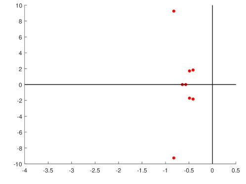
Figure 2. The closed loop eigenvalues with controller $C(s)$ in Example 8.

There are three pairs of eigenvalues in the figure two units or less away from the imaginary axis. These are the eigenvalues corresponding to the poles of $C_{r}$. They are moving to the left from the imaginary axis when increasing $\varepsilon$ from zero to $0.5$. The remaining eigenvalues shown in the figure are the rightmost eigenvalues of the stabilized closed-loop system of Step 2 that move to the right as $\varepsilon$ is increased. Thus, the stability margin obtained with the proposed choice of $\varepsilon$ is nearly optimal with the stabilizing controller constructed in Step 2. In comparison, the stability margin obtained by using the actual closed-loop transfer matrix $P$ instead of the approximated one when constructing $C_{r}$ is $0.4588$.

Finally, the closed loop system is simulated. The approximation in the simulation is obtained by using finite differences with 150 points on $[0,1]$. Fig. 3 shows the behavior of the measured outputs. As expected, the outputs converge asymptotically to the reference signals. The oscillation is mainly due to the eigenvalues with the largest imaginary parts shown in Fig. 2.

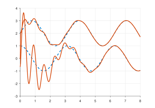
Figure 3. The measured signals (solid) and the reference signals (dashed) of Example 8.

8. Concluding Remarks

This article introduced general frequency domain theory for robust regulation using fractional representations. The main theoretical contributions were the new formulation of the internal model principle, several conditions for solvability, and the parametrization of all robustly regulating controllers. Causality considerations were included. The usefulness of the results is due to the generality assured by the minimal set of standing assumptions and not requiring the existence of coprime factorizations. Unlike the results that are related to specific rings of stable transfer functions^{21; 7}, the results presented in this article allow one to choose the stability type to work with. This is particularly important since the achievable stability type depends on the problem at hand as was demonstrated by Example 7 in which the choice of the ring of stable transfer functions was not trivial due to the challenging unstable dynamics of the reference signals.

The given conditions for solvability were accompanied by design procedures for robust controllers. Although it was not possible to give details on how to accomplish the steps of the design procedures due to the general approach, comparing the procedures reveals some main ideas. First, some of the procedures start with a step where the internal model is simplified. This step is compulsory in Design procedure 5 and is particularly important in the other procedures as well since without it the constructed internal model tends to be oversized, see Remark 12. Secondly, Design procedure 1 gives a recursive process to construct the internal model into the controller. This technique enables one to revise an existing robustly regulating controller by adding an internal model of new unstable dynamics so that it can handle a larger class of reference signals. Thirdly, a two-step approach where one first stabilizes the plant and then constructs an internal model into the controller was used in Design procedures 2-4. This may be particularly handy since finding a robust controller for a stable plant can be straightforward as was seen in Example 8. In Design procedure 5, the order of stabilization and construction of internal model was reversed. Adding the internal model first and then stabilizing the resulting system is a straightforward method, but the downside is that one needs to stabilize the unstable dynamics of the plant and the signal generator at once.

The results of this article help in understanding some of the fundamental ideas in robust regulation such as the internal model principle. Whereas the results generalize the existing ones that are specific to some rings of stable transfer functions, they now provide a good starting point to go back from general to specific. In particular, several results require finding a generating set for a specific fractional ideal or solving matrix equations such as (6) or (12). These are not easy tasks in general and an interesting direction for future research would be to find out what one can say about their solvability in some of the most general rings of stable transfer functions such as $H^{\infty}$. On the other hand, one can try to find alternative formulations of the main results in order to obtain new insights. This has been done with SISO systems using fractional ideals.³⁹ Two prominent frameworks for achieving further insights into robust regulation of MIMO systems are the lattice approach or the geometric systems theory.^{29; 45} The results concerning causality were not complete for causal plants. Therefore, stronger results on causal stabilizing controllers such as parametrization of all causal controllers would be of great interest. Parametrizations for strictly causal controllers are already available⁴⁶.

References

- [1] Oberkampf WL, DeLand SM, Rutherford BM, Diegert KV, Alvin KF. Error and uncertainty in modeling and simulation. Reliab. Eng. Syst. Saf. 2002; 75(3): 333 - 357. doi: 10.1016/S0951-8320(01)00120-X
- [2] Paunonen L, Pohjolainen S. Internal model theory for distributed parameter systems. SIAM J. Control Optim. 2010; 48(7): 4753–4775. doi: 10.1137/090760957
- [3] Ball JA, Sasane AJ. Extension of the -metric. Complex Anal. Oper. Theory 2012; 6: 65–89. doi: 10.1007/s11785-010-0097-y
- [4] Quadrat A. The homological perturbation lemma and its applications to robust stabilization. IFAC-PapersOnLine 2015; 48(14): 7–12. 8th IFAC Symposium on Robust Control Design ROCOND 2015doi: 10.1016/j.ifacol.2015.09.425
- [5] Vidyasagar M, Schneider H, Francis BA. Algebraic and topological aspects of feedback stabilization. IEEE Trans. Automat. Control 1982; 27(4): 880–894. doi: 10.1109/TAC.1982.1103015
- [6] Curtain R, Zwart HJ. An introduction to infinite-dimensional linear systems theory. Springer. 1st ed. 1995
- [7] Vidyasagar M. Control system synthesis: A factorization approach. MIT Press . 1985.
- [8] Callier FM, Desoer CA. Stabilization, tracking and disturbance rejection in multivariable convolution systems. Annales de la Société Scientifique de Bruxelles 1980; 94(I): 7–51.
- [9] Antsaklis P, Pearson J. Stabilization and regulation in linear multivariable systems. IEEE Trans. Automat. Control 1978; 23(5): 928–930. doi: 10.1109/TAC.1978.1101880
- [10] Davison EJ. The robust control of a servomechanism problem for linear time-invariant multivariable systems. IEEE Trans. Automat. Control 1976; 21(1): 25–34. doi: 10.1109/TAC.1976.1101137
- [11] Davison EJ, Goldenberg A. Robust control of a general servomechanism problem: The servo compensator. Automatica 1975; 11(5): 461–471. doi: 10.1016/0005-1098(75)90022-9
- [12] Francis BA, Wonham WM. The internal model principle of control theory. Automatica 1976; 12(5): 457–465. doi: 10.1016/0005-1098(76)90006-6
- [13] Francis B, Wonham W. The internal model principle for linear multivariable regulators. Appl. Math. Optim. 1975; 2(2): 170–194. doi: 10.1007/BF01447855
- [14] Pohjolainen SA. Robust controller for systems with exponentially stable strongly continuous semigroups. J. Math. Anal. Appl. 1985; 111(2): 622–636. doi: 10.1016/0022-247X(85)90239-2
- [15] Yamamoto Y, Hara S. Relationships between internal and external stability for infinite-dimensional systems with applications to a servo problem. IEEE Trans. Automat. Control 1988; 33(11): 1044–1052. doi: 10.1109/9.14416
- [16] Bymes CI, Lauko IG, Gilliam DS, Shubov VI. Output regulation for linear distributed parameter systems. IEEE Trans. Automat. Control 2000; 45(12): 2236-2252. doi: 10.1109/9.895561
- [17] Hämäläinen T, Pohjolainen S. A finite-dimensional robust controller for systems in the CD-Algebra. IEEE Trans. Automat. Control 2000; 45(3): 421–431. doi: 10.1109/9.847722
- [18] Rebarber R, Weiss G. Internal model based tracking and disturbance rejection for stable well-posed systems. Automatica 2003; 39(9): 1555–1569. doi: 10.1016/S0005-1098(03)00192-4
- [19] Immonen E. State space output regulation theory for infinite-dimensional linear systems and bounded uniformly continuous exogenous signals. PhD thesis. Tampere University of Technology, Tampere, Finland; 2006.
- [20] Paunonen L, Pohjolainen S. The internal model principle for systems with unbounded control and observation. SIAM J. Control Optim. 2014; 52(6): 3967-4000. doi: 10.1137/130921362
- [21] Laakkonen P, Pohjolainen S. Frequency domain robust regulation of signals generated by an infinite-dimensional exosystem. SIAM J. Control Optim. 2015; 53(1): 139–166. doi: 10.1137/130950057
- [22] Humaloja J, Kurula M, Paunonen L. Approximate robust output regulation of boundary control systems. IEEE Trans. Automat. Control 2019; 64(6): 2210-2223. doi: 10.1109/TAC.2018.2884676
- [23] Nett CN. The fractional representation approach to robust linear feedback design: A self-contained exposition. Master’s thesis. Rensselaer Polytechnic Institute. Troy, New York, USA: 1984.
- [24] Laakkonen P, Quadrat A. A fractional representation approach to the robust regulation problem for SISO systems. Syst. Control. Lett. 2017; 103: 32–37. doi: 10.1016/j.sysconle.2017.02.006
- [25] Ylinen L, Hämäläinen T, Pohjolainen S. Robust regulation of stable systems in the -algebra. Internat. J. Control 2006; 79(1): 24–35. doi: 10.1080/00207170500390903
- [26] Desoer CA, Liu RW, Murray J, Saeks R. Feedback system design: The fractional representation approach to analysis and synthesis. IEEE Trans. Automat. Control 1980; 25(3): 399–412. doi: 10.1109/TAC.1980.1102374
- [27] Logemann H. Stabilization and regulation of infinite-dimensional systems using coprime factorizations. In: Curtain R, Bensoussan A, Lions J. , eds. Analysis and optimization of systems: State and frequency domain approaches for infinite-dimensional systems. 185 of Lecture Notes in Control and Information Sciences. Springer-Verlag, Berlin. 1993 (pp. 102–139)
- [28] Pekar L, Prokop R. The revision and extension of the ring for time delay systems. Bull. Pol. Ac.: Tech. 2017; 65: 341–349. doi: 10.1515/bpasts-2017-0038
- [29] Quadrat A. On a generalization of the Youla-Kučera parametrization. Part II: The lattice approach to MIMO systems. Math. Control Signals Syst. 2006; 18(3): 199–235. doi: 10.1007/s00498-005-0160-9
- [30] Logemann H. Finitely ganerated ideals in certain algebras of transfer functions for infinite-dimensional systems. Internat. J. Control 1987; 45(1): 247–250. doi: 10.1080/00207178708933724
- [31] Laakkonen P. Robust regulation theory for transfer functions with a coprime factorization. IEEE Trans. Automat. Control 2016; 61(10): 3109–3114. doi: 10.1109/TAC.2015.2497898
- [32] Mori K, Abe K. Feedback stabilization over commutative rings: Further study of the coordinate-free approach. SIAM J. Control Optim. 2001; 39(6): 1952–1973. doi: 10.1137/S0363012998336625
- [33] Laakkonen P. Robust regulation of MIMO systems: A reformulation of the internal model principle. IFAC-PapersOnLine 2017; 50(1): 693 – 697. 20th IFAC World Congressdoi: 10.1016/j.ifacol.2017.08.125
- [34] Paunonen L, Laakkonen P. Polynomial input-output stability for linear systems. IEEE Trans. Automat. Control 2015; 60(10): 2797-2802. doi: 10.1109/TAC.2015.2398890
- [35] Oostveen J. Strongly stabilizable distributed parameter systems. Society for Industrial and Applied Mathematics . 2000
- [36] Quadrat A. A lattice approach to analysis and synthesis problems. Math. Control Signals Systems 2006; 18(2): 147–186. doi: 10.1007/s00498-005-0159-2
- [37] Sule VR. Feedback stabilization over commutative rings: The matrix case. SIAM J. Control Optim. 1994; 32(6): 1675-1695. doi: 10.1137/S036301299122027X
- [38] Francis BA, Wonham WM. The role of trasnmission zeros in linear multivariable regulators. Internat. J. Control 1975; 22(5): 657–681. doi: 10.1080/00207177508922111
- [39] Laakkonen P, Quadrat A. Robust regulation of SISO systems: The fractional ideal approach. In: Proceedings of SIAM Conference on Control & Its Applications (SIAM CT15); 2015; Paris, France: 311–318
- [40] Callier FM, Desoer CA. An algebra of transfer functions for distributed linear time-invariant systems. IEEE Trans. Circuits Syst. 1978; 25(9): 651–662. doi: 10.1109/TCS.1978.1084544
- [41] Lang S. Algebra. Springer-Verlag, New York. Revised 3rd ed. 2002.
- [42] Curtain R, Morris K. Transfer functions of distributed parameter systems: A tutorial. Automatica 2009; 45(5): 1101-1116. doi: 10.1016/j.automatica.2009.01.008
- [43] Curtain R, Salamon D. Finite-dimensional compensators for infinite-dimensional systems with unbounded input operators. SIAM J. Control Optim. 1986; 24(4): 797–816. doi: 10.1137/0324050
- [44] Oară C, Varga A. Minimal degree coprime factorization of rational matrices. SIAM J. Matrix Anal. Appl. 1999; 21(1): 245-278. doi: 10.1137/S0895479898339979
- [45] Falb P. Methods of algebraic geometry in control theory Part II: Multivariable linear systems and projective algebraic geometry. Methods of Algebraic Geometry in Control Theory. Springer Science+Business Media, New York. Softcover reprint of the original 1st ed. 1999.
- [46] Mori K. Parametrization of all strictly causal stabilizing controllers. IEEE Transactions on Automatic Control 2009; 54(9): 2211-2215. doi: 10.1109/TAC.2009.2026847