State-Switching Control of
the Second-Order Chained Form System

Abstract

This paper addresses a motion planning problem of the second-order chained form system. The author presents a novel control approach based on switching a state. The second-order chained form system is composed of three subsystems including two double integrators and a nonlinear system. Switching a single state of the double integrators can modify the nature of the nonlinear system. Such state-switching and sinusoidal control construct the basis of the proposed control approach. The effectiveness is validated by a simulation result.

1 Introduction

Nonlinear dynamical systems with non-integrable differential constraints, the so-called nonholonomic systems, have been attracting many researchers and engineers for the last three decades. A theorem in Brockett (1983) gave a challenging and negative fact that there does not exist any smooth time-invariant feedback control law to be able to stabilize nonholonomic systems. The applications include various types of robotic vehicles and manipulation. Some of them have been often used as a kind of benchmark platform to demonstrate the performance of a proposed controller for not only a control problem of a single robotic system and also a distributed control problem of multiagent robotic systems.

A V/STOL aircraft without gravity (Hauser et al. (1992)), an underactuated manipulator (Arai et al. (1998)), and an underactuated hovercraft (He et al. (2016)) belong to a class of dynamic nonholonomic systems which are subject to acceleration constraints. The mathematical representation of these systems can be transformed to the second-order chained form by a coordinate and input transformation. The second-order chained form is a canonical form for dynamic nonholonomic systems.

Several control approaches to the second-order chained-form system have been developed so far. Most of them focuses on avoiding the theorem of Brockett (1983). Ge et al. (2001) and He et al. (2016) exploit discontinuity in their stabilizing controllers; De Luca and Oriolo (2002) and Aneke et al. (2003) reduce the control problem into a trajectory tracking problem. Other than those, Yoshikawa et al. (2000) and Ito (2019) consider a motion planning problem (in other words, a feedforward control problem).

For motion planning of the second-order chained form system, this paper presents a novel control approach based on switching a state. The second-order chained form system is divided into three subsystems. Two of them are the so-called double integrators; the other subsystem is a nonlinear system depending on one of the double integrators. In other words, the input matrix of the latter subsystem depends on a single state of the double integrators. The double integrator is linearly controllable, which enables to switch the value of the position state in order to modify the nature of the nonlinear subsystem. Steering the value into one corresponds to modifying the nonlinear subsystem into the double integrator; steering the value into zero corresponds to modifying the nonlinear subsystem into a linear autonomous system. This nature is the basis of the proposed control approach. The proposed approach is composed of such state-switching and also sinusoidal control inputs. Its effectiveness is validated by a simulation result.

2 Subsystem Decomposition of the Second-Order Chained Form System

Consider the following second-order chained form system:

$$\frac{\displaystyle\mathrm{d}{}^{2}}{\displaystyle\mathrm{d}t^{2}}\boldsymbol{\xi}=\begin{bmatrix}1&0\\ 0&1\\ \xi_{2}&0\end{bmatrix}\boldsymbol{u},$$ (1)

where $\boldsymbol{\xi}:=[\,\xi_{1},\,\xi_{2},\,\xi_{3}\,]^{\top}$ and $\boldsymbol{u}=[\,u_{1},\,u_{2}\,]^{\top}$. By defining a state vector as $\boldsymbol{z}=[\,z_{1},\,\dotsc,z_{6}\,]^{\top}:=[\,\boldsymbol{\xi}^{\top},\,\dot{\boldsymbol{\xi}}^{\top}\,]^{\top}$, the system (1) is described as

$$\frac{\displaystyle\mathrm{d}}{\displaystyle\mathrm{d}t}\boldsymbol{z}=\begin{bmatrix}z_{4}\\ z_{5}\\ z_{6}\\ 0\\ 0\\ 0\end{bmatrix}+\begin{bmatrix}0\\ 0\\ 0\\ 1\\ 0\\ z_{2}\end{bmatrix}u_{1}+\begin{bmatrix}0\\ 0\\ 0\\ 0\\ 1\\ 0\end{bmatrix}u_{2}.$$ (2)

This affine nonlinear system (2) has equilibrium points at $\boldsymbol{z}_{e}:=[\,z_{1}^{\star},\,z_{2}^{\star},\,z_{3}^{\star},\>0,\,0,\,0\,]^{\top}$, $z_{1}^{\star},z_{2}^{\star},z_{3}^{\star}\in{\mathbb{R}}$ with $u_{1}=u_{2}=0$. By using the theorem of Sussmann (1987), we can easily confirm that the system (2) (or (1)) is small-time local controllable at $\boldsymbol{z}_{e}$.

From the viewpoint to separate the control inputs, the system (1) is divided into the following two subsystems:

$$\frac{\displaystyle\mathrm{d}}{\displaystyle\mathrm{d}t}\begin{bmatrix}z_{2}\\ z_{5}\end{bmatrix} =\begin{bmatrix}0&1\\ 0&0\end{bmatrix}\begin{bmatrix}z_{2}\\ z_{5}\end{bmatrix}+\begin{bmatrix}0\\ 1\end{bmatrix}u_{2},$$ (3a)

$$\frac{\displaystyle\mathrm{d}}{\displaystyle\mathrm{d}t}\begin{bmatrix}z_{1}\\ z_{3}\\ z_{4}\\ z_{6}\end{bmatrix} =\begin{bmatrix}0&0&1&0\\ 0&0&0&1\\ 0&0&0&0\\ 0&0&0&0\end{bmatrix}\begin{bmatrix}z_{1}\\ z_{3}\\ z_{4}\\ z_{6}\end{bmatrix}+\begin{bmatrix}0\\ 0\\ 1\\ z_{2}\end{bmatrix}u_{1}.$$ (3b)

The subsystem (3a) is a second-order linear system—the so-called double integrator; the subsystem (3b) looks a four-order linear system but its input matrix $\boldsymbol{b}_{2}$ depends on a state $z_{2}$. The subsystem (3b) is furthermore decomposed to the following subsystems:

$$\frac{\displaystyle\mathrm{d}}{\displaystyle\mathrm{d}t}\begin{bmatrix}z_{1}\\ z_{4}\end{bmatrix} =\begin{bmatrix}0&1\\ 0&0\end{bmatrix}\begin{bmatrix}z_{1}\\ z_{4}\end{bmatrix}+\begin{bmatrix}0\\ 1\end{bmatrix}u_{1},$$ (4a)

$$\frac{\displaystyle\mathrm{d}}{\displaystyle\mathrm{d}t}\begin{bmatrix}z_{3}\\ z_{6}\end{bmatrix} =\begin{bmatrix}0&1\\ 0&0\end{bmatrix}\begin{bmatrix}z_{3}\\ z_{6}\end{bmatrix}+\begin{bmatrix}0\\ z_{2}\end{bmatrix}u_{1}.$$ (4b)

The next section introduces the proposed control approach based on the above-mentioned subsystem decomposition.

3 State-Switching Control Approach

The section addresses a motion planning problem between equilibrium points of the second-order chained form system (1).

The author presents a control approach based on the subsystem decomposition that divides the second-order chained form system (1) into the three subsystems (3a), (4a), and (4b). The input matrix of the subsystem (4b) depends on a state of the subsystem (3a), $z_{2}$. The state $z_{2}$ can be constant by a control input $u_{2}$ because the subsystem (3a) is linear controllable.

Now let us consider that $z_{2}$ between $0$ and $1$ is switched. When $z_{2}$ is equivalent to $1$, the subsystems (4a) and (4b) are completely same under a shared control input $u_{1}$. The shared control input brings that the state differences between those controlled subsystems then depend on their values at the moment when $z_{2}$ just becomes $1$ In meanwhile, when $z_{2}$ is equivalent to $0$, the subsystem (4a) can be controlled independently of another subsystem (4b).

From this perspective, the author conceived the following basic maneuver for the above-mentioned motion planning problem:

1. Steer $z_{2}$ from any initial value to $1$ by using ${u_{1}}({t})=0,\ {u_{2}}({t})={q_{1}}({t})$;

2. Steer $z_{3}$ from any initial value to any desired value (in conjunction with it, $z_{1}$ is also driven) by using ${u_{1}}({t})={q_{2}}({t}),\ {u_{2}}({t})=0$;

3. Steer $z_{2}$ from $1$ to $0$ by using ${u_{1}}({t})=0,\ {u_{2}}({t})={q_{3}}({t})$;

4. Steer $z_{1}$ from a value to any desired value by using ${u_{1}}({t})={q_{4}}({t}),\ {u_{2}}({t})=0$;

5. Steer $z_{2}$ from $0$ to any desired value by using $u_{1}=0,\ u_{2}=q_{5}(t)$,

where $q_{i}(t)$ is an appropriate sinusoidal function in the $i$-th phase ($i=1,2,\dotsc,5$). Note that sinusoidal steering is inspired by the result of Ito (2019).

Remark 1

Some conventional approaches such as in Aneke et al. (2003) and Hably and Marchand (2014) also exploit similar (but different) subsystem decomposition. Note that those approaches focus on not motion planning but stabilizing (via trajectory tracking).

4 Numerical Example

A numerical example is shown to demonstrate the effectiveness of the proposed control approach.

Consider a motion planning problem between ${\boldsymbol{z}}({0})=[\,3,\,0.5,\,1,\;0,\,0,\,0\,]^{\top}$ and ${\boldsymbol{z}}({4T})=[\,0,\,0,\,0,\;0,\,0,\,0\,]^{\top}$. The basic maneuver is adjusted as follows:

1. Steer $z_{2}$ using from $0.5$ to $1$;

2. Steer $z_{3}$ from $1$ to $0$;

3. Steer $z_{2}$ from $1$ to $0$;

4. Steer $z_{1}$ from a resultant value in Step 2 to $0$.

To execute this procedure, the following control inputs were adopted:

$$\left\{\begin{array}[]{@{\,}ll@{\,}}{u_{1}}({t})=0\;\;\mbox{and}&\\[2.5pt] \lx@intercol\hfil\qquad{u_{2}}({t})=\phantom{-}a_{1}\omega^{2}\sin{\omega t}\lx@intercol,\quad&\mbox{for}\;\;t\in[0,T],\\[7.5pt] {u_{1}}({t})=-a_{2}\omega^{2}\sin{\omega t}&\\[2.5pt] \lx@intercol\hfil\mbox{and}\quad{u_{2}}({t})=0\lx@intercol,\quad&\mbox{for}\;\;t\in(T,2T],\\[7.5pt] {u_{1}}({t})=0\;\;\mbox{and}&\\[2.5pt] \lx@intercol\hfil{u_{2}}({t})=-a_{3}\omega^{2}\sin{\omega t}\lx@intercol,\quad&\mbox{for}\;\;t\in(2T,3T],\\[7.5pt] {u_{1}}({t})=-a_{4}\omega^{2}\sin{\omega t}&\\[2.5pt] \lx@intercol\hfil\mbox{and}\quad{u_{2}}({t})=0\lx@intercol,\quad&\mbox{for}\;\;t\in(3T,4T].\end{array}\right.$$ (5)

Figure 1 depicts a simulation result with $\omega=2\pi$, $T=1$, $a_{1}=0.5/(2\pi)$, $a_{2}=a_{3}=1/(2\pi)$, and $a_{4}=2/(2\pi)$. It is obvious that the desired motion is successfully planned. The proposed control approach, therefore, was confirmed to be useful for motion planning. The results of the conventional approaches such as in Aneke et al. (2003) and Hably and Marchand (2014) imply that the proposed approach can be (partially) combined with stabilization and trajectory tracking.

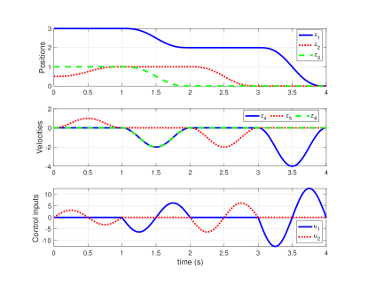
Figure 1: Time plots.

5 Conclusion

For a motion planning problem of the second-order chained form system, this paper has proposed a state-switching control approach based on subsystem decomposition. The subsystem decomposition divides the second-order chained form system to three subsystems. One of the subsystems has the input matrix that depends on a state of the other subsystem. Switching the state between one and zero modifies the nature of the associated subsystem. This is the key point of the proposed control approach. The effectiveness of the proposed approach was shown by the simulation result.

Future directions of this study are:

• to compare the proposed approach with the other related ones;

• to investigate further properties of the proposed approach; and

• to extend the second-order chained form system into the higher-order one.

References

- Aneke et al. (2003) Aneke, N.P.I., Nijmeijer, H., and de Jager, A.G. (2003). Tracking control of second-order chained form systems by cascaded backstepping. Int. J. Robust and Nonlinear Contr., 13(2), 95–115.
- Arai et al. (1998) Arai, H., Tanie, K., and Shiroma, N. (1998). Nonholonomic control of a three-DOF planar underactuated manipulator. IEEE Trans. Robot. Autom., 14(5), 681–695.
- Brockett (1983) Brockett, R.W. (1983). Asymptotic stability and feedback stabilization. In R.W. Brockett, R.S. Millmann, and H.J. Sussmann (eds.), Differential Geometric Control Theory, 181–191. Birkhauser.
- De Luca and Oriolo (2002) De Luca, A. and Oriolo, G. (2002). Trajectory planning and control for planar robots with passive last joint. Int. J. Robot. Res., 21(5–6), 575–590.
- Ge et al. (2001) Ge, S.S., Sun, Z., Lee, T.H., and Spong, M.W. (2001). Feedback linearization and stabilization of second-order nonholonomic chained systems. Int. J. Contr., 74(14), 1383–1392.
- Hably and Marchand (2014) Hably, A. and Marchand, N. (2014). Bounded control of a general extended chained form systems. In In Proc. 53rd IEEE Conf. Decis. Contr., 6342–6347.
- Hauser et al. (1992) Hauser, J., Sastry, S., and Meyer, G. (1992). Nonlinear control design for slightly non-minimum phase systems: applicatio to V/STOL aircraft. Automatica, 28(4), 665–679.
- He et al. (2016) He, G., Zhang, C., Sun, W., and Geng, Z. (2016). Stabilizing the second-order nonholonomic systems with chained form by finite-time stabilizing controllers. Robotica, 34, 2344–2367.
- Ito (2019) Ito, M. (2019). Motion planning of a second-order nonholonomic chained form system based on holonomy extraction. Electronics, 8(11), 1337.
- Sussmann (1987) Sussmann, H.J. (1987). A general theorem on local controllability. SIAM J. Contr. Optim., 25(1), 158–194.
- Yoshikawa et al. (2000) Yoshikawa, T., Kobayashi, K., and Watanabe, T. (2000). Design of a desirable trajectory and convergent control for 3-D.O.F manipulator with a nonholonomic constraint. In Proc. IEEE Int. Conf. Robot. Autom., 1805–1810.