On the Distance of SGR 1935+2154 Associated with FRB 200428 and Hosted in SNR G57.2+0.8

Abstract

Owing to the detection of an extremely bright fast radio burst (FRB) 200428 associated with a hard X-ray counterpart from the magnetar soft gamma-ray repeater (SGR) 1935+2154, the distance of SGR 1935+2154 potentially hosted in the supernova remnant (SNR) G57.2+0.8 can be revisited. Under the assumption that the SGR and the SNR are physically related, in this Letter, by investigating the dispersion measure (DM) of the FRB contributed by the foreground medium of our Galaxy and the local environments and combining with other observational constraints, we find that the distance of SGR 1935+2154 turns out to be $9.0\pm 2.5\,$kpc and the SNR radius falls into $10$ to $18\,$pc since the local DM contribution is as low as $0-18\,$pc cm^-3. These results are basically consistent with the previous studies. In addition, an estimate for the Faraday rotation measure of the SGR and SNR is also carried out.

1 Introduction

Very recently, an extremely bright millisecond-timescale radio burst from the Galactic magnetar SGR 1935+2154 was reported by The CHIME/FRB Collaboration et al. (2020) and Bochenek et al. (2020). More excitingly, its associated X-ray burst counterpart was also detected by Insight-HXMT (Zhang et al., 2020b, c, d; Li et al., 2020), AGILE (Tavani et al., 2020), INTEGRAL (Mereghetti et al., 2020), and Konus-Wind (Ridnaia et al., 2020) telescopes. Additionally, a subsequent highly polarised transient pulsating radio burst was detected by the FAST radio telescope with Faraday rotation measure (RM) +112.3 rad m^-2 (Zhang et al., 2020a), consistent with RM$=+116\pm 6$ rad m^-2 of FRB 200428 (The CHIME/FRB Collaboration et al., 2020). From the previous investigations about the magnetar SGR 1935+2154, we know that it has a spin period $P\simeq 3.24$ s, a spin-down rate ${\dot{P}}\simeq 1.43\times 10^{-11}\,{\rm s}\,{\rm s}^{-1}$, a surface dipole magnetic field strength $B_{\rm p}\simeq 2.2\times 10^{14}~{}{\rm G}$, an age $t\sim 3.6$ kyr, and a spin-down luminosity $L_{\rm sd}\sim 1.7\times 10^{34}\ \rm{erg~{}s}^{-1}$ (Israel et al., 2016), hosted in the Galactic supernova remnant (SNR) G57.2+0.8 with a high probability (Gaensler, 2014).

In the literature, however, the distance of SNR G57.2+0.8 has a large range and remains highly debated even though various methods have been used, e.g., the statistical radio surface-brightness-to-diameter relation ($\sim 9.1$ kpc, Pavlović et al., 2013), the empirical relation between the HI column density $N_{\rm H}$ and the dispersion measure (DM) ($11.7\pm 2.8$ kpc, Surnis et al., 2016), and the local standard of rest (LSR) velocity measure via HI absorption feature ($12.5\pm 1.5$ kpc, Kothes et al., 2018), ($4.5-9.0$ kpc, Ranasinghe et al., 2018), or via CO gas towards the SNR ($6.6\pm 0.7$ kpc, Zhou et al., 2020). For SGR 1935+2154, Kozlova et al. (2016) gave an upper limit $<10$ kpc through the scattered correlation between the squares of the radii of the emitting areas and the corresponding black-body temperatures, and Mereghetti et al. (2020) obtained $2.2-7.1$ kpc through the observation of the bright dust-scattering X-ray ring. Note that the methods tracing the SNR are radio-based only and those tracing the SGR are X-ray-based only. Due to the position of the SGR at the geometric center of the SNR in a relatively uncrowded region of the Galactic plane (Gaensler, 2014), to the distance estimates and approximate ages inferred for the SGR and the SNR, it is believed that they are likely physically related (Kothes et al., 2018). Moreover, the relatively small age (3.6 kyr) of the SGR supports that its SNR should be visible (Zhou et al., 2020). All these pieces of evidence strongly suggest a likely association between the SGR and the SNR.

In this Letter, we therefore assume that SGR 1935+2154 is indeed associated with SNR G57.2+0.8 and the SNR has the same age as the SGR, and then use DM by combining with other observational constraints to estimate the distance of the SGR in Section 2. Our results are displayed in Section 3. A discussion on RM estimate is arranged in Section 4, and conclusions are drawn in Section 5.

2 DM Estimate

The CHIME/FRB Collaboration et al. (2020) and Bochenek et al. (2020) reported that FRB 200428 has an observed DM${}_{\rm obs}=332.7$ pc cm^-3. The DM_obs is mainly contributed by the foreground interstellar medium (ISM) in our Galaxy (DM_Gal), the magnetar wind nebula (DM_MWN), and the SNR (DM_SNR), that is,

$${\rm DM_{obs}=DM_{Gal}+DM_{MWN}+DM_{SNR}},$$ (1)

where the foreground DM of our Galaxy is

$${\rm DM_{Gal}}=\int_{0}^{D}n_{e}(l)dl,$$ (2)

related to the distance $D$ of SGR 1935+2154 via the Galactic electron density ($n_{e}$) distribution NE2001 (Cordes & Lazio, 2002, 2003) or YMW16 (Yao et al., 2017).

The DM_MWN is primarily attributed to O-mode wave and may be given by (e.g., Yu, 2014; Cao et al., 2017; Yang & Zhang, 2017)

$$\mathrm{DM}_{\rm MWN}\simeq 0.082\ \rm{pc}\ \rm{cm}^{-3}\ \mu_{\pm,4}^{2/3}B_{\rm p,14}^{4/3}P_{0}^{-11/3},$$ (3)

where $\mu_{\pm}=10^{4}\mu_{\pm,4}$ is the multiplicity parameter of the electron-positron pairs, $B_{\rm p}=10^{14}B_{\rm p,14}$ G and $P=10^{0}P_{0}$ s are the dipole magnetic field and the rotation period of the magnetar, respectively.

In regard to the DM_SNR, it depends on ambient medium: constant density ISM or wind environment. So we consider the DM contribution by the SNR in two different scenarios as follows.

2.1 Constant ISM

It is widely accepted that an SNR has three phases after a supernova (SN) explosion in constant ISM scenario: (a) the free-expansion phase, (b) the Sedov-Taylor phase, and (c) the snowplow phase. Because SNR G57.2+0.8 has possibly reached the end of the Sedov-Taylor phase or entered the snowplow phase due to the non-detection of X-ray emission (Kothes et al., 2018; Zhou et al., 2020), the DM_SNR from the ionized medium (including shocked SN ejecta and shocked swept ambient medium), can be estimated by

$${\rm DM_{SNR}}\simeq\left\{\begin{array}[]{ll}34\ {\rm pc\ cm^{-3}}\ t_{2}^{2/5}E_{51}^{1/5}n_{2}^{4/5},&t<t_{\rm SP}\\ 81\ {\rm pc\ cm^{-3}}\ t_{3}^{2/7}E_{51}^{0.225}n_{2}^{0.737},&t>t_{\rm SP}\end{array}\right.$$ (4)

during the Sedov-Taylor and snowplow phases (e.g., Yang & Zhang, 2017; Piro & Gaensler, 2018), where $t=10^{i}t_{i}$ yr is the age of the SNR, $E=10^{51}E_{51}$ erg is the energy of the SN explosion, and $n=10^{2}n_{2}$ cm^-3 is the number density of a uniform ISM, as well as the snowplow time $t_{\rm SP}\simeq 3920\ {\rm yr}\ E_{51}^{0.22}n_{2}^{-0.55}$ (e.g., Draine, 2011). The corresponding SNR radius can be written by (e.g., Taylor, 1950; Sedov, 1959; Draine, 2011; Yang & Zhang, 2017)

$$R_{\rm SNR}\simeq\left\{\begin{array}[]{ll}0.84\ {\rm pc}\ t_{2}^{2/5}E_{51}^{1/5}n_{2}^{-1/5},&t<t_{\rm SP}\\ 2.44\ {\rm pc}\ t_{3}^{2/7}E_{51}^{0.225}n_{2}^{-0.263},&t>t_{\rm SP}\end{array}\right.$$ (5)

where we have used the Sedov-Taylor radius independent of the mass of the SN ejecta as the SNR radius (Yang & Zhang, 2017) rather than the blastwave radius depending on the mass of the SN ejecta (Piro & Gaensler, 2018), because the Sedov-Taylor radius can be a good representation of the SNR radius when the SNR has been well past the free-expansion phase.

2.2 Wind Environment

In a wind environment, the SNR evolution has two phases: the early ejecta-dominated phase and the very late wind-dominated phase, based on Piro & Gaensler (2018). During these phases, the DM_SNR is calculated by (see Table 2 of Piro & Gaensler, 2018)

$${\rm DM_{SNR}}\simeq\left\{\begin{array}[]{ll}13\ {\rm pc\ cm^{-3}}\ \mu_{e}^{-1}t_{2}^{-3/2}E_{51}^{-3/4}M_{1}^{5/4}K_{13}^{1/2},&\\ t<t_{\rm ch}\\ 0.088\ {\rm pc\ cm^{-3}}\ \mu_{e}^{-1}t_{3}^{-2/3}E_{51}^{-1/3}K_{13}^{4/3},&\\ t>t_{\rm ch}\end{array}\right.$$ (6)

where $\mu_{e}$ is the mean molecular weight per electron, $M=M_{1}\times 1M_{\odot}$ is the mass of the SN ejecta, $K=5.1\times 10^{13}\ {\rm g~{}cm}^{-1}\ \dot{M}_{-5}{v}_{6}^{-1}$ (here the mass-loss rate $\dot{M}_{-5}=10^{-5}M_{\odot}\ \rm{yr}^{-1}$ and the wind velocity $v_{6}=v_{w}/10^{6}\ \rm{cm}\ \rm{s}^{-1}$), and the characteristic time $t_{\rm{ch}}=1.9\times 10^{3}\ {\rm yr}\ E_{51}^{-1/2}M_{1}^{3/2}K_{13}^{-1}$ separating these phases. This characteristic time corresponds to a radius $R_{\rm{ch}}=16.8\ {\rm pc}\ M_{1}K_{13}^{-1}$. Please note that the SNR radius deemed as the blastwave radius can be linked to $R_{\rm ch}$ and $t_{\rm ch}$ through the analytic functions (see Table 2 of Piro & Gaensler, 2018)

$$R_{\rm SNR}\simeq\left\{\begin{array}[]{ll}1.79R_{\rm ch}\left(t/t_{\rm{ch}}\right)\left[1+0.33\left(t/t_{\rm{ch}}\right)^{1/2}\right]^{-2},&\\ t<t_{\rm ch}\\ \left[1.11\left(t/t_{\rm{ch}}\right)-0.11\right]^{2/3}R_{\rm ch},&\\ t>t_{\rm ch}.\end{array}\right.$$ (7)

3 DM Results

A useful observational constraint for SNR G57.2+0.8 is that it is an almost circular source with an average diameter about $10^{\prime}$, i.e., radius $\theta_{\rm r}\approx 5^{\prime}.5$ (Kothes et al., 2018), which is relevant to the SNR radius via the distance of SGR 1935+2154

$$D=\frac{R_{\rm SNR}}{\theta_{\rm r}}.$$ (8)

Likewise, the observational constraints for ${\rm DM_{obs}}$, $t$, $B_{\rm p}$, and $P$ are also known. Through the calculation of Equation (3), we find that the value of ${\rm DM_{MWN}}$ is far smaller than 1 pc cm^-3 even if $\mu_{\pm}$ is very large like $10^{6}$, so we safely ignore this term in Equation (1) for subsequent calculations.

In the ISM scenario for the SNR, utilizing Equations (1), (2), (4), (5), and (8), one gets a power-law relation with an index 1.0 between the explosion energy $E$ and the ambient medium density $n$ (using parameter values $\theta_{\rm r}\approx 5^{\prime}.5$, ${\rm DM_{obs}}=332.7$ pc cm^-3, and $t=3.6$ kyr), as illustrated in the top panel of Figure 1. Furthermore, it is obvious that the ambient medium density has a relatively small value, i.e., $<5$ cm^-3, within a typical explosion energy ranging from several $10^{49}$ erg to several $10^{51}$ erg (e.g., Pejcha & Prieto, 2015; Lyman et al., 2016). Meanwhile, one can also acquire a distance distribution $D\simeq 6.5-11.5$ kpc with a mean value 9.0 kpc (so the SNR radius $R_{\rm SNR}\simeq 10-18$ pc), and a DM distribution of the SNR ${\rm DM_{SNR}}\simeq 0-18$ pc cm^-3 illustrating in the middle and bottom panels of Figure 1. Obviously, the DM_SNR is very low, compared with the Galactic contribution DM_Cal. Note that we have considered the uncertainty for the distance estimate via YMW16 model throughout the numerical calculations since it is the main uncertainty. As shown in Table 4 of Yao et al. (2017), the direction of SGR 1935+2154 is closest to that of the pulsar J1932+2220 with a relative uncertainty $D_{\rm err}\sim 26\%$ for the distance estimate, thus the distance of SGR 1935+2154 could also have a relative uncertainty $\sim 26\%$. The lines in Figure 1 represent the numerical results without considering the uncertainty for the distance. In reality, it is easy to roughly check these numerical results such as $E\propto n$ via DM${}_{\rm obs}\propto\,\,$DM${}_{\rm Gal}\propto D\propto R_{\rm SNR}\propto E^{1/5}n^{-1/5}$ for $t<t_{\rm SP}$ when DM_obs is dominated by DM_Gal.

For a wind environment towards the SNR, employing Equations (1), (2), (6), (7), and (8), one obtains a relation between the explosion energy $E$ and the parameter $K$ for $M=2~{}M_{\odot}$ (stripped-envelope SNe) and $M=10~{}M_{\odot}$ (red supergiant progenitors), as shown in the top panel of Figure 2. The parameter $K$ declines sharply when the explosion energy $E<6\times 10^{50}$ erg ($E<3\times 10^{51}$ erg) for $M=2M_{\odot}$ ($M=10M_{\odot}$), so we calculate the numerical results by only considering the explosion energy $E>6\times 10^{50}$ erg ($E>3\times 10^{51}$ erg) for $M=2M_{\odot}$ ($M=10M_{\odot}$). The remaining panels of Figure 2 show that the distance spans $D\simeq 6.5-11.5$ kpc and the DM contribution of the SNR occupies DM${}_{\rm SNR}\simeq 0-18$ pc cm^-3 for both $M=2M_{\odot}$ and $M=10M_{\odot}$. These results are in good agreement with those in the ISM scenario.

In summary, our results generally agree with those in the previous studies by Pavlović et al. (2013), Surnis et al. (2016), Kothes et al. (2018), Ranasinghe et al. (2018), and Zhou et al. (2020) for SNR G57.2+0.8, and Kozlova et al. (2016) and Mereghetti et al. (2020) for SGR 1935+2154. The methods in Pavlović et al. (2013), Surnis et al. (2016), and Kozlova et al. (2016) are empirical and statistical, with intrinsic large scatter. Those methods in Kothes et al. (2018), Ranasinghe et al. (2018), and Zhou et al. (2020) seem to be relevant to direct measurements and their uncertainties mainly stem from the LSR velocity measure and the rotation curve of the Galaxy. While the uncertainties in the method of Mereghetti et al. (2020) may result mostly from the determination of the dust layer and the dust-scattering distance. In comparison, the distance estimate from DM in this Letter is assumption-dependent and model-dependent though, the results are not variable for different ambient environments. The uncertainty in this method primarily originates from the Galatic electron density distribution of YMW16 model, i.e., leading to a relative uncertainty $D_{\rm err}\sim 26\%$ for the distance in the direction of SGR 1935+2154.

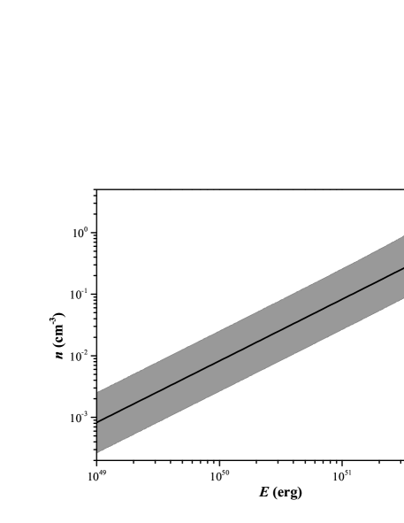
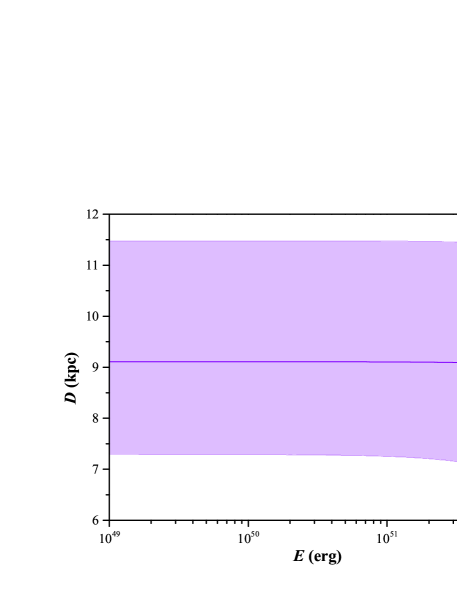
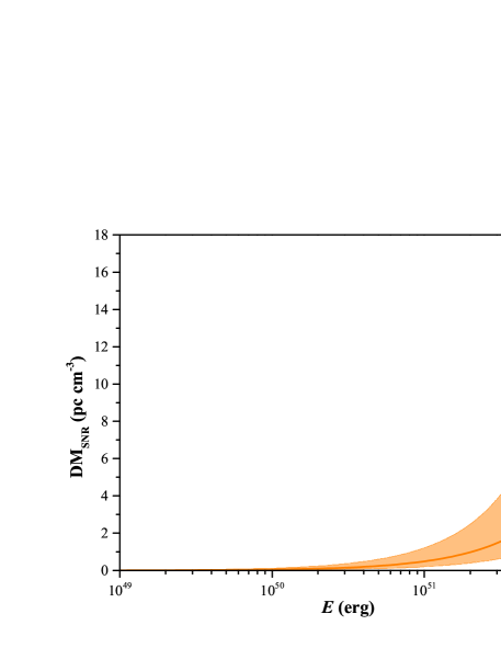
Figure 1: In a constant ISM for the SNR: (a) ambient medium density $n$ as a power-law function of energy of SN explosion $E$ (top panel); (b) the distance $D$ of SGR 1935+2154 is varied with energy of SN explosion $E$ (middle panel); (c) DM_SNR vs. explosion energy $E$ (bottom panel). The lines in three panels represent the results without considering the uncertainty for the distance estimate via YMW16 model.

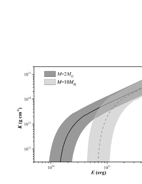
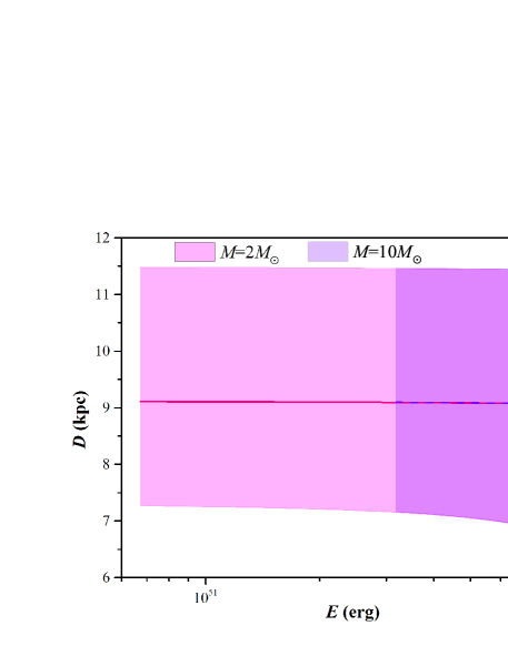
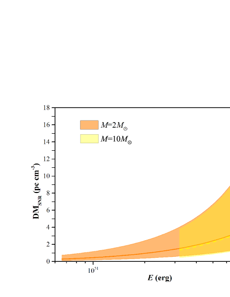
Figure 2: In a wind environment for the SNR: (a) the parameter $K=5.1\times 10^{13}\ {\rm g~{}cm}^{-1}\ \dot{M}_{-5}{v}_{6}^{-1}$ as a function of energy of SN explosion $E$ (top panel); (b) same as the middle panel of Figure 1 (middle panel); (c) same as the bottom panel of Figure 1 (bottom panel). The lines are also same as Figure 1.

4 RM Estimate

Similar to the DM estimate, the observed RM_obs should also have three parts: the foreground RM_Gal due to the Galatic ISM and permeating magnetic fields, the RM_MWN contributed by the magnetar wind nebula, and the RM_SNR resulting from the SNR, that is,

$${\rm RM_{obs}=RM_{Gal}+RM_{MWN}+RM_{SNR}}.$$ (9)

(1) The first part RM_Gal can be expressed as

$$\mathrm{RM_{Gal}}[{\rm rad~{}m^{-2}}]=0.81\int_{0}^{D}n_{\mathrm{e}}[{\rm cm^{-3}}]B_{\|}[{\rm\mu G}]dl[{\rm pc}]$$ (10)

where $B_{\|}$ is the component of the Galatic magnetic field (GMF) parallel to the line of sight. RM is positive when the magnetic field points towards us. There is a general model of the GMF consisting of two different components: a disk field and a halo field (Prouza & Šmída, 2003; Sun et al., 2008). The widely used disk field is the logarithmic spiral disk GMF model, which has two versions: the axisymmetric disk field (ASS model) and the bisymmetric disk field (BSS model) (e.g., Simard-Normandin & Kronberg, 1980; Han & Qiao, 1994; Stanev, 1997; Tinyakov & Tkachev, 2002). To estimate the RM_Gal, we consider the disk field with an ASS or BSS form and halo field with a basic form (Prouza & Šmída, 2003; Sun et al., 2008; Jansson et al., 2009; Sun & Reich, 2010; Pshirkov et al., 2011) as done in Lin & Dai (2016), combining with the Galatic free electron distribution $n_{e}$ in Yao et al. (2017) and the distance from above DM estimate. However, the RM_Gal has very different values in different models or in same models but with different parameters, from a few negative hundred to a few hundred rad m^-2 within a distance range of $D\simeq 6.5-11.5$ kpc, e.g., $\sim 470-750$ rad m^-2 for ASS+halo and $\sim 50-320$ rad m^-2 for BSS+halo in Pshirkov et al. (2011), and $\sim-220-40$ rad m^-2 for ASS+halo in Sun et al. (2008). As a result, it cannot be well evaluated by the GMF models. Nevertheless, Kothes et al. (2018) found that the foreground RM$=+223\pm 2$ rad m^-2 for SNR G57.2+0.8 via the polarized intensity maps.

(2) The second part RM_MWN arises from the magnetar wind nebula due to the magnetar spin-down energy release. The magnetic field of the nebula at time $t$ can be crudely estimated by (Metzger et al., 2017)

$$B_{\mathrm{n}}\simeq\left(\frac{6\epsilon_{B}L_{\mathrm{sd}}t}{R_{\mathrm{n}}^{3}}\right)^{1/2},$$ (11)

where $\epsilon_{B}$ is the ratio of the magnetic energy to the shock energy. Assuming $R_{\rm n}\sim(0.01-0.1)R_{\rm SNR}\simeq 0.1-2$ pc, and giving $\epsilon_{B}\sim 0.1$, $L_{\rm{sd}}\sim 1.7\times 10^{34}~{}\rm{erg~{}s}^{-1}$, and $t\sim 3.6$ kyr, one would get $B_{\rm n}\sim 0.5-100\mu{\rm G}$. In this case, a very low ${\rm{RM_{MWN}}}\simeq 0.81\ {\rm rad~{}m^{-2}}\ \frac{\rm{DM_{MWN}}}{\rm pc~{}cm^{-3}}\frac{B_{\rm n}}{\mu{\rm G}}\sim 0.005-0.3\ {\rm rad~{}m^{-2}}$ is acquired through Equation (3). Although some parameters are uncertain, the RM_MWN should be low if they fall into reasonable ranges.

(3) Akin to DM_SNR estimate, RM_SNR in different surrounding environments should have different evolutions.

ISM Scenario. In the snowplow phase, the SNR velocity is (Yang & Zhang, 2017)

$$v_{\mathrm{SP}}=690\ \mathrm{km}\ \mathrm{s}^{-1}\ t_{3}^{-5/7}E_{51}^{0.445}n_{2}^{-0.813},$$ (12)

so that the magnetic field generated in the shocked ISM is estimated by (Piro & Gaensler, 2018)

$$B_{\mathrm{ISM}} \approx \left(16\pi\epsilon m_{p}n\right)^{1/2}v_{\rm SP}$$ (13)

$$\approx 2.02\times 10^{3}\ {\rm\mu G}\ \epsilon_{-1}^{1/2}t_{3}^{-5/7}E_{51}^{0.445}n_{2}^{-0.313},$$

where $\epsilon=10^{-1}\epsilon_{-1}$ is the ratio of the magnetic energy to the shock energy. Hence, the RM_SNR in the snowplow phase ($t>t_{\rm SP}$) deduced from Equations (4) and (13) can be written down as, along with the RM_SNR in the Sedov-Taylor phase ($t<t_{\rm SP}$) (see Piro & Gaensler, 2018),

$${\rm RM_{SNR}}\simeq\left\{\begin{array}[]{ll}1.28\times 10^{5}\ {\rm rad~{}m}^{-2}\ \epsilon_{-1}^{1/2}t_{3}^{-1/5}E_{51}^{2/5}n_{2}^{11/10},&\\ t<t_{\rm SP}\\ 4.94\times 10^{4}\ {\rm rad~{}m}^{-2}\ \epsilon_{-1}^{1/2}t_{4}^{-3/7}E_{51}^{0.67}n_{2}^{0.424},&\\ t>t_{\rm SP}.\end{array}\right.$$ (14)

Combining with the relation between the energy of the SN explosion $E$ and the number density $n$ of ambient ISM in the top panel of Figure 1, one can derive RM_SNR as a power-law function of the explosion energy with an index 1.5, as displayed in the upper panel of Figure 3. It is also shown that RM_SNR can increase up to $10^{4}$ rad m^-2 when $E$ approaches to $10^{52}$ erg.

Wind Scenario. The RM_SNR in a wind environment is calculated by (Piro & Gaensler, 2018)

$${\rm RM_{SNR}}\simeq\left\{\begin{array}[]{ll}0.002\ {\rm rad~{}m}^{-2}\ x_{0.1}R_{*,2}B_{*,0}\mu_{e}^{-1}E_{51}^{-1}M_{1}t_{3}^{-2},&\\ t<t_{\rm ch}\\ 0.0017\ {\rm rad~{}m}^{-2}\ x_{0.1}R_{*,2}B_{*,0}\mu_{e}^{-1}E_{51}^{-2/3}K_{13}^{5/3}t_{4}^{-4/3},&\\ t>t_{\rm ch}\end{array}\right.$$ (15)

where $x\equiv v_{\rm rot}/v_{\rm w}$ ($v_{\rm rot}$ and $v_{\rm w}$ are the rotation velocity and wind velocity), $R_{*}=100R_{\odot}R_{*,2}$ and $B_{*}=10^{0}B_{*,0}$ G are the progenitor’s radius and magnetic field, respectively. Fixing $x=0.1$, $R_{*}=100R_{\odot}$, $\mu_{e}=1$, and $B_{*}=1$ G (even if they should be variable for different types of progenitors), and using the relation between the energy of the SN explosion $E$ and the parameter $K$ in the top panel of Figure 2 for different progenitors ($M=2M_{\odot}$ or $M=10M_{\odot}$), one gains a low RM${}_{\rm SNR}<8$ rad m^-2 when the explosion energy $E<10^{52}$ erg, as exhibited in the lower panel of Figure 3.

Notice that there are a foreground RM$=+223\pm 2$ rad m^-2 for SNR G57.2+0.8 (Kothes et al., 2018) and a RM$=+112.3$ rad m^-2 for the highly polarised radio burst from SGR 1935+2154 (Zhang et al., 2020a). If this foreground RM has no contribution from the local environment of the SNR, it would indicate that RM${}_{\rm SNR}\sim-110$ rad m^-2, corresponding to an explosion energy $E\sim(1-5)\times 10^{51}$ erg in the ISM scenario from the upper panel of Figure 3.

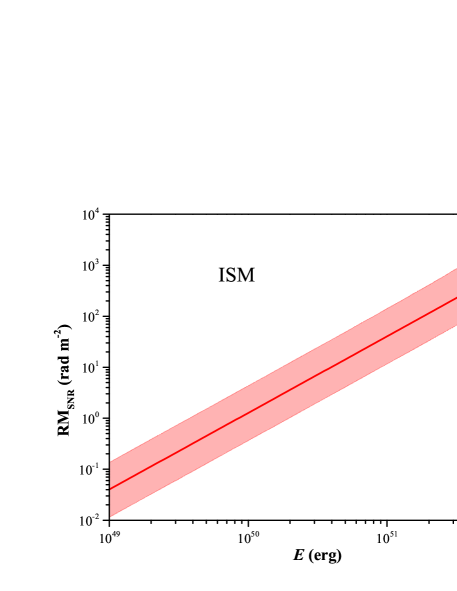
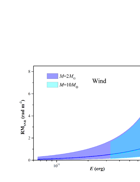
Figure 3: RM_SNR vs. energy of explosion $E$ in ISM (upper panel) and wind (lower panel) environments. The lines are same as Figure 1.

5 Conclusions

In this Letter, we have utilized DMs contributed by the foreground ISM of our Galaxy and the local environments including the magnetar wind nebula and SNR to estimate the distance of SGR 1935+2154 potentially hosted in SNR G57.2+0.8, by assuming that the SGR and the SNR are indeed associated and combining with other observational constraints. Besides, the RM estimate and relevant results have been also discussed. Some interesting results are summarized as follows:

• In the constant ISM scenario for the SNR, the energy of the SN explosion $E$ is described by a power-law function as a function of the ambient medium density $n$ with an index 1.0. Moreover, the distance, SNR radius, and DM contribution by the SNR are $D\simeq 6.5-11.5$ kpc, $R_{\rm SNR}\simeq 10-18$ pc, and ${\rm DM_{SNR}}\simeq 0-18$ pc cm^-3 within a typical range of the explosion energy, respectively.

• In the wind scenario for the SNR, the distance, SNR radius, and DM_SNR also spread over similar ranges of those in the ISM scenario for different mass of the SN ejecta.

• For the RM estimate, the polarization observations from the radio burst of the SGR and the intensity maps of the SNR might signify that the RM contribution by the local environment of the SNR is about $-110$ rad m^-2 with respect to the explosion energy $\sim(1-5)\times 10^{51}$ erg in the ISM scenario for the SNR.

Overall, our results relevant to the distance estimate are basically in agreement with the previous studies.

References

- Bochenek et al. (2020) Bochenek, C. D., Ravi, V., Belov, K. V., et al. 2020, arXiv e-prints, arXiv:2005.10828. https://arxiv.org/abs/2005.10828
- Cao et al. (2017) Cao, X.-F., Yu, Y.-W., & Dai, Z.-G. 2017, ApJ, 839, L20, doi: 10.3847/2041-8213/aa6af2
- Cordes & Lazio (2002) Cordes, J. M., & Lazio, T. J. W. 2002, arXiv e-prints, astro. https://arxiv.org/abs/astro-ph/0207156
- Cordes & Lazio (2003) —. 2003, arXiv e-prints, astro. https://arxiv.org/abs/astro-ph/0301598
- Draine (2011) Draine, B. T. 2011, Physics of the Interstellar and Intergalactic Medium (Princeton, NJ: Princeton Univ. Press)
- Gaensler (2014) Gaensler, B. M. 2014, GRB Coordinates Network, 16533, 1
- Han & Qiao (1994) Han, J. L., & Qiao, G. J. 1994, A&A, 288, 759
- Israel et al. (2016) Israel, G. L., Esposito, P., Rea, N., et al. 2016, MNRAS, 457, 3448, doi: 10.1093/mnras/stw008
- Jansson et al. (2009) Jansson, R., Farrar, G. R., Waelkens, A. H., & Enßlin, T. A. 2009, J. Cosmology Astropart. Phys, 2009, 021, doi: 10.1088/1475-7516/2009/07/021
- Kothes et al. (2018) Kothes, R., Sun, X., Gaensler, B., & Reich, W. 2018, ApJ, 852, 54, doi: 10.3847/1538-4357/aa9e89
- Kozlova et al. (2016) Kozlova, A. V., Israel, G. L., Svinkin, D. S., et al. 2016, MNRAS, 460, 2008, doi: 10.1093/mnras/stw1109
- Li et al. (2020) Li, C. K., Lin, L., Xiong, S. L., et al. 2020, arXiv e-prints, arXiv:2005.11071. https://arxiv.org/abs/2005.11071
- Lin & Dai (2016) Lin, W.-L., & Dai, Z.-G. 2016, Research in Astronomy and Astrophysics, 16, 38, doi: 10.1088/1674-4527/16/3/038
- Lyman et al. (2016) Lyman, J. D., Bersier, D., James, P. A., et al. 2016, MNRAS, 457, 328, doi: 10.1093/mnras/stv2983
- Mereghetti et al. (2020) Mereghetti, S., Savchenko, V., Ferrigno, C., et al. 2020, arXiv e-prints, arXiv:2005.06335. https://arxiv.org/abs/2005.06335
- Metzger et al. (2017) Metzger, B. D., Berger, E., & Margalit, B. 2017, ApJ, 841, 14, doi: 10.3847/1538-4357/aa633d
- Pavlović et al. (2013) Pavlović, M. Z., Urošević, D., Vukotić, B., Arbutina, B., & Göker, Ü. D. 2013, ApJS, 204, 4, doi: 10.1088/0067-0049/204/1/4
- Pejcha & Prieto (2015) Pejcha, O., & Prieto, J. L. 2015, ApJ, 806, 225, doi: 10.1088/0004-637X/806/2/225
- Piro & Gaensler (2018) Piro, A. L., & Gaensler, B. M. 2018, ApJ, 861, 150, doi: 10.3847/1538-4357/aac9bc
- Prouza & Šmída (2003) Prouza, M., & Šmída, R. 2003, A&A, 410, 1, doi: 10.1051/0004-6361:20031281
- Pshirkov et al. (2011) Pshirkov, M. S., Tinyakov, P. G., Kronberg, P. P., & Newton-McGee, K. J. 2011, ApJ, 738, 192, doi: 10.1088/0004-637X/738/2/192
- Ranasinghe et al. (2018) Ranasinghe, S., Leahy, D. A., & Tian, W. 2018, Open Physics Journal, 4, 1, doi: 10.2174/1874843001804010001
- Ridnaia et al. (2020) Ridnaia, A., Svinkin, D., Frederiks, D., et al. 2020, arXiv e-prints, arXiv:2005.11178. https://arxiv.org/abs/2005.11178
- Sedov (1959) Sedov, L. I. 1959, Similarity and Dimensional Methods in Mechanics (New York: Academic Press)
- Simard-Normandin & Kronberg (1980) Simard-Normandin, M., & Kronberg, P. P. 1980, ApJ, 242, 74, doi: 10.1086/158445
- Stanev (1997) Stanev, T. 1997, ApJ, 479, 290, doi: 10.1086/303866
- Sun & Reich (2010) Sun, X.-H., & Reich, W. 2010, Research in Astronomy and Astrophysics, 10, 1287, doi: 10.1088/1674-4527/10/12/009
- Sun et al. (2008) Sun, X. H., Reich, W., Waelkens, A., & Enßlin, T. A. 2008, A&A, 477, 573, doi: 10.1051/0004-6361:20078671
- Surnis et al. (2016) Surnis, M. P., Joshi, B. C., Maan, Y., et al. 2016, ApJ, 826, 184, doi: 10.3847/0004-637X/826/2/184
- Tavani et al. (2020) Tavani, M., Casentini, C., Ursi, A., et al. 2020, arXiv e-prints, arXiv:2005.12164. https://arxiv.org/abs/2005.12164
- Taylor (1950) Taylor, G. 1950, Proceedings of the Royal Society of London Series A, 201, 159, doi: 10.1098/rspa.1950.0049