A new study of the spectroscopic binary 7 Vul with a Be star primary

We confirmed the binary nature of the Be star 7 Vul, derived a more accurate spectroscopic orbit with an orbital period of $69\aas@@fstack{d}4212\pm 0\aas@@fstack{d}0034,$ and improved the knowledge of the basic physical elements of the system. Analyzing available photometry and the strength of the H$\alpha$ emission, we also document the long-term spectral variations of the Be primary. In addition, we confirmed rapid light changes with a period of 0$\aas@@fstack{d}$5592, which is comparable to the expected rotational period of the Be primary, but note that its amplitude and possibly its period vary with time. We were able to disentangle only the He i 6678 Å line of the secondary, which could support our tentative conclusion that the secondary appears to be a hot subdwarf. A search for this object in high-dispersion far-UV spectra could provide confirmation. Probable masses of the binary components are ($6\pm 1$) $\mathcal{M}^{\mathrm{N}}_{\odot}$ and ($0.6\pm 0.1$) $\mathcal{M}^{\mathrm{N}}_{\odot}$. If the presence of a hot subdwarf is firmly confirmed, 7 Vul might be identified as a rare object with a B4-B5 primary; all Be + hot subdwarf systems found so far contain B0-B3 primaries.

1 Introduction

The B5 star 7 Vul (HR 7409, HD 183537, HIP 95818, Boss  4981; $V$=6${}^{\rm m}\!\!.$3-6${}^{\rm m}\!\!.$4 var.) was recently discovered to be a Be star and a spectroscopic binary with a 69 d orbital period and a low-mass companion, not readily seen in the spectra (Vennes et al., 2011). A modest history of the previous investigations of this object was summarised in that study and here we only add a few brief comments. Hall & Vanlandingham (1970) studied cluster Collinder 399 and concluded that 7 Vul is not a member. When Hipparcos parallaxes were released, Skiff (1998) and Baumgardt (1998) independently found that the cluster does not exist at all.

Since the publication of Vennes et al. (2011), new spectra of the star have been accumulated in Ondřejov (OND), the Dominion Astrophysical Observatory (DAO), and in the BeSS database. It was therefore deemed useful to carry out a new study of the object using modern methods of data analysis. Moreover, we also secured $U\!B{}V$ and $U\!B{}V\!R$ photometry of the star at Hvar and collected, homogenised, and analysed photometric observations from several available sources.

2 Observational data and their reduction

Throughout this paper, we specify all times of observations using reduced heliocentric Julian dates

RJD = HJD -2400000.0

to avoid a possible 0.5 d confusion caused by the use of modified Julian dates (MJD). We also use the nominal values of the solar units and numerical constants recommended by Prša et al. (2016).

2.1 Spectroscopy

Our observational material consists of 81 Ondřejov CCD spectra secured in 2003–2011, 5 DAO spectra, 16 Ondřejov CCD spectra secured in June-August 2019, and 14 spectra secured by experienced amateurs and provided via BeSS database (Neiner et al., 2011). See http://basebe.obspm.fr/basebe/ for details on the instruments and observers. A journal of these observations with basic information is provided in Table 1.

Table 1: Journal of spectroscopic observations of 7 Vul.

Spg.	RJD	No.	Wavelength	$S/N$	Spectral
	range		range	range	resolution
A	54244.45-55906.23	81	6258-6770	63-485	12700
B	54276.82-54443.62	5	6155-6763	155-266	17200
C	58640.37-58714.36	16	6263-6735	124-551	12700
BeSS amateur spectra
D	56480.48-57579.53	4	6500-6610	37-72	13400
E	56508.40	1	6490-6640	52	13700
F	57205.38-57970.40	2	4190-7310	77-102	11000
G	57207.57-58258.49	2	6530-6690	80-145	15000
H	57676.56-58729.63	2	6500-6650	29-64	10100 and 12700
I	58310.44-58663.48	3	4200-7360	73-117	11000

An initial reduction of all spectra to 1D frames was carried out at the respective observatories. To their normalisation and radial-velocity (RV) measurements, we used the new Java program reSPEFO  written by one of the authors of the present study (AH). The program allows RV measurements via a comparison of direct and flipped images of line profiles. This is especially convenient in situations where one aims to measure RVs of complicated H$\alpha$ profiles, where emission is also present. Moreover, this also gives the chance to see and avoid disturbances from - often quite strong - telluric lines. Details of the program are outlined in Appendix C, while some additional comments on the spectral reductions are in Appendix B.

2.2 Photometry

We found only four series of earlier $U\!B{}V$ observations, published regrettably as the mean values only, without accurate dates. Crawford et al. (1971) published the mean of three all-sky $U\!B{}V$ observations secured sometime between RJD 37700 and 40900. Hall & Vanlandingham (1970) give mean values for an approximate epoch RJD 40500. Chambliss (1977) also published mean values from 17 nights of observations for an approximate epoch RJD 42700. Yamashita et al. (1977) obtained 100 all-sky observations in 18 nights between Oct 22 and Dec 26, 1976 (RJD $\sim 43100$).

Table 2 presents a journal of photometric observations with known times of observations, which were either obtained in the Johnson $U\!B{}V$ system or could be transformed to it. Details of the observations, data reduction, and homogenisation are in Appendix A.

Table 2: Journal of photometric observations of 7 Vul.

Station	RJD	No.	Photometric	Comparison	Ref.
	range		system	star
10	(37700-40900)	3	$U\!B{}V$	all-sky	2
42	$\sim 40500$	3	$U\!B{}V$	5 Vul	1
13	41497.87-41938.71	38	DAO	V395 Vul	3
112	$\sim 42700$	?	$U\!B{}V$	all-sky	4
113	(43074-43139)	100	$U\!B{}V$	all-sky	5
61	47959.77-48796.88	99	$H_{\rm p}$	all-sky	6
93	52724.90-54755.52		$V$	all-sky	7
115	54257.77-56457.88	3614	KELT $R$	all-sky	10
1	54273.41-55726.52	92	$U\!B{}V$	13 Vul, 9 Vul	8
114	57062.17-58427.71	574	$V$	all-sky	9
114	58220.88-58809.55		$g$	all-sky	9
1	58665.43-58691.46	32	$U\!B{}V\!R$	13 Vul, 9 Vul	8
110	58683.37-58710.18	1237	TESS 5860-11260 Å band	all-sky	11

3 Long-term changes

In spite of the relatively short record of spectral and light variations, 7 Vul seems to be quite active. In 2007, when it was discovered as a Be star, it had a double H$\alpha$ emission rising slightly below the continuum level. The emission gradually disappeared during 2008, and was absent in 2009. Weaker emission temporarily re-appeared in April 2010. Another weak emission episode was recorded by the end of 2011. Throughout that time, a shell core of H$\alpha$ was clearly visible. The star was completely without detectable circumstellar matter, appearing as a normal rapidly rotating Be star in the first half of 2019. However, in the spectrum from August 2019, a H$\alpha$ shell line is again seen. A representative selection of H$\alpha$ line profiles is shown in Fig. 1.

Figure 1: Selection of Ondřejov H$\alpha$ profiles, illustrating the gradual disappearance of the double emission and later also of the shell core.

We measured the central absorption peak of the H$\alpha$ profile in all spectra at our disposal. Whenever the double emission was seen, we also measured the $V$ and $R$ peak intensities. Figure 2 shows the time evolution of the central intensity and of the peak emission $(I_{\rm V}+I_{\rm R})/2$. Good agreement can be seen between the values from different spectrographs. In addition to a secular weakening of the H$\alpha$ absorption core, clear variations can be seen on a shorter timescale.

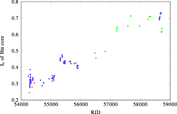
Figure 2: Top: Evolution of the central intensity of H$\alpha$ absorption core over the time interval covered by available data. Individual datasets are distinguished as follows: Red: DAO spectra; blue: Ondřejov spectra, green: amateur spectra from the BeSS database. Bottom: Time evolution of the peak intensity ($V+R$)/2 of the H$\alpha$ emission over the same interval of time.

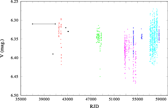
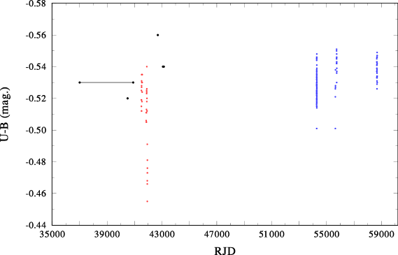
Figure 3: Top: Variation of the $V$ magnitude over the time interval covered by available data. Bottom: Variation of the $U\!-\!B$ colour over the same time interval. In both panels, data from individual observing stations listed in Table 2 are shown by coloured circles as follows: 01: blue; 10, 42, 112, and 113 (with uncertain dates of observations): black; 13: red; 61: green, 93: magenta, 114: cyan.

The long-term variations in brightness and colour (Fig. 3) are not very pronounced. We suspect some brightness decrease in the interval RJD $\sim 53000-55000$, when the H$\alpha$ emission was present in the spectra. If real, this would indicate an inverse correlation between the brightness and emission-line strength as defined by Harmanec (1983). This type of correlation is observed for objects seen more or less equator-on. The increase of the emission strength is accompanied by a light decrease. In the $U\!-\!B$ versus $B\!-\!V$ diagram, the object moves along the main sequence towards a later spectral subclass.

On the other hand, the colour–colour variations shown in Fig. 4 seem to indicate a positive correlation for stars observed more pole-on, during which the emission-strength increase is accompanied by a light brightening and a shift of dereddened colours from the main sequence to giants or supergiants of the same spectral class. This simple geometrical interpretation was confirmed by the models published by Sigut & Patel (2013).

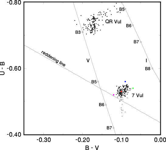
Figure 4: Variation of 7 Vul in the $U\!-\!B$ vs. $B\!-\!V$ diagram. Also shown for comparison are the variations of another Be star observed at Hvar: QR Vul. Data from individual observing stations listed in Table 2 are shown by coloured circles as follows: 01: black; 10: red; 13: open black circles; 42: magenta; 112: blue; 113: green. We note that the peculiar behavior of observations from station 13 might be due to variability of the comparison star V395 Vul, and not variability of 7 Vul itself.

4 Orbital variations

4.1 An improved ephemeris

Given the presence of secular spectral variations described in the previous section, it is not easy to apply some of the more sophisticated methods of RV measurement. This is why we opted for classical RV measurements using reSPEFO. It is also important to mention that the vast majority of our data cover only the red part of the spectrum. OND and DAO spectra contain only four stronger lines: H$\alpha$, Si ii 6347 and 6371 Å, and He i 6678 Å. The majority of the BeSS spectra cover only the H$\alpha$ region; some also cover He i 6678 Å. Only five BeSS spectra are echelle spectra, covering also blue parts of the spectrum. Since the RV zero-point can only be under control in the red region containing telluric lines, we preferred not to use RVs from the blue spectra. We are thus left with H$\alpha$, the only strong line available. For the spectra from epochs when the circumstellar matter was present, we were able to measure a sharp absorption core of H$\alpha$, while for the epochs without perceptible circumstellar matter, we could only measure the lower parts of the broader H$\alpha$ absorption profile, with a lower accuracy than that from the sharp cores. These RVs are listed in Table 9 in Appendix B.

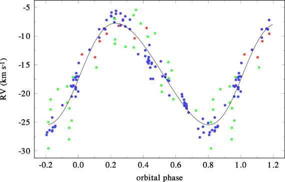
Figure 5: Top: RV curve based on all 124 RVs of the H$\alpha$ absorption and old DAO mean RVs (Plaskett & Pearce, 1931). We highlight the old DAO RVs (red; decreased in RV for the difference between the systemic velocities of these, and new spectra), new DAO and Ondřejov RVs based on a sharp line core from epochs where significant circumstellar matter is present (blue), and Ondřejov and BeSS spectra, based on RVs of broad H$\alpha$ profiles without perceptible emission (green). Our solution of Table 3 is shown by a solid line. Bottom: Phase-locked variations of the $V/R$ ratio of the double-peaked H$\alpha$ emission. For both plots, ephemeris (1) was used.

In addition to our RVs, we also used seven old DAO RVs secured between 1919 and 1925 and published as mean values of 5 to 12 lines (Plaskett & Pearce, 1931). In cases where some of the plates were measured several times, we adopted the mean RV of these measurements. For convenience, we provide these RVs together with their RJDs in Table 10 of Appendix B. Plaskett & Pearce (1931) concluded that the star has a constant velocity but we verified that all their spectra were obtained in phases close to the RV maximum of the 69.4 d orbit. Using all H$\alpha$ absorption RVs and the old mean DAO RVs (Plaskett & Pearce, 1931), we calculated several trial orbital solutions. To this aim, we used the program FOTEL (Hadrava, 2004a). Our new orbital elements are compared to those by Vennes et al. (2011) in Table 3 and the corresponding phase plot is in Fig. 5. Our solution defines a new linear ephemeris

$$T_{\rm periastr.passage}={\rm RJD\,}55986.8+69\aas@@fstack{d}4212\times E,$$ (1)

to be used throughout this paper.

Table 3: The orbital solutions for the primary component of 7 Vul.

Element	Vennes et al. (2011)	This paper
$P$ (d)	69.30$\pm$0.07	69.4212$\pm$0.0034
$T_{\rm periastr.}$	54248.1$\pm$2.7	55986.8$\pm$2.9
$T_{\rm super.c.}$	54219.4	55953.5
$e$	0.161$\pm$0.035	0.113$\pm$0.032
$\omega$ (∘)	247$\pm$16	264$\pm$16
$K_{1}$ (km s-1)	8.9$\pm$0.4	8.86$\pm$0.62
$\gamma_{1}$ (km s-1)	–	$-$49.31$\pm$0.89
$\gamma_{2}$ (km s-1)	$-$14.8$\pm$0.2	$-$16.51$\pm$0.15
$\gamma_{3}$ (km s-1)	–	$-$16.24$\pm$0.64
rms (km s-1)	not given	2.13
No. of RVs	34	123

We note that the rms errors of individual data sets are 2.17 km s^-1 for the old DAO RVs, 1.40 km s^-1 for the RVs of sharp-lined profiles, and 3.44 km s^-1 for the RVs from broad H$\alpha$ profiles. It is very encouraging that in spite of somewhat larger scatter, the RVs from more or less photospheric profiles follow the same orbit and have the same systemic velocity within the error limits. This is strong evidence that the periodic changes are indeed caused by the orbital motion. However, a word of warning is appropriate here. Sterne (1941) and Harmanec (2003) pointed out that a disturbance of line profiles that is symmetric with respect to line joining the components can lead to spurious eccentricities with $\omega$ of either $90^{\circ}$ or $270^{\circ}$. This could be the case for 7 Vul. We note that the orbital elements of 7 Vul are quite similar to those of another Be star, V744 Her = 88 Her (Harmanec et al., 1974; Doazan et al., 1982a). An eccentric orbit with $\omega\sim 270^{\circ}$ was also found. A spurious eccentricity was detected for V832 Cyg = 59 Cyg (Harmanec et al., 2002). Another good example is the Be binary BR CMi (Harmanec et al., 2015), which is also an ellipsoidal variable. A formal solution of its RV curve leads to an eccentric orbit with $\omega\sim 90^{\circ}$ but the light curve confirms a circular orbit. Therefore, the possibility that the true orbit of 7 Vul is essentially circular should be kept in mind. Another fact worth mentioning is that the old DAO RVs are systematically much more negative that the present-day RVs. Long-term RV changes with amplitudes larger than the amplitudes due to orbital motion are known for a number of Be stars, such as for example $\zeta$ Tau (Delplace, 1970) or $\gamma$ Cas (Harmanec et al., 2000). This could also be the case for 7 Vul. Regrettably, no H$\alpha$ profiles from the times of old DAO observations are available. We also mention that in some dynamical phases of the envelope evolution, the RVs of shell lines can exhibit positive or negative RV shifts with respect to their orbital RV, which could also distort the orbital RV curve based on RVs from the shell lines.

For spectra with the presence of double H$\alpha$ emission, we also derived the $V/R$ ratio of the emission peaks. As is seen in the bottom panel of Fig. 5, the $V/R$ changes also vary with the orbital period and in phase with the RV changes. This can easily be understood by the fact that the ‘nose’ of the Roche lobe around the primary is filled by a larger amount of emitting circumstellar material. Relatively large scatter of the data around a mean trend is clearly due to the fact that the emission was relatively weak throughout its presence. Phase-locked $V/R$ changes constitute another proof of the binary nature of 7 Vul. Similar variations were also found for V744 Her (Doazan et al., 1982b), V839 Her = 4 Her (Harmanec et al., 1976) and later for a number of other binary Be stars (cf., e.g. Rivinius et al., 2013).

Figure 6: Comparison of the OND spectra from different orbital cycles in the vicinity of the He i 6678 Å line. Top panel: Spectra from the elongation with the maximum RV of the primary. Bottom panel: Two spectra from the other elongation with minimum RV of the primary. The line asymmetry can clearly be seen to vary with orbital phase.

4.2 The nature of the line-profile changes of the He i 6678 Å line

Vennes et al. (2011), using phase-averaged spectra, argued that the asymmetry of the He i 6678 Å line profiles varies with the orbital phase and tentatively suggested that it might be due to the presence of a weak line of the secondary component. On the other hand - since the pioneering work by Walker et al. (1979) - it is well known that the hot emission-line stars are often exhibiting rapid line-profile changes, sometimes in the form of subfeatures travelling across the line profiles.

To get some idea of which interpretation is the most probable, we inspected the homogeneous series of the OND spectra. First, we inspected the two series of spectra taken on RJDs 54296 and 54297, of 0.18 and 0.21 d duration, respectively. We found no detectable systematic change in these profiles. On the other hand, the line profiles from different orbital cycles and from the two opposite elongations clearly demonstrate that the line asymmetry indeed varies with the orbital phase; see Fig. 6. This seems to support the conclusion by Vennes et al. (2011).

4.3 KOREL disentangling

Figure 7: Result of KOREL disentangling for 14 OND spectra secured in 2019, when the emission was almost absent. The top panel, shifted for 0.3 in normalised flux for clarity, shows the disentangled spectrum of the primary, while the bottom panel shows the disentangled spectrum of telluric lines.

Considering the above finding, it was deemed useful to carry out an attempt for spectra disentangling. We used the program KOREL (Hadrava, 2004b) for this purpose. However, with the spectra at hand, spectra disentangling is a difficult task. The strongest line at our disposal, H$\alpha$, is not usable because of its secular variations. There are only 15 OND spectra from the year 2019, when the emission was almost absent, all of which contain strong water vapour lines and are simply not numerous enough to detect a weak signal from the secondary. We are thus left with 107 line profiles of the (relatively weak) He i 6678 Å line. We first disentangled the region 6510 - 6539 Å, which contains strong water vapour lines, to derive the relative line strengths of the telluric lines for all spectra (Hadrava, 1997). These line strengths were then kept fixed in all consecutive trials.

We then disentangled the whole red spectrum of the primary (6330 - 6720 Å) from the epoch without emission. This is shown together with the disentangled telluric spectrum in Fig. 7. Lines of Si ii at 6347 and 6371 Å, Ne i 6402 Å, H$\alpha$, and He i 6678 Å are seen there. This disentangled spectrum of the primary was later used to estimate its radiative properties; see Sect. 6.1.

Table 4: An unconstrained orbital solution for the He i 6678 Å line derived by KOREL.

Element	Value
$P$ (d)	69.4212 fixed
$T_{\rm periastr.}$	55986.733
$e$	0.1077
$\omega$ (∘)	265.1
$K_{1}$ (km s-1)	8.753
$K_{2}$ (km s-1)	86.092
$m_{1}\sin^{3}i$ ($\mathcal{M}^{\mathrm{N}}_{\odot}$)	5.474
$m_{2}\sin^{3}i$ ($\mathcal{M}^{\mathrm{N}}_{\odot}$)	0.557
$\Sigma(O-C)^{2}$	19473.4
No. of RVs	102

For the final attempt, we used only the spectral region from 6665 to 6690 Å, which contains the He i 6678 Å line. Noting generally higher noise levels in the BeSS spectra in this region, we restricted our analysis to 102 DAO and OND spectra and tried to disentangle the primary and secondary line profiles, keeping all orbital elements fixed at values from Table 3. We derived the goodness-of-fit for a range of fixed values of the mass ratio as shown in Fig. 8. It is seen that there is a clearly defined minimum of the sum of squares of residuals for the mass ratios between about 0.10 and 0.15. We therefore allowed for unconstrained solutions, keeping only the orbital period fixed and seeking the solution with the lowest sum of squares of residuals. This is presented in Table 4. Disentangled line profiles of the primary and secondary, normalised to the joint continuum of the binary, are shown in Fig. 9. Measured RVs of both profiles are close to the systemic velocity of the binary of about $-16$ km s^-1, which verifies that the line in the secondary spectrum is the He i 6678 Å line and not some other line. We very roughly estimate its projected rotational velocity $v_{2}\sin i\sim 100$ km s^-1. As pointed out to us by an anonymous referee, Chojnowski et al. (2018) reported a discovery of a hot subdwarf secondary in the binary system HD 55606 with a Be primary and with orbital elements quite similar to 7 Vul: period 93$\aas@@fstack{d}$76, semi-amplitudes of 11 and 78 km s^-1 , and a mass ratio of 0.14. This leads us to a tentative conclusion that the secondary of 7 Vul is also a hot subdwarf. New high-$S/N$ echelle spectra, covering long wavelength intervals will be needed to reliably disentangle more spectral lines of the secondary and for the determination of its radiative properties. Because of the relatively cooler temperature ($T_{\rm eff}$$\sim$15000 – 16000 K) of the Be star in 7 Vul , a hot subdwarf may be easier to detect in the 7 Vul system given the lower contrast ratio compared to some other Be + hot subdwarf binaries, such as HD 55606 (Be star $T_{\rm eff}$$\sim$21000 K) and $\varphi$ Per (Be star $T_{\rm eff}$$\sim$25500 K; Frémat et al., 2005).

Figure 8: Dependence of the sum of squares of residuals on the binary mass ratio $q$ derived from the KOREL solutions in the neighbourhood of the He i 6678 Å line. All elements from our solution were kept fixed and different fixed values of the mass ratio were used. The dependence is flat but a clear minimum for mass ratios between 0.10 and 0.15 is seen.

Figure 9: Result of KOREL disentangling of both binary components in the neighbourhood of He i 6678 Å for all DAO and OND spectra. For clarity, the disentangled profile of the secondary was shifted up by 0.01. Both spectra were normalised relative to the joint continuum of the binary.

Figure 10: Combined Hvar $V$ photometry, and Hipparcos, KELT, and TESS photometries transformed to $V$ vs. phase of the 69$\aas@@fstack{d}$4212 orbital period, with phase zero corresponding to a conjunction with the Be star behind the secondary according to our orbital solution. This different phase origin is used for convenience because a possible primary eclipse should be observed near phase zero in case of a detached late-type secondary, or near phase 0.5 if the secondary is a compact subdwarf hotter than the Be primary.

4.4 Orbital light changes?

We also investigated possible orbital light variations of 7 Vul. To this purpose, we used only four sets of well-calibrated observations: Hvar $V$ magnitude, Hipparcos $H_{\rm p}$ magnitude transformed to $V$, shifted KELT $R$ magnitude, and shifted TESS magnitude. We derived robust mean values for the combined Hvar and Hipparcos transformed $V$ magnitude, and for the KELT $R$ magnitude and detrended TESS magnitudes, finding that it is necessary to subtract 0${}^{\rm m}\!\!.$8563 from the KELT data, and add 6${}^{\rm m}\!\!.$3465 to the TESS data to bring them on the scale of the $V$ magnitude. This procedure seems justified if one notes that the $V-R$ index of 7 Vul is close to zero. The corresponding phase plot is in Fig. 10. We note that there are some transient light decreases, which are systematic during the corresponding nights of observations, but these show no clear relation to orbital phases. The fact that they were occasionally detected in three considered independent photometries and also in the DAO photometry confirms their reality. For the moment, we have no clear physical interpretation for them and we were unable to confirm any periodicity in their occurrence. They are obviously quite rare. We conclude that it is possible to exclude any detectable binary eclipses in the 7 Vul system.

5 Rapid light changes

Two reports of a rapid light variability of 7 Vul were published. Koen & Eyer (2002) reported a sinusoidal variation with a period of 0$\aas@@fstack{d}$5592278 and an amplitude of 0${}^{\rm m}\!\!.$0088 from their analysis of $H_{\rm p}$ photometry. Labadie-Bartz et al. (2017) reported a period of 4$\aas@@fstack{d}$66436 from the analysis of numerous KELT photometric observations.

Omitting the DAO data, which were obtained relative to another Be variable, V395 Vul = 12 Vul, we analysed as before the combined set of the transformed Hipparcos $H_{\rm p}$ photometry, the Hvar $V$ magnitude observations, KELT $R$ photometry decreased arithmetically by 0${}^{\rm m}\!\!.$8563, and TESS detrended photometry increased by 6${}^{\rm m}\!\!.$3465 to shift them to the range of the $V$ magnitude. For the search for rapid variability, we omitted all observations fainter than 6${}^{\rm m}\!\!.$37 to exclude the non-periodic occasional light decreases mentioned above. A period search in this combined data set returned a period of 0$\aas@@fstack{d}$55917. We carried out a sinusoidal fit to obtain the most accurate value for this period, 0$\aas@@fstack{d}$55916706$\pm$0${}^{\rm m}\!\!.$00000083. The full amplitude of this variability is 0${}^{\rm m}\!\!.$00476$\pm$0${}^{\rm m}\!\!.$00013. However, since different filters are used in the various photometric datasets, and especially since the amplitude is clearly variable (as seen in the TESS data in Fig. 11), this amplitude is necessarily approximate. The corresponding sinusoidal 0$\aas@@fstack{d}$559 light curve is shown in Fig. 12. Its scatter is higher than observational errors and we attribute this to the above mentioned variations in the light-curve amplitude and to probable secular changes in the accurate value of the 0$\aas@@fstack{d}$559 period itself. The signal of the rapid light variability is clearly more complex than a simple sinusoid at a single frequency, as evidenced by the apparent amplitude variation in the TESS light curve, and the presence of many harmonics in the Fourier transform of the TESS data. A more detailed investigation of the nature of rapid variations of 7 Vul is beyond the scope of this paper and will be published elsewhere. We note that the mean 0$\aas@@fstack{d}$559 period could be interpreted as the rotational period of the primary, which we estimate in the following section to be about 0$\aas@@fstack{d}$5.

We would also like to mention that no convincing light curve could be found in the combined photometry for periods near 4$\aas@@fstack{d}$664, which was advocated by Labadie-Bartz et al. (2017). A re-analysis of the KELT photometry convincingly demonstrates that the strongest signal is at 0$\aas@@fstack{d}$559, and that the 4$\aas@@fstack{d}$664 period is an alias of the fast period with the daily sampling, i.e., frequency (4.664)${}^{-1}\sim$ 2 cycles d^-1 - (0.5592)^-1.

Figure 11: Time plot of accurate TESS photometry of 7 Vul. It is seen that the amplitude of the 0$\aas@@fstack{d}$559 period varies with time.

Figure 12: Periodic rapid light variations based on calibrated Hvar $V$ photometry, $H_{\rm p}$ photometry transformed to $V$ magnitude, KELT $R$ photometry decreased by 0${}^{\rm m}\!\!.$8563, and detrended TESS broadband magnitudes increased by 6${}^{\rm m}\!\!.$3465 to shift them to the range of $V$ photometry. All observations from rapid light decreases that were fainter than 6${}^{\rm m}\!\!.$37 were omitted. All data are plotted with the ephemeris derived from a sinusoidal fit $T_{\rm min.V}={\rm RJD}\leavevmode\nobreak\ 53000.2951(48)+0\aas@@fstack{d}55916706(83)\cdot E$. The fitted sinusoid with a semi-amplitude of 0${}^{\rm m}\!\!.$00476(13) is shown as a solid line.

6 Probable binary properties

Since we still consider the detection of the He i 6678 Å line of the secondary as tentative, we investigate the probable range of the basic physical properties along two lines using the observed and deduced properties of the primary only, and using the estimates of binary masses from the KOREL solution.

6.1 Radiative properties of the primary

Vennes et al. (2011) estimated the radiative properties of the primary of 7 Vul in several ways. Using the spectral energy distribution (SED) from the UV to IR wavelengths, these latter authors obtained $T_{\rm eff}$ = $14400\pm 800$ K and $E(\hbox{$B\!-\!V$})=0$${}^{\rm m}\!\!.$069$\pm$0${}^{\rm m}\!\!.$030. We note that for that particular study, the authors collected photometry from various sources and from different epochs. They also considered both determinations of the Hipparcos parallax $p=0\aas@@fstack{\prime\prime}00429\pm 0\aas@@fstack{\prime\prime}00076$ (Perryman & ESA, 1997), and $p=0\aas@@fstack{\prime\prime}00281\pm 0\aas@@fstack{\prime\prime}00048$ (van Leeuwen, 2007b, a). Fitting the high-dispersion Balmer-line profiles with the B-star model grid (Lanz & Hubeny, 2007), they arrived at $T_{\rm eff}$ = $15600\pm 200$ K, and log $g$ = $3.75\pm 0.02$ [cgs], and proposed the spectral class B4-5III-IVe.

To determine the radiative properties of the primary, we used the Python program PYTERPOL (Nemravová et al., 2016), which interpolates in a pre-calculated grid of synthetic spectra. Using a set of observed spectra, PYTERPOL tries to find the optimal fit between the observed and interpolated model spectra and returns the best-fit values of $T_{\rm eff}$, $v$ sin $i,$ and log $g$ .

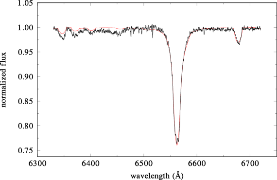
Figure 13: Comparison of the disentangled red spectrum of the primary with an interpolated synthetic spectrum for $T_{\rm eff}$ = 14910 K, log $g$ = 3.55, and $v$ sin $i,$ = 376 km s^-1. The residuals in the sense observed minus synthetic spectra are also shown in the bottom panel.

Table 5: Two distinct determinations of the radiative properties of the primary with PYTERPOL and MCMC analysis.

Element	Pollux ATLAS12 models	B-star grid
$T_{\rm eff}$ (K)	14910	15750
log $g$ [cgs]	3.55	3.61
$v$ sin $i,$ (km s-1)	376	369

In our particular application, two different grids of spectra were used: a B-star grid of line-blanketed NLTE models (Lanz & Hubeny, 2007), and the Pollux database (Palacios et al., 2010): the program fitted the disentangled spectrum of the primary from 2019 spectra (without the trace of emission) over the whole wavelength range from 6330 to 6720 Å. We then ran a Markov chain Monte Carlo (MCMC) simulation using emcee Python library by Foreman-Mackey et al. (2013). We ran 450 iterations and to our surprise, this revealed two distinct, parallel solutions. These are given in Table 5 and the fit for the cooler $T_{\rm eff}$, found originally from PYTERPOL solution, is shown in Fig. 13. It was pointed to us by our colleague M. Brož that the two separate solutions are indicative of mutual differences between the B-star and Pollux grid. The lowest $T_{\rm eff}$ of the B-star grid is 15000 K. Therefore, the two distinct solutions correspond to the two sets of synthetic spectra. Considering that the rapid stellar rotation of the primary can also affect the observed spectrum, we do not think that any more sophisticated techniques would provide us with real error estimates of the radiative properties of the primary. These are hidden in systematic differences in the different model spectra and their uncertainties. We therefore think that the difference between the two solutions represents a good guess of what the real uncertainties could be. We note that an estimate of $T_{\rm eff}$ by Vennes et al. (2011) based on the SED also falls within this range.

6.2 Luminosity, mass, and radius of the primary

Figure 14: Comparison of the range of possible values of the radius of the primary, which we estimated for the two distinct values of $T_{\rm eff}$, the range of dereddened $V$ magnitude, and the Gaia parallax. We note that the two evolutionary tracks are labelled by stellar mass.

A standard dereddening of the mean calibrated $U\!B{}V$ magnitudes from more recent Hvar observations,

$V=6$${}^{\rm m}\!\!.$337, $B\!-\!V$=$-0$${}^{\rm m}\!\!.$093, and $U\!-\!B$=$-0$${}^{\rm m}\!\!.$539,

gives

$V_{0}=6$${}^{\rm m}\!\!.$133-6${}^{\rm m}\!\!.$153, ($B\!-\!V$)${}_{0}=-0$${}^{\rm m}\!\!.$157, ($U\!-\!B$)${}_{0}=-0$${}^{\rm m}\!\!.$585, with E($B\!-\!V$)=0${}^{\rm m}\!\!.$064. The range in the magnitude corresponds to the adopted range of $A_{\rm V}$ from 2${}^{\rm m}\!\!.$9 to 3${}^{\rm m}\!\!.$2.

Using the accurate Gaia Data Release 2 parallax (Gaia Collaboration et al., 2016, 2018),

$p=0\aas@@fstack{\prime\prime}003473\pm 0\aas@@fstack{\prime\prime}000048,$

the range of $V_{0}$ and both possible values of $T_{\rm eff}$, we obtain the primary radius $R$ = 3.75 - 4.02 $\mathcal{R}^{\mathrm{N}}_{\odot}$, which is notably smaller than that estimated by Vennes et al. (2011). The corresponding range of the absolute magnitude $M_{\rm bol}$ is from $-2$${}^{\rm m}\!\!.$35 to $-2$${}^{\rm m}\!\!.$52.

In Fig. 14 we compare our radii with the evolutionary tracks of Schaller et al. (1992) in the $\log\leavevmode\nobreak\ R$ versus $\log\leavevmode\nobreak\ T_{\rm eff.}$ diagram. From this comparison, we calculate the probable mass of the primary to be $m_{1}=4.8\pm 0.1$ $\mathcal{M}^{\mathrm{N}}_{\odot}$, which is quite plausible for a B4-5IV star.

In passing we note that our values of the mass and radius would imply log $g$  $\sim 3.9$ [cgs]. This is higher than the values of $\sim 3.6$ or $\sim 3.75$ [cgs] estimated by Vennes et al. (2011). Since the Balmer-line profiles are the most sensitive to log $g$, we propose that they have been affected by some amount of emission from circumstellar matter throughout the whole documented spectral history of the star.

Table 6: Probable mass ratio $q=m_{2}/m_{1}$ and the mass of the secondary estimated for several orbital inclinations $i$, $m_{1}=4.8$ $\mathcal{M}^{\mathrm{N}}_{\odot}$ , and our orbital solution.

$i$	$m_{2}$	$q$
(degs.)	($\mathcal{M}^{\mathrm{N}}_{\odot}$)
90.0	0.5180	0.1079
80.0	0.5266	0.1097
70.0	0.5538	0.1154
60.0	0.6047	0.1260
50.0	0.6908	0.1439
40.0	0.8379	0.1746
30.0	1.1118	0.2316

6.3 Probable physical properties of the binary system

Table 7: Masses of the binary components estimated for several possible orbital inclinations from the KOREL solution of Table 4.

$i$	$m_{1}$	$m_{2}$
(degs.)	($\mathcal{M}^{\mathrm{N}}_{\odot}$)	($\mathcal{M}^{\mathrm{N}}_{\odot}$)
90.0	5.47	0.56
80.0	5.73	0.58
70.0	6.60	0.67
58.0	8.98	0.91

If we adopt the mass of 4.8 $\mathcal{M}^{\mathrm{N}}_{\odot}$ and our orbital solution, we can estimate the mass ratio and the mass of the secondary for a few different orbital inclinations. These are summarised in Table 6. If we assume that the axis of orbital revolution and the axis of the rotation of the primary are parallel, we can set a lower limit for the orbital inclination. Adopting the Roche model approximation, we have $R_{\rm equator}=1.5R_{\rm pole}$. In the limiting case of break-up rotation of the primary, we can roughly approximate the area, from which we receive the stellar flux of the primary (estimated from dereddened observed $V$ and parallax) by an effective radius $R_{ef}$, for which we have (assuming the area of an ellipse),

$$\pi R_{\rm pole}R_{\rm equator}=\pi R^{2}_{ef}\rightarrow R_{\rm equator}=\sqrt{3/2}R_{ef}.$$ (2)

For $R_{ef}\approx 3.9$ $\mathcal{R}^{\mathrm{N}}_{\odot}$, $R_{\rm equator}\approx 4.8$ $\mathcal{R}^{\mathrm{N}}_{\odot}$. Consequently, for critical rotation at the equator, we obtain $\approx 440$ km s^-1, which implies that the inclination must be higher then about $58^{\circ}$. It is notable that this last estimate agrees well with that of Vennes et al. (2011), although we used different values of basic physical properties of the system. Finally, we note that the probable rotational period of the primary should be between about 0$\aas@@fstack{d}$45 and 0$\aas@@fstack{d}$53 for the range of inclinations from $58^{\circ}$ to $90^{\circ}$.

Using a different approach, Kervella et al. (2019) estimated the mass and radius of the 7 Vul primary as

$m=5.00\pm 0.25$ M_⊙  and $R=4.64\pm 0.23$ R_⊙.

If we assume that the 0$\aas@@fstack{d}$5592 period is the rotational period of the primary and adopt our $v$ sin $i,$ = 370 km s^-1, we find $R_{\rm equator}=4.09-4.82$ $\mathcal{R}^{\mathrm{N}}_{\odot}$ for the same range of inclinations as above.

Finally, if we use the KOREL solution shown in Table 4, we obtain possible masses of both components as a function of orbital inclination. These are listed for several plausible values of the inclination in Table 7. From this, we conclude that the true orbital inclination should be higher than some $70^{\circ}$.

7 Conclusions

Our analysis confirms the binary nature of 7 Vul and a low mass for its companion. We underline that our estimates are preliminary due to all the problems we have discussed above. The secondary cannot be a cool Roche-lobe-filling object because, were this the case, its spectral lines would have been detected in the observed spectra (cf, e.g. Harmanec et al., 2015). In principle, it could be a normal star of a late spectral class but the existence of such companions to Be stars has not yet been proven. It is much more probable that this secondary is a hot subdwarf like that observed by Gies et al. (1998) for $\varphi$ Per; see also the recent search for such systems in the existing IUE spectra (Wang et al., 2018) and the detection of a hot subdwarf for HD 55606 (Chojnowski et al., 2018). To the best of our knowledge, there are no high-dispersion far-UV spectra of 7 Vul. In order to make progress in the understanding of this system, we feel it necessary to first of all obtain a series of high-S/N far-UV spectra over the whole 69.4 d period and search for the possible presence of lines of a hot subdwarf secondary. We believe it would furthermore be helpful to monitor the H$\alpha$ profile of the star from time to time and to obtain another series of high-resolution high-S/N optical echelle spectra, when the star appears again as a normal rapidly rotating B star, and to carry out a much more accurate orbital analysis and line-profile modelling. Lastly, several whole-night series of high-S/N spectral observations could be used to check for the presence of mild rapid line-profile variations, possibly related to the rapid periodic light changes.

Appendix A Details on the photometric data reductions and homogenisation

Table 8: Accurate Hvar all-sky mean $U\!B{}V$ values for all comparison stars used. These were added to the magnitude differences var.$-$comp. and check$-$comp. for data from all stations.

Star	HD	No. of	$V$	$B$	$U$	$(B-V)$	$(U-B)$
		obs.	(mag.)	(mag.)	(mag.)	(mag.)	(mag.)
5 Vul	182919	3	5.65$\pm$0.010	5.66$\pm$0.011	5.62$\pm$0.012	0.01	-0.04
9 Vul	184606	30	5.010$\pm$0.009	4.906$\pm$0.011	4.499$\pm$0.012	-0.104	-0.407
V395 Vul	187811	24	4.928$\pm$0.015	4.759$\pm$0.017	4.104$\pm$0.020	-0.170	-0.654
13 Vul	188260	38	4.584$\pm$0.008	4.536$\pm$0.010	4.404$\pm$0.012	-0.048	-0.132

Since we used photometry from several sources and photometric systems, both all-sky and differential, relative to several different comparison stars, we attempted to arrive at some homogenisation and standardisation. We derived improved all-sky values for all comparison stars used, employing carefully standardised $U\!B{}V$ observations secured at Hvar specifically for this purpose. The adopted values are collected in Table 8 together with the number of all-sky observations and the rms errors of one observation. These were added to the respective magnitude differences to obtain directly comparable standard $U\!B{}V$ magnitudes for all stations.

Below, we provide some details of the individual data sets and their reductions.

• Station 01 – Hvar:   These differential observations were secured by PH and HB, and the more recent ones also by students A. Oplištilová and K. Vitovský, relative to either 9 Vul or 13 Vul. They were carefully transformed to the standard $UBV$ system via non-linear transformation formulæ using the HEC22 reduction program; see Harmanec et al. (1994) and Harmanec & Horn (1998) for the observational strategy and data reduction. All observations were reduced with the latest HEC22 rel.18 program, which allows the time variation of linear extinction coefficients to be modelled in the course of observing nights. The whole archive of Hvar photometry since 1972 will be published elsewhere after a thorough revision (Božić et al.; in prep.).

• Station 10 – Kitt Peak (KPNO):    These are all-sky $U\!B{}V$ observations published only as the mean values

  $V$=6${}^{\rm m}\!\!.$31, $B\!-\!V$=$-0$${}^{\rm m}\!\!.$10, and $U\!-\!B$=$-0$${}^{\rm m}\!\!.$53

  and without times of observations. These were secured at some point between RJD 37700 and 40900. We have to accept these published values as they are because none of the comparisons observed at Hvar have been observed (the only exception being the variable V395 Vul).

• Station 13 – Mt. Kobau:   These differential observations were obtained in the DAO (33), (44), and (55) medium-band system. We transformed them into the Johnson $U\!B{}V$ system using the transformation formulæ devised by Harmanec & Božić (2001). Unfortunately, another Be star V395 Vul was used as the comparison star for these observations. However, it seems that the secular variations of V395 Vul are not large. Its photometry by Crawford et al. (1971) gives $V=4$${}^{\rm m}\!\!.$94, $B\!-\!V$$=-0$${}^{\rm m}\!\!.$16, and $U\!-\!B$$=-0$${}^{\rm m}\!\!.$66, which are values quite close to the Hvar photometry; see Table 8. Nevertheless, the Hipparcos $H_{\rm p}$ photometry shows variability of V395 Vul on about 0${}^{\rm m}\!\!.$1 level (Perryman & ESA 1997).

• Station 42 – Dyer:   These differential observations relative to 5 Vul were obtained around RJD 40500 and published as the mean values

  $V$=6${}^{\rm m}\!\!.$39, $B\!-\!V$=$-0$${}^{\rm m}\!\!.$12, and $U\!-\!B$=$-0$${}^{\rm m}\!\!.$52.

  They were corrected for extinction and transformed to the standard Johnson $U\!B{}V$ system by the original authors.

• Station 61 – Hipparcos $H_{\rm p}$:   These space observations were extracted from the ESA archive (Perryman & ESA 1997) and transformed to the standard Johnson $V$ magnitude using the transformation formula by Harmanec (1998). Only observations with error flags 0 and 1 were used.

• Station 93 – ASAS3 V photometry:   We extracted these all-sky observations from the ASAS3 public archive (Pojmanski 2002) using the data for diaphragm 1, which had on average the lowest rms errors. We omitted all observations of grade D and observations with rms errors larger than 0${}^{\rm m}\!\!.$04. We also omitted a strongly deviating observation at HJD 2452662.6863.

• Station 110 – TESS satellite   These all-sky broad-band observations are publicly available via the Mikulski Archive for Space Telescopes (MAST). The initial reductions of these were carried out by one of the present authors (J.L-B.). We note that 7 Vul was observed in TESS sector 14, and the light curve was extracted from the full-frame images at a cadence of 30 minutes using the lightkurve package.

• Station 112 – Kutztown:   These all-sky $U\!B{}V$ data are published as the mean values

  $V$=6${}^{\rm m}\!\!.$32, $B\!-\!V$=$-0$${}^{\rm m}\!\!.$09, and $U\!-\!B$=$-0$${}^{\rm m}\!\!.$56

  and were secured during 17 nights during the approximate epoch RJD 42700.

• Station 113 – Mitaka:    These 100 all-sky observations secured during 18 nights between Oct 22 and Dec 26, 1976 (RJD $\sim 43100$) are again published as the mean values only:

  $V$=6${}^{\rm m}\!\!.$33, $B\!-\!V$=$-0$${}^{\rm m}\!\!.$07, and $U\!-\!B$=$-0$${}^{\rm m}\!\!.$54.

• Station 114 – ASAS-SN V photometry:   We extracted these all-sky observations from the ASAS-SN archive. They are all from the bc camera in Hawaii and their scatter is not negligible. We removed all observations with an rms error higher than 0${}^{\rm m}\!\!.$009 and used only observations within the magnitude range from 6${}^{\rm m}\!\!.$65 to 6${}^{\rm m}\!\!.$80. Finally, comparing the robust mean value from the Hvar calibrated $V$ photometry and from the cleaned ASAS-SN observations, we derived a correction of $-0$${}^{\rm m}\!\!.$380 to bring the ASAS-SN data to the mean Hvar $V$ magnitude.

• Station 115 – KELT (Kilodegree Extremely Little Telescope) at Winer Observatory, USA; broad-band $R$ photometry: We adopted these observations from the paper of Labadie-Bartz et al. (2017) and decreased all observed values for 0${}^{\rm m}\!\!.$856 to bring them into the range of $V$ photometry for our analyses.

Appendix B Details of the spectral data reduction and measurements

The initial reduction of all OND and DAO spectra (bias subtraction, flat-fielding, creation of 1D spectra, and wavelength calibration) was carried out in IRAF. Optimal extraction was used. Normalisation and RV measurements of H$\alpha$ absorption were carried out with the program reSPEFO. The RV measurements are based on the comparison of direct and flipped line profiles in normalised spectra. Additionally, we also measured a selection of unblended water vapour lines and their robust mean RVs were used to fine corrections of the RV zero point of each spectrogram.

Table 9: Individual RVs (in km s^-1) of the H$\alpha$ absorption measured on new DAO, OND, and BeSS spectra with reSPEFO.

RJD	RV	Observatory	RJD	RV	Observatory
54276.8204	-13.17	DAO	55373.5085	-8.85	OND
54339.7281	-7.15	DAO	55377.3711	-7.60	OND
54340.7416	-6.57	DAO	55377.3836	-6.90	OND
54367.7330	-23.33	DAO	55429.3155	-18.60	OND
54443.6185	-26.81	DAO	55429.3230	-18.68	OND
54244.4463	-22.06	OND	55430.3259	-18.92	OND
54286.4843	-14.41	OND	55430.3334	-19.28	OND
54288.3624	-17.14	OND	55431.3336	-17.05	OND
54288.5549	-16.67	OND	55431.3413	-19.66	OND
54289.5548	-17.64	OND	55461.3135	-14.06	OND
54295.4775	-20.14	OND	55462.3026	-17.46	OND
54295.5953	-20.54	OND	55463.2886	-17.46	OND
54296.3730	-21.08	OND	55464.2872	-15.35	OND
54296.5439	-22.12	OND	55470.2794	-20.34	OND
54296.5632	-21.70	OND	55483.2938	-27.65	OND
54296.5809	-21.54	OND	55625.7053	-25.15	OND
54297.4056	-21.85	OND	55648.5782	-8.82	OND
54297.4426	-22.57	OND	55648.5925	-10.28	OND
54297.5462	-22.20	OND	55650.6278	-8.71	OND
54297.5813	-22.60	OND	55675.5853	-17.01	OND
54304.4063	-24.42	OND	55777.3572	-20.56	OND
54304.5040	-25.79	OND	55834.3867	-27.21	OND
54307.3585	-26.78	OND	55878.1764	-14.34	OND
54308.3633	-26.39	OND	55878.2884	-11.57	OND
54309.5100	-24.20	OND	55879.2138	-14.85	OND
54317.5246	-18.69	OND	55879.3118	-14.66	OND
54318.5311	-17.62	OND	55906.1654	-26.60	OND
54319.3650	-17.22	OND	55906.2346	-26.45	OND
54325.4170	-12.39	OND	58640.3665	-6.74	OND
54387.2461	-20.54	OND	58640.3993	-11.07	OND
54387.3810	-18.83	OND	58640.5103	-10.34	OND
54389.2323	-16.46	OND	58648.3710	-6.09	OND
54389.2493	-17.62	OND	58649.3894	-5.20	OND
54389.3731	-17.05	OND	58651.4545	-7.56	OND
54390.2819	-14.70	OND	58654.4355	-9.83	OND
54649.5466	-26.16	OND	58681.3902	-24.72	OND
54706.5216	-17.80	OND	58681.4217	-29.31	OND
54753.2694	-6.13	OND	58682.3705	-20.78	OND
54753.2881	-5.61	OND	58689.4461	-18.51	OND
54934.5948	-25.90	OND	58689.4575	-21.33	OND
55043.4394	-12.49	OND	58690.3439	-25.72	OND
55043.4541	-13.49	OND	58690.4058	-22.31	OND
55044.3682	-14.48	OND	58691.3792	-24.45	OND
55045.5963	-15.50	OND	58714.3611	-11.60	OND
55074.3366	-25.84	OND	56480.4756	-15.19	BeSS
55074.4756	-25.65	OND	56817.5138	-16.89	BeSS
55096.3567	-7.21	OND	57224.5244	-22.53	BeSS
55098.2608	-6.49	OND	57579.5281	-27.70	BeSS
55098.4263	-6.58	OND	57676.5577	-11.72	BeSS
55098.4422	-5.90	OND	58729.6276	-18.33	BeSS
55114.2697	-14.76	OND	56508.3994	-19.46	BeSS
55114.3802	-13.68	OND	58310.4416	-9.25	BeSS
55310.6018	-6.06	OND	58338.3540	-19.00	BeSS
55310.6162	-8.16	OND	58663.4813	-17.09	BeSS
55311.6199	-7.29	OND	57205.3757	-14.29	BeSS
55312.6144	-8.33	OND	57970.3965	-15.72	BeSS
55314.5922	-8.81	OND	57207.5716	-20.73	BeSS
55314.6030	-7.15	OND	58258.4909	-22.72	BeSS

Table 10: Individual RVs of the primary from old DAO spectra (Plaskett & Pearce 1931). We derived RJDs and averaged RVs in cases where the same plate was measured several times. The RVs are mean values based on measurements of 5 to 12 spectral lines of h i and He i in the blue spectral region.

RJD	mean RV	No. of	RJD	mean RV	No. of
	(km s-1)	lines		(km s-1)	lines
22185.7940	-46.5	5-7	23992.7564	-43.7	9
22249.5973	-46.0	7-10	24000.7913	-41.0	9
22537.8743	-42.4	10	24359.8474	-41.4	12
22549.7940	-43.2	8

Appendix C The Java reduction program reSPEFO

reSPEFO is a modern refresh of the original program SPEFO, a simple yet powerful program for 1D spectra analysis written in Turbo Pascal (Horn et al. 1996; Škoda 1996; Krpata 2008).

The new version of reSPEFO is written in Java using contemporary tools with an improved user interface and functionality. The program is distributed as a runnable .jar archive. It has minimal system requirements and runs on most Linux, Windows, and MacOS systems.

It consists of a suite of tools for operations with linear spectra. The current version provides these functions:

1. Creation of a list of spectra available in a given directory, which contains running numbers of the spectra in an increasing order in time, their original names, and HJDs;

2. Converting the names of all spectra into a format compatible with the DOS convention used in the original SPEFO, i.e. three characters representing the name of the set of spectra, a five-digit running number, and the extension describing the type of spectra;

3. Import of spectra recorded in the original internal format of SPEFO;

4. Interactive rectification of spectra;

5. Interactive cleaning of cosmic ray hits and other flaws;

6. Comparison of two selected spectra with a possibility to move the second spectrum in RV and proportionally reduce its flux;

7. Interactive RV measurements based on a comparison of direct and flipped line-profile images. Individual lines of groups of lines can be put into different user-defined groups;

8. Export of all RV measurements into a table containing HJDs and RVs of individual groups of lines chosen by the user (if telluric lines were also measured, a file with a fine correction of the RV zero point is also created); and

9. Export of the spectra into either FITS or ASCII format.

Screenshots illustrating some of these features are provided in Figs. 15, 16, and 17.

The application reSPEFO is available for free under the Eclipse Public License 2.0 at https://astro.troja.mff.cuni.cz/projects/respefo, where a detailed User Guide is also provided.

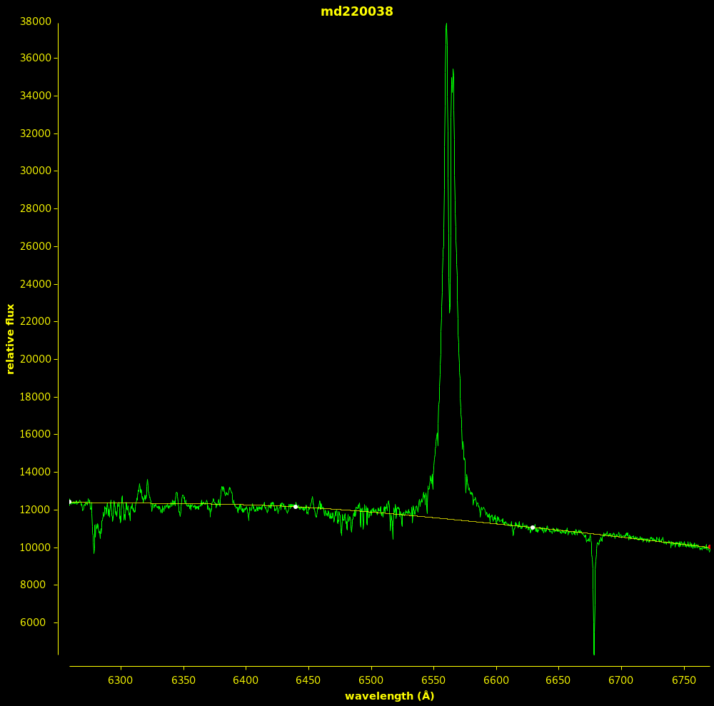
(a) Original spectrum

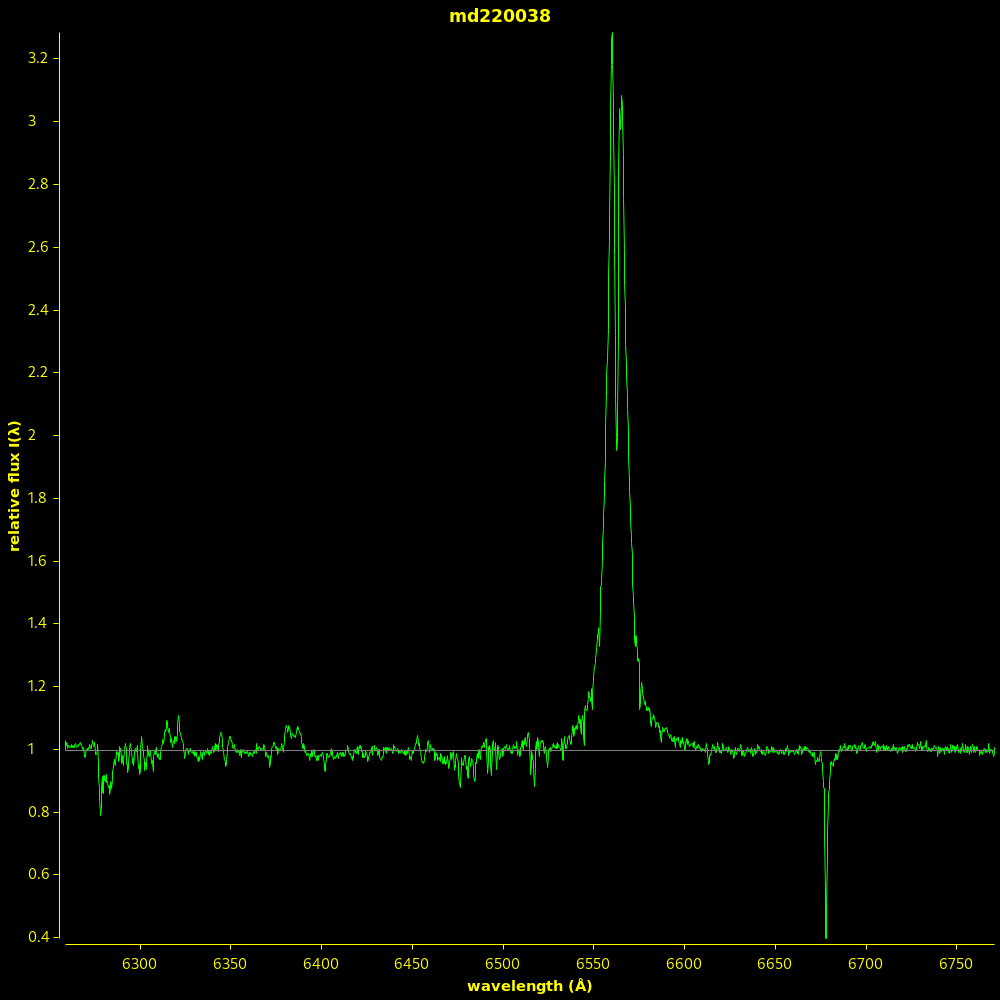
(b) normalised spectrum

Figure 15: Interactive spectra normalisation. A spectrum of V1294 Aql, a Be star with strong H$\alpha$ emission, is shown here.

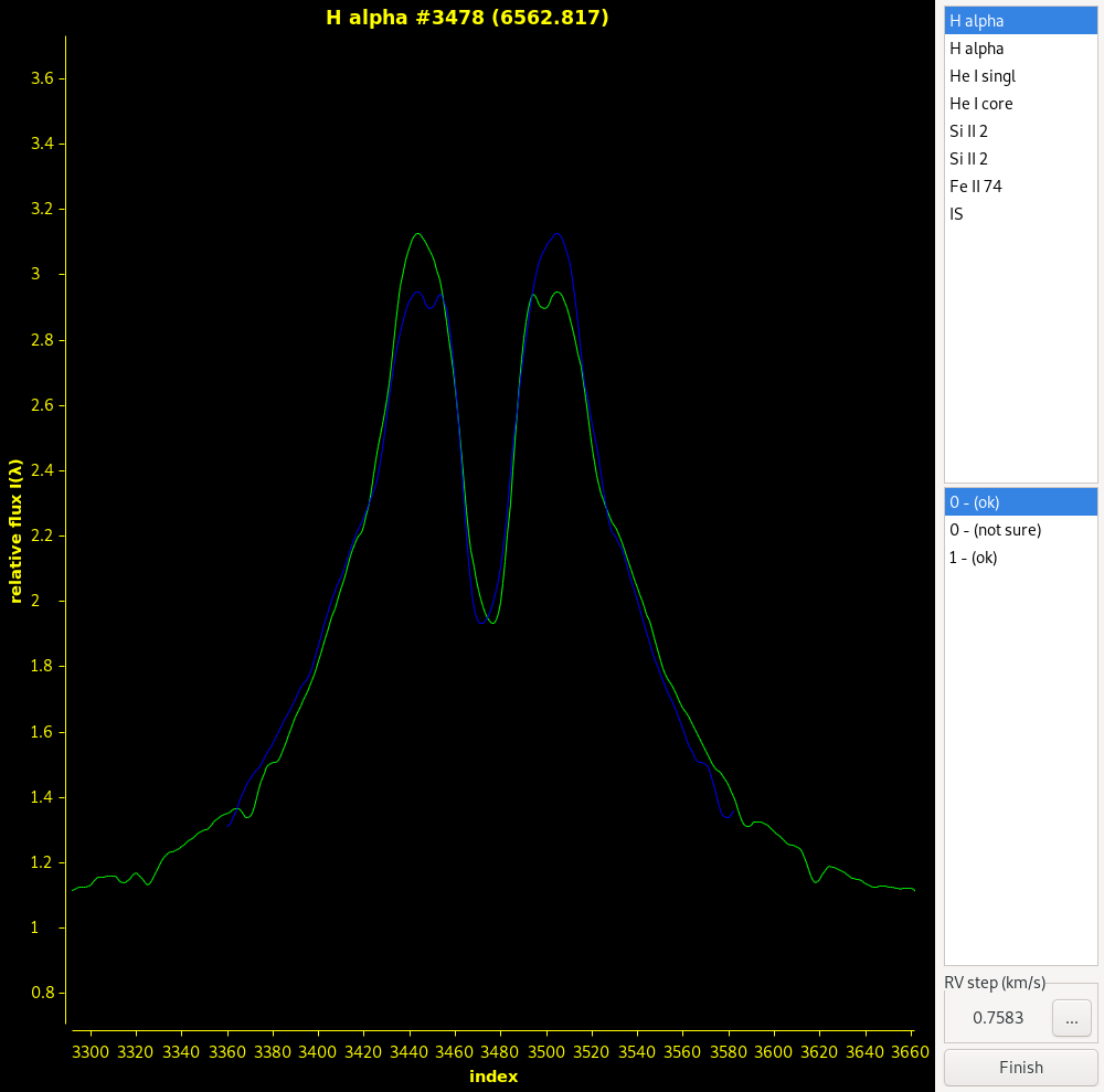
Figure 16: Interactive RV measurements: RV of the central absorption core is measured in this example. It is seen that when one would set on the outer emission-line wings, a different RV would be obtained. Measuring points are defined in a separate file using an identification and a laboratory wavelength as shown in the list in the top-right corner. The user can make multiple measurements on a single point supplemented with an optional comment as shown in the list in the bottom-right corner. Once again, a spectrum of V1294 Aql was used here.

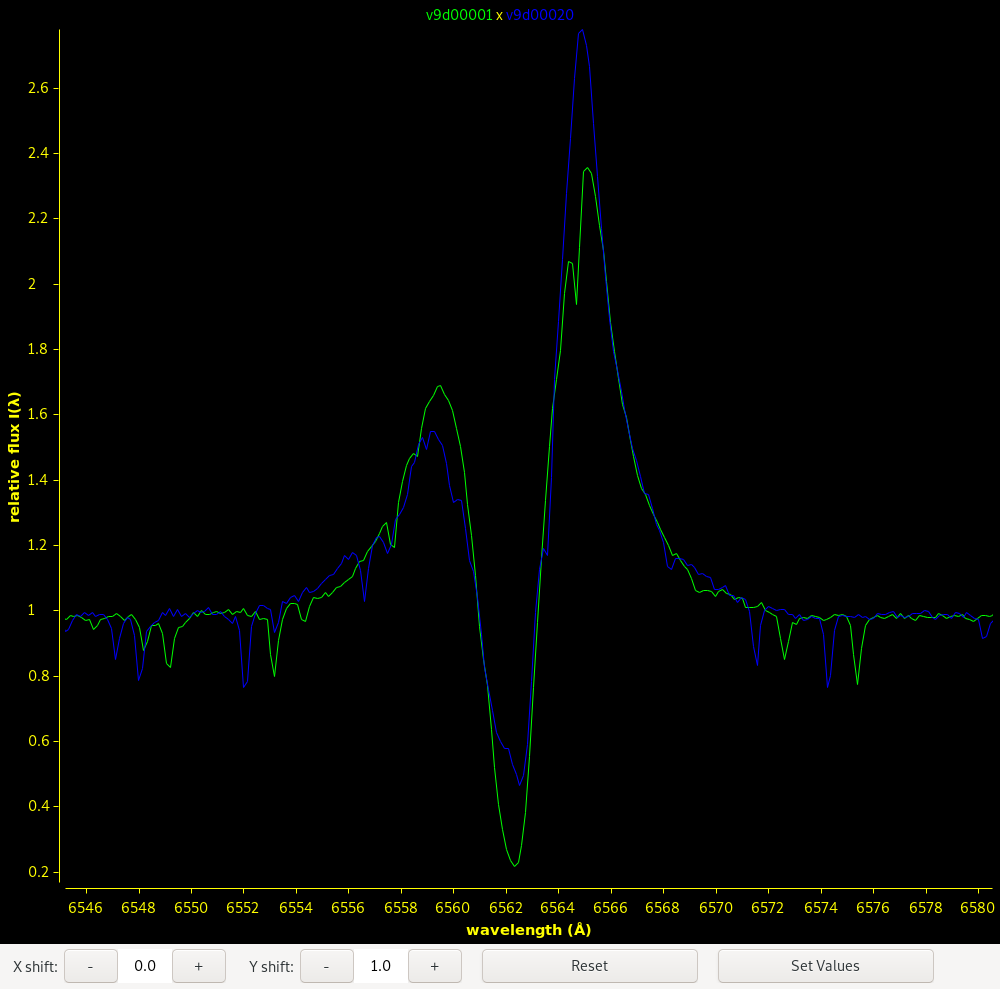
Figure 17: Comparison of two DAO spectra of 7 Vul. Mutual shifts of the profiles can be carried out interactively and the difference in RV is displayed. It is also possible to change the relative strength of the second spectrum (shown in blue).