Point2Mesh: A Self-Prior for Deformable Meshes

Abstract.

In this paper, we introduce Point2Mesh, a technique for reconstructing a surface mesh from an input point cloud. Instead of explicitly specifying a prior that encodes the expected shape properties, the prior is defined automatically using the input point cloud, which we refer to as a self-prior. The self-prior encapsulates reoccurring geometric repetitions from a single shape within the weights of a deep neural network. We optimize the network weights to deform an initial mesh to shrink-wrap a single input point cloud. This explicitly considers the entire reconstructed shape, since shared local kernels are calculated to fit the overall object. The convolutional kernels are optimized globally across the entire shape, which inherently encourages local-scale geometric self-similarity across the shape surface. We show that shrink-wrapping a point cloud with a self-prior converges to a desirable solution; compared to a prescribed smoothness prior, which often becomes trapped in undesirable local minima. While the performance of traditional reconstruction approaches degrades in non-ideal conditions that are often present in real world scanning, i.e., unoriented normals, noise and missing (low density) parts, Point2Mesh is robust to non-ideal conditions. We demonstrate the performance of Point2Mesh on a large variety of shapes with varying complexity.

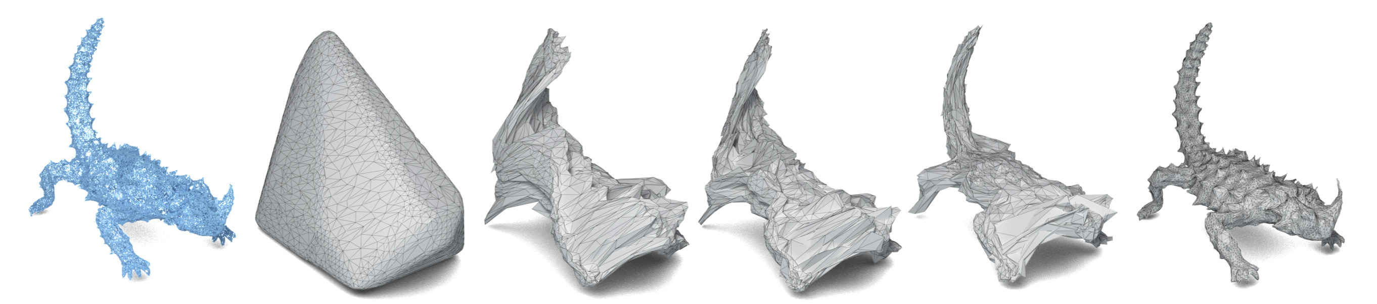
Figure 1. Starting with an input point cloud (left) and a deformable mesh, we iteratively shrink-wrap the input, leading to a watertight reconstruction.

1. Introduction

Reconstructing a mesh from a point cloud is a long-standing problem in computer graphics. In recent decades, various approaches have been developed to reconstruct shapes for an array of applications [Berger et al., 2017]. The reconstruction problem is ill-posed, making it necessary to define a prior which incorporates the expected properties of the reconstructed mesh. Traditionally, priors are manually designed to encourage general properties, like piece-wise smoothness or local uniformity.

The recent emergence of deep neural networks carries new promise to bypass manually specified priors. Studies have shown that filtering data with a collection of convolution and pooling layers results in a salient feature representation, even with randomly initialized weights [Saxe et al., 2011; Gaier and Ha, 2019]. Convolutions exploit local spatial correlations, which are shared and aggregated across the entire data; while pooling reduces the dimensionality of the learned representation. Since shapes, like natural images, are not random, they have a distinct distribution which fosters the powerful intrinsic properties of CNNs to garner self-similarities.

In this paper, we introduce Point2Mesh, a method for reconstructing meshes from point clouds, where the prior is defined automatically by a convolutional neural network (CNN). Instead of explicitly specifying a prior, it is learned automatically from a single input point cloud, without relying on any training data or pre-training, in other words, a self-prior. In contrast, supervised learning paradigms demand large amounts of input (point cloud) and ground-truth (surface) training pairs (i.e., data-driven priors), which often entails modeling the acquisition process. An appealing aspect of Point2Mesh is that it does not require knowing the distribution of noise or partiality during training, bypassing the need for large amounts of labeled training data from a particular distribution. Instead, Point2Mesh optimizes a CNN-based self-prior during inference time, which leverages the self-similarity present within a single shape.

\begin{overpic}[width=241.84842pt]{figures/06_experiments/068_self_similarity/sphere_rail-1.jpg} \put(12.0,-2.0){{\color[rgb]{0,0,0}Input}} \put(40.5,-2.0){{\color[rgb]{0,0,0}Smooth-prior}} \put(76.0,-2.0){{\color[rgb]{0,0,0}Self-prior}} \end{overpic}

Figure 2. Reconstructing a complete mesh from a point cloud with missing regions using a smooth-prior ignores the character of the global shape. The self-prior in Point2Mesh inherently learns and leverages the recurrences present within a single shape, leading to a more plausible reconstruction.

To reconstruct a mesh, we take an optimization approach, where an initial mesh is iteratively deformed to fit the input point cloud by a series of steps conducted by a CNN (Figure 1). Since objects are solid, the reconstructed model must be watertight. Therefore, we start with a watertight mesh, and deform it by displacing the vertex positions in incremental steps, to preserve the required watertight property. The initial deformable mesh can be estimated using different techniques that roughly approximate the input shape with an arbitrary genus.

Neural networks have an implicit tendency to learn regularized weights [Achille and Soatto, 2018], and converge to low-entropy solutions even for single images [Gandelsman et al., 2019]. Since Point2Mesh encodes the entire shape into the parameters of a CNN, it leverages the representational power of networks to inherently remove noise and outliers. Accordingly, this powerful self-prior excels at modeling natural shapes, whereas noisy and unnatural shapes are not well explained by the CNN (see Figure 3). A notable advantage of Point2Mesh, especially when compared to classic techniques, is its ability to cope with non-ideal conditions which are often present in real world scanning, i.e., unoriented normals, noise and / or missing regions. The classic Poisson surface reconstruction [Kazhdan et al., 2006] technique assumes oriented normals, a condition which is often hard to meet [Huang et al., 2009].

Point2Mesh optimization relies on MeshCNN [Hanocka et al., 2019], which offers the platform for a convolutional neural network applied on meshes. MeshCNN learns convolutional kernels directly on the edges of the mesh for tasks like classification and segmentation. In this work, we extend the capabilities of MeshCNN to handle shape regression. To best explain the input shape, the CNN weights must leverage the self-similarity present in natural shapes, by aggregating local attributes specific to the entire reconstructed shape. On the one hand, convolutions are applied locally to extract salient features; on the other, the same local kernels are utilized over the whole shape. Optimizing kernel weights globally across the entire shape, inherently encourages local-scale geometric self-repetition across the shape surface. Accordingly, the structure of a CNN inherently encapsulates the essence of natural shapes, which we leverage as a self-prior for reconstructing mesh surfaces.

We demonstrate the performance of Point2Mesh on variety of shapes with varying complexity, including real scans obtained from a NextEngine 3D laser scanner. We demonstrate the applicability of our approach to reconstruct a mesh from point samples containing noise, unoriented / unknown normals and / or missing regions, and compare to several other leading techniques. In particular, we demonstrate the advantage of a network over the ubiquitous smoothness prior, and pure optimization (of the same objective) with no network prior, to emphasize the strength of our self-prior.

\begin{overpic}[width=284.52756pt]{figures/03_overview/031_noise_prior_vase_landscape.jpg} \put(8.5,2.5){{\color[rgb]{0,0,0}(a)}} \put(30.0,2.5){{\color[rgb]{0,0,0}(b)}} \put(52.0,2.5){{\color[rgb]{0,0,0}(c)}} \put(85.0,2.5){{\color[rgb]{0,0,0}(d)}} \end{overpic}

Figure 3. The CNN structure inherently prefers reconstructing natural shapes. Graph of reconstruction error vs. optimization iterations (left) for reconstructing four different shapes: (a) natural shape, (b) shape + noise, (c) shuffled vertices and (d) uniform noise. The network is able to best reconstruct the natural shape (a), and struggles to reconstruct noisy and chaotic (unnatural) shapes (b,c,d).

2. Related Work

Surface Reconstruction

There has been a lot of research on the inverse problem of reconstructing a surface from a point cloud. Early works approached the reconstruction problem by fitting implicit functions to the point cloud [Hoppe et al., 1992], and then generating a mesh over its zero-set. Most previous works on surface reconstruction have focused on data consolidation [Ohtake et al., 2003; Lipman et al., 2007; Huang et al., 2009; Miao et al., 2009; Öztireli et al., 2010; Huang et al., 2013], that is, denosing, smoothing, up-sampling, or generally, enhancing the given point cloud.

The most popular method for surface reconstruction is Poisson reconstruction [Kazhdan et al., 2006; Kazhdan and Hoppe, 2013], which formalizes the problem of surface reconstruction as a Poisson system. Finding an indicator function whose gradient is the vector field characterized by the sample points and normals, enables reconstruction of the surface. Alternative approaches define the indicator function using Fourier coefficients [Kazhdan, 2005] and Wavelets [Manson et al., 2008]. Another class of approaches partitions the implicit function into multiple scales [Ohtake et al., 2003; Nagai et al., 2009]. Ohtake et al. [2005] use the compact radial basis functions (RBFs) to build the implicit surface.

Poisson reconstruction, like most previous approaches, processes point sets in local regions, in order to facilitate a post-process triangulation and mesh reconstruction. These methods do not enforce global constraints on the generated mesh, and, in particular, they require perfect normal orientation (i.e., each normal points outside of the surface) to guarantee that the reconstructed surface is watertight. Since perfect normal orientation is a cumbersome requirement, an alternative approach [Hornung and Kobbelt, 2006] relaxes this requirement by computing a dilated voxel crust and extracts the final closed surface via graph-cut minimization.

Surface reconstruction has also been approached via mesh deformation, whereby an initial mesh is iteratively deformed to fit a given point cloud [Sharf et al., 2006; Li et al., 2010]. This approach is analogous to active contours, also referred to as Snakes [Kass et al., 1988; Xu et al., 1998; McInerney and Terzopoulos, 2000]. Such optimizations are highly non-convex and often lead to local minima. To alleviate the inherent ambiguities, such techniques must define strong priors, which are explicitly hand-crafted, for example, encouraging locally uniform and piece-wise smooth reconstructions.

The most related work to Point2Mesh is the work of Sharf et al.  [2006]. Their approach reconstructs a watertight surface, via a series of iterative optimizations. Starting from an initial spherical mesh placed within the point cloud, the mesh is deformed in the direction of the face normals to fit the target point cloud. Unlike  [Sharf et al., 2006], where the mesh is inflated starting inside and moving out, we approach the mesh fitting from outside-in. To avoid local minima, Sharf et al. used smoothness priors and heuristics to split and prioritize the advancing fronts. The key meta difference of our method (beyond technical details) is that we do not design the prior; instead, we learn the prior from the input shape itself.

Neural Self-Priors

The inspiration for Point2Mesh comes from 2D image processing, in particular the work of Ulyanov et al.  [2018] and other works that focus on self-similarity within images, e.g., [Shocher et al., 2018; Gandelsman et al., 2019; Zhou et al., 2018; Shaham et al., 2019; Sun et al., 2019]. The concept of Deep Image Prior (DIP) [Ulyanov et al., 2018] is intriguing, yet, still not fully understood. In our work, we not only use a similar concept for surface reconstruction, but show empirically that the weight-sharing of the CNN network is a key element in the advantage of self priors. We believe that this directs the network to learn (non-local) repeating structures within the processed data (mesh, in our case). The notion of exploiting symmetry and repetitions in 3D shapes has been explored in classic shape analysis techniques [Nan et al., 2010; Pauly et al., 2008]. Harary et al. [2014] demonstrated surface holes can be completed using patches from within the same object.

Geometric Deep Learning and Reconstruction

Recently, the concept of a differential 3D rendering as a plug-and-play component in a computer graphics pipeline has gained increasing interest. An application of a differential rendering module is reconstructing a 3D model, textures and lighting from the rendered image. In DIB-R [Chen et al., 2019] an interpolation-based differential renderer is proposed, to reconstruct color and geometry from an RGB image. Yifan el al. [2019] propose a surface splatting technique, using a a point-based differential renderer. Recently, several data-driven techniques for reconstructing a 3D mesh from an image using neural networks have been proposed [Wang et al., 2018; Kurenkov et al., 2018; Wen et al., 2019]. Scan2Mesh [Dai and Nießner, 2019] proposed a data-driven technique for reconstructing a complete mesh from an input scan, and represent the partial input mesh as a TSDF. SDM-Net [Gao et al., 2019] trained a neural network to deform mesh cuboids for shape synthesis. For a survey on geometric deep learning the reader is referred to [Bronstein et al., 2017; Xiao et al., 2020].

The recent work of Williams et al. [2019] presents Deep Geometric Prior (DGP). Despite the apparent similarity, it shares little commonality with our work. Similar to DIP and Point2Mesh, they train a network (based on AtlasNet [Groueix et al., 2018]) from a single input point cloud. However, they train different MLPs for each local region in the point cloud, which is used to reconstruct local (disjoint) charts. These local charts are used to upsample and enhance the sampled points. The final mesh is reconstructed in a post-process by sampling the local charts and then using Poisson reconstruction. It should be stressed that unlike Point2Mesh, Deep Geometric Prior does not use weight sharing among the separate MLPs, and thus lacks global self-similarity analysis. In fact, DGP is closer in spirit to the recent works that use neural networks for point up-sampling (e.g., [Yu et al., 2018; Li et al., 2019]). Point2Mesh builds upon recent advances in 3D mesh deep learning. In particular, we use MeshCNN [Hanocka et al., 2019], which is an edge-based CNN with weight-sharing convolutions, and learnable pooling capabilities, enabling learning a self-prior for surface reconstruction.

\begin{overpic}[width=512.1496pt]{figures/03_overview/030_arch-3.jpg} \put(5.0,9.5){{\color[rgb]{0,0,0}$M_{l-1}$}} \put(5.0,2.8){{\color[rgb]{0,0,0}$C_{l-1}$}} \put(21.0,6.0){{\color[rgb]{1,1,1}Self-Prior}} \put(40.8,6.0){{\color[rgb]{1,1,1}Build $\Delta V$}} \put(66.1,6.0){{\color[rgb]{1,1,1}Sampler}} \put(83.5,6.0){{\color[rgb]{1,1,1}Dist}} \put(34.0,8.0){{\color[rgb]{0,0,0}$\Delta\hat{E}_{l}$}} \put(50.0,8.0){{\color[rgb]{0,0,0}$\Delta\hat{V}_{l}$}} \put(60.0,8.0){{\color[rgb]{0,0,0}$\hat{M}_{l}$}} \put(77.0,8.0){{\color[rgb]{0,0,0}$\hat{Y}_{l}$}} \put(94.0,6.0){{\color[rgb]{0,0,0}$X$}} \put(83.0,16.5){{\color[rgb]{0,0,0}Loss}} \end{overpic}

Figure 4. Overview of Point2Mesh framework in a level $l$. The initial mesh $M_{l-1}$ and fixed random constant $C_{l-1}$ are input to the network (self-prior), which outputs a differential displacement vector per edge $\Delta\hat{E}_{l}$. The differential displacement per vertex $\Delta\hat{V}_{l}$ is calculated by averaging the displacements for each of its incident edges. The reconstructed mesh $\hat{M}_{l}$ has vertices given by the vertices of $\hat{M}_{l}$ plus $\Delta\hat{V}_{l}$, and the connectivity of $\hat{M}_{l}$. The reconstructed mesh is sampled to get $\hat{Y}_{l}$ which is compared against the input point cloud $X$. This loss is back-propagated in order to update self-prior network weights.

3. Point2Mesh

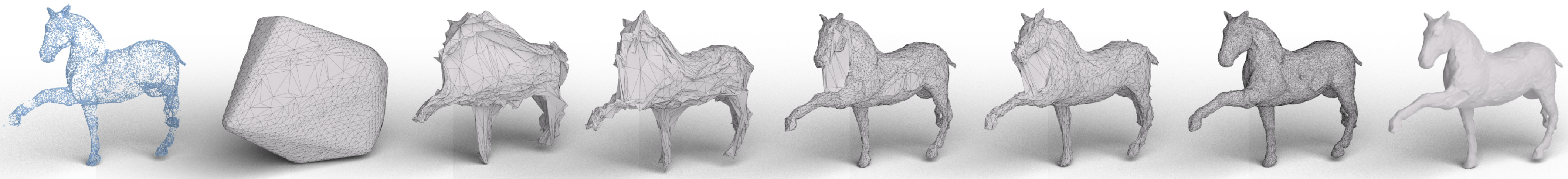
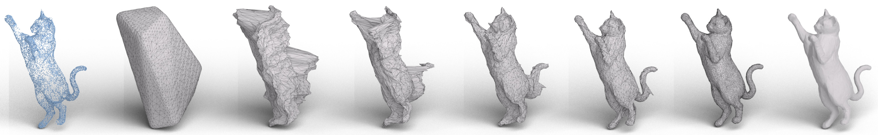
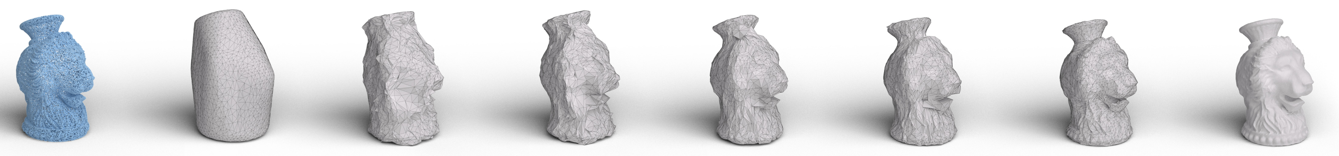
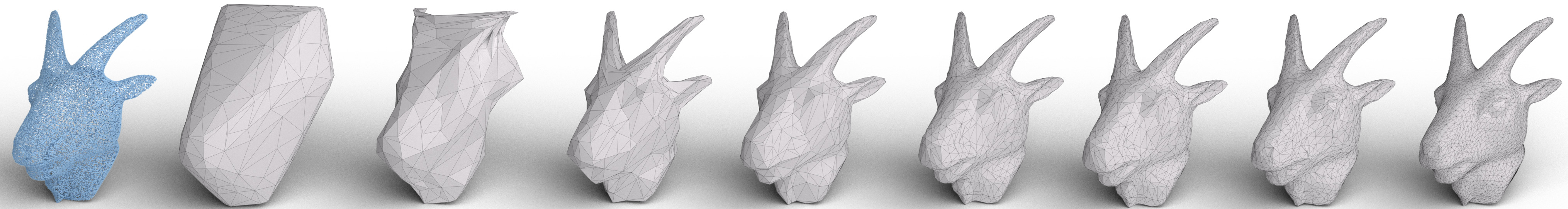
Figure 8. Iterative progression through the Point2Mesh optimization process. Starting with the input point cloud (left), the inital mesh begins to deform towards the input point cloud. The mesh is iteratively upsampled, to add finer details throughout the optimization procedure.

Point2Mesh reconstructs a watertight mesh by optimizing the weights of a CNN to iteratively deform an initial mesh to shrink-wrap the given input point cloud $X$ (examples in Figure 8). The CNN automatically defines the self-prior, which enjoys the innate properties of the network structure. Key to the self-prior is the weight sharing structure of the CNN, which inherently models recurring and correlated structures and, hence, is weak in modeling noise and outliers, which have non-recurring geometries. Natural shapes contain strong self-correlation across multiple-scales and fine-grained details often reoccur, while noise is random and uncorrelated; making reconstructing recurring fine-grained details while eliminating noise possible. Observe Figure 6, where the self-prior removes the noisy bumps on the reoccurring ridges on the Ankylosaurus back and tail, yet still preserves the fine-grained ridges on the neck. Moreover, notice how the self-prior complete the missing portions in Figure 2 and 7 in a manner that is consistent with the characteristic of the global shape. An overview of our approach is illustrated in Figure 4.

We perform the reconstruction in a coarse-to-fine manner, where the output mesh at level $l$ is denoted by $\hat{M}_{l}{}$. The network takes as input a mesh $\hat{M}_{l-1}{}$ and predicts displacements $\Delta\hat{V}_{l}{}$, which move the mesh vertices towards the point cloud, driven by a loss to close the gap between the mesh surface and the point cloud. The convergence is iterative, since the displacements continue to increase to deform the mesh to shrink wrap the point cloud. In each iteration the network receives as input a random noise vector $C_{l}$, and the weights $W_{l}{}$ are randomly initialized. The $C_{l}$ vector serves as a random initialization for the predicted displacements, and the network weights are optimized to minimize the loss, while $C_{l}$ remains constant.

Point2Mesh works in coarse-to-fine levels, where in each level the predicted mesh is refined by subdividing its triangles. The initial mesh is coarse approximation of the point cloud. If the object has a genus of zero we use the convex hull of the point cloud, whereas we use a coarse alpha shape [Edelsbrunner and Mücke, 1994] for shapes with arbitrary genus (alternatively, we can use other methods).

Our network is comprised of a series of edge-based convolution and pooling layers, as originally proposed in MeshCNN. However, unlike MeshCNN, which uses geometric input features, Point2Mesh input features are the entries of the random (fixed) vector $C_{l}$. The convolutional kernels operate on the edges of the input mesh $\hat{M}_{l-1}{}$, initialized by $C_{l}$, and are optimized to predict vertex displacements $\Delta\hat{V}_{l}{}$. Specifically, the edge filters regress a list of displaced mesh edges $\Delta\hat{E}_{l}{}$, where each edge is represented by the three coordinates of both endpoint vertices (dimension $\#E\times 2\times 3$). The location of each vertex in the list of edges is averaged to yield the final list of per-vertex displacements $\Delta\hat{V}_{l}{}$.

Figure 5. Illustration of edge displacements predicted by network (left) and then averaged (right).

Once the displacements $\Delta\hat{V}_{l}{}$ are predicted, the updated mesh $\hat{M}_{l}{}$ is reconstructed, and the loss is computed by measuring the gap between the updated mesh and the point cloud, which drives the optimization of the network filters. Note that since the vertex displacements do not alter the mesh connectivity, the reconstructed mesh $\hat{M}_{l}{}$ has the prescribed connectivity and genus of $\hat{M}_{l-1}{}$.

The input tensor $C_{l}$ has six feature vectors per edge, with the same number of edges as $\hat{M}_{l-1}{}$, sampled from a uniform distribution $[0,1)$. The values of $C_{l}$ are sampled once per level, and remain constant during the optimization process. Effectively, the network acts as a parameterization of the input point cloud $X$ by the network weights and the fixed vector $C_{l}$, i.e., $X=f_{W_{l}{}}(C_{l})$. However, we often do not actually wish to recover $X$ exactly, since it can be corrupted with noise, unoriented normals or missing regions. Setting $C_{l}$ to be random helps the network avoid bias and overfitting.

\begin{overpic}[width=512.1496pt]{figures/06_experiments/068_self_similarity/ankyt.jpg} \put(6.0,-3.0){{\color[rgb]{0,0,0}Ground-Truth}} \put(33.7,-3.0){{\color[rgb]{0,0,0}Input}} \put(55.2,-3.0){{\color[rgb]{0,0,0}Smooth-prior}} \put(81.0,-3.0){{\color[rgb]{0,0,0}Self-prior}} \end{overpic}

Figure 6. The input point cloud is sampled from a (ground-truth) mesh, with added noise and missing regions. A smooth-prior reconstructs the surface locally, oblivious to the global shape. While the self-prior retains the reoccurring ridges in the back of the ankylosaurus and it smooths bumps which originated from noise. Note the smooth reconstruction along the tail and side of the body.

3.1. Explicit Mesh Representation

The reconstructed surface is represented as a triangular mesh. A triangular mesh is defined by a set of vertices, (triangular) faces and edges: ($V$, $F$, $E$), where $V=\left\{\mathbf{v}_{1},\mathbf{v}_{2}\cdots\right\}$ is the set of vertex positions in $\mathbb{R}^{3}$. The connectivity is given by a set of faces $F$ (triplets of vertices), and a set of edges $E=\left\{\mathbf{e}_{1},\mathbf{e}_{2}\cdots\right\}$ (pairs of vertices).

The reconstructed surface $\hat{M}_{l}{}$ is directly deformed by our network. Instead of estimating the absolute vertex position $\hat{V}_{l}{}$ of the deformed mesh, the network estimates a differential vertex position $\Delta\hat{V}_{l}{}$, relative to the input mesh vertices $\hat{V}_{l-1}{}\in\hat{M}_{l-1}{}$ (i.e., $\hat{V}_{l}{}=\hat{V}_{l-1}{}+\Delta\hat{V}_{l}{}$). This facilitates learning in two main ways. First, the last layer in the network can be initialized with zeros (i.e., no displacement), which leads to a better initial condition for the optimization. Second, there is evidence in neural networks that predicting residuals yields more favorable results [Shamir, 2018], especially for tasks which regress displacements [Hanocka et al., 2018].

We use the neural building blocks of MeshCNN to regress the final vertex locations of the predicted mesh. However, since MeshCNN operates on edges, it regresses a list of edge displacements $\Delta\hat{E}_{l}{}$, consisting of pairs of vertex displacements. Since a particular vertex is incident to many edges (i.e., six on average), the final vertex locations must aggregate over all the predicted vertex locations (illustrated in Figure 5). To handle this, the over-determined list of vertex displacements in $\Delta\hat{E}_{l}{}$ is fed into a Build $\Delta V$ module (Figure 4) that creates a unique list of vertex displacements $\Delta\hat{V}_{l}{}$. Specifically, for each vertex, the predicted vertex displacements in each edge are averaged to get the final list of vertices. A particular vertex position $\mathbf{\hat{v}}_{i}$ is calculated by

(1) $$\mathbf{\hat{v}}_{i}=\frac{1}{n}\sum_{j\in n}\mathbf{\hat{e}_{j}}(v_{i}),$$

where $\mathbf{\hat{e}_{j}}(v_{i})$ is the vertex position of $v_{i}$ in edge ${e}_{j}$, and $n$ is the valence of vertex $\mathbf{\hat{v}}_{i}$.

3.2. Mesh to Point Cloud Distance

The estimated mesh vertices are driven by the distance of the deformed mesh $\hat{M}_{l}{}$ to the input point cloud $X$. The deformed mesh $\hat{M}_{l}{}$ is sampled via a (differential) sampling layer resulting in a point set $\hat{Y}$ that is measured against the input point set $X$. We evaluate the distance using the bi-directional Chamfer distance:

(2) $$d(X,\hat{Y})=\sum_{x\in X}\min_{\hat{y}\in\hat{Y}}||x-\hat{y}||_{2}+\sum_{\hat{y}\in\hat{Y}}\min_{x\in X}||x-\hat{y}||_{2},$$

which is fast, differential and robust to outliers [Fan et al., 2017].

To compare the reconstructed mesh to the input point cloud, we sample the mesh surface. Since the network weights encode information, which ultimately predicts the deformed mesh vertex locations, the sampling mechanism must be differential in order to back-propagate gradients through the network weights. A point sampled from a particular triangle has some distance to the closest point in the point cloud. This distance contributes to a gradient update, which will displace the three vertices that define the face of the sampled point. A mesh can be sampled by first selecting a face from a distribution $P_{f}$ and then sampling a point within each triangle from another distribution $P_{p}$. We use a uniform sampler, where the area of each triangle is proportional to the probability of selecting it $P_{f}\propto A_{f}$. Uniformly sampling a point inside a triangle with vertices $v_{0},v_{1},v_{2}$ (where $v_{0}$ is at the origin), is given by ${a_{1}\cdot v_{1}+a_{2}\cdot v_{2}}$ (where $a_{1}$ and $a_{2}$ are $\in U(0,1)$ and $a_{1}+a_{2}<1$).

\begin{overpic}[width=433.62pt]{figures/06_experiments/068_self_similarity/flat_missing.jpg} \put(12.0,-3.0){{\color[rgb]{0,0,0}Input}} \put(31.0,-3.0){{\color[rgb]{0,0,0}Smooth-prior}} \put(68.0,-3.0){{\color[rgb]{0,0,0}Self-prior}} \end{overpic}

Figure 7. Point2Mesh exploits self similarity in order to reconstruct a better missing half dome.

3.3. Beam-Gap Loss

Deforming a mesh to enter narrow and deep cavities is a difficult task. Specifically, a mesh optimization which only uses the bi-directional Chamfer distance can become trapped in a local minimum, without ever entering the cavity. To drive the mesh into deep cavities, we calculate beam rays, from the mesh to the input point cloud, which we call beam-gap. Calculating the exact beam-gap intersection is not possible, since the input point cloud is a sparse and discrete representation of a continuous surface. Therefore, we propose a method for approximating the distance to the underlying surface, which serves as an additional loss to the Chamfer loss.

For a point $\hat{y}$ sampled from a deformable mesh face, a beam is cast in the direction of the deformable face normal. The beam intersection with the point cloud is the closest point in an $\epsilon$ cylinder around the beam. More formally, the beam intersection (or collision) of a point $\hat{y}$ is given by $\mathcal{B}(\hat{y})=x$, and so the overall beam-gap loss is given by:

(3) $$\mathcal{L}_{b}(X,\hat{Y})=\sum_{\hat{y}\in\hat{Y}}\left\lVert{\hat{y}-\mathcal{B}(\hat{y})}\right\rVert^{2}.$$

Since the underlying surface of the target shape is unknown, the beam-gap distance is a discrete approximation of the true beam intersection. Our system is not sensitive to the selection of $\epsilon$ (used $\epsilon=0.99$), assuming a reasonable sampling density.

Note, that not all points on the reconstructed mesh obtain a beam collision to the point cloud. In this case, the beam-gap of $\mathcal{B}(\hat{y})=\hat{y}$ (i.e., no penalty). Furthermore, if multiple beam intersections are detected, we select the closest one. If for a given point sampled from the reconstructed mesh there is a good fit to the target point cloud, then there is no beam-gap penalty for this point. We determine areas with a good fit by computing the mutual $k$-Nearest Neighbor ($k$-NN) between $\hat{y}$ and all the points in the target point cloud $X$. In other words, if any of the $k$-NN of $\hat{y}$ to $X$ also have $\hat{y}$ in any of their $k$-NN, then the point $\hat{y}$ already has a good fit and does not receive a beam-gap penalty.

4. Implementation Details

4.1. Iterative Coarse-to-Fine Optimization

The optimization process has two main coarse-to-fine aspects: (i) periodically up-sampling the mesh resolution (i.e., number of mesh elements); and (ii) increasing the number of point samples taken from the reconstructed mesh.

Mesh subdivision, in the context of Point2Mesh, has two main purposes: enabling the expression of richer and finer geometric details, and allowing the optimization to move away from local minima. Finer meshes are more flexible, since they can easily move toward their target. However, starting with a large mesh resolution will inevitably over-complicate the optimization process. To this end, the initial mesh starts out with a relatively small number of faces (roughly a couple thousand), and the optimization begins to move the mesh vertices to achieve a rough alignment of the starting mesh with the target point cloud. As the optimization progresses, the mesh is subdivided and smoothed, as it continues to deform into the target shape.

During the coarse optimization iterations, we upsample the mesh using the robust watertight manifold surface generation of Huang et al. [2018], which we will refer to as $\mathsf{RWM}$. First, the network weights update and start to deform the initial coarse mesh to move toward the target. After $K$ optimization iterations (a hyperparameter, we use $K=1000$), the current deformed mesh is passed to $\mathsf{RWM}$. The new $\mathsf{RWM}$-generated mesh is a manifold, watertight and non-intersecting surface, which is used as the initial mesh to the next level of optimization. We use a high octree resolution (i.e., number of leaf nodes) in $\mathsf{RWM}$, to preserve the details recovered in the optimization and also introduce more polygons. The number of polygons in the $\mathsf{RWM}$-output will be simplified to the target number of faces that we pre-defined for the next optimization iteration. In practice, we increase the number of faces by $1.5$ after reaching the end of an optimization, and stop increasing the resolution once the maximum number of faces is met. Note that the weights and the constant random vector $C$ are re-initialized at the beginning of each optimization level.

The second aspect in the coarse-to-fine optimization is the number of points that are sampled on the reconstructed mesh. Initially, over-sampling the reconstructed mesh with too many points may significantly slow down the optimization process, since different points sampled from the same mesh face may (initially) be driven to vastly different directions by the loss function. To facilitate desirable convergence, we iteratively increase the number of reconstructed mesh point samples in each level of optimization. Specifically, we pre-define: the number of starting samples $R_{0}$ (usually $R_{0}=15$k) and a final number of samples $R_{K}$. The number of reconstructed mesh samples increases linearly until reaching the maximum number $R_{K}$ after $K$ optimization iterations. After moving to the next optimization level, we restart the number of samples to $R_{0}$. For intricate shapes, we sample a maximum of  $50$k-$100$k points, while simpler shapes require around $15$k-$30$k points.

The manifold surface generation helps the optimization in two ways. First, creating a clean non-intersecting surface makes it simpler for the optimization to displace the mesh vertex positions. Secondly, since it uses an octree to reconstruct the surface, the upsampled mesh has relatively uniformly sized triangles, which helps large flat areas that cover unentered cavities contain enough resolution to deform. The watertight manifold implementation is relatively fast, taking $10.5$ seconds on a single GTX 2080 TI GPU for a mesh with 40,000 triangles using 20,000 leaf nodes in the octree.

4.2. Part-Based

The GPU memory needed to optimize a given mesh increases as the mesh resolution increases. To alleviate this problem (at finer resolutions), a PartMesh data structure is defined, which enables the entire mesh to be optimized by parts. A PartMesh is a collection of sub-meshes which together make up the complete mesh.

Given a reconstructed mesh $\hat{M}$, a PartMesh representing $\hat{M}$ will have a set of sub-meshes, where each contains a subset of the vertices and faces from $\hat{M}$. Once defined, the architecture of our network can be manipulated to receive a PartMesh as input, performing a forward pass on each part separately, accumulating the gradients for the entire mesh $\hat{M}$, and then performing back-propagation once using all the accumulated gradients. The final mesh reconstruction $\hat{M}$ can then be recovered from the PartMesh.

Moreover, we enable overlapping regions between different sub-meshes in the PartMesh. In the case that a particular vertex is present in more than one sub-mesh, the final vertex position will be the average over all of the locations in each sub-mesh. The mesh is divided into sub-parts by splitting the vertices into an $n\times n$ grid.

4.3. Initial Mesh Approximation

Depending on the requirements of the reconstruction, we can use different methods for approximating the initial deformable mesh. For shapes known to have genus-0, we use the convex hull as the initial mesh. If the genus is unknown or greater than 0, we approximate the initial mesh through a series of steps. First, we calculate the the alpha shape or Poisson reconstruction from the input point cloud. Then, we apply the watertight manifold algorithm [Huang et al., 2018] using a very coarse resolution octree (on the order of a few hundred leaf nodes).

This coarse approximation has two main purposes: (i) it distances the initial mesh from potentially incorrect reconstructions, which are the result of noise, low-density regions, or incorrect normals (in the case of Poisson) and (ii) it helps close topologically incorrect holes that might occur in low-density regions (e.g., Figure 9).

\begin{overpic}[width=241.84842pt]{figures/06_experiments/069_genus/0399.jpg} \put(8.0,-3.0){{\color[rgb]{0,0,0}Input}} \put(36.0,-3.0){{\color[rgb]{0,0,0}Poisson}} \put(58.0,-3.0){{\color[rgb]{0,0,0}Initial}} \put(75.0,-3.0){{\color[rgb]{0,0,0}Self-prior}} \end{overpic}

Figure 9. Arbitrary genus with missing portions. Starting with the input point cloud, Poisson reconstruction results in incorrect topological holes. We apply a low resolution octree tree to close incorrect holes and create a coarse initial mesh which is used as the initial mesh. The result of Point2Mesh is a topologically correct mesh which preserves the details from the input point cloud, and does not overfit to incorrect low density regions (note the top of the chair).

\begin{overpic}[width=433.62pt]{figures/noisy/harmonics.jpg} \put(10.0,-3.0){{\color[rgb]{0,0,0}Input}} \put(35.0,-3.0){{\color[rgb]{0,0,0}DGP}} \put(52.0,-3.0){{\color[rgb]{0,0,0}DGP+Poisson}} \put(81.0,-3.0){{\color[rgb]{0,0,0}Self-Prior}} \end{overpic}

Figure 10. Surface reconstruction on noisy input with self-repetitions. Sampling the local DGP charts which are passed as input to Poisson (which struggles with unoriented normals).

4.4. Run-time

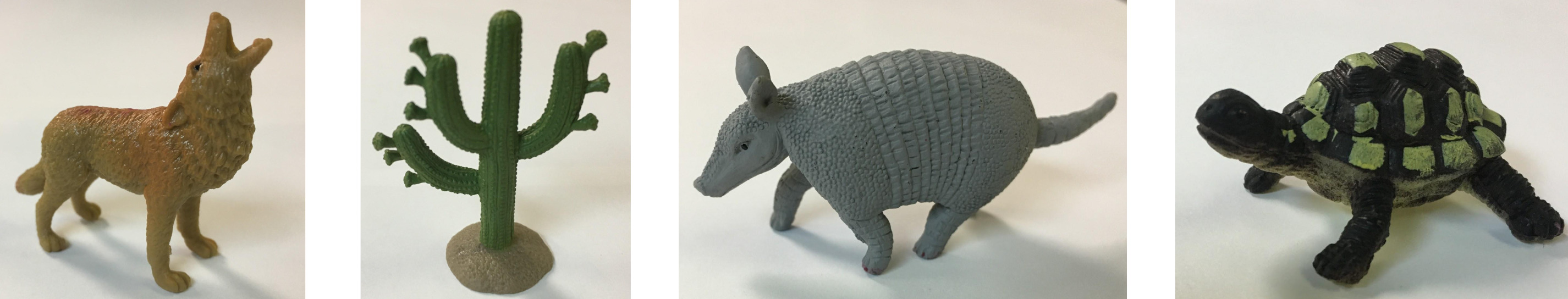
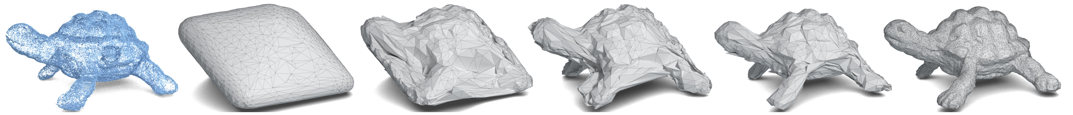
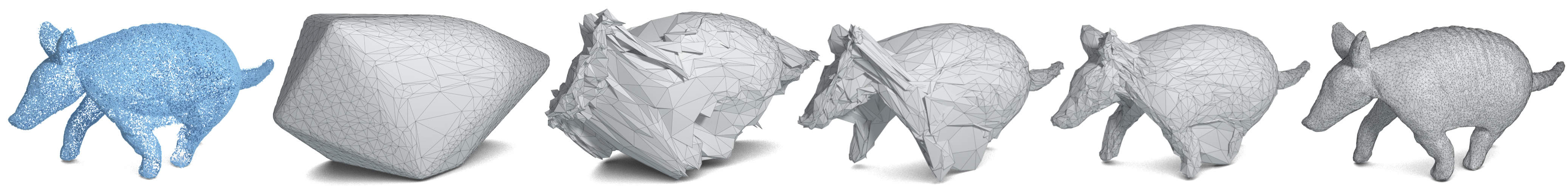
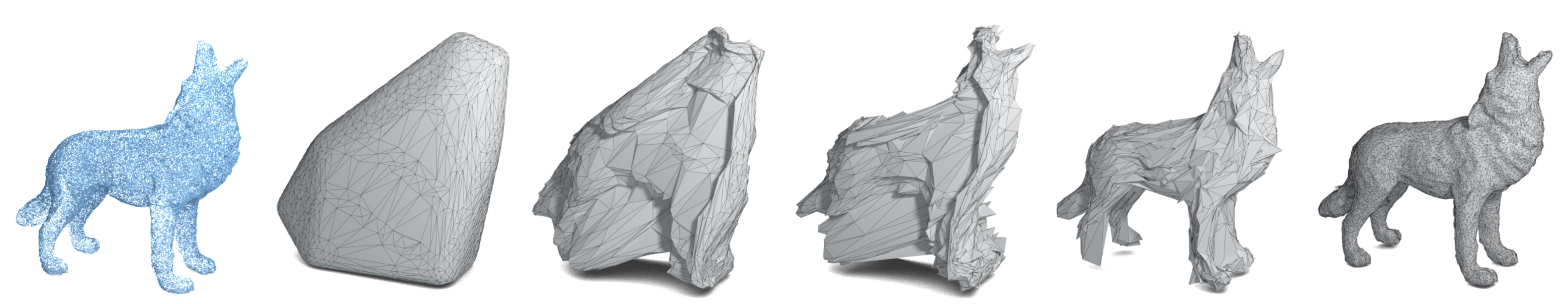
Figure 11. Mesh reconstruction process of four objects (top row) scanned using NextEngine 3D laser scanner.

The speed of our non-optimized PyTorch [Paszke et al., 2017] implementation is a function of mesh resolution and number of samples. An iteration (forward and backward pass) takes $0.23$ seconds for a mesh with 2,000 faces and 15,000 points in the target and reconstructed mesh, or $0.59$ seconds for a mesh with 6,000 faces using a GTX 1080 TI graphics card. For a mesh with 40,000 faces (using $8$ parts), it takes $4.7$ seconds per iteration (i.e., $0.59$ seconds per part). The number of iterations required varies according to the complexity of the model, where simple models can converge in less than 1,000 iterations, while more complex ones may need around 10,000 (or more) iterations. Therefore, depending on the complexity, the total runtime for most models can range anywhere from a few ($\sim 3$) minutes to several ($\sim 3$) hours. While extremely high resolution results can take over 14 hours. A table with the runtimes for each of the models is listed in the supplementary material.

5. Experiments

We validate the applicability of Point2Mesh through a series of qualitative and quantitative experiments involving shapes with missing regions, noise and challenging cavities. We start with qualitative results of our method on real scanned objects from [Choi et al., 2016] as well as from the NextEngine 3D laser scanner. We provide additional results and quantitative experiments on point sets sampled from a ground-truth mesh surface. These mesh datasets include: Thingi10k [Zhou and Jacobson, 2016], COSEG [Wang et al., 2012], TOSCA high-resolution [Bronstein et al., 2006] and the Surface Reconstruction Benchmark [Berger et al., 2013].

\begin{overpic}[width=426.79134pt]{figures/06_experiments/065_unoriented/triceratops.jpg} \put(12.0,-2.0){{\color[rgb]{0,0,0}Input}} \put(44.0,-2.0){{\color[rgb]{0,0,0}Poisson}} \put(78.0,-2.0){{\color[rgb]{0,0,0}Ours}} \end{overpic}

Figure 12. Reconstruction results on estimated normals. Calculating normals on the input point cloud and applying a normal orientation algorithm (heat map colors of error angle to ground-truth normal). While Screened Poisson is sensitive to unoriented normals, Point2Mesh is agnostic to orientation.

\begin{overpic}[width=241.84842pt]{figures/06_experiments/064_choi_scan/choi_scans.jpg} \put(12.0,-3.0){{\color[rgb]{0,0,0}Input}} \put(41.0,-3.0){{\color[rgb]{0,0,0}Poisson}} \put(72.0,-3.0){{\color[rgb]{0,0,0}Self-prior}} \end{overpic}

Figure 13. Reconstruction from real scans from [Choi et al., 2016]. Note that Point2Mesh guarantees reconstruction of a watertight surface despite noise, missing regions and unoriented normals.

5.1. Real Scans

Before presenting our results on real scans, we discuss the problem of imperfect normals, which is a characteristic of real scanned data. While our method uses the normal information provided in the point cloud, as we demonstrate below, it is robust to noisy and inaccurate normals. This is due to the small weight on the normal penalty (cosine similarity) and the self-prior.

Normal Estimation

Generally, in ideal conditions, points uniformly sample the shape, are noise-free, have correct / oriented normals and have sufficient resolution. Under such ideal conditions, a smooth-prior (e.g., Poisson reconstruction) is an excellent choice for reconstruction. An advantage of Point2Mesh compared to smooth-priors is the ability to cope with unoriented normals. Meaning the line defining the normal is correct, however, the direction (inward or outward) may be be incorrect. If normals are unoriented (or overly noisy), it is a rather challenging task to correctly orient them with existing tools.

To evaluate the orientation problem, we sample a mesh without normals, and estimate the normals and their orientation using [Zhou et al., 2018]. The results of our approach are presented in Figure 12. The input point cloud is visualized with a heatmap of the angle of the estimated normal error, and the results of Screened Poisson reconstruction and Point2Mesh are displayed side-by-side. Note that the loss function that we use aims to align the normals of the input point cloud and its corresponding point in the mesh using a cosine similarity. In the event that the normals are unoriented, we use the absolute dot-product between the two vectors, which gives equal penalty for vectors $180^{\circ}$ out of phase.

NextEngine 3D scans

We have scanned four objects using the NextEngine 3D laser scanner and show the reconstruction results and iterative convergence in Figure 11. The second column to the left shows the initial mesh, which is the convex hull. Observe that despite the large holes in the input point cloud, Point2Mesh results in a plausible reconstruction.

Choi et al. [2016] scans

Figure 13 demonstrates the reconstruction from real scans obtained from [Choi et al., 2016]. Not all normals in these scans are oriented to the correct direction, and the smooth reconstruction therefore has some observable artifacts which are not present in Point2Mesh results.

5.2. Accuracy Metric

For a quantitative comparison, we evaluate Point2Mesh on a point cloud obtained from a ground-truth mesh. For the metric between the ground-truth and the reconstructed mesh, we use the F-score metric as discussed in Knapitsch et al. [2017]. The F-score is defined by the precision $P(\tau)$ and recall $R(\tau)$ at a given distance threshold $\tau$. The precision can be thought of as some type of accuracy of the reconstruction, which considers the distance from the reconstructed mesh to ground-truth mesh. The recall provides an indication of how well the reconstructed mesh covers the target shape, which considers the distance from the ground-truth mesh to the reconstructed mesh. The F-score $F(\tau)$ is the harmonic mean between $P(\tau)$ and $R(\tau)$. The best F-score is $100$ and the worst is $0$. For more details about the F-score, refer to the supplementary material. It is worth noting that like all distortion-based metrics for inverse problems, a high F-score may not necessarily imply better visual quality, and vice-versa [Blau and Michaeli, 2018].

Table 1. Shape denoising comparison. F-score (larger is better) statistics for five different noise samples of each underlying shape.

	Guitar				Tiki
Method	avg	std	min	max	avg	std	min	max
Poisson	86.4	2.6	82.5	89.1	47.6	0.3	47.2	47.9
PCN	97.2	1.0	95.8	98.3	58.6	0.4	57.8	59.1
DGP	92.9	1.3	90.9	94.2	50.7	0.7	49.8	51.9
Ours	98.3	0.5	97.5	98.8	60.2	0.4	59.6	60.6

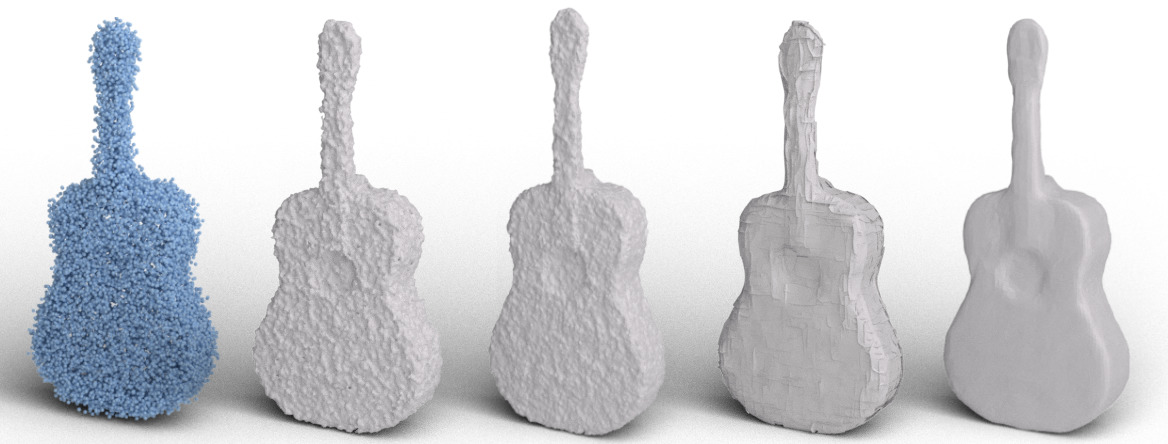
\begin{overpic}[width=241.84842pt]{figures/06_experiments/060_noise_benchmark/noise_tiki.jpg} \put(8.0,-3.0){{\color[rgb]{0,0,0}Input}} \put(25.0,-3.0){{\color[rgb]{0,0,0}Poisson}} \put(45.0,-3.0){{\color[rgb]{0,0,0}PCN}} \put(68.0,-3.0){{\color[rgb]{0,0,0}DGP}} \put(86.0,-3.0){{\color[rgb]{0,0,0}Ours}} \end{overpic}

Figure 14. Qualitative results from the noisy comparison.

5.3. Comparisons

Denoising

To evaluate our approach on the task of denoising, we use two meshes as ground-truth for performing quantitative comparisons. We sample each mesh with $75,000$ points and add a small amount of Gaussian noise to each $<x,y,z>$ coordinate in the input point cloud. We sample from the noise distribution five times per shape and report F-score statistics for the five versions of each shape in Table 1. Qualitative examples are shown in Figure 14.

We compare against Screen Poisson surface reconstruction [2013], DGP [2019] and PointCleanNet (PCN) [2019], which trains a neural network directly for the task of point cloud denoising. Note that we apply a Poisson reconstruction on the result of PCN for the sake of visualizing their result, but the F-score is computed on the raw (cleaned) point samples. We use the same configuration for each method across all shapes. Note that the deep neural network based approaches outperform the classic Poisson smooth-prior. A qualitative comparison on noisy data for a shape with self-repetition is shown in Figure 10. The local charts generated by DGP are sampled and used as input to Poisson.

\begin{overpic}[width=241.84842pt]{figures/06_experiments/063_inpaintint_benchmark/inpaint_giraffe.jpg} \put(10.0,-2.5){{\color[rgb]{0,0,0}Input}} \put(29.0,-2.5){{\color[rgb]{0,0,0}Poisson}} \put(50.0,-2.5){{\color[rgb]{0,0,0}PCN}} \put(69.0,-2.5){{\color[rgb]{0,0,0}DGP}} \put(87.0,-2.5){{\color[rgb]{0,0,0}Ours}} \end{overpic}

Figure 15. Qualitative results on shape completion comparison.

Low Density Completion

To evaluate our approach on the task of shape completion, we use two meshes as ground-truth for performing quantitative comparisons. In this task, we aim to complete the missing parts of a shape, which contains large regions with very little to no samples. In order to acquire such data, the input point cloud was sampled from meshes where several large random regions were removed. We define a probability for: the number and size of the low-density regions and the frequency for sampling inside them.

We sample the missing region probabilities five times per shape and report statistics for the five versions of each shape in Table 2. Qualitative examples are shown in Figure 15. In the case of completion, we modify the ground-truth used in the F-score computation to better reflect how well the missing regions were completed. The precision component remains with respect to the entire ground-truth surface, while the recall is with respect to the (ground-truth) missing portion of the surface only. Since recall gives some notion of coverage, this indicates how well the missing regions were covered. Note that since we used the convex-hull as the initial mesh, this implicitly provides the correct genus to our approach. In this sense, the comparison is not entirely fair, since the other approaches cannot use this information which provides an advantage for hole filling.

Table 2. Shape completion comparison. F-score (higher is better) statistics for different missing portions of the underlying shape ($\times 5$ per shape). The precision is reported for the entire shape, while the recall is with respect to the missing portion only.

	Giraffe				Bull
Method	avg	std	min	max	avg	std	min	max
Poisson	58.3	12.4	41.2	74.4	84.9	1.6	82.8	87.4
PCN	58.3	12.5	41.3	74.4	84.5	1.7	82.3	87.2
DGP	63.3	13.6	42.6	76.4	75.7	2.9	71.6	80.3
Ours	80.7	11.5	58.2	90.8	87.4	2.8	83.5	92.0

5.4. Network is a Prior

\begin{overpic}[width=241.84842pt]{figures/06_experiments/061_G_convergence/G.jpg} \put(2.0,22.0){{\color[rgb]{0,0,0}(a)}} \put(2.0,5.0){{\color[rgb]{0,0,0}(b)}} \put(20.0,22.0){{\color[rgb]{0,0,0}(c)}} \put(20.0,5.0){{\color[rgb]{0,0,0}(d)}} \end{overpic}

Figure 16. Network is a prior. Starting with the initial mesh (a) and the target point cloud (b), the iterative Point2Mesh convergence is shown along the upper row (c). Optimizing the same objective directly without a network gets trapped in a local minimum (d).

In order to separate the effect of the proposed reconstruction criteria and coarse-to-fine framework from the effect of the self-prior (i.e., network weights), we run an ablation to demonstrate the importance of the network. We optimize the same criteria directly through back-propagation in the same coarse-to-fine fashion (without a network). We call this setting direct optimization, since it directly computes the ideal deformable mesh vertex placements given the same criteria, through back-propagation.

Figure 16 shows that the self-prior (provided by the network) plays a crucial role in facilitating a desirable convergence: The proposed objective for reconstruction (i.e, Chamfer and beam-gap), in addition to our coarse to fine framework (i.e., iterative subdivision) are not sufficient alone to generate the desirable results. This indicates that while a direct optimization approach is prone to local minima, the network as a prior can avoid these minimas by its weight sharing and self similarity capabilities.

Our network architecture is a U-Net configuration with residual and skip connections. The network hyper-parameters define the representational power of the self-prior. This translates to the effectiveness of the self-prior, since a powerful network architecture should lead to a strong self-prior. While the notion of what makes a neural network effective is somewhat obscure, empirically neural networks tend to work poorly in under-parameterized settings (i.e., with not enough trainable weights). To test this, we ran $50$ configurations of the self-prior hyperparameters and manually classified the results as either a noisy or detailed on the centaur shape (Figure 17). We present the average of various parameters from each of the classes in the table below. The clean class was generated from

	noisy	detailed
F-score	81.24%	99.9%
feat	11.6	97.8
minfeat	4	21.6
params	6.5k	263k
pool	40%	20%
res	1.9	2

configurations with more deep features in the bottleneck of the U-Net architecture (feat) and a larger number of learned parameters (params). Narrowing the convolutional width (minfeat) results in noisy reconstructions. Moreover, pooling (pool) less features also seemed to improve performance, while the number of residual connections (res) did not seem to have an effect. Note that we observed empirically, specifically for the task of shape completion, that increased pooling had a more desirable outcome with respect to completion.

\begin{overpic}[width=241.84842pt]{figures/06_experiments/064_cent_prior/cent_prior.jpg} \put(6.0,-3.0){{\color[rgb]{0,0,0}Input}} \put(26.0,-3.0){{\color[rgb]{0,0,0}Optimization}} \put(51.0,-3.0){{\color[rgb]{0,0,0}Over-param}} \put(76.0,-3.0){{\color[rgb]{0,0,0}Under-param}} \end{overpic}

Figure 17. Representational power of network priors. Deforming a mesh to the input point cloud using direct optimization (no network prior) leads to undesirable results. Point2Mesh relies on the representation power of deep CNNs to deform the input mesh, i.e., an overparameterized (Over-param) network, where as an underparameterized (Under-param) network is not expressive enough to produce favorable results.

6. Discussion

The rapid emergence of neural networks has had a tremendous impact in the development of graphical processing, in particular for images, videos, volumes and other regular representations. The use of neural networks on irregular structures is still an open research problem. Most of the research has focused on point clouds, with only a few operating directly on irregular meshes, which focused on analysis only. In this work, we developed a neural network to perform a regression task, which optimizes the geometry of an irregular mesh. The network learns to displace the vertices of the given mesh in the context of surface mesh reconstruction. Moreover, the strategy of deforming a given mesh preserves the genus and provides control, which is lacking in competing methods.

The key point of our presented method is that reconstruction is based on a self-prior that is learned during the mesh optimization itself, and enjoys the innate properties of the network structure, which we refer to as the self-prior. Central to the self-prior is the weight-sharing structure of a CNN, which inherently models recurring and correlated structures and, hence, is weak in modeling noise and outliers, which have non-recurring geometries. Fortunately, natural shapes have strong self-correlation across multiple scales. Their surface is typically piecewise smooth or may contain geometric textures which consist of recurring elements (e.g., most notable in Figures 1, 2, 6, 7). Thus, this self-prior excels in learning and modeling natural shapes, and, in a sense, is magical in completing missing parts and removing outliers or noise.

We demonstrate the applicability of our reconstruction method on imperfect point clouds that are noisy and have missing regions, and show that it performs well in the tasks of denoising and completion. Despite these promising findings, we note the current limitations of our approach: akin to most optimization techniques, our method is quite expensive in terms of time and memory, compared to state-of-the-art surface reconstruction techniques. Furthermore, although we demonstrate handling shapes with genus greater than zero, we had to rely on available techniques which may produce an initial mesh with imperfect results, especially in scenarios with non-ideal conditions.

An interesting direction for future work, could involve developing a separate network that can detect the genus of point cloud without relying on training data: following our approach to learn a self-prior while processing the input data. Another interesting avenue coulbe involve exploring the possibility of using our approach to obtain compatible triangulations between shapes, for example, by optimizing the same deformable mesh to shrink-wrap two or more different objects.

- [1]
- Achille and Soatto [2018] Alessandro Achille and Stefano Soatto. 2018. Emergence of invariance and disentanglement in deep representations. The Journal of Machine Learning Research 19, 1 (2018), 1947–1980.
- Berger et al. [2013] Matthew Berger, Joshua A Levine, Luis Gustavo Nonato, Gabriel Taubin, and Claudio T Silva. 2013. A benchmark for surface reconstruction. ACM Transactions on Graphics (TOG) 32, 2 (2013), 20.
- Berger et al. [2017] Matthew Berger, Andrea Tagliasacchi, Lee M Seversky, Pierre Alliez, Gael Guennebaud, Joshua A Levine, Andrei Sharf, and Claudio T Silva. 2017. A survey of surface reconstruction from point clouds. In Computer Graphics Forum, Vol. 36. Wiley Online Library, 301–329.
- Blau and Michaeli [2018] Yochai Blau and Tomer Michaeli. 2018. The perception-distortion tradeoff. In Proceedings of the IEEE Conference on Computer Vision and Pattern Recognition. 6228–6237.
- Bronstein et al. [2006] Alexander M Bronstein, Michael M Bronstein, and Ron Kimmel. 2006. Efficient computation of isometry-invariant distances between surfaces. SIAM Journal on Scientific Computing 28, 5 (2006), 1812–1836.
- Bronstein et al. [2017] Michael M Bronstein, Joan Bruna, Yann LeCun, Arthur Szlam, and Pierre Vandergheynst. 2017. Geometric deep learning: going beyond euclidean data. IEEE Signal Processing Magazine 34, 4 (2017), 18–42.
- Chen et al. [2019] Wenzheng Chen, Jun Gao, Huan Ling, Edward Smith, Jaakko Lehtinen, Alec Jacobson, and Sanja Fidler. 2019. Learning to Predict 3D Objects with an Interpolation-based Differentiable Renderer. In Advances In Neural Information Processing Systems.
- Choi et al. [2016] Sungjoon Choi, Qian-Yi Zhou, Stephen Miller, and Vladlen Koltun. 2016. A Large Dataset of Object Scans. arXiv:1602.02481 (2016).
- Dai and Nießner [2019] Angela Dai and Matthias Nießner. 2019. Scan2mesh: From unstructured range scans to 3d meshes. In CVPR. 5574–5583.
- Edelsbrunner and Mücke [1994] Herbert Edelsbrunner and Ernst P Mücke. 1994. Three-dimensional alpha shapes. ACM Transactions on Graphics (TOG) 13, 1 (1994), 43–72.
- Fan et al. [2017] Haoqiang Fan, Hao Su, and Leonidas J Guibas. 2017. A point set generation network for 3d object reconstruction from a single image. In Proceedings of the IEEE conference on computer vision and pattern recognition. 605–613.
- Gaier and Ha [2019] Adam Gaier and David Ha. 2019. Weight Agnostic Neural Networks. arXiv:1906.04358 (2019).
- Gandelsman et al. [2019] Yossi Gandelsman, Assaf Shocher, and Michal Irani. 2019. ”Double-DIP”: Unsupervised Image Decomposition via Coupled Deep-Image-Priors. (6 2019).
- Gao et al. [2019] Lin Gao, Jie Yang, Tong Wu, Yu-Jie Yuan, Hongbo Fu, Yu-Kun Lai, and Hao Zhang. 2019. SDM-NET: Deep generative network for structured deformable mesh. ACM Transactions on Graphics (TOG) 38, 6 (2019), 1–15.
- Groueix et al. [2018] Thibault Groueix, Matthew Fisher, Vladimir G Kim, Bryan C Russell, and Mathieu Aubry. 2018. A papier-mâché approach to learning 3d surface generation. In Proceedings of the IEEE conference on computer vision and pattern recognition. 216–224.
- Hanocka et al. [2018] Rana Hanocka, Noa Fish, Zhenhua Wang, Raja Giryes, Shachar Fleishman, and Daniel Cohen-Or. 2018. ALIGNet: partial-shape agnostic alignment via unsupervised learning. ACM Transactions on Graphics (TOG) 38, 1 (2018), 1. https://doi.org/10.1145/3267347
- Hanocka et al. [2019] Rana Hanocka, Amir Hertz, Noa Fish, Raja Giryes, Shachar Fleishman, and Daniel Cohen-Or. 2019. MeshCNN: A Network with an Edge. ACM Trans. Graph. 38, 4, Article 90 (July 2019), 12 pages. https://doi.org/10.1145/3306346.3322959
- Harary et al. [2014] Gur Harary, Ayellet Tal, and Eitan Grinspun. 2014. Context-based coherent surface completion. ACM Transactions on Graphics (TOG) 33, 1 (2014), 1–12.
- Hoppe et al. [1992] Hugues Hoppe, Tony DeRose, Tom Duchamp, John McDonald, and Werner Stuetzle. 1992. Surface Reconstruction from Unorganized Points. SIGGRAPH Comput. Graph. 26, 2 (July 1992), 71–78. https://doi.org/10.1145/142920.134011
- Hornung and Kobbelt [2006] Alexander Hornung and Leif Kobbelt. 2006. Robust reconstruction of watertight 3 d models from non-uniformly sampled point clouds without normal information. In Symposium on geometry processing. Citeseer, 41–50.
- Huang et al. [2009] Hui Huang, Dan Li, Hao Zhang, Uri Ascher, and Daniel Cohen-Or. 2009. Consolidation of unorganized point clouds for surface reconstruction. ACM transactions on graphics (TOG) 28, 5 (2009), 176.
- Huang et al. [2013] Hui Huang, Shihao Wu, Minglun Gong, Daniel Cohen-Or, Uri Ascher, and Hao Richard Zhang. 2013. Edge-aware point set resampling. ACM transactions on graphics (TOG) 32, 1 (2013), 9.
- Huang et al. [2018] Jingwei Huang, Hao Su, and Leonidas Guibas. 2018. Robust Watertight Manifold Surface Generation Method for ShapeNet Models. arXiv:1802.01698 (2018).
- Kass et al. [1988] Michael Kass, Andrew Witkin, and Demetri Terzopoulos. 1988. Snakes: Active contour models. International journal of computer vision 1, 4 (1988), 321–331.
- Kazhdan [2005] Michael Kazhdan. 2005. Reconstruction of solid models from oriented point sets. In Eurographics symposium on Geometry processing. Eurographics Association, 73.
- Kazhdan et al. [2006] Michael Kazhdan, Matthew Bolitho, and Hugues Hoppe. 2006. Poisson surface reconstruction. In Eurographics symposium on Geometry processing, Vol. 7.
- Kazhdan and Hoppe [2013] Michael Kazhdan and Hugues Hoppe. 2013. Screened poisson surface reconstruction. ACM Transactions on Graphics (ToG) 32, 3 (2013), 29.
- Knapitsch et al. [2017] Arno Knapitsch, Jaesik Park, Qian-Yi Zhou, and Vladlen Koltun. 2017. Tanks and Temples: Benchmarking Large-Scale Scene Reconstruction. ACM Transactions on Graphics 36, 4 (2017).
- Kurenkov et al. [2018] Andrey Kurenkov, Jingwei Ji, Animesh Garg, Viraj Mehta, JunYoung Gwak, Christopher Choy, and Silvio Savarese. 2018. Deformnet: Free-form deformation network for 3d shape reconstruction from a single image. In WACV. IEEE, 858–866.
- Li et al. [2010] Guo Li, Ligang Liu, Hanlin Zheng, and Niloy J Mitra. 2010. Analysis, reconstruction and manipulation using arterial snakes. ACM Trans. Graph. 29, 6 (2010), 152.
- Li et al. [2019] Ruihui Li, Xianzhi Li, Chi-Wing Fu, Daniel Cohen-Or, and Pheng-Ann Heng. 2019. PU-GAN: a Point Cloud Upsampling Adversarial Network. In IEEE International Conference on Computer Vision (ICCV).
- Lipman et al. [2007] Yaron Lipman, Daniel Cohen-Or, David Levin, and Hillel Tal-Ezer. 2007. Parameterization-free projection for geometry reconstruction. In ACM Transactions on Graphics (TOG), Vol. 26. ACM, 22.
- Manson et al. [2008] Josiah Manson, Guergana Petrova, and Scott Schaefer. 2008. Streaming surface reconstruction using wavelets. In Computer Graphics Forum, Vol. 27. Wiley Online Library, 1411–1420.
- McInerney and Terzopoulos [2000] Tim McInerney and Demetri Terzopoulos. 2000. T-snakes: Topology adaptive snakes. Medical image analysis 4, 2 (2000), 73–91.
- Miao et al. [2009] Yongwei Miao, Pablo Diaz-Gutierrez, Renato Pajarola, M Gopi, and Jieqing Feng. 2009. Shape isophotic error netric controllable re-sampling for point-sampled surfaces. In International Conference on Shape Modeling and Applications. IEEE, 28–35.
- Nagai et al. [2009] Yukie Nagai, Yutaka Ohtake, and Hiromasa Suzuki. 2009. Smoothing of partition of unity implicit surfaces for noise robust surface reconstruction. In Computer Graphics Forum, Vol. 28. Wiley Online Library, 1339–1348.
- Nan et al. [2010] Liangliang Nan, Andrei Sharf, Hao Zhang, Daniel Cohen-Or, and Baoquan Chen. 2010. Smartboxes for interactive urban reconstruction. In ACM SIGGRAPH 2010. 1–10.
- Ohtake et al. [2003] Yutaka Ohtake, Alexander Belyaev, and Hans-Peter Seidel. 2003. A multi-scale approach to 3D scattered data interpolation with compactly supported basis functions. In 2003 Shape Modeling International. IEEE, 153–161.
- Ohtake et al. [2005] Yutaka Ohtake, Alexander Belyaev, and Hans-Peter Seidel. 2005. 3D scattered data interpolation and approximation with multilevel compactly supported RBFs. Graphical Models 67, 3 (2005), 150–165.
- Öztireli et al. [2010] A. Cengiz Öztireli, Marc Alexa, and Markus Gross. 2010. Spectral sampling of manifolds. In ACM SIGGRAPH Asia 2010 papers (SIGGRAPH ASIA ’10). ACM, New York, NY, USA, Article 168, 8 pages. https://doi.org/10.1145/1866158.1866190
- Paszke et al. [2017] Adam Paszke, Sam Gross, Soumith Chintala, Gregory Chanan, Edward Yang, Zachary DeVito, Zeming Lin, Alban Desmaison, Luca Antiga, and Adam Lerer. 2017. Automatic differentiation in pytorch. (2017).
- Pauly et al. [2008] Mark Pauly, Niloy J Mitra, Johannes Wallner, Helmut Pottmann, and Leonidas J Guibas. 2008. Discovering structural regularity in 3D geometry. In SIGGRAPH 2008. 1–11.
- Rakotosaona et al. [2019] Marie-Julie Rakotosaona, Vittorio La Barbera, Paul Guerrero, Niloy J Mitra, and Maks Ovsjanikov. 2019. PointCleanNet: Learning to Denoise and Remove Outliers from Dense Point Clouds. Computer Graphics Forum (2019).
- Saxe et al. [2011] Andrew M Saxe, Pang Wei Koh, Zhenghao Chen, Maneesh Bhand, Bipin Suresh, and Andrew Y Ng. 2011. On random weights and unsupervised feature learning. In ICML, Vol. 2. 6.
- Shaham et al. [2019] Tamar Rott Shaham, Tali Dekel, and Tomer Michaeli. 2019. SinGAN: Learning a Generative Model from a Single Natural Image. arXiv preprint arXiv:1905.01164 (2019).
- Shamir [2018] Ohad Shamir. 2018. Are ResNets Provably Better than Linear Predictors?. In International Conference on Neural Information Processing Systems. 505–514.
- Sharf et al. [2006] Andrei Sharf, Thomas Lewiner, Ariel Shamir, Leif Kobbelt, and Daniel Cohen-Or. 2006. Competing fronts for coarse–to–fine surface reconstruction. In Computer Graphics Forum, Vol. 25. Wiley Online Library, 389–398.
- Shocher et al. [2018] Assaf Shocher, Nadav Cohen, and Michal Irani. 2018. ”zero-shot” super-resolution using deep internal learning. In Proceedings of the IEEE Conference on Computer Vision and Pattern Recognition. 3118–3126.
- Sun et al. [2019] Yu Sun, Xiaolong Wang, Zhuang Liu, John Miller, Alexei A Efros, and Moritz Hardt. 2019. Test-Time Training for Out-of-Distribution Generalization. arXiv preprint arXiv:1909.13231 (2019).
- Ulyanov et al. [2018] Dmitry Ulyanov, Andrea Vedaldi, and Victor Lempitsky. 2018. Deep image prior. In IEEE Conference on Computer Vision and Pattern Recognition. 9446–9454.
- Wang et al. [2018] Nanyang Wang, Yinda Zhang, Zhuwen Li, Yanwei Fu, Wei Liu, and Yu-Gang Jiang. 2018. Pixel2mesh: Generating 3d mesh models from single rgb images. In Proceedings of the European Conference on Computer Vision (ECCV). 52–67.
- Wang et al. [2012] Yunhai Wang, Shmulik Asafi, Oliver Van Kaick, Hao Zhang, Daniel Cohen-Or, and Baoquan Chen. 2012. Active co-analysis of a set of shapes. ACM Transactions on Graphics (TOG) 31, 6 (2012), 165.
- Wen et al. [2019] Chao Wen, Yinda Zhang, Zhuwen Li, and Yanwei Fu. 2019. Pixel2mesh++: Multi-view 3d mesh generation via deformation. In Proceedings of the IEEE International Conference on Computer Vision. 1042–1051.
- Williams et al. [2019] Francis Williams, Teseo Schneider, Claudio Silva, Denis Zorin, Joan Bruna, and Daniele Panozzo. 2019. Deep geometric prior for surface reconstruction. In Proceedings of the IEEE Conference on Computer Vision and Pattern Recognition. 10130–10139.
- Xiao et al. [2020] Yun-Peng Xiao, Yu-Kun Lai, Fang-Lue Zhang, Chunpeng Li, and Lin Gao. 2020. A Survey on Deep Geometry Learning: From a Representation Perspective. arXiv:cs.GR/2002.07995
- Xu et al. [1998] Chenyang Xu, Jerry L Prince, et al. 1998. Snakes, shapes, and gradient vector flow. IEEE Transactions on image processing 7, 3 (1998), 359–369.
- Yifan et al. [2019] Wang Yifan, Felice Serena, Shihao Wu, Cengiz Öztireli, and Olga Sorkine-Hornung. 2019. Differentiable Surface Splatting for Point-based Geometry Processing. ACM Transactions on Graphics (proceedings of ACM SIGGRAPH ASIA) 38, 6 (2019).
- Yu et al. [2018] Lequan Yu, Xianzhi Li, Chi-Wing Fu, Daniel Cohen-Or, and Pheng-Ann Heng. 2018. Pu-net: Point cloud upsampling network. In Proceedings of the IEEE Conference on Computer Vision and Pattern Recognition. 2790–2799.
- Zhou and Jacobson [2016] Qingnan Zhou and Alec Jacobson. 2016. Thingi10K: A Dataset of 10,000 3D-Printing Models. arXiv preprint arXiv:1605.04797 (2016).
- Zhou et al. [2018] Yang Zhou, Zhen Zhu, Xiang Bai, Dani Lischinski, Daniel Cohen-Or, and Hui Huang. 2018. Non-stationary Texture Synthesis by Adversarial Expansion. ACM Trans. Graph. 37, 4, Article 49 (July 2018), 13 pages.