Online non-convex learning for river pollution source identification

Abstract

In this paper, novel gradient-based online learning algorithms are developed to investigate an important environmental application: real-time river pollution source identification, which aims at estimating the released mass, location, and time of a river pollution source based on downstream sensor data monitoring the pollution concentration. The pollution is assumed to be instantaneously released once. The problem can be formulated as a non-convex loss minimization problem in statistical learning, and our online algorithms have vectorized and adaptive step sizes to ensure high estimation accuracy in three dimensions which have different magnitudes. In order to keep the algorithm from stucking to the saddle points of non-convex loss, the “escaping from saddle points” module and multi-start setting are derived to further improve the estimation accuracy by searching for the global minimizer of the loss functions. This can be shown theoretically and experimentally as the $O(N)$ local regret of the algorithms and the high probability cumulative regret bound $O(N)$ under a particular error bound condition in loss functions. A real-life river pollution source identification example shows the superior performance of our algorithms compared to existing methods in terms of estimation accuracy. Managerial insights for the decision maker to use the algorithms are also provided.

$*$ Corresponding author: Professor Xiao Liu
#15-02, CREATE Tower, 1 CREATE Way, Singapore 138602
Email: x_liu@sjtu.edu.cn
Phone: +65-6601-6129
Fax: +65-6601-6129

Online non-convex learning for river pollution source identification

1 Introduction

Rivers are one of the most important natural resources; they can be used as sources for water supply, for recreational use, to provide nourishment and a habitat for organisms, and to be viewed as majestic scenery (Sanders et al., 1990). However, they appear to be vulnerable to water pollution because of their openness and accessibility to agricultural, industrial, and municipal processes (Thibault, 2009). The release of water pollutants into rivers, such as from accidental or deliberate sewage leakages from factories or treatment plants or the intentional release of toxic chemicals, threatens human health, the living environment, and ecological security. According to statistics in Ji et al. (2017), 373 water pollution accidents occurred from 2011 to 2015, some of which had serious consequences. Additionally, the number of water pollution accidents has been rising (Shao et al., 2006; Qu et al., 2016; Guo and Cheng, 2019). To mitigate the negative impacts caused by such accidents, there is an urgent need to develop an efficient approach for identifying water pollution sources (i.e., released mass, location, and released time of pollution accidents), which is the foundation for quick emergency response and timely post-accident remediation.

1.1 Pollution Source Identification

The identification of pollution sources in rivers poses a great challenge for two main reasons. First, some elements in the migration process, such as velocity and dispersivity, that are key factors for the migration process are, time-varying and environmental-condition-based parameters. The problem of the identification of pollution sources, which aims to trace the pollution source based on the observation of the concentration of pollution from downstream sensors, is thus an inverse problem of analyzing the migration process. Such a problem is complex because of the non-linearity and uncertainties of the migration process (Wang et al., 2018). Second, as streaming observations can be collected, “online” decisions on identifying pollution sources need be made to improve the speed of the emergency response (Preis and Ostfeld, 2006).

The existing approaches for identifying pollution sources are mainly categorized into the three streams described below. 1) The analytic approach, which directly solves the “inverse” problems (see Li and Mao (2011) and Li et al. (2016)). This uses the downstream monitoring sensor data to identify the pollution source information based on the advection-dispersion equation (ADE) model. Specifically, Li and Mao (2011) propose the global multi-quadratic collocation method to identify multi-point sources in a groundwater system. Li et al. (2016) analyze the inverse model for the identification of pollutant sources in rivers by the global space-time radial basis collocation method, which directly induces the problem to a single-step solution of a system of linear algebraic equations in the entire space-time domain. 2) The optimization approach mainly aims to minimize the difference between the actual observation values and the theoretical values of the pollutant concentration. The implemented algorithms for analyzing the optimization model are the genetic algorithm (Zhang and Xin, 2017), artificial neural network (Srivastava and Singh, 2014), simulated anneal algorithm (Jha and Datta, 2012), and differential evolution algorithm (Wang et al., 2018). Both the analytic and optimization approaches are sensitive to uncertainties and observation noise. 3) The statistical approach includes the backward probability method (Wang et al., 2018) and Bayesian and Markov Chain Monte Carlo methods (Hazart et al., 2014; Yang et al., 2016). Wang et al. (2018) obtain the source location probability based on the use of equations governing the pollutant migration process and integrated the linear regression model for the source identification. Yang et al. (2016) convert the problem by computing the posterior probability distribution of source information. The statistical approach has an advantage in dealing with noisy and incomplete prior information (Hazart et al., 2014).

These approaches for identifying pollution sources fall into the “offline” fashion, which means that the identification has to be made only after all the monitoring data from sensors are collected. However, in this paper, a different approach, the “online” learning algorithm, is developed and analyzed to conduct a real-time estimation of pollution source information, based on streaming sensor data.

1.2 Online Learning

In a world where automatic data collection is ubiquitous, statisticians must update their paradigms to cope with new problems. For an internet network or a financial market, a common feature emerges: Huge amounts of dynamic data need to be understood and quickly processed. In real-life applications, the monitoring data are not adequate for accurate estimation at the early implementation stage of the sensors (i.e., the cold-start problem for recommender systems). Prompt and real-time action should be made to resolve the economic loss from the pollution as much as possible once the information of the pollution source has been estimated. A new approach is required to conduct “learning” and “optimization” simultaneously. This way, the real-time pollution sources’ identification can be conducted with streaming data, and the identification result will converge to the true information as the data size grows. The algorithm will thus have plausible asymptotic performance.

Data storage is another reason to limit offline approaches (mentioned in Section 1.1) for real-life applications. The hardware may not be able to store the huge amount of monitoring data produced from the sensors, and the data will become uninformative after the identification has been made. In terms of the optimization point of view, most of the ADE models (see Van Genuchten (1982); De Smedt et al. (2005); Wang et al. (2018)) involve complex mathematical structures (e.g. non-convex or non-smooth), such that the optimality can be attained by heuristic algorithms, but it is difficult to derive the theoretical guarantee of the performance of the algorithm. Explicitly, it will be difficult to figure out the size of the streaming monitoring data such that the identification error (the gap between the estimated information and the true information of the pollution source) will be reduced to a certain precision. In this paper, our online pollution source identification techniques are based on online learning and are significantly different from those in current studies. In the next section, a review of online learning (a.k.a online optimization) approaches will be given.

An online learning technique is developed, which consists of a sequence of alternating phases of observation and optimization, where data are used dynamically to make decisions in real time. In Shalev-Shwartz (2012) and Hazan (2016), models and algorithms for online optimization are proposed, including: online convex optimization (OCO), online classification, online stochastic optimization, and the limit feedback (Bandit) problem. The goal of the OCO algorithm is normally to minimize the cumulative regret defined by the following procedures. At each period $t\in\{1,\,2,\,...,\,T\}$, an online decision maker chooses a feasible strategy ($x_{t}$) from a decision set ($\mathcal{X}\subset\mathbb{R}^{d}$) and suffers a loss given by $f_{t}(x_{t})$, where $f_{t}(\cdot)$ is a convex loss function. One key feature of online optimization is that the decision maker must make a decision for period $t$ without knowing the loss function $f_{t}(\cdot)$. The cumulative regret compares the accumulated loss suffered by the player with the loss suffered by the best fixed strategy. Specifically, the cumulative regret for algorithm $\mathcal{A}$ is defined as $\mathfrak{R}{}_{T}^{\mathcal{A}}(\{x_{t}\}_{1}^{T})=\sum_{t=1}^{T}f_{t}(x_{t})-\min_{x\in\mathcal{X}}\sum_{t=1}^{T}f_{t}(x)$. In Hazan (2016), it is shown that the lower and upper regret bounds of OCO are to be $\Omega(\sqrt{T})$ and $O(\sqrt{T})$, respectively. If the loss functions are strongly convex, logarithmic bounds on the regret, that is, $O(\log T)$, can be established. As suggested by its name, the loss functions in the OCO are assumed to be “convex.” Only a handful of papers study online learning with non-convex loss functions. In Gao et al. (2018), a non-stationary regret is proposed as a performance metric, a gradient-based algorithm is proposed for online non-convex learning, and the complexity bound is also derived $O(\sqrt{T})$ under the pseudo-convexity condition. In Hazan et al. (2017), a local regret measure is proposed, and the regret bound of the gradient-based algorithm is derived under mild conditions on loss functions. In Maillard and Munos (2010), they consider the problem of online learning in an adversarial environment when the reward functions chosen by the adversary are assumed to be Lipschitz. The cumulative regret is upper bounded by $O(\sqrt{T})$ under special geometric considerations. In Suggala and Netrapalli (2019) and Agarwal and Niyogi (2009), Follow-the-Leader algorithms are proposed, which can convert online learning into an offline optimization oracle. By slightly strengthening the oracle model, they make the online learning and offline models computationally equivalent. In Zhang et al. (2015), the bandit algorithm for non-convex learning is developed where the loss function specifically works on the domain of the products of the decision maker’s action and the adversary’s action.

Other than standard gradient-based methods, in Yang et al. (2017, 2018), online exponential weighting algorithms are developed for the online non-convex learning problem even though the decision set is non-convex. The regret bound $O(\sqrt{T\log(T)})$ is the best of our knowledge in the literature. In Ge et al. (2015), Jin et al. (2017), and Levin (2006), the authors mention that even for the offline non-convex optimization problem, the stationary points of the non-convex objective may be the local minimum, local maximum, and the saddle point. They design algorithms that enable escaping from the saddle point and reaching the local minimum with high probability. The main idea is to use random perturbed gradient and check the second-order (eigenvalue of Hessian matrix) condition.

1.3 Contributions and Organization

In this paper, online learning approaches specifically for real-time river pollution source identification are developed and analyzed. The main contributions are as follows:

1. The properties of the specific ADE model studied in Wang et al. (2018) are analyzed. Our loss function satisfies certain properties to quantify the estimation error between monitoring data and the output of the ADE model, analogous to the objective of statistical learning. It can be found that the loss function also exhibits Lipschitz continuity for its first and second derivatives. This observation inspires us to develop a gradient-based online algorithm to conduct pollution source identification. Based on Hazan et al. (2017), new online non-convex learning algorithms are developed with modified step sizes. The step sizes are set to be vectors, meaning that the step sizes on different dimensions (released mass, location, and released time) are different. This setting avoids the algorithm’s slow update on some dimensions and its divergence on others, which improves the robustness of normal gradient-descent-type algorithms on the pollution source identification problems. Moreover, our algorithm is equipped with the backtracking line-search-type technique to improve the convergence performance of the algorithm to the stationary points. Our algorithm also enables escaping from saddle points and finding a local minimum with a high probability, which will improve the quality of its real-time pollution source estimation.

2. The performance analysis of our online learning algorithms is accomplished by deriving the explicit $O(N/w^{2}+N/w+N)$ “local” regret bound ($N$ is the size of the monitoring data, and $w$ is the window size), and also deriving the total number of gradient estimation required as $O(N/w)$ when the algorithm terminates. It can be found that the theoretical guarantee of the algorithms is independent of the line search method applied to adjust the step sizes; thus, an analytic framework for gradient-based online non-convex optimization algorithms with adjustable step-sizes is developed. The optimal window size can be shown such that the local regret bound can be minimized under fixed computational resources, that is, a fixed number of gradient estimations. The optimal window size (i.e., the size of historical data storage) is dependent on the specific properties of the pollution source (choice of the ADE model), the parameters of the river (choice of the ADE model parameters), and the accuracy tolerance of the algorithm. A mechanism is developed to determine the minimal number of sensors such that the measurement error can be controlled. For the extended algorithm with the “escaping from saddle points” module, its local regret bound has the same complexity as the basic algorithm. The total number of gradient estimations of the extended algorithm to find a local minimum with a high probability is also shown. When the losses follow a specific error bound condition, the local regret bound can be linked with cumulative regret, which has been widely used as a metric for OCO with the global optimum guarantee when the loss function and ADE model are specifically selected.

Our algorithms are implemented on Rhodamine WT dye concentration data from a travel time study on the Truckee River between Glenshire Drive near Truckee, California and Mogul, Nevada Crompton (2008). The experiment results validate all our theoretical regret bounds and show that our algorithms are superior to existing online algorithms on all dimensions (e.g., released mass, location, and time). This shows that the multi-start module and “escaping from saddle point” module can achieve a significantly low estimation error on certain dimensions.

The rest of the paper is organized as follows. Section 2 introduces the key notations used throughout the paper and problem settings for pollution source identification. The problem is formulated, and its properties are derived. Section 3 contains the development of our online learning algorithm, the performance metrics (i.e., local and cumulative regret) of the algorithm, and various performance analyses. Section 4 serves as a remark on the issue of the “escaping from saddle points” module, which includes a modified algorithm that enables finding the local minimum with a high probability. In Section 5, our algorithms are applied to a real-life river pollution source identification example, and we describe how we experimentally test the regret bounds and compare the performance of variants of online algorithms and existing methods in literature. The paper concludes in Section 6 with future research directions.

2 Preliminaries

In this section, the key notations throughout the paper and problem settings for pollution source identification are developed, along with the dispersion properties and model of the pollution sources.

2.1 Notations

For vectors, $\|\cdot\|$ denotes the $l_{2}$-norm, $\|\cdot\|_{\infty}$ denotes the infinity norm, and $\|\cdot\|_{\min}$ outputs the minimum element of the vector. The symbol $\otimes$ denotes the Hadamard product of vectors, and $\oslash$ denotes the element-wise division of between two vectors. For matrices, $\lambda_{\textrm{min}}(\cdot)$ denotes the smallest eigenvalues. For a function $f:\,\mathbb{R}^{d}\rightarrow\mathbb{R}$, $\nabla_{x}f(\cdot)$ and $\nabla_{x}^{2}f(\cdot)$ denote the gradient and Hessian with respect to $x$, and we use $\partial f(\cdot)/\partial x$ to denote the partial derivative on $x$. We use $\lceil\cdot\rceil$ to denote rounding up the value to an integer, and the computational complexity notation $O(\cdot)$ to hide only absolute constants that do not depend on any problem parameter. Let $\mathbb{B}_{0}(r)$ denote the $d$-dimensional ball centered at the origin with the radius $r$. We use $\Pi_{\mathcal{F}}$ to denote the projection onto the set $\mathcal{F}$ defined in a Euclidean distance sense.

2.2 Problem Settings

Figure 1 shows the geometric illustration of our problem. The figure presents a part of the Yangtze river in Jiangsu Province, China. There are facilities including factories and hospitals (marked by blue triangles) located alongside the river. These facilities are the potential sources of discharged pollutants. The set of sensors (denoted by $M$) placed in downstream cross sections are designed to monitor the concentration of the pollutant source, which is expressed in terms of mass per-unit volume. A “sampling” is defined to be a collection of pollutant concentrations detected by a sensor $m\in M$ at one time. Let $N$ denote the number of samplings. For each sensor, the set of samplings detected by it is denoted $N_{m}$. For the $n$th ($n\in\{1,...,N\}$) sampling, the concentration detected by sensor $m$ is denoted by $c_{m}^{n}$, and the time for the concentration data collected by sensor $m$ is denoted by $t_{m}^{n}$. Let $l_{m},\,m\in M$ denote the location of the sensor $m$ and $L:=\{l_{m}\}_{m\in M}$ represent the set of the location of all the sensors. Let $C^{n}:=\{c_{m}^{n}\}_{m\in M}$ denote the set of concentrations collected by all sensors for the $n$th sampling. Once water pollution accident occurs, sensors $m\in M$ can detect a series of pollutant concentrations ($c_{m}^{n}$) over the dynamic sampling process. Throughout the paper, assume that there is only one pollution source, and it is instantaneously released once.

The identification problem studied in this paper has an instantaneously released pollution source with initial value. The objective of this research is to develop online learning algorithms, using the collected data ($\{c_{m}^{n}\}_{m\in M}$) for each sampling $n\in N$ to estimate the information of the true pollution source in real time, including the released mass ($s$), the source location ($l$), and the released time ($t$). Throughout the paper, let $(s^{n}_{m},\,l^{n}_{m},\,t^{n}_{m})$ denote the estimated pollution source information at period $n$ by sensor $m$ and $(s^{\ast},\,l^{\ast},\,t^{\ast})$ denote the true pollution source information.

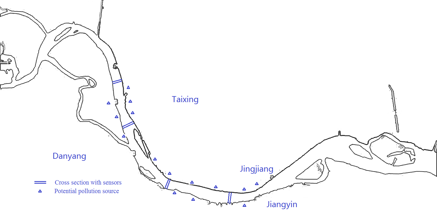
Figure 1: The river layout

2.3 Advection-Dispersion Equation

In this paper, the water pollutants are assumed to be released instantaneously from pollution sources. Once pollutants with the initial concentration $s$ are discharged in location $l$ and at time $t$, pollutants migrate and diffuse along the direction of water flow, and the pollutant concentration varies at different downstream cross sections considering the hydrodynamic characteristics. ADE (see Wang et al. (2018)) is commonly used to explain how the pollutants migrate and diffuse in the river. The analytical expression of ADE is defined as

$$C(l_{m},\,t_{m}^{n}|s,\,l,\,t):=\frac{s}{A\sqrt{4\pi D\left(t_{m}^{n}-t\right)}}\exp\left[-\frac{\left(l_{m}-l-v\left(t_{m}^{n}-t\right)\right)^{2}}{4D\left(t_{m}^{n}-t\right)}\right]\exp\left(-k\left(t_{m}^{n}-t\right)\right),$$ (1)

where $A$ is the water area perpendicular to the river flow direction ($\textrm{meter}^{2}$); $D$ is the dispersion coefficient in the flow direction, which is generally evaluated by empirical equations or based on experiments ($\textrm{meter}^{2}/\textrm{second}$); $v$ is the mean flow velocity of the cross section ($\textrm{meter}/\textrm{second}$); and $k$ is the decay coefficient ($\textrm{second}^{-1}$). In Equation (1), the term $l_{m}-l$ computes the length of $m$ cross section to the pollution source, along the river (geometrically, it is a curve).

In this case, our method is general and not limited to a one-dimensional problem. The physical meaning of Equation (1) is explained as follows: Given the known pollution source information $(s,\,l,\,t)$, the theoretical estimation of the concentration level monitored by sensor $m$ (at location $l_{m}$) at time $t_{m}^{n}$ equals $C(l_{m},\,t_{m}^{n}|s,\,l,\,t)$.

The “reverse” formulation of Equation (1) is denoted as $C(s,\,l,\,t|l_{m},\,t_{m}^{n})$, where the parameters and variables are exchanged. For this formulation, given sensor $m$ (at location $l_{m}$) at time $t_{m}^{n}$, the downstreaming concentration level can be predicted, given the estimated $(s,\,l,\,t)$.

2.4 Problem Formulation

As described in Section 2.2, the goal of the proposed method in this paper is to estimate the source information $(s,\,l,\,t)$, given the streaming concentration data collected by each sensor $c_{m}^{n}$. Equation (2) is then used to measure the gap between the theoretical estimation $C(s,\,l,\,t|l_{m},t_{m}^{n})$ value and the real data $c_{m}^{n}$:

$$\tilde{C}(s,\,l,\,t|l_{m},\,t_{m}^{n},\,c_{m}^{n}):= \frac{s}{A\sqrt{4\pi D\left(t_{m}^{n}-t\right)}}\exp\left[-\frac{\left(l_{m}-l-v\left(t_{m}^{n}-t\right)\right)^{2}}{4D\left(t_{m}^{n}-t\right)}\right]$$

$$\times\exp\left(-k\left(t_{m}^{n}-t\right)\right)-c_{m}^{n}.$$ (2)

For simplicity, use $\tilde{C}_{n,m}(s,\,l,\,t)$ to represent $\tilde{C}(s,\,l,\,t|l_{m},\,t_{m}^{n},\,c_{m}^{n})$ as defined by Eq. (2) throughout the paper. Instead of providing a theoretical estimation of the downstream concentration level, given the known information $(s,\,l,\,t)$, the ADE model is applied in a reverse-engineered manner, using $\tilde{C}_{n,m}(s,\,l,\,t)$ to indicate the estimation error of an estimated information $(s,\,l,\,t)$. Given any pollution source information estimation $(s,\,l,\,t)$, suppose $\tilde{C}_{n,m}(s,\,l,\,t)>0$. Then, the estimated concentration monitored by sensor $m$ at period $n$ is overestimated, and $\tilde{C}_{n,m}(s,\,l,\,t)<0$ means the estimated concentration is underestimated.

Given the estimated information $(s,\,l,\,t)$, the square function is used to quantify the estimation error of sensor $m$ at period $n$, denoted as $\left(\tilde{C}_{n,m}(s,\,l,\,t)\right)^{2}$. Namely, the estimation error of the $n$th period over sensor $m$ is defined as

$$\Psi(s,\,l,\,t|l_{m},\,t_{m}^{n},\,c_{m}^{n}) =\left(\tilde{C}_{n,m}(s,\,l,\,t)\right)^{2}.$$ (3)

Use $\Psi^{n}_{m}(s,l,t)$ to represent $\Psi(s,\,l,\,t|l_{m},\,t_{m}^{n},\,c_{m}^{n})$ for simplicity. The function $\Psi^{n}_{m}(s,\,l,\,t)$ on $(s,\,l,\,t)$ is called the loss function. In statistical learning, when the data $t^{n}_{m},\,c^{n}_{m}$ for all $n\in N$ are known in advance, the optimal source information can be identified by minimizing the average loss function $\sum_{n\in N}\Psi_{m}^{n}(s,\,l,\,t)$. In contrast, in online learning cases, the data $t^{n}_{m},\,c^{n}_{m}$ as well as the corresponding loss function $\Psi_{m}^{n}(s,\,l,\,t)$ are not completely known in advance but are sequentially accessible to the decision maker. Thus, regret the minimization method will be served as a new performance evaluation criterion other than the average loss minimization such that the estimation error of $(s,\,l,\,t)$ can be measured dynamically once the new sampling of concentration data is incorporated. In this paper, two “regret” definitions are presented, which measure the performance of online learning algorithms. They are called “cumulative regret” and “local regret.” In the well-established framework of OCO, numerous algorithms can efficiently achieve the optimal cumulative regret in the sense of converging in the total accumulated loss toward the best fixed decision in hindsight (see Hazan (2016) and Shalev-Shwartz (2012)). The “cumulative regret” is defined as follows.

Definition 2.1.

(Cumulative regret) Given an online learning algorithm $\mathcal{A}$, its cumulative regret with respect to sensor $m$ after $N$ iterations is denoted by

$$\mathfrak{R}_{m}^{\mathcal{A}}(N):=\sum_{n=1}^{N}\Psi^{n}_{m}(x^{n}_{m})-\inf_{x\in\mathcal{F}}\sum_{n=1}^{N}\Psi^{n}_{m}(x).$$ (4)

In the well-established framework of OCO, numerous algorithms can efficiently achieve optimal regret in the sense of converging in the average loss toward the best fixed decision in hindsight. That is, one can iterate $x_{m}^{1},\,...,\,x_{m}^{N}$ such that the long run average cumulative regret of $\mathcal{A}$,

$$\mathfrak{R}_{m}^{\mathcal{A}}(N)/N=\frac{1}{N}\sum_{n=1}^{N}\left[\Psi^{n}_{m}(x_{m}^{n})-\Psi^{n}_{m}(x)\right]=o(1).$$

However, even in the offline non-convex optimization case, it is too ambitious to converge toward a global minimizer in hindsight. The global convergence of offline non-convex optimization is normally NP-hard (see Hazan et al. (2017)). In the existing literature, it is common to state convergence guarantees toward an $\epsilon$-approximate stationary point; that is, there exists some iteration $x^{n}_{m}$ for which $\|\nabla\Psi^{n}_{m}(x^{n}_{m})\|\leq\epsilon$. Given the computational intractability of direct analogues of convex regret, the definition of “local regret” is given; it is a new notion of regret that quantifies the objective of predicting points with small gradients on average.

Throughout this paper, for convenience, the following notation from Hazan et al. (2017) is used to denote the sliding-window time average of functions, parameterized by some window size $1\leq w\leq N$:

$$F^{n}_{m,\,w}(x):=\frac{1}{w}\sum_{i=0}^{w-1}\Psi^{n-i}_{m}(x).$$

For simplicity, define $\Psi^{n}_{m}(x)$ to be identically zero for all $n\leq 0$.

Definition 2.2.

(Local regret) (Hazan et al., 2017, Definition 2.5) Fix some $\eta>0$. Define the $w$-local regret of an online algorithm with respect to sensor $m$ as

$$\mathfrak{R}_{m,w}(N):=\sum_{n=1}^{N}\left\|\nabla_{\mathcal{F},\eta}F^{n}_{m,w}(x^{n}_{m})\right\|^{2}.$$ (5)

In Hazan et al. (2017), the necessity of the time-smoothing term $w$ is argued such that for any online algorithm, an adversarial sequence of loss functions can force the local regret incurred to scale with $N$ as $\Omega(N/w^{2})$. This result indicates that “acceptable” online non-convex algorithms will only be able to achieve the linear local regret $O(N)$. In addition, the cumulative regret of online non-convex learning algorithms can be measured if the local properties on the local minimizer of $\Psi^{n}_{m}$ and $\sum_{n=1}^{N}\Psi^{n}_{m}$ are attained.

Furthermore, for some online learning problem where $F^{n}_{m,\,w}(x)\approx\Psi^{n}_{m}(x)$, a bound on the local regret truly captures a guarantee of playing points with small gradients. However, for any algorithm treating $F^{n}_{m,w}$ as the follow-the-leader objective when estimating $x^{n+1}_{m}$, the objective considers recording and summing up $w$ previous loss functions rather than all the historical loss functions up to iteration $n$. This setting saves the storage when the online algorithm is implemented.

2.5 Properties of Loss Functions

In this section, the mathematical properties of functions $\tilde{C}_{n,m}$ and $\Psi_{m}^{n}$ are figured, which underlines the development of the online algorithms. Throughout this paper, we denote the decision variables $x=(s,\,l,\,t)$ and $x^{\prime}=(s^{\prime},\,l^{\prime},\,t^{\prime})$ for simplicity. We use $\mathcal{S}$, $\mathcal{L}$ and $\mathcal{T}$ to denote the closed feasible set of $(s,\,l,\,t)$ and $\mathcal{F}:=\mathcal{S}\times\mathcal{L}\times\mathcal{T}$. The following assumptions on the set $\mathcal{F}$ are given first.

Assumption 2.3.

(i) $\mathcal{F}$ is a convex and compact set. (ii) For any $t\in\mathcal{T}$, $\min_{n\in N,m\in M}\left\{t_{m}^{n}\right\}>t$ holds. (iii) There exists $B>0$ such that $|\Psi_{m}^{n}(x)|\leq B$ for any $x\in\mathcal{F}$;

Assumption 2.3 (ii) indicates that any sensor monitors data collected after the pollution is discharged. Based on Assumption 2.3, the following Proposition 2.5 shows the “Lipschitz continuity” property of $\tilde{C}_{n,m}$ and its gradient on $\mathcal{F}$ by taking the first derivatives. Here, “Lipschitz continuity” is first defined in Definition 2.4 as follows.

Definition 2.4.

A function $f$ from $\mathcal{D}\subset\mathbb{R}^{d}$ to $\mathbb{R}$ is “Lipschitz continuous” at $x\in\mathcal{D}$ if there is a constant $K$ such that $|f(y)-f(x)|\leq K\|y-x\|$ for all $y\in\mathcal{D}$ sufficiently near $x$.

Proposition 2.5.

(i) $\tilde{C}_{n,m}$ is bounded and Lipschitz continuous on the set $\mathcal{F}$: Given any $x,\,x^{\prime}\in\mathcal{F}$, there exists $\sigma>0$ such that $\left|\tilde{C}_{n,m}(x)-\tilde{C}_{n,m}(x^{\prime})\right|\leq\sigma\|x-x^{\prime}\|$. (ii) The gradient of $\tilde{C}_{n,m}(x)$ is bounded and Lipschitz continuous on the set $\mathcal{F}$: Given any $x,\,x^{\prime}\in\mathcal{F}$, there exists $\gamma>0$ such that $\left\|\nabla_{x}\tilde{C}_{n,m}(x)-\nabla_{x}\tilde{C}_{n,m}(x^{\prime})\right\|\leq\gamma\|x-x^{\prime}\|$.

The following proposition shows the Lipschitz continuity properties of function $\Psi_{m}^{n}$.

Proposition 2.6.

(i) $\Psi_{m}^{n}$ is Lipschitz continuous on $\mathcal{F}$: Given any $x,\,x^{\prime}\in\mathcal{F}$, there exists $\kappa>0$ such that $\left\|\Psi_{m}^{n}(x)-\Psi_{m}^{n}(x^{\prime})\right\|\leq\kappa\|x-x^{\prime}\|$. (ii) $\Psi_{m}^{n}$ is $\beta$-smooth on $\mathcal{F}$: Given any $x,\,x^{\prime}\in\mathcal{F}$, there exists $\beta>0$ such that $\left\|\nabla_{x}\Psi_{m}^{n}(x)-\nabla_{x}\Psi_{m}^{n}(x^{\prime})\right\|\leq\beta\left\|x-x^{\prime}\right\|$. (iii) $\Psi_{m}^{n}$ is also $\iota$-Hessian Lipschitz: Given any $x,\,x^{\prime}\in\mathcal{F}$, there exists $\iota>0$ such that $\|\nabla_{(s,\,l,\,t)}^{2}\Psi_{m}^{n}(x)-\nabla_{(s,\,l,\,t)}^{2}\Psi_{m}^{n}(x^{\prime})\|\leq\iota\left\|x-x^{\prime}\right\|$.

Next, the definition of “projected gradient” is provided, and its properties are derived. These properties will be useful in designing and analyzing our online algorithms. The properties are naturally extended from Hazan et al. (2017), where the step size $\eta$ is univariate rather than a vector, as in our case.

Definition 2.7.

(Projected gradient) Let $\Psi_{m}^{n}:\,\mathcal{F}\rightarrow\mathbb{R}$ be a differentiable function on the compact and convex set $\mathcal{F}$. Let vector-valued step size be $\eta\in\mathbb{R}_{+}^{d}$ (throughout the paper, $d=3$ for pollution source identification problems), and we define $\nabla_{\mathcal{F},\eta}\Psi_{m}^{n}:\,\mathcal{F}\rightarrow\mathbb{R}^{d}$, the $(\mathcal{F},\,\eta)$-projected gradient of $\Psi_{m}^{n}$ by $\nabla_{\mathcal{F},\eta}\Psi_{m}^{n}(x):=\left(x-\Pi_{\mathcal{F}}\left[x-\eta\otimes\nabla_{x}\Psi_{m}^{n}(x)\right]\right)\oslash\eta$, where $\Pi_{\mathcal{F}}[\cdot]$ denotes the orthogonal projection onto $\mathcal{F}$, the symbol $\otimes$ denotes the Hadamard product, and $\oslash$ denotes the element-wise division of two vectors.

The following proposition shows that there always exists a point with a vanishing projected gradient.

Proposition 2.8.

Let $\mathcal{F}$ be a compact and convex set and suppose $\Psi_{m}^{n}:\mathcal{F}\rightarrow\mathbb{R}$ satisfies the properties in Proposition 2.6. Then, there exists some point $x^{\ast}\in\mathcal{F}$ for which $\nabla_{\mathcal{F},\eta}\Psi_{m}^{n}(x^{\ast})=0$.

The following proposition states that an approximate local minimum, as measured by a small projected gradient, is robust with respect to small perturbations. This proposition will be applied to derive the local regret bound of our proposed algorithms in Section 3.

Proposition 2.9.

Let $x$ be any point in $\mathcal{F},$ and let $\Psi$ and $\Phi$ be differentiable functions $\mathcal{F}\rightarrow\mathbb{R}$. Then, for any $\eta\in\mathbb{R}_{+}^{d}$ and $x\in\mathcal{F}$, $\left\|\nabla_{\mathcal{F},\,\eta}[\Psi+\Phi](x)\right\|\leq\left\|\nabla_{\mathcal{F},\,\eta}\Psi(x)\right\|+\left\|\nabla\Phi(x)\right\|$.

Note that the proofs of Proposition 2.5, 2.6, 2.8, and 2.9 are all provided in Appendix B.

3 The Algorithm

In this section, our basic algorithm (Algorithm 1), adaptive time-smoothed online gradient descent (ATGD), is developed. The key idea of this algorithm is to implement follow-the-leader iterations approximated to a suitable tolerance using projected gradient descent. Apart from the standard gradient descent paradigm, the improvements of our algorithm are: (i) adjusting the step sizes to be vectors, meaning that the algorithm performs different step sizes on different dimensions (released mass, location and released time). This setting avoids potentially slow updates on some dimensions and divergence on other dimensions, owing to the different magnitude of the gradient on different dimensions (i.e., a steep surface will have high gradient magnitude, and a flat surface will have low gradient magnitude). The vectorized step-size setting thus improves the robustness of the algorithm more than the univariant step-size version; (ii) the step-size is improved by line search and leads to faster convergence near the stationary points.

In Algorithm 1, $\mathfrak{S}(F^{n}_{m,w},\,K)$ is an operator choosing the initial step sizes, whose explicit definition will be given later. The explicit description of the normalized Backtracking-Armijo line search is shown in Algorithm 2, where a properly chosen $\beta$ prevents the step size from getting too large along the gradient descent direction, and the backtracking method prevents the step size from getting too small. Algorithm 2 is equipped with adaptive step sizes modified from the Backtracking-Armijo line search, which is one of the most widely investigated exact line search methods (see Dennis Jr and Schnabel (1996); Armijo (1966); Nocedal and Wright (2006)). Our new Armijo condition is imposed on the normalized gradient to further reduce the negative effect of a gradient magnitude difference on each dimension, in addition to the vector step-size setting. Term $\eta^{(l)}\beta\|\nabla_{\mathcal{F},\eta^{(l)}}F^{n}_{m,\,w}(x_{m}^{n+1})\|_{2}$, at the right side of the Armijo inequality, will approach zero when the norm of the projected gradient approaches zero, and then the condition will become the standard Backtracking line search. This setting leads to faster convergence near the stationary points. The following theorem indicates that Algorithm 2 terminates in a finite number of iterations. Its proof is given in Appendix C.

Theorem 3.1.

Algorithm 2 terminates in a finite number of iterations.

Algorithm 1 ATGD

Input: sensor $m\in M$; window size $w\geq 1$, tolerance $\delta>0$, constant $K>0$, and a convex set $\mathcal{F}$;

Set $x^{1}_{m}\in\mathcal{F}$ arbitrarily

for $n=1,\,...,\,N$ do

   Observe the cost function $\Psi^{n}_{m}:\,\mathcal{F}\rightarrow\mathbb{R}$.

   Compute the initial step-size: $\eta^{0}=\mathfrak{S}(F^{n}_{m,w},\,K)$.

   Initialize $x^{n+1}_{m}:=x^{n}_{m}$ and $\eta^{n}:=\eta^{0}$.

       while $\|\nabla_{\mathcal{F},\eta^{n}}F^{n}_{m,\,w}(x^{n+1}_{m})\|_{2}>\delta$ do

         Determine $\eta^{n}$ using Normalized Backtracking-Armijo line search (Algorithm 2).

         Update $x^{n+1}_{m}:=x^{n+1}_{m}-\eta^{n}\otimes\nabla_{\mathcal{F},\eta^{n}}F^{n}_{m,\,w}(x^{n+1}_{m})$.

      end while

end for

Algorithm 2 Normalized Backtracking-Armijo line search

Input: $\eta^{0}>0$, $x^{n+1}_{m}$ and $F^{n}_{m,\,w}$, let $\eta^{(0)}=\eta^{0}$ and $l=0$.

while $F^{n}_{m,\,w}(x^{n+1}_{m}-\eta^{(l)}\otimes\nabla_{\mathcal{F},\eta^{(l)}}F^{n}_{m,\,w}(x^{n+1}_{m})/\|\nabla_{\mathcal{F},\eta^{(l)}}F^{n}_{m,\,w}(x^{n+1}_{m})\|_{2})>F^{n}_{m,\,w}(x^{n+1}_{m})+\beta\|\eta^{(l)}\otimes\nabla_{\mathcal{F},\eta^{(l)}}F^{n,\,w}_{m}(x^{n+1}_{m})\|_{2}$ do

   Set $\eta^{(l+1)}=\tau\otimes\eta^{(l)}$, where $\tau\in(0,\,1)^{d}$ is fixed (e.g., $\tau=(1/2,\,1/2,\,1/2)$),

   Set $l=l+1$

end while

Set $\eta^{n}=\eta^{(l)}$

In terms of how proper initial step sizes can be chosen, the main idea is to set the initial step sizes on each dimension inversely proportional to the Lipschitz modulus of the loss on that dimension such that the algorithm can adjust the identification change on each dimension to a similar magnitude. A simple partition method is first derived to derive a lower bound on the Lipschitz modulus on each dimension from Gimbutas and Žilinskas (2016); Sergeyev et al. (2013); Pintér (2013). The initial step-size selection is presented by Algorithm 3. For simplicity, use the operator $\mathfrak{S}$ to encode the process of finding an initial step size in Algorithm 3. Given the function $F^{n}_{m,w}$ and constant $K>0$, the initial step size is $\eta^{0}=\mathfrak{S}(F^{n}_{m,w},\,K)$.

Algorithm 3 Initial step-sizes construction

Input: Function $F^{n}_{m,\,w}$ and $K>0$. Let $\eta^{0}\in\mathbb{R}^{d}_{+}$ denote initial step sizes at iteration $n$ with the step sizes on each dimension as $\eta_{s}^{0}$, $\eta_{l}^{0}$ and $\eta_{t}^{0}$.

    Generate $K^{3}$ points on cube $\mathcal{F}$, denoted as $(s^{1},...,\,s^{K})$, $(l^{1},...,\,l^{K})$ and $(t^{1},...,\,t^{K})$. In each dimension, the points are uniformly spaced in cube $\mathcal{F}$.

    Compute

$$\kappa^{n}_{s}=\max_{i,j,k,p=1,...,K}\left\{\frac{|F^{n}_{m,w}(s^{i},\,l^{k},t^{p})-F^{n}_{m,w}(s^{j},\,l^{k},t^{p})|}{|s^{i}-s^{j}|}:\,i\neq j\right\},$$

$$\kappa^{n}_{l}=\max_{i,j,k,p=1,...,K}\left\{\frac{|F^{n}_{m,w}(s^{k},\,l^{i},t^{p})-F^{n}_{m,w}(s^{k},\,l^{j},t^{p})|}{|l^{i}-l^{j}|}:\,i\neq j\right\},$$

and

$$\kappa^{n}_{t}=\max_{i,j,k,p=1,...,K}\left\{\frac{|F^{n}_{m,w}(s^{k},\,l^{p},t^{i})-F^{n}_{m,w}(s^{k},\,l^{p},t^{j})|}{|t^{i}-t^{j}|}:\,i\neq j\right\},$$

to be the Lipschitz modulus estimation on dimension $s$, $l$, and $t$ respectively.

    Update $\eta^{0}$ such that it satisfies the following two conditions: (i) for the validation and analysis of the algorithm, choose a sufficiently large initial step size such that $\|\eta^{0}\|_{\min}/\|\eta^{0}\|_{\infty}^{2}\gg\beta/2$, and (ii) the equations $\eta^{0}_{s}/\kappa^{n}_{s}=\eta^{0}_{l}/\kappa^{n}_{l}=\eta^{0}_{t}/\kappa^{n}_{t}$ hold.

3.1 Performance Analysis

In this subsection, the analysis of the regret bound (i.e., the upper bound on the local regret) for Algorithm 1 is shown in addition to the derivation of the optimal window size to minimize the regret bound within a limited number of gradient estimations.

The following Theorem 3.2 presents the local regret and the total number of required gradient estimations. The proof of Theorem 3.2 is given in Appendix C.

Theorem 3.2.

Let $N$ denote the number of samplings. Given sensor $m\in M$, let $\Psi^{1}_{m},\,...,\,\Psi^{N}_{m}$ be the sequence of loss functions presented to Algorithm 1, satisfying the properties in Proposition 2.6. Then,

(i) The $w$-local regret incurred satisfies

$$\mathfrak{R}_{m,w}(N)\leq(\delta+\frac{2\kappa}{w})^{2}N.$$ (6)

(ii) There exists $\eta^{\prime}\leq\eta^{0}$ such that the total number of gradient steps taken by Algorithm 1 is bounded by

$$\frac{2B}{\delta^{2}\left(\|\eta^{\prime}\|_{\min}-\frac{\beta\,\|\eta_{0}\|_{\infty}^{2}}{2}\right)w}N,$$ (7)

where $B$ is the bound of the loss function stated in Assumption 2.3.

Theorem 3.2 illustrates that Algorithm 1 attains the local regret bound $O(N/w^{2}+N/w+N)$ with $O(N/w)$ gradient evaluation steps. Theorem 3.2 (i) illustrates that ATGD has the average local regret $\mathfrak{R}_{w}(N)/N=O(1)$. Such performance is thus acceptable, as mentioned previously in Section 2.4. Besides, the bound (7) is larger than the bound in (Hazan et al., 2017, Algorithm 1) owing to the diminishing step sizes, which will lead to more gradient estimations of Algorithm 1 than (Hazan et al., 2017, Algorithm 1) but will lead to a lower local regret bound than (Hazan et al., 2017, Algorithm 1) given the fixed number of gradient estimations. The results reveal a tradeoff between low computational complexity and high convergence guarantee. Moreover, our results show that for a fixed streaming data size $N$, increasing the window size $w$, that is, increasing the smoothing effect, will reduce both the complexity of the local regret and the total number of gradient steps. In terms of the lower bound on local regret, it is shown from (Hazan et al., 2017, Theorem 2.7) that for any online algorithm, an adversarial sequence of loss functions can force the local regret incurred to scale with $N$ as $\Omega(N/w^{2})$.

The optimal window size $w^{\ast}$ can be determined when fixing computational resources (i.e., fixing the number of gradient estimations) such that the local regret bound can be minimized. By fixing the bound on the total number of gradient steps as $T$, the required size of input data will be

$$N=\frac{\delta^{2}\left(\|\eta^{\prime}\|_{\min}-\frac{\beta\,\|\eta^{0}\|_{\infty}^{2}}{2}\right)w}{2B}T.$$

The bound on the $w$-local regret will become

$$\left[\delta^{2}w+4\delta\kappa+\frac{4\kappa^{2}}{w}\right]\frac{\delta^{2}\left(\|\eta^{\prime}\|_{\min}-\frac{\beta\,\|\eta^{0}\|_{\infty}^{2}}{2}\right)}{2B}T.$$

By minimizing the $w$-local regret in $w$, the optimal window size $w^{\ast}$ will equal $1$ if $2\kappa/\delta\leq 1$ and $N$ if $2\kappa/\delta\geq N$. When $1<2\kappa/\delta<N$, the optimal window size $w^{\ast}$ will equal $2\kappa/\delta$. Thus, the optimal window size $w^{\ast}$ is dependent on the Lipschitz-continuous modulus of function $\Psi_{n}$ as well as the tolerance level $\delta$, but is independent on the gradient step sizes as well as the computational budget. To interpret this, the more “fluctuation” the shape of loss functions has and the more accurate the estimation requirement on the algorithm is, the larger the required window sizes that should be chosen. In another words, the optimal window size should be determined based on the specific properties of the pollution source (choice of ADE model) and the parameters of the river (choice of ADE model parameters).

Remark 3.3.

(i) Suppose the step sizes are constant in Algorithm 1, where step sizes $\{\eta^{n}\}$ are replaced with $\eta^{0}$ and the Backtracking-Armijo line-search step will not be implemented. Then, Theorem 3.2 will still hold for the new algorithm by replacing $\eta^{\prime}$ with $\eta^{0}$ in the bound (7). When $\{\eta^{n}\}$ becomes a constant and uni-variant value, Algorithm 1 will become (Hazan et al., 2017, Algorithm 1). Thus, our Algorithm 1 generalizes (Hazan et al., 2017, Algorithm 1).

(ii) From the proof of Theorem 3.2 in Appendix C, the theoretical guarantee of Algorithm 1 summarized in the theorem is independent of the structure of the inner loop updating the step sizes. In other words, Algorithm 2 can be replaced with other adaptive step-size approaches (e.g., the Backtracking-Armijo line search, Generic line search, and Exact line search) only if those methods continue to reduce the step sizes when the stopping criterion is not satisfied. Thus, an analytic framework for gradient-based online non-convex optimization algorithms is developed with adjusted step sizes by the line search.

3.2 Sequential Sensor Installation Mechanism

In this section, a case where a measurement error exists in the computed identification results in each iteration $n\in[N]$ is considered. In real life, the error can consist of systematic error from the measurements of sensors and random error from the experimenter’s interpretation of the instrumental reading and unpredictable environmental condition fluctuations. Normal (Gaussian) distribution is the most commonly used distribution for the measurement error, both in theory and practice (see Chesher (1991); Fuller (1995); Kelly (2007); Ruotsalainen et al. (2018); Coskun and Oosterhuis (2020)). Assume the measurement error follows multivariate normal distribution among sensors in each iteration $n\in[N]$, and the distribution is stationary for all $n\in[N]$. However, the explicit distribution and its mean and variance are not known. Installing multiple sensors can help reduce the measurement error, but implementing such sensors is an extremely costly activity, including costs for manpower, equipment, and chemical reagents (see Chinrungrueng et al. (2006); Carlsen et al. (2008); Park et al. (2012); Abubakar et al. (2015); Dong et al. (2017)). Thus, there is a trade-off between the costs and measurement accuracy requirements. The goal of the section is to find the minimal number of sensors possible such that the measurement error can be controlled.

The confidence interval for the source identification result is first derived when $|M|$ is given. As the normal distribution is assumed, and standard deviation is unknown, the confidence interval is constructed based on the Student’s $t$-distribution theory. Denote $x^{n}_{m}=(s^{n}_{m},\,l^{n}_{m},\,t^{n}_{m})$ as the identification results output from Algorithm 1 at sensor $m\in M$ using the first $n$th iterations. The mean across all sensors can be computed as

$$\bar{x}^{n}=(\bar{s}^{n},\,\bar{l}^{n},\,\bar{t}^{n})=\frac{1}{|M|}\sum_{m\in M}x^{n}_{m}=(\frac{1}{|M|}\sum_{m\in M}s^{n}_{m},\,\frac{1}{|M|}\sum_{m\in M}l^{n}_{m},\,\frac{1}{|M|}\sum_{m\in M}t^{n}_{m}).$$

The standard deviation on each dimension is $S_{s^{n}}=\sqrt{\frac{1}{|M|-1}\sum_{m\in M}(s^{n}_{m}-\bar{s}^{n})^{2}}$, $S_{l^{n}}=\sqrt{\frac{1}{|M|-1}\sum_{m\in M}(l^{n}_{m}-\bar{l}^{n})^{2}}$ and $S_{t^{n}}=\sqrt{\frac{1}{|M|-1}\sum_{m\in M}(t^{n}_{m}-\bar{t}^{n})^{2}}$, respectively. The next proposition derives the confidence interval for the released mass identification result as an example. The confidence intervals for the location and time identification results can be derived using the same idea.

Proposition 3.4.

(Sutradhar (1986); Taboga (2017); Prins (2013)) Given the set of sensors $M$, the $(1-\alpha)$ confidence interval for the released mass identification result after $n$ iterations is

$$\left[\bar{s}^{n}-t_{\alpha/2,\,|M|-1}\frac{S_{s^{n}}}{\sqrt{|M|}},\,\bar{s}^{n}+t_{\alpha/2,\,|M|-1}\frac{S_{s^{n}}}{\sqrt{|M|}}\right],$$ (8)

where $t_{\alpha/2,\,|M|-1}$ is the two-sided $t$-value for $1-\alpha$ confidence under $|M|-1$ degree of freedom. This value can be found from the standard table in (Prins, 2013, Chapter 1.3.6.7.2.).

Suppose $d^{s},\,d^{l}$ and $\,d^{t}$ are the acceptable length of confidence intervals, under $1-\alpha$ confidence on each dimension, respectively, set by the decision maker. These also quantify the estimation accuracy requirement. Given formulation Equation (8), a natural idea to compute the minimal sensors required on each dimension is to set $d^{s},\,d^{l},\,d^{t}$ equal to the lengths of the corresponding confidence intervals. For instance, $d^{s}=2t_{\alpha/2,\,|M|-1}\frac{S_{s^{n}}}{\sqrt{|M|}}$. The $|M|$ satisfying the equation is the minimal number of sensors required to ensure estimation accuracy at the concentration level. The drawback is that the two-sided $t$-value depends on known degrees of freedom, which in turn depends upon the sample size that we are trying to estimate. To solve this problem, a power analysis procedure is proposed, starting with an initial estimate based on a sample standard deviation and iteration (see (Prins, 2013, Section 7.2.2.2.)). However, this power analysis still has a drawback in real life applications because it may output a required number of sensors that is more than the number of sensors that exist in reality, and these extra samples cannot be collected.

A sequential method is proposed, as summarized in Algorithm 4. In the algorithm, first, Partition $N$ iterates with several rounds, and each contains the $T$ iteration. The total rounds are $\lfloor N/T\rfloor+1$. The number of iterations in the final rounds is the remainder. Suppose $A$ sensors are installed initially; that is, $|M_{0}|=A>0$ (e.g., $A=2$). Then, at each round $i=1,...,\lfloor N/T\rfloor+1$, only the data within that round are used for identification (the identification results in previous rounds will be deleted, and the online learning algorithms will again have a cold start). Choose the data from $n\in\{2,...,|M_{i-1}|\}$ sensors. If the updated required sensor number $|\tilde{M_{i}^{s}}|$ is larger than the current one $|M_{i-1}|$, then the algorithm will jump out of the current round, and the extra sensors will be installed up to $|\tilde{M_{i}^{s}}|$. Otherwise, a new $|\tilde{M_{i}^{s}}|$ will be updated by the bisection method. The required number of sensors for the released mass $s$ is the minimal value $|\tilde{M_{i}^{s}}|$ across all $n\in\{2,...,|M_{i-1}|\}$. The same procedures will be applied to estimate the location ($l$) and time ($t$). Then, the required number of sensors used for the next round $i+1$ will be the maximum across all dimensions.

Algorithm 4 Sequential Sensor Installation Design

Input: Partition $N$ iterations with several rounds, and each contains $T$ iteration. The total number of rounds is $\lfloor N/T\rfloor+1$. The number of iterations in the final rounds is the remainder. Initialize $|M_{0}|=A>0$;

for $i=1,...,\lfloor N/T\rfloor+1$ do

   Denote the initial required sensor size for the concentration level at round $i$ to be $|M_{i-1}|$.

   for $n=2,...,|M_{i-1}|$ do

      Set $|M_{i}^{s}|=n$. Arbitrarily set $\hat{|M_{i}^{s}|}\neq|M_{i}^{s}|$.

      while $\hat{|M_{i}^{s}|}\neq|M_{i}^{s}|$, do

         Compute $\bar{s}^{T}=\frac{1}{|M_{i}^{s}|}\sum_{m\in M_{i}^{s}}s^{T}_{m}$ where $s^{T}_{m}$ is the identification results at the end of iteration $T$, only using the data in round $i$.

         Compute $S_{s^{T}}=\sqrt{\frac{1}{|M_{i}^{s}|-1}\sum_{m\in M_{i}^{s}}(s^{T}_{m}-\bar{s}^{T})^{2}}$.

         Update $\hat{|M_{i}^{s}|}=\lceil\left(t_{\alpha/2,\,|M_{i}^{s}|-1}\leavevmode\nobreak\ S_{s^{T}}/d^{s}\right)^{2}\rceil$.

         Update $|\tilde{M_{i}^{s}}|=\lceil\left(|M_{i}^{s}|+\hat{|M_{i}^{s}|}\right)/2\rceil$.

         if $|M_{i-1}|<|\tilde{M_{i}^{s}}|$, then

            break

         Set $|M_{i}^{s}|=\tilde{|M_{i}^{s}|}$.

      end while

      Set $R^{s}_{i,n}=\tilde{|M_{i}^{s}|}$, where $R^{s}_{i,n}$ records the number of sensors w.r.t to concentration $s$.

   end for

   Using the similar procedures (in the above for loop) w.r.t location $l$ and time $t$. Set

$$|M_{i}|=\max\{\min_{n}\{R^{s}_{i,n}\},\,\min_{n}\{R^{l}_{i,n}\},\,\min_{n}\{R^{t}_{i,n}\}\}.$$

end for

4 Escaping from Saddle Points

In this section, the basic algorithm (Algorithm 1) is further extended in terms of its practical implementation by deriving the module “escaping from saddle points”, which helps the algorithm arrive at a local minima with a high probability instead of being stuck in any first-order stationary point. We also show the cumulative regret of the algorithm under an error bound condition on the loss functions.

In non-convex optimization, the convergence to first-order stationary points (points where first-order derivatives equal zero) is not satisfactory. For non-convex functions, first-order stationary points can be global minima, local minima, saddle points, or even local maxima. For many non-convex problems, it is sufficient to find a local minimum. In each iteration ($n$) in our basic algorithm ATGD, the algorithm will terminate when $x^{n}_{m}$ is the $\delta$-first-order stationary point of the follow-the-leader iteration $F^{n}_{m,w}$ on $\mathcal{F}$. However, such a point may not necessarily be the local minimum of $\Psi^{n}_{m}$. Additional techniques are required to escape all saddle points and arrive at the local minima.

Based on Proposition 2.6(iii) and triangle inequality, it can be shown that $\nabla_{x}^{2}F^{n}_{m,w}(x)$ is also $\iota$-Hessian Lipschitz. The definitions of the second-order stationary point and $\epsilon$-second-order stationary point are given.

Definition 4.1.

Nesterov and Polyak (2006); Jin et al. (2017) For the $\iota$-Hessian Lipschitz function $F^{n}_{m,w}$, the point $x$ is a second-order stationary point if $\|\nabla_{x}F^{n}_{m,w}(x)\|=0$ and $\lambda_{\min}\left(\nabla_{x}^{2}F^{n}_{m,w}(x)\right)\geq 0$. The point $x$ is a $\epsilon$-second-order stationary point if

$$\|\nabla_{x}F^{n}_{m,w}(x)\|\leq\epsilon,\quad\textrm{and}\quad\lambda_{\min}\left(\nabla_{x}^{2}F^{n}_{m,w}(x)\right)\geq-\sqrt{\iota\,\epsilon}.$$

Second-order stationary points are important in non-convex optimization because when all saddle points are strict ($\lambda_{\min}\left(\nabla_{x}^{2}F^{n}_{m,w}(x)\right)<0$), all second-order stationary points are exactly the local minima. The goal here is to design algorithms that converge to the $\epsilon$-second-order stationary point, provided the threshold $\epsilon>0$.

A robust version of the “strict saddle” condition is next provided and holds for function $F^{n}_{m,w}$ based on Ge et al. (2015); Jin et al. (2017).

Proposition 4.2.

Function $F^{n}_{m,w}(\cdot)$ is $(\theta,\,\tau,\,\zeta)$-strict saddle with $\theta,\,\tau>0$ and $\zeta\geq 0$. That is, for any $x$, at least one of the following holds: (i) $\|\nabla_{x}F^{n}_{m,w}(x)\|\geq\theta$; (ii) $\lambda_{\min}\left(\nabla_{x}^{2}F^{n}_{m,w}(x)\right)\leq-\tau$; (iii) $x$ is $\zeta$-close to the set of the local minima of $F^{n}_{m,w}$.

Algorithm 5 is a perturbed form of the gradient descent algorithm. For each iteration $n$ in Algorithm 5, the algorithm will search for the solution where the current gradient is small ($\leq\delta$) (which indicates that the current iteration $x_{t}^{n}$ is potentially near a saddle point), the algorithm adds a small random perturbation to the gradient. The perturbation is added at most only once every $t_{\textrm{thres}}$ iterations. If the function value does not decrease enough (by $f_{\textrm{thres}}$) after $t_{\textrm{thres}}$ iterations, the algorithm will output $\tilde{x}^{n+1,t_{\textrm{noise}}}$. This can be proven to be necessarily close to a local minima. The step-size choice operator $\mathfrak{S}(F^{n}_{m,w},\,K)$, instead of requiring the condition $\|\eta^{0}\|_{\min}/\|\eta^{0}\|_{\infty}^{2}\gg\beta/2$ in Algorithm 1, requires $\|\eta^{0}\|_{\infty}=c/\kappa$ in Algorithm 5.

Algorithm 5 Adaptive perturbed time-smoothed online gradient descent (APTGD)

Input: sensor $m\in M$, window size $w\geq 1$, Constant $c\leq 1$, tolerance $\delta>0$, contant $K>0$, and a convex set $\mathcal{F}$;

Input: $\mathcal{\chi}=3\max\left\{\log\left(\frac{d\kappa\triangle f}{c\delta^{2}\epsilon}\right),\,4\right\}$, $r=\frac{\sqrt{c}}{\chi^{2}}\cdot\frac{\delta}{\kappa}$, $g_{\textrm{thres}}=\frac{\sqrt{c}}{\mathcal{\chi}^{2}}\cdot\delta$, $f_{\textrm{thres}}=\frac{c}{\mathcal{\chi}^{3}}\sqrt{\frac{\delta^{3}}{\iota}}$, $t_{\textrm{thres}}=\lceil\frac{\chi}{c^{2}}\cdot\frac{\kappa}{\sqrt{\iota\,\delta}}\rceil$, $t_{\textrm{noise}}=-t_{\textrm{thres}}-1$

Set $x^{1}_{m}\in\mathcal{F}$ arbitrarily.

for $n=1,\,...,\,N$ do

   Observe the cost function $\Psi^{n}_{m}:\,\mathcal{F}\rightarrow\mathbb{R}$.

   Compute the initial step size: $\eta^{0}=\mathfrak{S}(F^{n}_{m,w},\,K)$.

   Initialize $x^{n+1}_{m}:=x^{n}_{m}$ and $t_{\textrm{noise}}$;

   for $t=0,\,1,\,...$ do

      Initialize $x^{n+1,t}:=x^{n+1}_{m}$;

      Determine $\eta^{t}$ using Normalized Backtracking-Armijo line search (Algorithm 2).

       if $\|\nabla_{\mathcal{F},\eta^{t}}F^{n}_{m,\,w}(x^{n+1,t})\|\leq g_{\textrm{thres}}$ and $t-t_{\textrm{noise}}>t_{\textrm{thres}}$ then

         $t_{\textrm{noise}}=t$, $\tilde{x}^{n+1,t}=x^{n+1,t}$, $x^{n+1,t}=\tilde{x}^{n+1,t}+\omega$ where $\omega$ uniformly sampled from $\mathbb{B}_{0}(r)$

       if $t-t_{\textrm{noise}}=t_{\textrm{thres}}$ and $F_{n,\,w}(x^{n+1,t})-F_{n,\,w}(\tilde{x}^{n+1,t_{\textrm{noise}}})>-f_{\textrm{thres}}$ then

         Return $x^{n+1}_{m}=\tilde{x}^{n+1,t_{\textrm{noise}}}$

      Update $x^{n+1,t+1}=x^{n+1,t}-\eta^{t}\otimes\nabla_{\mathcal{F},\eta^{t}}F^{n}_{m,\,w}(x^{n+1,t})$.

   end for

end for

Theorem 4.3.

Let $\Psi^{n}_{m}$ satisfy properties in Proposition 2.6 and 4.2. There exists an absolute constant $c_{max}\leq 1$ such that for $c\leq c_{max}$, and $\triangle f\geq\max_{n=1,\,...,\,N}\left\{F^{n}_{m,w}(x^{n-1}_{m})\right\}$ by letting $\delta:=\min\left(\theta,\,\tau^{2}/\iota\right)$, Algorithm 5 will output a sequence of $\delta$-second-order stationary points that are also the $\zeta$-close local minima of $\{F^{n}_{m,\,w}\}_{n=1,\,...,\,N}$, with the probability $1-\epsilon$, and terminate in the following total number of iterations (gradient estimations):

$$O\left(\frac{\kappa\triangle f}{\delta^{2}}\log^{4}\left(\frac{d\kappa\triangle f}{\delta^{2}\,\epsilon}\right)N\right).$$ (9)

The proof of Theorem 4.3 is shown in Appendix D, which follows the results in Jin et al. (2017). Here, their results on the standard gradient descent can be naturally extended to the online gradient descent, as our basic algorithm contains an offline follow-the-leader oracle at each period. Theorem 4.3 shows that by careful selection of $\triangle f$ and $\delta$, the algorithm will output the local minima of each follow-the-leader oracle in each period with a linear number of iterations in a high probability. As mentioned in Jin et al. (2017), Theorem 4.3 only explicitly asserts that the output will lay within some fixed radius $\zeta$ from a local minimum. In many real applications, $\zeta$ can be further written as a function $\zeta(\cdot)$ of the gradient threshold $\theta$ such that $\theta$ decreases, $\zeta(\theta)$ decreases linearly or polynomially depending on $\theta$. The following Definition 4.4 is given, based on which Example 4.5 is given. Given the complexity of the objective $F^{n}_{m,w}$, the Example 4.5 ensures that $\zeta(\theta)$ decreases linearly on $\theta$ with a high probability.

Definition 4.4.

(Restricted strongly convex) (Zhang, 2017, Definition 1 and Definition 2) Let the nonempty set $\mathcal{X}\subset\mathcal{F}$ be the set of all local minimum of $F^{n}_{m,w}$. Then, function $F^{n}_{m,w}$ is restricted and strongly convex with the constant $\mu>0$ if it satisfies the restricted secant inequality

$$\langle\nabla_{x}F^{n}_{m,w}(x),\,x-\Pi_{\mathcal{X}}[x]\rangle\geq\mu\leavevmode\nobreak\ d^{2}(x,\,\mathcal{X}),$$

where $d(x,\,\mathcal{X})$ measures the distance from a point $x$ to set $\mathcal{X}$.

Example 4.5.

(Local error bound) Based on Luo and Tseng (1993); Drusvyatskiy and Lewis (2018), and assuming that restricted strongly convexity in Definition 4.4 holds when $x$ lays within the fixed radius $\zeta$ from a local minimum, the function $F^{n}_{m,w}$ is strongly convex in the $\zeta$-ball of any local minimum, and then the local error bound condition holds that

$$d(x,\,\mathcal{X})\leq\mu\|\nabla_{x}F^{n}_{m,w}(x)\|,$$

for all $n=1,...,N$. Thus, in this example, $\zeta$ decreases linearly on $\theta$ with the rate $\mu>0$; that is, $\zeta(\theta)=\mu\theta$. Suppose Algorithm 5 outputs the solution $x_{m}^{n}$ at each iteration $n$. Luo and Tseng (1993) finds that if $F^{n}_{m,w}$ is strongly convex on $\mathcal{F}$, then the local error bound condition holds for all $x\in\mathcal{F}$. The following steps provide a valid way of checking if the result holds with a high probability, and the main idea is to check the strong convexity of $F^{n}_{m,w}$ on the $\zeta$-domain of $x_{m}^{n}$:

Step 1. Compute the Hessian $\nabla_{x}^{2}F^{n}_{m,w}(x_{m}^{n})$ and estimate $\mu$ such that $\mu$ is a lower bound for the smallest eigenvalue of the Hessian.

Step 2. Simulate a set of points in the $\mu\theta$-domain of $x_{m}^{n}$ and check if the Hessian of $F^{n}_{m,w}$ at those points are positive definite. If so, then the local error bound holds for function $F^{n}_{m,w}$ with a high probability.

For the above Step 2, instead of checking the positive definiteness of all the points in the $\mu\theta$-domain of $x_{m}^{n}$, finite points are generated and checked (see (Milne, 2018, Theorem 3)) such that the local error bound condition holds with a high probability.

Next, it can be shown that the local regret can be linked with the cumulative regret of Algorithm 5 under specific error bound conditions. The local error bound condition on function $\{\Psi^{n}_{m}\}_{n=1,...,N}$ is required, as summarized by the following assumption, where $w=1$.

Assumption 4.6.

Let $x^{n,\ast}_{m}$ be any local minimum of the function $\Psi^{n}_{m}$; then,

$$\|\nabla_{x}F^{n}_{m,\,1}(x)\|=\|\nabla_{x}\Psi^{n}_{m}(x)\|\geq\frac{\mu}{\kappa}\left[\Psi^{n}_{m}(x)-\Psi^{n}_{m}(x_{m}^{n,\ast})\right],$$

when $x$ lays within the fixed radius $\zeta$ from $x_{m}^{n,\ast}$. There also exists $x^{n,\ast}_{m}$ such that $x^{n}_{m}$ satisfies the condition.

To check if $\Psi^{n}_{m}$ satisfies Assumption 4.6, the following steps are required, which follow the similar idea in Example 4.5. Owing to the complexity of the objective $\Psi^{n}_{m}$, this method only ensures that Assumption 4.6 holds with a high probability:

Step 1. Solve the local minimum of $\Psi^{n}_{m}(x)$ denoted by $x^{n,\prime}_{m}$ by Algorithm 5.

Step 2. Compute the Hessian $\nabla_{x}^{2}\Psi^{n}_{m}(x^{n,\prime}_{m})$ and estimate $\mu$ such that $\mu/\kappa$ is a lower bound for the smallest eigenvalue of the Hessian.

Step 3. Simulate a set of points in the $\mu\theta$-domain of $x_{m}^{n,\prime}$ and check if the Hessian of $\Psi^{n}_{m}$ at those points are positive definite. Then, check if $x^{n}_{m}$ lays within the $(\mu\theta)/\kappa$-domain of $x^{n,\prime}_{m}$.

The following Theorem 4.7 provides a high probability bound for the cumulative regret of Algorithm 5 with $O(N)$; the proof is given in Appendix D.

Theorem 4.7.

Let $\Psi_{m}^{n}$ satisfy Assumption 4.6. Then, with probability is at most $1-\epsilon$, and the cumulative regret of Algorithm 5 after

$$O\left(\frac{\kappa\triangle f}{\delta^{2}}\log^{4}\left(\frac{d\kappa\triangle f}{\delta^{2}\,\epsilon}\right)\cdot N\right)$$

gradient estimations, with $\triangle f\geq\max_{n=1,\,...,\,N}\left\{F^{n}_{m,w}(x^{n-1}_{m})\right\}$ and $\delta:=\min\left(\theta,\,\tau^{2}/\iota\right)$, is bounded by

$$O\left(\frac{\mu\delta}{\kappa}\cdot N\right).$$ (10)

Remark 4.8.

For practical implementation, the multi-start version algorithms can be developed for both ATGD and APTGD. The main idea is to create several solution paths when implementing the algorithms given different starting points. In each iteration, the square of the difference between the ADE value and real concentration data for each sensor is recorded. Following the idea from Jiang et al. (2015), the minimizer of the average of the square of the difference across all sensors, among all solution paths, is chosen, and we treat it as the estimated optimal solution at that iteration. Practically, the multi-start implementation can increase the chance of finding more accurate source information estimation. The explicit structures of multi-start algorithms are shown as Algorithm 7 (Multi-start time-smoothed online gradient descent, or MTGD) and Algorithm 8 (Multi-start perturbed time-smoothed online gradient descent, or MPTGD) in Appendix A.

5 Experiments and Application

In this section, the experiments validating the theoretical result of our online learning algorithms are conducted. Our algorithms are also applied to real-life river pollution source identification problems. For the experiments, the Rhodamine WT dye concentration data from a travel time study on the Truckee River between Glenshire Drive near Truckee, California and Mogul, Nevada (Crompton, 2008) are used. Figure 2 presents locations of a pollutant site, marked by a black star, and four sampling sites (sensors), marked by red stars. The data include the real data: the true pollutant source information $(s,\,l,\,t)=[1300,-22106,-215]$ and 82 pairs of concentration data detected in the four downstream sampling sites, and 1000 pairs of artificial data generated by the ADE model under the the true pollutant source information. The parameters in the ADE model are obtained from Crompton (2008) and Jiang et al. (2017); namely, $v=80m/min,D=2430m^{2}/min,A=60m^{2},$ and $k=10^{-8}min^{-1}$.

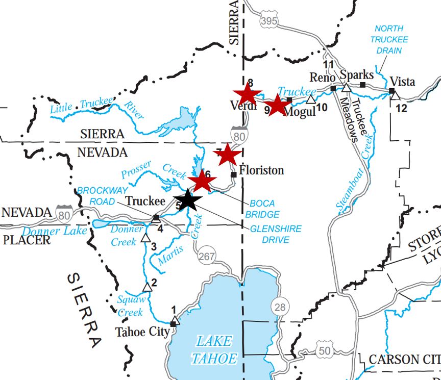
Figure 2: Locations of the pollutant site and sampling sites on the Truckee River

5.1 Regret and Optimality Analysis

In this experiment, 1000 pairs of artificially generated concentration data are used to compute the local regret bound (5) and the cumulative regret bound (4) for various online algorithms, including: time-smoothed online gradient descent (Hazan et al., 2017, Algorithm 1) (called “TGD” in short), ATGD, APTGD, MTGD, and MPTGD. TGD is explicitly presented as Algorithm 6. The step size is chosen to be $\eta=10$ throughout all the experiments in the following sections.

Algorithm 6 TGD

Input: Sensor $m\in M$; window size $w\geq 1$, learning rate $0<\eta\leq\beta/2$; tolerance $\delta>0$, constant $K>0$, and a convex set $\mathcal{F}$;

Set $x^{1}_{m}\in\mathcal{F}$ arbitrarily

for $n=1,\,...,\,N$ do

    Predict $x^{n}_{m}$. Observe the cost function $\Psi^{n}_{m}:\,\mathcal{F}\rightarrow\mathbb{R}$.

    Initialize $x^{n+1}_{m}:=x^{n}_{m}$.

       while $\|\nabla_{\mathcal{F},\eta}F^{n}_{m,\,w}(x^{n+1}_{m})\|_{2}>\delta/w$ do

          Update $x^{n+1}_{m}:=x^{n+1}_{m}-\eta\nabla_{\mathcal{F},\eta}F^{n}_{m,\,w}(x^{n+1}_{m})$.

      end while

end for

Choose the window size $w=1$. The group size (number of multi-starts) is chosen as $I=30$ in the multi-start algorithms. The initial step sizes are chosen by the method summarized in Section 3.1. The experimental results are recorded from Figure 3. Figure 3(a) validates that all of those algorithms have the local regret bound $O(N)$ as the inequality (6), and they also show experimentally that the cumulative regret of all those algorithm has the complexity $O(N)$, which potentially conforms to the bound (10). In addition, when all the algorithms are implemented, an extreme small tolerance $\delta=5\times 10^{-6}$ is set. Thus, in each iteration, the algorithms always stop close to a stationary point (can be either the saddle point or local minimum) for the current follow-the-leader iteration. So the local regrets of all the algorithms will be extremely low (within $2\times 10^{-5}$). Figure 3(a) shows that the vectorized and adaptive step-size algorithms slightly improve the accuracy of the stationary point search in each iteration compared to the fixed and univariate step-size algorithms. Particularly for MTGD and MPTGD, the local regret increases slightly as the number of iterations increases.

From the plots of cumulative regret, it can be observed that adding the “escaping from saddle points” module can reduce the growth rate of the cumulative regrets, which means that as the size of data grows, the algorithms output a solution closer to the global minimizer, that is, the true source information. Figure 3(b) shows that multi-start algorithms (MTGD and MPTGD) can further reduce the cumulative regrets. MPTGD has a significantly better cumulative regret than all other algorithms. Intuitively, the potential reason is the aggregated effect of the “perturbed” module and the multi-start module. The “perturbed” module increases the probability of convergence to a local minimum. The multi-start module ensures that the probability that the global minimum is among the multiple local minimums will be high.

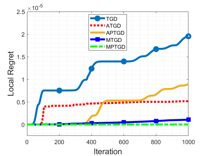
(a)

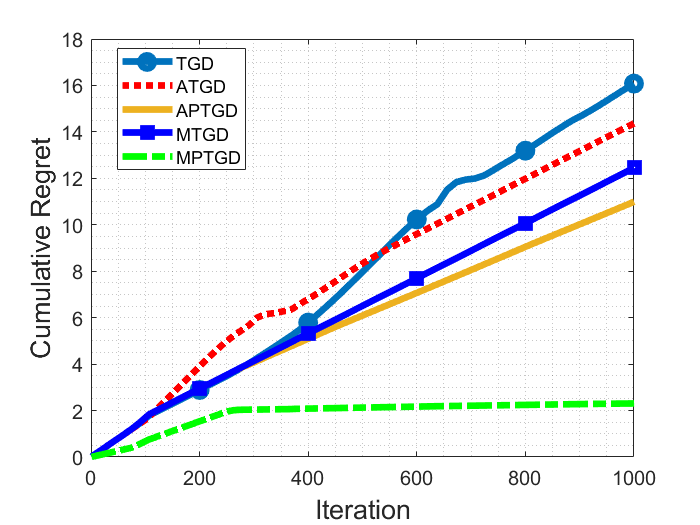
(b)

Figure 3: (a) Local regrets and (b) Cumulative regrets

The next experiment is conducted to show the faster convergence of the proposed algorithms compared to TGD. In each iteration $n$, all of these algorithms require iteratively updating the $x_{m}^{n}$ until the norm of gradient $\|\nabla_{\mathcal{F},\eta}F^{n}_{m,\,w}(x^{n+1}_{m})\|_{2}$ (where $\eta$ is the updated step size at iteration $n$ and varies from different algorithms) is bounded by a certain threshold (for instance, the “while” loop in ATGD describes this process, and the threshold is $\delta$). Alternatively, this experiment implements the algorithms in a reverse setting. It compares the local regrets of all algorithms at the final iteration $N=1000$, given that in each iteration, the number of gradient evaluations is fixed. For MTGD and MPTGD, the number of gradient evaluations for each start $i\in[I]$ equals those of TGD, ATGD, and APTGD. Figure 4 validates that our proposed algorithms have a better local regret than TGD, given the same fixed number of gradient evaluations. For those algorithms to reach a similar local regret, TGD apparently needs more gradient evaluations. As gradient evaluation is normally the most time-consuming step in gradient-based algorithms, our proposed algorithms thus have better computational efficiency. It can also be observed that the perturbed algoritm (MPTGD and APTGD) have a higher local regret than their unperturbed versions (MTGD and ATGD). The possible reason is that the perturbed algorithms are escaping from saddle points when the gradient evaluations stops, so the norm of gradient is relatively high at that moment.

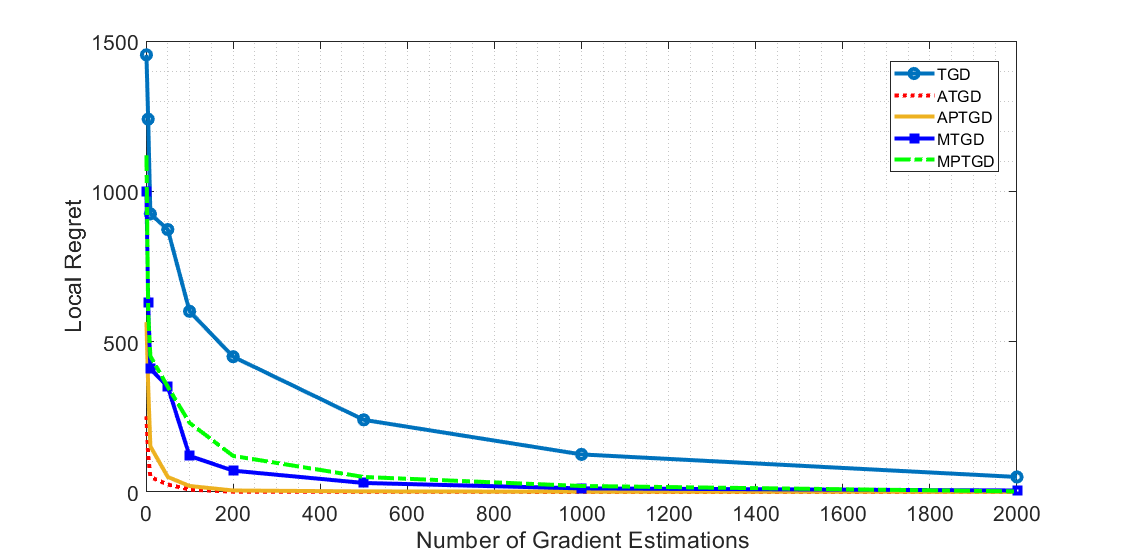
Figure 4: Local regret comparison with fixed gradient estimation

5.2 Sequential Sensor Installation Analysis

In this section, the statistical analysis from Section 3.2 is implemented for the ATGD algorithm. Here, the true pollution source information is $(s,\,l,\,t)=[1300,-22106,-215]$, and the 1000 pairs of artificially generated data are used from sensors in 50 locations. Each round of Algorithm 4 contains 10 iterations, so there will be a total of 100 rounds. Assume that the measurement errors for concentration ($s$), location ($l$), and time ($t$) follow Normal distributions $\mathcal{N}(0,\,50)$, $\mathcal{N}(0,\,500)$ and $\mathcal{N}(0,\,5)$, respectively. The distribution is unknown to the decision maker when implementing Algorithm 4 and ATGD. To compare the performance of Algorithm 4, the “true” required number of sensors is computed by the identification results at the final iteration from $50$ sensors. Here the random measurement errors can be simulated from their given distributions. In the experiments, set $d^{s}=d^{t}=200$ and $d^{l}=500$. Figure 5 shows the minimal number of sensors required in each round and how the number is affected by the initial installation $A$. When $A=3$, the required number already becomes 20 in all later rounds. When $A>=19$, the required number will just be $A$ in later rounds. The optimal policy is to chose a moderate start number (e.g., $A=7,11,13$), and the required number of sensors will finally become $19$. In this experiment, the “true” required number of sensors can be computed and equals 13. So the number of sensors determined by Algorithm 4 is less than two times the “true” number. In addition, the result is insensitive to $A$. By choosing a small number of sensors initially (e.g., $A=3,7$), the required number of sensors determined by Algorithm 4 will already be close to the optimum.

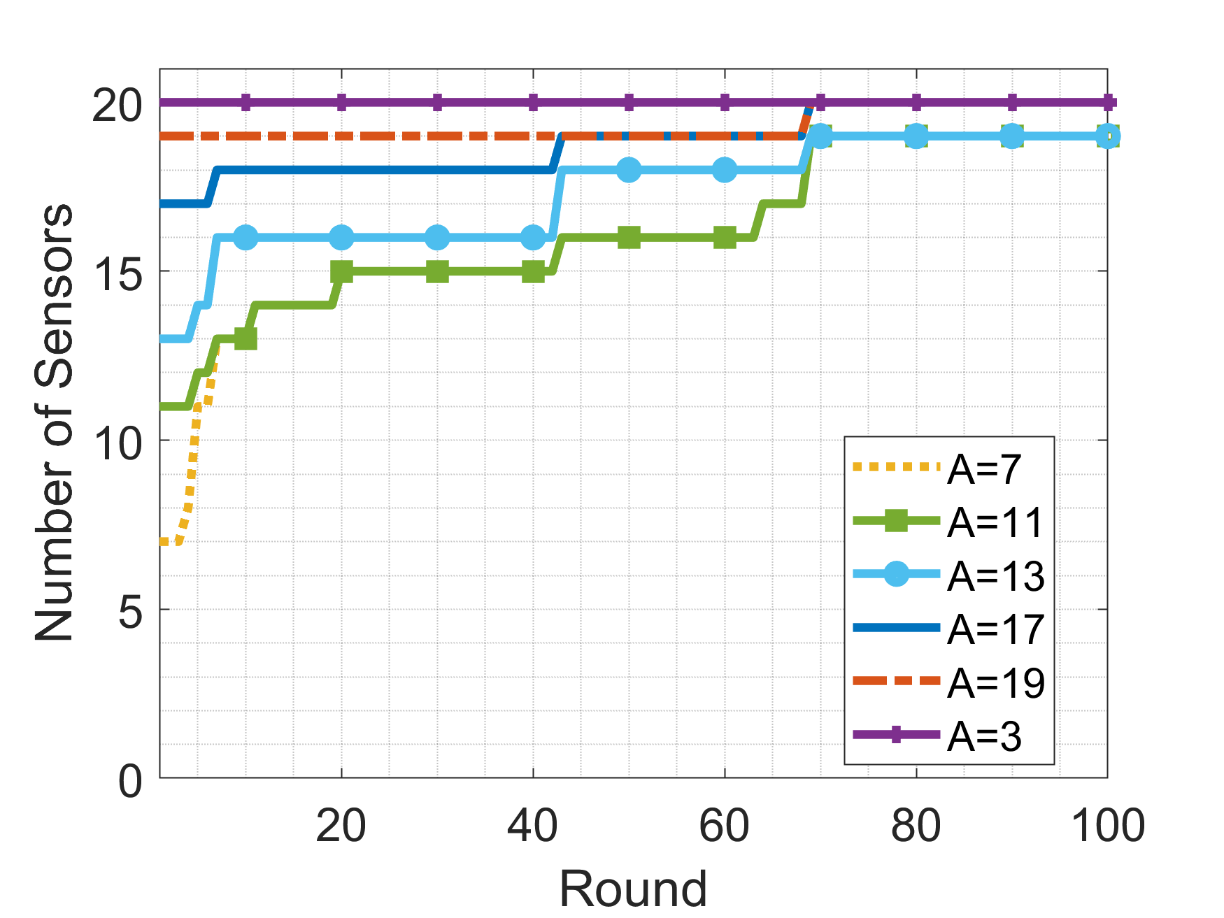
Figure 5: Sequential Sensor installation

5.3 Identification Accuracy and Efficiency

In this section, the computational results and the settings for various online algorithms on the real data are recorded (Table 1). The contents recorded include the estimation result for the pollution source, the estimation error to the true source information, and the average computation time. The initial step size and the parameters in the Backtracking line search are recorded in Table 1. The number of multi-start paths is set to 30. The result shows that the relative error of estimation on each dimension of ATGD and MTGD is (3.46%, 2.79%, and 11.63%). Compared with the estimation result of TGD (3.69%, 4.63%, and 14.42%), ATGD and MTGD improve the estimation results on every dimension. By incorporating the “escaping from saddle points” module, the error is reduced significantly on the released mass estimation, from 3.46% to 1.31%, and the error on the released time estimation is slightly reduced. However, the compensation is that the estimation error on the location estimation is increased to 11.35%. The common shortcoming of TGD, ATGD, APTGD, and MTGD is the high estimation error on the released time estimation. In contrast, MPTGD overcomes this shortcoming by reducing the error significantly, to 1.40%. MPTGD also has the longest computation time, as both the “escaping from saddle points” and multi-start modules are incorporated. Here ATGD, APTGD, MTGD, and MPTGD are all conducted under the initial step sizes $\eta=[110000,11000000,75000]$, which are computed based on the method introduced in Section 3. In terms of computational time, ATGD is more than 10 times faster than TGD, and APTGD is $37\%$ faster than TGD.

Although from Table 1, it seems that there does not exist an algorithm in ATGD, APTGD, MTGD, and MPTGD that “dominates” all others in terms of estimation accuracy in each dimension, the decision-maker can choose to use each algorithm based on their own targets. However, for a real-life problem, the decision maker is recommended to use ATGD and MTGD if the decision maker has a high estimation accuracy requirement on the location estimation, APTGD if the decision maker has a high estimation accuracy requirement on the released mass estimation, and MPTGD if the decision maker has a high estimation accuracy requirement on the released time estimation. Thus, options and guidelines for the decision maker to choose the proper variant of algorithms are provided when they have emphasis on identification accuracy in different dimensions.

Table 1: Computational results and settings

	$(s,l,t)$	Relative Error	Parameter Setting	Time (Second)
TGD	(1348, -23130, -184)	(3.69%, 4.63%, 14.42%)	$\beta=8\times 10^{-6}$	1.1872
ATGD	(1345, -22722, -190)	(3.46%, 2.79%, 11.63%)	$\beta=8\times 10^{-6}$	0.1023
APTGD	(1317, -19597, -191)	(1.31%, 11.35%, 11.16%)	$\beta=2\times 10^{-6}$	0.7471
MTGD	(1345, -22722, -190)	(3.46%, 2.79%, 11.63%)	$\beta=8\times 10^{-6}$, $I=30$	6.0764
MPTGD	(1392, -20994, -212)	(7.00%, 4.78%, 1.40%)	$\beta=2\times 10^{-6}$, $I=30$	21.1709

In addition, the empirical analysis for the number of multi-starts is conducted. Table 2 shows that the relative error on the estimation of the released location ($l$) will decrease significantly as $I$ increases, and the computation time increases linearly as $I$ increases. Table 3 shows that the relative error on the estimation of the released mass ($s$) and location ($l$) decreases as $I$ increases, and the computation time also increases linearly as $I$ increases.

Table 2: Multi-start for MTGD

	$(s,l,t)$	Relative Error	Time (Second)
$I=5$	(2105, -29761, -166)	(61.92%, 34.63%, 22.79%)	2.46
$I=10$	(1315, -29493, -364)	(1.15%, 33.41%, 69.30%)	3.31
$I=15$	(1000, -29463, -166)	(23.08%, 33.28%, 22.79%)	4.17
$I=20$	(1221, -28061, -146)	(6.08%, 26.94%, 32.09%)	5.36
$I=25$	(1234, -17366, -171)	(5.08%, 21.44%, 20.47%)	6.05
$I=30$	(1200, -19686, -200)	(7.69%, 10.95%, 6.98%)	7.09

Table 3: Multi-start for MPTGD

	$(s,l,t)$	Relative Error	Time (Second)
$I=5$	(1394, -20913, -214)	(7.23%, 5.40%, 0.47%)	5.19
$I=10$	(1394, -20916, -214)	(7.23%, 5.38%, 0.47%)	8.79
$I=15$	(1394, -20925, -214)	(7.23%, 5.34%, 0.47%)	12.11
$I=20$	(1394, -20927, -213)	(7.23%, 5.33%, 0.93%)	16.66
$I=25$	(1393, -20930, -213)	(7.15%, 5.32%, 0.93%)	19.49
$I=30$	(1392, -21026, -212)	(7.08%, 4.87%, 1.40%)	22.35

Figure 6 shows that the cumulative regrets of MTGD and MPTGD decrease as the number of multi-starts $I$ increases. For MPTGD, when $I=5,10,15,20,25$, there is a noticeable increase in the cumulative regret, which shows that it is necessary to choose a large $I$ to ensure that there is a high probability of convergence to the global optimum.

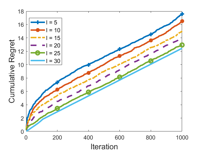
(a)

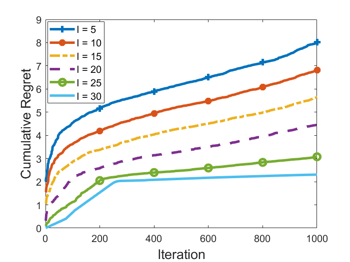
(b)

Figure 6: Empirical analysis of the cumulative regret for multi-start algorithms: (a) MTGD and (b) MPTGD

6 Conclusion

In this paper, novel online non-convex learning algorithms for real-time river pollution source identification problem were developed and analyzed. The identification problem studied in this paper had an instantaneously released pollution source with an initial value on source information identification. Our basic algorithm has vectorized and adaptive step sizes such that it ensured high estimation accuracy in dimensions with different magnitudes (released mass, location and time). In addition, the “escaping from saddle points” module was implemented to form the perturbed algorithm to further improve the estimation accuracy. Our basic algorithm has the local regret $O(N)$, and the perturbed algorithm has the local regret $O(N)$ with a high probability. The high probability cumulative regret bound $O(N)$ under particular condition on loss functions is also shown.

The experiments with artificially generated data validated all our theoretical regret bounds and showed that our algorithms were superior to existing online algorithms in all dimensions (e.g., released mass ($s$), location ($l$), and time ($t$)). Our algorithms were also implemented in Rhodamine WT dye concentration data from a travel time study on the Truckee River between Glenshire Drive near Truckee, California and Mogul, Nevada Crompton (2008). We showed that the multi-start module and “escaping from saddle point” module could achieve a significantly low estimation error in certain dimensions (from 3.69% to 1.21% and from 14.42% to 1.40%). Thus, variants of online algorithms were provided for the decision maker to choose and implement, based on their own estimation accuracy requirement.

For future research, observing that estimating the gradients and project gradients would be computationally demanding especially if the ADE functions are complicated. One possible solution is to develop a “bandit” algorithm. Instead of observing the full information of losses and computing their gradients on the entire domain, only the function value queried by the decision made would be observed, and the limited information would be used to construct an effective estimation of the gradient.

Acknowledgement.

This research was supported by the National Research Foundation (NRF), Prime Minister”s Office, Singapore, under its Campus for Research Excellence and Technological Enterprise (CREATE) program. Wenjie Huang’s research was also supported by the National Natural Science Foundation of China (Grants 72150002), and “HKU-100 Scholars” Research Start-up Funds. The authors are grateful to Professor William B. Haskell and Professor Yao Chen for their valuable comments and suggestions during the preparation of this paper.

Appendix

The supplements of the paper are provided in this section.

Appendix A Multi-start Algorithms

In this section, the multi-start version algorithms (Algorithm 7 and Algorithm 8) are developed based on Algorithm 1 and 5, respectively.

Algorithm 7 MTGD

Input: sensor $m\in M$, window size $w\geq 1$, tolerance $\delta>0$, constant $W,\,K>0$, and a convex set $\mathcal{F}$ and group size $I$;

Set $x^{1}_{m},\,x_{m}^{1,(i)}\in\mathcal{F}$ for $i=1,\,...,\,I$ arbitrarily

for $n=1,\,...,\,N$ do

    Observe the cost function $\Psi^{n}_{m}:\,\mathcal{F}\rightarrow\mathbb{R}$.

    Compute the initial step size: $\eta^{0}=\mathfrak{S}(F^{n}_{m,w},\,K)$.

    for $i=1,\,....,\,I$ do

      Initialize $x_{m}^{n+1,(i)}:=x_{m}^{n,(i)}$.

      Determine $\eta^{n,(i)}$ using Normalized Backtracking-Armijo line search (Algorithm 2) for $x^{n+1,(i)}_{m}$.

         while $\|\nabla_{\mathcal{F},\eta^{n,(i)}}F^{n}_{m,\,w}(x_{m}^{n+1,(i)})\|>\delta$ do

            Update $x_{m}^{n+1,(i)}=x_{m}^{n+1,(i)}-\eta^{n,(i)}\otimes\nabla_{\mathcal{F},\eta^{n,(i)}}F^{n}_{m,\,w}(x_{m}^{n+1,(i)})$.

         end while

   Return $x^{n+1}_{m}\in\arg\min_{x\in\left\{x_{m}^{n+1,(i)}\right\}{}_{i=1,...,I}}\left[\frac{1}{|N_{m}|}\sum_{n\in N_{m}}(C(x|l_{m},\,t_{m}^{n})-c_{m}^{n})\right]^{2}.$

end for

Algorithm 8 MPTGD

Input: sensor $m\in M$, window size $w\geq 1$, constant $c\leq 1$, constant $W,\,K>0$, and a convex set $\mathcal{F}$ and group size $I$;

Input: $\mathcal{\chi}=3\max\left\{\log\left(\frac{d\kappa\triangle f}{c\delta^{2}\epsilon}\right),\,4\right\}$, $r=\frac{\sqrt{c}}{\chi^{2}}\cdot\frac{\delta}{\kappa}$, $g_{\textrm{thres}}=\frac{\sqrt{c}}{\mathcal{\chi}^{2}}\cdot\delta$, $f_{\textrm{thres}}=\frac{c}{\mathcal{\chi}^{3}}\sqrt{\frac{\delta^{3}}{\iota}}$, $t_{\textrm{thres}}=\lceil\frac{\chi}{c^{2}}\cdot\frac{\kappa}{\sqrt{\iota\,\delta}}\rceil$, $t_{\textrm{noise}}=-t_{\textrm{thres}}-1$

Set $x^{1}_{m},\,x_{m}^{1,(i)}\in\mathcal{F}$ for $i=1,\,...,\,I$ arbitrarily

for $n=1,\,...,\,N$ do

   Observe the cost function $\Psi^{n}_{m}:\,\mathcal{F}\rightarrow\mathbb{R}$.

   Compute the initial step size: $\eta^{0}=\mathfrak{S}(F^{n}_{m,w},\,K)$.

   Initialize $t_{\textrm{noise}}$;

   for $i=1,\,....,\,I$ do

      Initialize $x_{m}^{n+1,(i)}:=x_{m}^{n,(i)}$.

      for $t=0,\,1,\,...$ do

         Determine $\eta^{t}$ using Normalized Backtracking-Armijo line search (Algorithm 2).

         Set $x_{m}^{n+1,(i),\>t}=x_{m}^{n,(i)}$.

         if $\|\nabla_{\mathcal{F},\eta^{t}}F^{n}_{m,\,w}(x_{m}^{n+1,(i),\,t})\|\leq\delta$ and $t-t_{\textrm{noise}}>t_{\textrm{thres}}$ then

            $t_{\textrm{noise}}=t$, $\tilde{x}_{m}^{n+1,(i),\,t}=x_{m}^{n+1,(i),\,t}$, $x_{m}^{n+1,(i),\,t}=\tilde{x}_{m}^{n+1,(i),\,t}+\omega$, where $\omega$ uniformly sampled from $\mathbb{B}_{0}(r)$.

         if $t-t_{\textrm{noise}}=t_{\textrm{thres}}$ and $F^{n}_{m,\,w}(x_{m}^{n+1,(i),\,t})-F^{n}_{m,\,w}(x_{m}^{n+1,(i),\,t_{\textrm{noise}}})>-f_{n}^{\textrm{thres}}$ then

            Return $x_{m}^{n+1,(i)}=x_{m}^{n+1,(i),\,t_{\textrm{noise}}}$

         Update $x_{m}^{n+1,(i),\,t+1}=x_{m}^{n+1,(i),\,t}-\eta_{t}\otimes\nabla_{\mathcal{F},\eta_{t}}F^{n}_{m,\,w}(x_{m}^{n+1,(i),\,t})$.

       end for

   end for

   Return $x^{n+1}_{m}\in\arg\min_{x\in\left\{x_{m}^{n+1,(i)}\right\}{}_{i=1,...,I}}\left[\frac{1}{|N_{m}|}\sum_{n\in N_{m}}(C(x|l_{m},\,t_{m}^{n})-c_{m}^{n})\right]^{2}$

end for

Appendix B Supplements for Section 2

Proof of Proposition 2.5: This proposition is proved by first giving the following proposition.

Proposition B.1.

The first and second derivatives of $\tilde{C}_{n,m}$ on the interior of $\mathcal{F}$ are bounded.

Proof.

First, prove the boundedness of first derivative of $\tilde{C}_{n,m}(s,l,t)$ on $(s,\,l,\,t)$. There exist

$$\frac{\partial\tilde{C}_{n,m}(s,l,t)}{\partial s}=\frac{1}{A\sqrt{4\pi D\left(t_{m}^{n}-t\right)}}\exp\left[-\frac{\left(l_{m}-l-v\left(t_{m}^{n}-t\right)\right)^{2}}{4D\left(t_{m}^{n}-t\right)}-k\left(t_{m}^{n}-t\right)\right],$$

$$\frac{\partial\tilde{C}_{n,m}(s,l,t)}{\partial l}=\frac{s}{A\sqrt{4\pi D\left(t_{m}^{n}-t\right)}}\cdot\frac{2\left(l_{m}-l-v\left(t_{m}^{n}-t\right)\right)}{4D\left(t_{m}^{n}-t\right)}\exp\left[-\frac{\left(l_{m}-l-v\left(t_{m}^{n}-t\right)\right)^{2}}{4D\left(t_{m}^{n}-t\right)}-k\left(t_{m}^{n}-t\right)\right],$$

$$\frac{\partial\tilde{C}_{n,m}(s,l,t)}{\partial t}=\frac{4\pi Ds}{2A[4\pi D\left(t_{m}^{n}-t\right)]^{3/2}}\exp\left[-\frac{\left(l_{m}-l-v\left(t_{m}^{n}-t\right)\right)^{2}}{4D\left(t_{m}^{n}-t\right)}-k\left(t_{m}^{n}-t\right)\right]$$

$$\quad+\frac{s}{A\sqrt{4\pi D\left(t_{m}^{n}-t\right)}}\cdot\left[-\frac{(l_{m}-l)^{2}}{4D(t_{m}^{n}-t)^{2}}+\frac{v^{2}}{4D}+k\right]\exp\left[-\frac{\left(l_{m}-l-v\left(t_{m}^{n}-t\right)\right)^{2}}{4D\left(t_{m}^{n}-t\right)}-k\left(t_{m}^{n}-t\right)\right].$$

Based on Assumption 2.3 (ii), for any $t\in\mathcal{T},$ set $t_{m}^{n}-t\neq 0$. It is then clear that the first derivative of $\tilde{C}_{n,m}(s,l,t)$ is continuous. Recall that the feasible set $\mathcal{F}$ is a convex and compact set. By the boundedness of compact sets in a metric space, it can be concluded that the first derivative of $\tilde{C}_{n,m}(s,l,t)$ on $(s,\,l,\,t)$ is bounded. Following the same idea, the boundedness of the second derivatives of $\tilde{C}_{n,m}$ on the interior of $\mathcal{F}$ can be proved. ∎

To prove Proposition 2.5 (i), it is known from Proposition B.1, that the first derivative of $\tilde{C}_{n,m}(x)$ on $\mathcal{F}$ is bounded. From Sohrab (2014), it can be shown that $\tilde{C}_{n,m}(x)$ is Lipschitz continuous on $\mathcal{F}$ with a certain modulus. As $\tilde{C}_{n,m}(x)$ is twice differentiable on $\mathcal{F}$, then the boundedness of the second derivatives from Proposition B.1 leads to the Lipschitz continuity of $\nabla_{x}\tilde{C}_{n,m}$ on $\mathcal{F}$.

Proof of Proposition 2.6: Recall that $\tilde{C}_{n,m}(s,l,t)$ is Lipschitz continuous on the set $\mathcal{F}$ based on Proposition 2.5. Thus, given any $x,\,x^{\prime}\in\mathcal{F}$, it can be shown that $\left\|\tilde{C}_{n,m}(x)-\tilde{C}_{n,m}(x^{\prime})\right\|\leq\sigma\|x-x^{\prime}\|$. As the square function on $\mathcal{F}$ is also Lipschitz continuous, it can be concluded that there exists

$$\left\|(\tilde{C}_{n,m}(x))^{2}-(\tilde{C}_{n,m}(x^{\prime}))^{2}\right\|\leq\kappa_{m}\|\tilde{C}_{n,m}(x)-\tilde{C}_{n,m}(x^{\prime})\|,\forall m\in M.$$

Then, based on the triangle inequality, it can be shown that

$$\left\|\Psi_{m}^{n}(x)-\Psi_{m}^{n}(x^{\prime})\right\| =\left\|(\tilde{C}_{n,m}(x))^{2}-(\tilde{C}_{n,m}(x^{\prime}))^{2}\right\|$$

$$\leq\kappa_{m}\|\tilde{C}_{n,m}(x)-\tilde{C}_{n,m}(x^{\prime})\|$$

$$\leq\kappa_{m}\,\sigma\|x-x^{\prime}\|.$$

Thus, there exists $\kappa=\kappa_{m}\,\sigma,\,\forall m\in M$ such that $\left\|\Psi_{n}(x)-\Psi_{n}(x^{\prime})\right\|\leq\kappa\|x-x^{\prime}\|.$ For (ii) Recall that $\nabla_{x}f$ with $f(x)=x^{2}$ is Lipschitz continuous. For any $x,\,x^{\prime}\in\mathcal{F}$,

$$\|\nabla_{x}(\tilde{C}_{n,m}(x))^{2}-\nabla_{x}(\tilde{C}_{n,m}(x^{\prime}))^{2}\|\leq\tau_{m}\|x-x^{\prime}\|.$$

Based on the triangle inequality,

$$\|\nabla_{x}(\tilde{C}_{n,m}(x))^{2}\|\leq\|\nabla_{x}(\tilde{C}_{n,m}(x^{\prime}))^{2}\|+\tau_{m}\|x-x^{\prime}\|.$$

Fix the value $x^{\prime}\in\mathcal{F}$. As the feasible set of $\mathcal{F}$ is a convex and compact set, $\|\nabla_{x}(\tilde{C}_{n,m}(x))\|$ is bounded; that is, there exists $K_{1m}>0$ such that $\|\nabla_{x}(\tilde{C}_{n,m}(x))\|\leq K_{1m}$. Besides, based on Proposition 2.5, it can be shown that there exists $K_{2m}>0$ such that $\|\nabla_{x}\tilde{C}_{n,m}(x^{\prime})\|\leq K_{2m}$, $\left\|\nabla_{x}\tilde{C}_{n,m}(x)-\nabla_{x}\tilde{C}_{n,m}(x^{\prime})\right\|\leq\gamma\|x-x^{\prime}\|$ and

$$\left\|\nabla_{x}\Psi_{m}^{n}(x)-\nabla_{x}\Psi_{m}^{n}(x^{\prime})\right\|$$

$$= \left\|\nabla_{x}(\tilde{C}_{n,m}(x))^{2}-\nabla_{x}(\tilde{C}_{n,m}(x^{\prime}))^{2}\right\|$$

$$= \left\|\nabla_{x}(\tilde{C}_{n,m}(x))^{2}\nabla_{x}\tilde{C}_{n,m}(x)-\nabla_{x}(\tilde{C}_{n,m}(x^{\prime}))^{2}\nabla_{x}\tilde{C}_{n,m}(x^{\prime})\right\|$$

$$\leq \left\|\nabla_{x}f(\tilde{C}_{n,m}(x))\nabla_{x}\tilde{C}_{n,m}(x)-\nabla_{x}f(\tilde{C}_{n,m}(x^{\prime}))\nabla_{x}\tilde{C}_{n,m}(x^{\prime})\right\|$$

$$= \|\nabla_{x}(\tilde{C}_{n,m}(x))^{2}\nabla_{x}\tilde{C}_{n,m}(x)-\nabla_{x}(\tilde{C}_{n,m}(x))^{2}\nabla_{x}\tilde{C}_{n,m}(x^{\prime})$$

$$+\nabla_{x}(\tilde{C}_{n,m}(x))^{2}\nabla_{x}\tilde{C}_{n,m}(x^{\prime})-\nabla_{x}(\tilde{C}_{n,m}(x^{\prime}))^{2}\nabla_{x}\tilde{C}_{n,m}(x^{\prime})\|$$

$$\leq \left\|\nabla_{x}(\tilde{C}_{n,m}(x))^{2}\right\|\left\|\nabla_{x}\tilde{C}_{n,m}(x)-\nabla_{x}\tilde{C}_{n,m}(x^{\prime})\right\|$$

$$+\left\|\nabla_{x}\tilde{C}_{n,m}(x^{\prime})\right\|\left\|\nabla_{x}(\tilde{C}_{n,m}(x))^{2}-\nabla_{x}(\tilde{C}_{n,m}(x^{\prime}))^{2}\right\|$$

$$\leq (K_{1m}\,\gamma+K_{2m}\tau_{m})\|x-x^{\prime}\|.$$

Let $\beta=\sum_{m\in M}(K_{1m}\,\gamma+K_{2m}\tau_{m})$. Thus, it can be concluded that there exists $\beta$ such that

$$\left\|\nabla_{x}\Psi_{m}^{n}(x)-\nabla_{x}\Psi_{m}^{n}(x^{\prime})\right\|\leq\beta\left\|x-x^{\prime}\right\|.$$

For (iii), given the results in (ii) and implementing the same arguments in (ii), the desired results are derived.

Proof of Proposition 2.8: The proof follows from the proof of (Hazan et al., 2017, Proposition 2.3 ). As $\nabla_{x}\Psi_{m}^{n}(x)$ is a continuous function on $\mathcal{F}$, then the composition function $g(x):=x-\eta\otimes\nabla_{\mathcal{F},\eta}\Psi_{m}^{n}(x)=\Pi_{\mathcal{F}}\left[x-\eta\otimes\nabla_{x}\Psi_{m}^{n}(x)\right]$ is therefore continuous. Thus, $g$ satisfies the conditions for Brouwer’s fixed-point theorem (see Brattka et al. (2016)), implying that there exists some $x^{\ast}\in\mathcal{F}$ for which $g(x^{\ast})=x^{\ast}$. At this point, the projected gradient vanishes.

Proof of Proposition 2.9: See (Hazan et al., 2017, Proposition 2.4). Let $u:=x+\eta\otimes\nabla\Psi(x)$, and $v:=u+\eta\otimes\nabla\Phi(x)$. Define their respective projection $u^{\prime}=\Pi_{\mathcal{F}}[u]$, and $v^{\prime}=\Pi_{\mathcal{F}}[v]$ so that $u^{\prime}=x-\eta\otimes\nabla_{\mathcal{F},\eta}\Psi(x)$, and $v^{\prime}=x-\eta\otimes\nabla_{\mathcal{F},\,\eta}[\Psi+\Phi](x)$. It can be first shown that $\|u^{\prime}-v^{\prime}\|\leq\|u-v\|$.

By the generalized Pythagorean theorem for convex sets, both $\left\langle(u^{\prime}-v^{\prime})\oslash\eta,\,(v-v^{\prime})\oslash\eta\right\rangle\leq 0$ and $\left\langle(v^{\prime}-u^{\prime})\oslash\eta,\,(u-u^{\prime})\oslash\eta\right\rangle\leq 0$ are derived. Combining these, it can be shown that

$$\left\langle(u^{\prime}-v^{\prime})\oslash\eta,\,[u^{\prime}-v^{\prime}-(u-v)]\oslash\eta\right\rangle\leq 0$$

$$\Longrightarrow \|(u^{\prime}-v^{\prime})\oslash\eta\|^{2}\leq\left\langle(u^{\prime}-v^{\prime})\oslash\eta,\,(u-v)\oslash\eta\right\rangle$$

$$\leq\|(u^{\prime}-v^{\prime})\oslash\eta\|\cdot\|(u-v)\oslash\eta\|,$$

as claimed. Finally, by the triangle inequality,

$$\left\|\nabla_{\mathcal{F},\,\eta}[\Psi+\Phi](x)\right\|-\left\|\nabla_{\mathcal{F},\,\eta}\Psi(x)\right\|$$

$$\leq \left\|\nabla_{\mathcal{F},\,\eta}[\Psi+\Phi](x)-\nabla_{\mathcal{F},\,\eta}\Psi(x)\right\|$$

$$= \|(u^{\prime}-v^{\prime})\oslash\eta\|$$

$$\leq \|(u-v)\oslash\eta\|$$

$$= \left\|\nabla\Phi(x)\right\|,$$

as required.

Appendix C Supplements for Section 3

Proof of Theorem 3.1: The theorem holds that the stopping criterion of Algorithm 2 is relaxed from the standard Backtracking-Armijo line search. Explicitly, the termination can also be proved by the limit of the Taylor series. Given the Taylor expansions with respect to the step size $\eta^{(l)}$ for the two terms,

$$F^{n}_{m,\,w}(x^{n+1}_{m}-\eta^{(l)}\otimes\nabla_{\mathcal{F},\eta^{(l)}}F^{n}_{m,\,w}(x^{n+1}_{m})/\|\nabla_{\mathcal{F},\eta^{(l)}}F^{n}_{m,\,w}(x^{n+1}_{m})\|_{2})$$

$$\leq F^{n}_{m,\,w}(x^{n+1}_{m})-\|\eta^{(l)}\|_{\min}\|\nabla_{\mathcal{F},\eta^{(l)}}F^{n}_{m,\,w}(x^{n+1}_{m})\|_{2}+O(\|\eta^{(l)}\|^{2}_{\infty}),$$

and

$$F^{n}_{m,\,w}(x^{n+1}_{m})+\beta\|\eta^{(l)}\otimes\nabla_{\mathcal{F},\eta^{(l)}}F^{n}_{m,\,w}(x^{n+1}_{m})\|_{2}\geq F^{n}_{m,\,w}(x^{n+1}_{m})+\beta\leavevmode\nobreak\ \|\eta^{(l)}\|_{\min}\|\nabla_{\mathcal{F},\eta^{(l)}}F^{n}_{m,\,w}(x^{n+1}_{m})\|_{2}.$$

Obviously, by examining the limit of the two terms when each element of $\eta^{(l)}$ is approaching zero, the condition in Algorithm 2 for entering the “while” loop will be violated, and thus the algorithm will terminate.

Proof of Theorem 3.2: Prove Theorem 3.2 (i) by the following statement. Given that $\eta^{n}$ is computed from Algorithm 2, it can be verified that for all $x\in\mathcal{F}$, and $n\geq 2$, so

$$\|\nabla_{\mathcal{F},\eta^{0}}F_{n-1,\,w}(x)\|_{2}^{2}\leq\|\nabla_{\mathcal{F},\eta^{n}}F_{n-1,\,w}(x)\|_{2}^{2}.$$ (11)

The above equality holds based on the definition of the projected gradient as well as the fact that $\eta^{n}\leq\eta^{0}$. Note that Algorithm 1 only implements an iteration $x^{n}_{m}$ if $\|\nabla_{\mathcal{F},\eta^{n}}F^{n-1}_{m,\,w}(x^{n}_{m})\|_{2}^{2}\leq\delta$. (Note that if $n=1$, $F^{n-1}_{m,\,w}$ is zero.) Let $h^{n}_{m}(x)=\frac{1}{w}\left[\Psi_{m}^{n}(x)-\Psi^{n-w}_{m}(x)\right]$, which is $\frac{2\kappa}{w}$-Lipschitz. Then, for each $1\leq n\leq N$,

$$\|\nabla_{\mathcal{F},\eta^{0}}F^{n}_{m,\,w}(x^{n}_{m})\|_{2}^{2}= \|\nabla_{\mathcal{F},\eta^{0}}\left[F^{n-1}_{m,\,w}+h_{m}^{n}\right](x^{n}_{m})\|_{2}^{2}$$

$$\leq \|\nabla_{\mathcal{F},\eta^{0}}F^{n-1}_{m,\,w}(x^{n}_{m})\|_{2}^{2}+\|\nabla h^{n}_{m}(x^{n}_{m})\|_{2}^{2}$$

$$\leq \|\nabla_{\mathcal{F},\eta^{n}}F^{n-1}_{m,\,w}(x^{n}_{m})\|_{2}^{2}+\|\nabla h^{n}_{m}(x^{n}_{m})\|_{2}^{2}$$

$$\leq (\delta+\frac{2\kappa}{w})^{2}.$$

for any $x\in\mathcal{F}$. The last equality holds based on equality (11), Proposition 2.9, and the stopping criterion of ATGD (Algorithm 1).

To prove Theorem 3.2 (ii), the following lemmas are introduced.

Lemma C.1.

Let $\mathcal{F}$ be a closed convex set, and let $\eta\in\mathbb{R}_{+}^{d}$. Suppose $\Psi:\,\mathcal{F}\rightarrow\mathbb{R}$ is differentiable. Then, for any $x\in\mathbb{R},$

$$\left\langle\nabla\Psi(x),\,\eta^{2}\otimes\nabla_{\mathcal{F},\eta}\Psi(x)\right\rangle\geq\left\|\eta\otimes\nabla_{\mathcal{F},\eta}\Psi(x)\right\|_{2}^{2}.$$

Proof.

Let $u=x-\eta\otimes\nabla\Psi(x)$, and $u^{\prime}=\Pi_{\mathcal{F}}\left[u\right]$. Then

$$\left\langle-\eta\otimes\nabla\Psi(x),\,-\eta\otimes\nabla_{\mathcal{F},\eta}\Psi(x)\right\rangle-\left\|\eta\otimes\nabla_{\mathcal{F},\eta}\Psi(x)\right\|_{2}^{2}$$

$$= \left\langle u-x,\,u^{\prime}-x\right\rangle-\left\langle u^{\prime}-x,\,u^{\prime}-x\right\rangle$$

$$= \left\langle u-u^{\prime},\,u^{\prime}-x\right\rangle\geq 0,$$

where the last inequality follows the generalized Pythagorean theorem. ∎

For $2\leq n\leq N$, let $\tau^{n}$ be the number of gradient steps taken in the outer loop at iteration $n-1$, in order to compute the iteration $x^{n}_{m}$. For convenience, define $\tau^{1}=0$. A progress lemma during each gradient descent epoch is established:

Lemma C.2.

For any $2\leq n\leq N$, there exists $\eta^{\prime}\leq\eta^{0}$ such that

$$F^{n-1}_{m,\,w}(x^{n}_{m})-F^{n-1}_{m,\,w}(x^{n-1}_{m})\leq-\tau^{n}\left(\|\eta^{\prime}\|_{\min}-\frac{\beta\,\|\eta^{0}\|_{\infty}^{2}}{2}\right)\text{$\delta^{2}$}.$$

Proof.

Consider a single iteration $z$ of the loop of $n$, and the next iteration $z^{\prime}:=z-\eta^{n}\otimes\nabla_{\mathcal{F},\eta^{n}}F^{n-1}_{m,\,w}(z)$ occurs when the step size is $\eta^{n}$. This can be shown by the $\beta$-smoothness of $F^{n-1}_{m,\,w}$:

$$F^{n-1}_{m,\,w}(z^{\prime})-F^{n-1}_{m,\,w}(z) \leq\left\langle\nabla F^{n-1}_{m,\,w}(z),\,z^{\prime}-z\right\rangle+\frac{\beta}{2}\|z^{\prime}-z\|_{2}^{2}$$

$$=-\left\langle\nabla F^{n-1}_{m,\,w}(z),\,\eta^{n}\otimes\nabla_{\mathcal{F},\eta^{n}}F^{n-1}_{m,\,w}(z)\right\rangle+\frac{\beta}{2}\|\eta^{n}\otimes\nabla_{\mathcal{F},\eta^{n}}F^{n-1}_{m,\,w}(z)\|_{2}^{2}$$

$$\leq-\|\eta^{n}\|_{\min}\left\|\nabla_{\mathcal{F},\eta^{n}}F^{n-1}_{m,\,w}(z)\right\|_{2}^{2}+\frac{\beta}{2}\|\eta^{n}\otimes\nabla_{\mathcal{F},\eta^{n}}F^{n-1}_{m,\,w}(z)\|_{2}^{2}$$

$$\leq-\left(\|\eta^{\prime}\|_{\min}-\frac{\beta\,\|\eta^{0}\|_{\infty}^{2}}{2}\right)\left\|\nabla_{\mathcal{F},\eta^{n}}F^{n-1}_{m,\,w}(z)\right\|_{2}^{2}.$$

The last equality holds when choosing $\eta^{\prime}\leq\eta^{n}$. The algorithm only takes projected gradient steps when $\|\nabla_{\mathcal{F},\eta^{n}}F^{n-1}_{m,\,w}(z)\|\geq\delta$. Then statement of this lemma can be derived given that $F^{n-1}_{m,\,w}(x^{n}_{m})-F^{n-1}_{m,\,w}(x^{n-1}_{m})=\tau^{n}\left(F^{n-1}_{m,\,w}(z^{\prime})-F^{n-1}_{m,\,w}(z)\right).$ ∎

To complete the proof of the theorem, write the telescopic sum:

$$F^{N}_{m,\,w}(x^{N}_{m}) =\sum_{n=1}^{N}\left[F^{N}_{m,\,w}(x^{n}_{m})-F^{N-1}_{m,\,w}(x_{m}^{n-1})\right]$$

$$=\sum_{n=1}^{N}\left[F^{n-1}_{m,\,w}(x^{n}_{m})-F^{n-1}_{m,\,w}(x^{n-1}_{m})+\Psi^{n}_{m,\,w}(x^{n}_{m})-\Psi^{n-w}_{m,\,w}(x^{n}_{m})\right]$$

$$\leq\sum_{n=2}^{N}\left[F^{n-1}_{m,\,w}(x_{m}^{n})-F^{n-1}_{m,\,w}(x_{m}^{n-1})\right]+\frac{2B\,N}{w}.$$

Using Lemma C.2,

$$F^{N}_{n,\,w}(x^{N}_{m})\leq\frac{2B\,N}{w}-\left(\|\eta^{\prime}\|_{\min}-\frac{\beta\,\|\eta^{0}\|_{\infty}^{2}}{2}\right)\delta^{2}\cdot\sum_{n=1}^{N}\tau^{n},$$

hence,

$$\sum_{n=1}^{N}\tau^{n} \leq\frac{1}{\delta^{2}\left(\|\eta^{\prime}\|_{\min}-\frac{\beta\,\|\eta^{0}\|_{\infty}^{2}}{2}\right)}\cdot\left(\frac{2B\,N}{w}-F^{N}_{m,\,w}(x^{N}_{m})\right)$$

$$\leq\frac{2B}{\delta^{2}\left(\|\eta^{\prime}\|_{\min}-\frac{\beta\,\|\eta^{0}\|_{\infty}^{2}}{2}\right)w}N,$$

as claimed.

Appendix D Supplements for Section 4

Proof of Proposition 4.2: The proposition states that the $\mathcal{F}$ space can be divided into three regions: 1) a region where the gradient is large; 2) a region where the Hessian has a significant negative eigenvalue (around saddle point); and 3) a region close to a local minimum. As $\zeta>0$ can be arbitrarily chosen, the condition in Proposition 4.2 (iii) holds for all $x\in\mathcal{F}$.

Proof of Theorem 4.3: Recall that an $\tilde{\epsilon}$-second-order stationary point has a small gradient, where the Hessian does not have a significant negative eigenvalue. Suppose that currently, at an iteration $x^{n,t}_{m}$ that is not an $\tilde{\epsilon}$-second-order stationary point, there are two possibilities:

1. Gradient is large: $\|\nabla_{x}F^{n}_{m,\,w}(x_{m}^{n,t})\|_{2}\geq g_{\textrm{thres}}$, or

2. Around the saddle point: $\|\nabla_{x}F^{n}_{m,\,w}(x_{m}^{n,t})\|_{2}\leq g_{\textrm{thres}}$ and $\lambda_{\min}\left(\nabla_{x}^{2}F^{n}_{m,\,w}(x_{m}^{n,t})\right)\leq\sqrt{\iota\leavevmode\nobreak\ \tilde{\epsilon}}$.

The following two lemmas address the above two possibilities, which guarantee that the perturbed gradient descent will decrease the function value in both scenarios. The next lemma shows that if the current gradient is large, progress is made in the function value in proportion to the square of the norm of the gradient.

Lemma D.1.

Assume that $\Psi^{n}_{m}$ satisfies the condition in Proposition 2.6. Then, for the gradient descent with the step size $\|\eta\|_{\infty}\leq 1/\kappa$, there exists $\eta^{\prime}\leq\eta$,

$$F^{n}_{m,\,w}(x_{m}^{n,t+1})\leq F^{n}_{m,\,w}(x_{m}^{n,t})-\left(\|\eta^{\prime}\|_{\min}-\frac{\|\eta^{0}\|_{\infty}}{2}\right)\|\nabla_{x}F^{n}_{m,\,w}(x_{m}^{n,t})\|_{2}^{2}.$$

Proof.

By the properties in Proposition 2.6,

$$F^{n}_{m,\,w}(x_{m}^{n,t+1})\leq F^{n}_{m,\,w}(x_{m}^{n,t})+\nabla_{x}F^{n}_{m,\,w}(x_{m}^{n,t})^{\top}(x_{m}^{n,t+1}-x_{m}^{n,t})+\frac{\kappa}{2}\|x_{m}^{n,t+1}-x_{m}^{n,t}\|_{2}^{2}$$

$$\leq F^{n}_{m,\,w}(x_{m}^{n,t})-\|\eta^{t}\|_{\min}\|\nabla_{x}F^{n}_{m,\,w}(x_{m}^{n,t})\|_{2}^{2}+\frac{\kappa\,\|\eta^{t}\|_{\infty}^{2}}{2}\|\nabla_{x}F^{n}_{m,\,w}(x_{m}^{n,t})\|_{2}^{2}$$

$$\leq F^{n}_{m,\,w}(x_{m}^{n,t})-\left(\|\eta^{\prime}\|_{\min}-\frac{\|\eta^{0}\|_{\infty}}{2}\right)\|\nabla_{x}F^{n}_{m,\,w}(x_{m}^{n,t})\|_{2}^{2}$$

∎

The next lemma shows that a perturbation followed by a small number of standard gradient descent steps can also make the function value decrease with a high probability.

Lemma D.2.

There exists an absolute constant $c_{\textrm{max}}$, for $\Psi_{m}^{n}$ satisfies properties in Proposition 2.6 and 4.2, and any $c\leq c_{\textrm{max}}$, and $\chi\geq 1$. Let $\eta_{0},\,r,\,g_{\textrm{thres}},\,f_{\textrm{thres}},\,t_{\textrm{thres}}$ be computed as Algorithm 3. Then, if $\tilde{x}_{m}^{n,t}$ satisfies:

$$\|\nabla_{x}F^{n}_{m,\,w}(\tilde{x}_{m}^{n,t})\|_{2}\leq g_{\textrm{thres}},\quad\textrm{and}\quad\lambda_{\min}\left(\nabla_{x}^{2}F^{n}_{m,\,w}(\tilde{x}_{m}^{n,t})\right)\geq-\sqrt{\iota\,\tilde{\epsilon}},$$

let $x_{m}^{n,t}=\tilde{x}_{m}^{n,t}+\omega_{t}$, where $\omega_{t}$ comes from the uniform distribution over $\mathbb{B}_{0}(r)$, and let $x_{m}^{n,t+1}$ be the iterations of the gradient descent from $x_{m}^{n,t}$ with the step size $\eta^{t}$, with at least the probability $1-\frac{d\,\kappa}{\sqrt{\iota\,\epsilon}}\exp(-\chi)$,

$$F^{n}_{m,\,w}(x_{m}^{n,t+t_{\textrm{thres}}})-F^{n}_{m,\,w}(\tilde{x}_{m}^{n,t})\leq-f_{\textrm{thres}}.$$

In (Jin et al., 2017, Section 5.2) and (Jin et al., 2017, Section A.2 ), detailed proofs have been derived for fixed step-size version of Lemma D.2. The main idea is listed as follows. After adding a perturbation, the current point of the algorithm comes from a uniform distribution over a $d$-dimensional ball centered at $\tilde{x}_{m}^{n,t}$. This perturbation ball can be divided into two adjoined regions: (1) an escaping region, which consists of all the points whose function value decrease by a least $f_{\textrm{thres}}$ after $t_{\textrm{thres}}$ steps; (2) a stuck region. The proof is to show that the stuck region only consists of a small proportion of the volume of the perturbation ball, and the current point has a small chance of falling in the stuck region. The proofs of Lemma D.2 will also hold for vectorized and adjusted step sizes $\eta^{t}$, as $\eta^{t}\leq\eta^{0}$ (see (Jin et al., 2017, Lemma 14, 15, 16 and 17)).

To prove Theorem 4.3 following (Jin et al., 2017, Appendix A), suppose in epoch $n$, the point $x^{0}$ will be the starting point that $\|\nabla_{x}F^{n}_{m,\,w}(x^{0})\|_{2}\leq g_{\textrm{thres}}$. Then, Algorithm 5 will add perturbation and check the termination condition. If the condition is not met, it must follow that

$$F^{n}_{m,\,w}(x_{m}^{{n,t_{\textrm{thres}}}})-F^{n}_{m,\,w}(x^{0})\leq-f_{\textrm{thres}}=-\frac{c}{\chi^{3}}\cdot\sqrt{\frac{\delta^{3}}{\iota}}.$$

This means that on average, every step decreases the function value by

$$\frac{F^{n}_{m,\,w}(x_{m}^{n,{t_{\textrm{thres}}}})-F^{n}_{m,\,w}(x^{0})}{t_{\textrm{thres}}}\leq-\frac{c^{3}}{\chi^{4}}\cdot\frac{\delta^{2}}{\iota},$$

which further means that in each epoch $n$, Algorithm 5 will terminate within the following number of iterations:

$$\frac{\Delta f}{\frac{c^{3}}{\chi^{4}}\cdot\frac{\delta^{2}}{\iota}}=\frac{\chi^{4}}{c^{3}}\cdot\frac{\iota\,\Delta f}{\delta^{2}}=O\left(\frac{\iota\,\Delta f}{\delta^{2}}\log^{4}\left(\frac{d\,\iota\,\Delta f}{\delta^{2}\epsilon}\right)\right).$$

It can also be shown that in each epoch, when Algorithm 5 terminates, the point it finds is actually an $\delta$-second-order stationary point of $F^{n}_{m,w}$. However, during the entire run of Algorithm 5 in each epoch, the number of times the perturbations are added is at most

$$\frac{1}{t_{\textrm{thres}}}\cdot\frac{\chi^{4}}{c^{3}}\cdot\frac{\iota\,\Delta f}{\delta^{2}}=\frac{\chi^{3}}{c}\frac{\sqrt{\iota\,\delta}\Delta f}{\delta^{3}}.$$

Finally, the probability that Algorithm 5 terminates and finds a $\delta$-second-order stationary point is at least

$$1-\frac{d\,\kappa}{\sqrt{\iota\,\epsilon}}\exp(-\chi)\frac{\chi^{3}}{c}\frac{\sqrt{\iota\,\delta}\Delta f}{\delta^{3}}\geq 1-\delta,$$

given the formulation of $\chi$.

Proof of Theorem 4.7: With probability $1-\epsilon$, and after

$$O\left(\frac{\kappa\triangle f\,w^{2}}{\delta^{2}}\log^{4}\left(\frac{d\kappa\triangle fw^{2}}{\delta^{2}\epsilon}\right)\,N\right),$$

gradient estimations, the long-run average cumulative regret, denoted by $\mathfrak{R}^{G}_{m}$, is as follows until time $N$ is

$$\frac{\mathfrak{R}^{G}_{m}(N)}{N}= \frac{1}{N}\left[\sum_{n=1}^{N}\Psi_{m}^{n}(x_{m}^{n})-\inf_{x\in\mathcal{F}}\sum_{n=1}^{N}\Psi_{m}^{n}(x)\right]$$

$$\leq \frac{1}{N}\left[\sum_{n=1}^{N}\Psi_{m}^{n}(x_{m}^{n})-\sum_{n=1}^{N}\Psi_{m}^{n}(x_{m}^{n,\ast})\right]$$

$$\leq \frac{\mu}{\kappa}\frac{1}{N}\sum_{n=1}^{N}\|\nabla_{x}\Psi^{n}_{m}(x_{m}^{n})\|$$

$$= \frac{\mu\delta}{\kappa}.$$

Assumption 4.6 can be ensured with a high probability. The probability of attaining the cumulative regret bound is thus no higher than $1-\epsilon$.

References

- Abubakar et al. (2015) Abubakar, I., Khalid, S., Mustafa, M., Shareef, H., and Mustapha, M. (2015). An overview of non-intrusive load monitoring methodologies. In 2015 IEEE Conference on Energy Conversion (CENCON), pages 54–59. IEEE.
- Agarwal and Niyogi (2009) Agarwal, S. and Niyogi, P. (2009). Generalization bounds for ranking algorithms via algorithmic stability. Journal of Machine Learning Research, 10(Feb):441–474.
- Armijo (1966) Armijo, L. (1966). Minimization of functions having Lipschitz continuous first partial derivatives. Pacific Journal of mathematics, 16(1):1–3. Publisher: Mathematical Sciences Publishers.
- Brattka et al. (2016) Brattka, V., Le Roux, S., Miller, J. S., and Pauly, A. (2016). The brouwer fixed point theorem revisited. In Conference on Computability in Europe, pages 58–67. Springer.
- Carlsen et al. (2008) Carlsen, S., Skavhaug, A., Petersen, S., and Doyle, P. (2008). Using wireless sensor networks to enable increased oil recovery. In 2008 IEEE international conference on emerging technologies and factory automation, pages 1039–1048. IEEE.
- Chesher (1991) Chesher, A. (1991). The effect of measurement error. Biometrika, 78(3):451–462.
- Chinrungrueng et al. (2006) Chinrungrueng, J., Sununtachaikul, U., and Triamlumlerd, S. (2006). A vehicular monitoring system with power-efficient wireless sensor networks. In 2006 6th International Conference on ITS Telecommunications, pages 951–954. IEEE.
- Coskun and Oosterhuis (2020) Coskun, A. and Oosterhuis, W. P. (2020). Statistical distributions commonly used in measurement uncertainty in laboratory medicine. Biochemia medica, 30(1):5–17.
- Crompton (2008) Crompton, E. J. (2008). Traveltime for the Truckee River between Tahoe City, California, and Vista, Nevada, 2006 and 2007. USGS Numbered Series 2008-1084, Geological Survey (U.S.).
- De Smedt et al. (2005) De Smedt, F., Brevis, W., and Debels, P. (2005). Analytical Solution for Solute Transport Resulting from Instantaneous Injection in Streams with Transient Storage. Journal of Hydrology, 315(1-4):25–39.
- Dennis Jr and Schnabel (1996) Dennis Jr, J. E. and Schnabel, R. B. (1996). Numerical methods for unconstrained optimization and nonlinear equations, volume 16. Siam.
- Dong et al. (2017) Dong, X., Cheng, L., Zheng, G., and Wang, T. (2017). Deployment cost minimization for composite event detection in large-scale heterogeneous wireless sensor networks. International Journal of Distributed Sensor Networks, 13(6):1550147717714171.
- Drusvyatskiy and Lewis (2018) Drusvyatskiy, D. and Lewis, A. S. (2018). Error Bounds, Quadratic Growth, and Linear Convergence of Proximal Methods. Math. Oper. Res., 43(3):919–948.
- Fuller (1995) Fuller, W. A. (1995). Estimation in the presence of measurement error. International Statistical Review/Revue Internationale de Statistique, pages 121–141.
- Gao et al. (2018) Gao, X., Li, X., and Zhang, S. (2018). Online Learning with Non-Convex Losses and Non-Stationary Regret. In Storkey, A. J. and Peérez-Cruz, F., editors, International Conference on Artificial Intelligence and Statistics, AISTATS 2018, 9-11 April 2018, Playa Blanca, Lanzarote, Canary Islands, Spain, volume 84 of Proceedings of Machine Learning Research, pages 235–243. PMLR.
- Ge et al. (2015) Ge, R., Huang, F., Jin, C., and Yuan, Y. (2015). Escaping From Saddle Points — Online Stochastic Gradient for Tensor Decomposition. arXiv: http://arxiv.org/abs/1503.02101v1.
- Gimbutas and Žilinskas (2016) Gimbutas, A. and Žilinskas, A. (2016). On global optimization using an estimate of Lipschitz constant and simplicial partition. In AIP Conference Proceedings, volume 1776, page 060012. AIP Publishing. Issue: 1.
- Guo and Cheng (2019) Guo, G. and Cheng, G. (2019). Mathematical modelling and application for simulation of water pollution accidents. Process Safety and Environmental Protection, 127:189–196.
- Hazan (2016) Hazan, E. (2016). Introduction to Online Convex Optimization. Foundations and Trends in Optimization, 2(3-4):157–325.
- Hazan et al. (2017) Hazan, E., Singh, K., and Zhang, C. (2017). Efficient Regret Minimization in Non-Convex Games. In Precup, D. and Teh, Y. W., editors, Proceedings of the 34th International Conference on Machine Learning, ICML 2017, Sydney, NSW, Australia, 6-11 August 2017, volume 70 of Proceedings of Machine Learning Research, pages 1433–1441. PMLR.
- Hazart et al. (2014) Hazart, A., Giovannelli, J.-F., Dubost, S., and Chatellier, L. (2014). Inverse Transport Problem of Estimating Point-like Source Using a Bayesian Parametric Method with MCMC. Signal Processing, 96(PB):346–361.
- Jha and Datta (2012) Jha, M. and Datta, B. (2012). Three-dimensional groundwater contamination source identification using adaptive simulated annealing. Journal of Hydrologic Engineering, 18(3):307–317.
- Ji et al. (2017) Ji, L., Liu, J., Li, Z., Pan, B., and Sun, M. (2017). Accidents of Water Pollution in China in 2011-2015 and Their Causes. Journal of Ecology and Rural Environment, 33(9):775–782.
- Jiang et al. (2017) Jiang, J., Dong, F., Liu, R., and Yuan, Y. (2017). Applicability of Bayesian Inference Approach for Pollution Source Identification of River Chemical Spills: A Tracer Experiment Based Analysis of Algorithmic Parameters, Impacts and Comparison with Frequentist Approaches. China Environmental Science, 37(10):3813–3825.
- Jiang et al. (2015) Jiang, M., Huang, W., Huang, Z., and Yen, G. G. (2015). Integration of global and local metrics for domain adaptation learning via dimensionality reduction. IEEE transactions on cybernetics, 47(1):38–51. Publisher: IEEE.
- Jin et al. (2017) Jin, C., Ge, R., Netrapalli, P., Kakade, S. M., and Jordan, M. I. (2017). How to Escape Saddle Points Efficiently. In Precup, D. and Teh, Y. W., editors, Proceedings of the 34th International Conference on Machine Learning, ICML 2017, Sydney, NSW, Australia, 6-11 August 2017, volume 70 of Proceedings of Machine Learning Research, pages 1724–1732. PMLR.
- Kelly (2007) Kelly, B. C. (2007). Some aspects of measurement error in linear regression of astronomical data. The Astrophysical Journal, 665(2):1489.
- Levin (2006) Levin, J. (2006). Choice under uncertainty. Lecture Notes.
- Li and Mao (2011) Li, Z. and Mao, X.-z. (2011). Global multiquadric collocation method for groundwater contaminant source identification. Environmental Modelling, page 11.
- Li et al. (2016) Li, Z., Mao, X.-Z., Li, T. S., and Zhang, S. (2016). Estimation of river pollution source using the space-time radial basis collocation method. Advances in Water Resources, 88:68–79.
- Luo and Tseng (1993) Luo, Z.-Q. and Tseng, P. (1993). Error bounds and convergence analysis of feasible descent methods: a general approach. Annals of Operations Research, 46(1):157–178. ISBN: 1572-9338 Publisher: Springer.
- Maillard and Munos (2010) Maillard, O.-A. and Munos, R. (2010). Online Learning in Adversarial Lipschitz Environments. In Balcázar, J. L., Bonchi, F., Gionis, A., and Sebag, M., editors, Machine Learning and Knowledge Discovery in Databases, European Conference, ECML PKDD 2010, Barcelona, Spain, September 20-24, 2010, Proceedings, Part II, volume 6322 of Lecture Notes in Computer Science, pages 305–320. Springer.
- Milne (2018) Milne, T. (2018). Piecewise strong convexity of neural networks. arXiv preprint arXiv:1810.12805.