Pricing Barrier Options with DeepBSDEs
Abstract
This paper presents a novel and direct approach to price boundary and final-value problems, corresponding to barrier options, using forward deep learning to solve forward-backward stochastic differential equations (FBSDEs). Barrier instruments are instruments that expire or transform into another instrument if a barrier condition is satisfied before maturity; otherwise they perform like the instrument without the barrier condition. In the PDE formulation, this corresponds to adding boundary conditions to the final value problem. The deep BSDE methods developed so far have not addressed barrier/boundary conditions directly. We extend the forward deep BSDE to the barrier condition case by adding nodes to the computational graph to explicitly monitor the barrier conditions for each realization of the dynamics as well as nodes that preserve the time, state variables, and trading strategy value at barrier breach or at maturity otherwise. Given these additional nodes in the computational graph, the forward loss function quantifies the replication of the barrier or final payoff according to a chosen risk measure such as squared sum of differences. The proposed method can handle any barrier condition in the FBSDE set-up and any Dirichlet boundary conditions in the PDE set-up, both in low and high dimensions.
1 Introduction
Deep Learning and Deep Neural Networks have been applied to numerically solve high-dimensional nonlinear PDEs via the use of Forward-Backward Stochastic Differential Equations or FBSDEs (see [HJE18]). In particular, they applied it to a quantitative finance pricing problem to price a combination of two call options under differential rates (dfferent lending and borrowing interest rates), a nonlinear problem that was also studied in [Mer15]. In related work, [CWNMW19] and [Rai18] also showed the applicability of deep learning in solving FBSDEs. The overview paper of Deep BSDE methods [Hie19] introduces how FBSDE and certain deep learning methods can be used to solve quantitative finance problems beyond options pricing to general contingent claims, hedging and initial margin problems.
This paper presents a novel approach to price boundary and final value problems (corresponding to barrier options) with forward deep learning approaches (“forward deep BSDE”). The approach adds nodes to the computational graph of the deep neural network to explicitly monitor the barrier conditions for each realization of the dynamics. In case of barrier breach, the nodes record the time and underlying state variables; otherwise they record the final time and value at maturity which is used to determine the final payoff. The forward loss function then quantifies the replication of the barrier or final payoff according to a chosen risk measure such as squared sum of differences.
The simplest forms of barrier options are single-underlier or basket knock-in or knock-out options in which the barrier condition only involves the current value of the underlier or the basket and compares it to a given barrier level, which is often a given constant. Let be that underlier or the value of the basket. Examples shown in Table 1 include the variants of simple Barrier calls in this setting, for strike price (), time to maturity (), a barrier positions and (possibly time dependent) and the vanilla call price . Put versions of these examples are obtained by replacing calls and call prices by puts and put prices everywhere.
| Name | Barrier Condition | Knocked-in Instrument Rebate | Knocked-In Instrument Value | Final Payoff if not breached |
|---|---|---|---|---|
| Up-and-Out Call | (Upper Barrier Position) | |||
| Down-and-Out Call | (Lower Barrier Position) | |||
| Up-and-In Call | (Upper Barrier Position) | |||
| Down-and-In Call | (Lower Barrier Position) |
The simplest barrier options are those with barrier at some constant level which is active for the entire life of the instrument. Two standard examples: A standard Up-and-Out barrier call option with upper barrier will pay the final call payoff unless the underlier of the option was observed at a level during the life of the option in which case it will pay a rebate . A standard up-and-in barrier call option with upper barrier will pay the final call payoff only if the underlier of the option was observed at a level during the life of the option and otherwise will pay a rebate .
Given a knocked-in instrument, a model, and a valuation approach applied to that model, the knocked-in instrument can be replaced by an immediate payment of the value of the knocked-in instrument according to the model. In this way, one can restrict oneself to the case of knock-out instruments with rebates.
There are many instruments with barrier features in Quantitative Finance. There are also many other applications in natural sciences, engineering, and economics that involve bounded domains and boundaries in stochastic analysis and stochastic processes. Similarly, PDE models in natural sciences and engineering are often posed in bounded domains with boundary conditions imposed at the boundary. The extensions presented in this paper to the forward deep BSDE method allow this new methodology to be applied to all these situations and applications.
The rest of the paper is organized as follows: Section 2 presents a brief overview of Forward-Backward Stochastic Differential Equations as applied to options pricing. Section 3 discusses the technique behind DeepBSDE approach to solving traditional Option pricing problem and a description of the approach to problems with barriers. Section 4 discusses other approaches that are currently used or proposed to pricing Barrier Options and outlines their limitations. Section 5 describes our approach, which employs barrier tracking variables as a part of the DeepBSDE network. Section 6 presents the results of pricing different types of barrier options using this approach and error convergence. The paper concludes with some remarks.
2 Problem Setup and Forward-Backward SDEs
For a general introduction to FBSDE and their relations to nonlinear parabolic PDE and/or quantitative finance, see [EKPQ97] and [Per10]. [HJE18] presented the first application of DeepBSDE method to the pricing of European options under differential rates. [Hie19] provides an overview of the types of problems in quantitative finance that can be solved using deepBSDE and FBSDE. In this paper, we will discuss only specific aspects of PDEs and FBSDEs relevant to our setting.
We will first discuss how a semilinear parabolic PDE can give rise to a FBSDE. A semilinear parabolic PDE is a PDE of the form:
| (1) | |||||
defined on a domain and . In quantitative finance and other applications, these PDE are often posed with terminal conditions, for a given function . However, the case where boundary/barrier conditions
| (2) |
are imposed is also of interest. Final value conditions can be included so that with the previously defined . We assume that this is done.
Consider an Itô process given by:
| (3) |
where and , with uncorrelated and correlations expressed through . For every we will consider a version of that starts (or arrives) at time in and call it . Let be . Then satisfies the Backward Stochastic Differential Equation
| (4) |
along with the equation for , satisfying (3). A terminal condition for the PDE translates into a terminal condition for the BSDE .
With , the BSDE (4) can be written
| (5) |
Equations (3) and (5) together describe the dynamics of solution of PDE (1) within the framework of FBSDE. So, instead of solving a PDE (1) for , we can solve the FBSDE (5) by finding stochastic processes and . Instead of finding a process we can also try to find a function (or different functions for different ) such that , as inspired by the expression for given above.
Notice that the FBSDE as written in (3) and (5) can be more general than the original PDE. For instance, the terminal condition could be a random variable rather than a function, depending on the path of rather than just the final value. Then, solution functions and portfolio functions would also have more general forms and more arguments and might also depend on additional processes that capture the path-dependency of the terminal condition.
The above relation between PDE and FBSDE can be illustrated explicitly, for instance in the case of risk-neutral valuation of simple derivatives which obey the Black-Scholes-Merton equation
| (6) |
with the underlying , driven by the Itô process, in the risk-neutral measure [Shr04], under which follows
| (7) |
where is the risk-free rate and is the volatility of the underlier. Under this setup, for any function , by Itô process rule,
| (8) |
If is to describe the behavior of the value of the derivative , it has to obey equation (6), along with the terminal condition, . Under this assumption (6), the first term on right side in the paranthesis of equation(8) must obey,
| (9) |
substituting for the term above in equation(8), leads to the update equation for :
| (10) |
Now denoting , , , and , this update equation corresponds to (5).
To include the barrier condition in the FBSDE formulation, the process that we are trying to determine will follow the FBSDE (3) and (5) when is outside of while the value of the process is directly given by inside of .111We will not discuss the behavior of or close to the boundary, we will just assume that boundary conditions are consistent and the appropriate conditions are satisfied so that and/or will satisfy those boundary conditions in the appropriate sense.
There are many additional variants, such as multiple barrier conditions, barrier conditions only active at certain discrete times or in certain time intervals, etc. At a more general level, a FBSDE problem with barrier conditions can be stated as follows:
Define the condition (eg: the barrier breach) as a random variable with values and which is measurable (computable) given the information about the dynamics . At the time the condition turns , it is ‘stopped’ and will stay for all subsequent times.
- i.
-
ii.
If is , is equal to or approximates a given final value (in general, a random variable measurable at time ).
-
iii.
If is , is equal to or approximates a given barrier value (in general, a random variable measurable as of time ).
-
iv.
For the up-and-out barrier mentioned above for a single underlier, , the condition is whether is true or false (which gives the barrier region as the domain where and the boundary as ), is zero, and is the standard call payoff.
In the case that the final value is given as function of and barrier conditions and values are given as functions of time and the ‘state variables’ at that time, , this time-continuous FBSDE problem, under appropriate conditions, is equivalent to a PDE boundary/final value problem where the final values are given by that function , the boundary values are given by that function , and the boundary region is defined by the (boundary of the) domain in which is true.
For the up-and-out barrier mentioned previously, these conditions are satisfied and one obtains the same PDE as before, only with a zero boundary condition enforced on . For any general FBSDE problem as in Equations (3) and (5), applying a simple Euler-Maruyama discretization for both and , we obtain
| (11) |
| (12) |
This can be used to time-step both and forward.
3 Solving BSDE with Deep Neural Networks
We will first discuss application to European option pricing (see [HJE18]). The FBSDE is first discretized in time as in (11) and (12). The portfolio process is represented by functions , one for each time , and each function is given as a deep neural network. The initial value of the portfolio at the fixed and the initial portfolio composition are given as constants.
To generate a realization/training sample, one first generates a realization of by (11) and then given the current parameter values for and all the networks, one computes and finally step by step by (12). The norm of the replication error was used as a loss function.
Instead of using a constant , one can start with a randomly generated
. Under those circumstances, one determines the parameters of the network
representing the function rather than a single value (and also
a network and its parameters). We have also implemented that
method. [HJE18] mention the forward approach for random as a
possibility on page 8509 but we are not aware of any implementation of this
method besides our own to the best of our knowledge. One can also use other risk
measures defined from the replication error in the optimization. Finally, the
loss function is optimized with stochastic optimization methods such as
mini-batch stochastic gradient descent combined with Adam optimizers or other
appropriate deep learning methods to determine the parameters of the and
network.
Figure 1 shows the computational graph for the forward
method for European options with random .
As seen earlier, in the time-continuous case, , which in financial terms corresponds to delta-hedging according to some value function . In the case the FBSDE, time-continuous or not, is expressed as minimization, the determined during the optimization does not necessarily have to be equal to although it often approximates it to a certain extent. In the time-discrete case, the analytical solution is no longer guaranteed to minimize the replication error, but reflects a good benchmark and what one would achieve by delta-hedging with that value function. Later, in section 6.1, we will compare the hedging/replication strategy given by the optimized DNN with the one implied by the analytical solution, for the barrier case.
We now present the fundamental idea for the barrier case and will leave the implementation details to a later section. The fundamental idea to extend the forward method to the barrier case is that the barrier breach time and place (together with maturity) takes the place of maturity as the first time and place at which the value of is known and any approximation of should try to approximate that first known value well regardless whether it was specified in the problem as a final value or a barrier condition value.
The first time at which the dynamics enters the barrier domain or satisfies the barrier condition is called barrier touch/breach time. With the version of started in at time , we denote as the first time when the barrier is breached (when is first true). As previously mentioned, we add the set to the barrier domain and set the barrier value function to the final value function at maturity and denote the resulting stopping time as (since both barrier domain and stopping time depend now on T) and also note that is the minimum of and .
Thus, the loss function to be minimized, according to some norm/risk masure (for instance, norm), is
| (13) |
4 Other Approaches to Pricing Barrier Options
We briefly review some of the techniques used in practice to price such barrier options.
PDE Based Approaches: Options pricing via the solution of PDE with finite differences or finite elements or other standard approaches in high dimensions (many underlying assets) poses difficulties due to extreme storage and computational requirements to compute and store the values on a grid that covers the domain. Accuracy and stability requirements often require larger grids than what is achievable with given resources. In traditional PDE schemes, the PDE grid is generated with sufficiently small spacing for finite difference methods in region of interest that includes final time and barrier positions. The finite difference time-stepping proceeds from the final time along the time axis spanning a domain bounded on one or both sides by barriers and/or other appropriate boundary conditions. The time-stepping scheme is then applied to determine the values at grid points going backward in time. PDE techniques are well studied and applied widely, however their applicability is limited and is best suited to pricing derivatives on fewer number of underliers due to issues with storage and computational requirements caused by dimensionality. However, PDE techniques can model at least some nonlinear pricing.
Monte-Carlo Based Approaches: Barrier options in high dimensions are often priced by Monte-Carlo approaches. This includes generating multiple independent sample paths of the underliers in order to compute the realized payoff at maturity or barrier breach along each path and discounting it to the present time and averaging the payoffs to determine the value of the option. While generating sample paths in high dimensions certainly increases in difficulty and resource requirements with the dimension, these requirements do not depend exponentially on the number of dimensions as the grid size in PDE. In the case when there are rare events with high impact on the price (such as a knock-out condition on a short or far out barrier for an otherwise high payoff), simulation-based approaches such as Monte-Carlo need to sample those rare events sufficiently well to approximate the price of the instrument well. One of the main limitations of standard Monte-Carlo based approaches is that they can only take into account risk-neutral discounting or other linear pricing approaches and cannot be used to model nonlinear pricing such as the differential rates, in which borrowing and lending attracts different interest rates [Hie19].
DeepBSDE Based Approaches: DeepBSDE based approaches as originally proposed in [HJE18] alleviate the problem of dimensionality by converting the high-dimensional PDEs into Backward Stochastic Differential Equations. The SDEs are then solved as a stochastic optimal control problem by approximating the co-state and initial value of the control problem using Deep Neural Networks. In the present work we apply this technique to price Barrier options.
Barrier options require the handling of the barrier boundary conditions as they correspond to ‘knock-in’ and ‘knock-out’s at any time before maturity and such problems are not treated in [HJE18].
For risk neutral barrier option pricing, the following expression holds
| (14) |
where the expectation is taken with respect to the risk-neutral measure [Shr04]. Under the risk-neutral measure, the value of at time is equal to expectation of with discounted back to with the risk free interest rate. Under this risk-neutral measure follows (7) with functions as defined in Section 2, denotes the earlier of barrier breach and maturity, and combines both final values and barrier values, as defined in Section 3. For knock-out options with zero rebate, will be zero unless .
Therefore, (14) will in this case simplify to
| (15) | |||||
This corresponds to an instrument with final payoff
| (16) |
which is measurable as of time knowing up to that time . In the case that can be written as a (relatively simple and explicit) function of and , this will give a (different) final value problem for each and . Informally, the final payoff function is adapted via a Brownian bridge based method to include the probability of breaching the barrier before option maturity.
In recent work, [YXS19] have approached the Barrier option pricing as described by the above formula. The computation of probability of breach as a function of , , , and is analytically tractable for constant barriers and simple risk models (constant drift and volatility of the underlying assets), with the help of results from Brownian bridge probabilities. Once and are fixed, these are standard final value problems that can be solved with the deep BSDE methods for European options, as demonstrated in [YXS19].
A slight generalization can be derived along similar lines for the case in which touching the barrier does not lead to an immediate rebate but only to a changed final payoff, which we denote by . Proceeding similarly to above, one obtains an expectation that can be interpreted as an European option on the final payoff
| (17) |
However, in general, time varying barriers and stochastic risk-models
(stochastic interest-rate and volatility of underliers) require Monte-Carlo
based approaches to compute the probability. For instance for a single barrier
with different levels in multiple time-periods, the probability computation can
be extended as follows:
Consider an Up-and-Out barrier option with piecewise constant barriers with
values within , defined by increasing times ,
,…, :
| (18) |
The total probability of no-breach can be computed as product of probabilities of no-breach within each time period, informally written as:
| (19) | |||||
whereeach of the probability values can be computed via Brownian bridge for simple risk-models. However, now one needs to integrate over and/or otherwise sample over the intermediate positions at intermediate times to obtain the barrier probabilities as a function of only initial and final risk factor value. Some other popular varieties of barrier options including multiple barriers (Up and Down Barriers), interacting barriers and barriers specified as a function of asset price (maximum drawdown) require more involved Monte-Carlo approaches to compute the probability. Monte-Carlo approaches in higher dimensions to compute these probability are computationally expensive and incur higher costs than pricing the option in higher dimensions as outlined above (and therefore will not lead to an efficient method to compute barrier option values through final value problems).
In this work, we propose an original approach using DeepBSDEs that explicitly monitors whether the underliers breach the barrier before maturity and record the state of the barrier option at every time step via nodes in the computational graph, which is then used to determine the appropriate payoff conditions. The technique proposed here is applicable to solving general semi-linear parabolic PDEs or FBSDE in any discipline (in addition to quantitative finance) in which boundary conditions are specified. To the best of our knowledge there is no prior work to handle boundary conditions explicitly in the context of DeepBSDEs, which is important in solving a variety of PDEs and FBSDE with standard and non-standard boundary conditions.
5 Deep Neural Network with Barrier Triggers
As mentioned before, we need to keep track of variables that detect whether the barrier was breached (the barrier condition satisfied) and preserve the value of , , and at the time of the first barrier breach. In general, we will call these “conditional” variables, or “conditional” tensors (since variables are represented as and called tensors in TensorFlow).
In the time-continuous setting, we need the values of , , and to compute the loss function (13) or some other risk measure that evaluates how the trading strategy replicates the appropriate payoff. In the time-discrete case, we need to keep track of time-discrete counterparts, which we call ( for payoff), ( for payoff), and ( for payoff). To write updates for these variables, we need that turns from false (0.0) to true (1.0) once the barrier has been breached. For barrier condition functions , this can be defined as
| (20) |
For a problem with a single upper barrier at level active during the entire time to maturity, this would read
| (21) |
would be appropriately initialized depending on whether the barrier condition will be checked at time and could possibly be true there or whether it will only be checked starting at the next time step.
Having defined , we can define , , and as follows:
| (22) | |||||
| (23) | |||||
| (24) |
and initialized with , , and . These update equations keep copying the underlying , , and until the barrier is hit and then stop at the next step, so that the values of the corresponding variables at barrier breach stay in the *FP versions. If the barrier is never breached, the values of , , and at will be in , , and . Thus, , , and are the appropriate time-discrete analogues of , , and , and the loss function for the computational graph implementing this time-discrete approach would be
| (25) |
or any other appropriate risk measure.
Notice also that time-discretization leads to well-known biases in barrier options. If approximation of a certain time-continuous problem with continuously enforced barriers is desired, there are approaches such as barrier level correction (solving the time-discrete problem with appropriately shifted barrier levels) that will minimize such bias and lead to faster convergence to the solution of the time-continuous problem.
Figure 2 shows the computational graph/network for the approach just described. The variables/tensors that have been added or changed for the barrier case are shown as color shaded nodes and the nodes from the original forward deep BSDE network are shown unshaded. As discussed above, these additional tensors are needed to preserve the state at barrier breach or maturity and serve to constrain the appropriately so that it follows the FBSDE if not in the barrier domain but approximates the given barrier domain value once it touches the barrier domain.
The function will encode the specific barrier option treated. For a knock-out barrier call option, the barrier and final payoff is given by
| (26) |
A knock-in barrier call option would be given by
| (27) |
with the vanilla call price (as also used in the introduction section). For both examples, we assume that the barrier is not active at . Note that the given is the same regardless of the level or number of barriers and can be thus used for up-and-out respective up-and-in, down-and-out respective down-and-in, and the double barrier variants of each.
5.1 Behavior of the Conditional Tensors
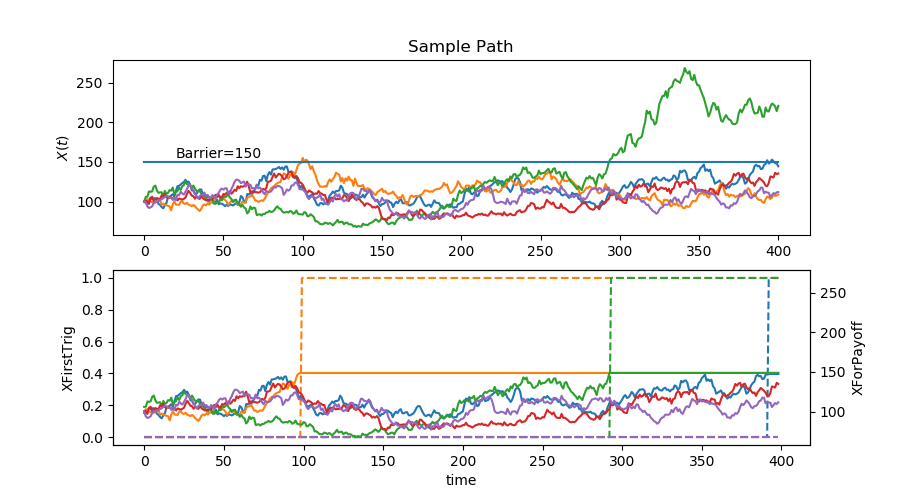
Figure 3 shows the values of these barrier breach tracking variables for a case with 400 time steps, and an upper barrier at level 150, for the same parameters of the dynamics as defined in Table 2, in the next section. The upper panel shows while the lower panel shows (scale on left axis) and (scale on the right axis). The solid lines show several realizations of corresponding to the same colored realization of in the upper panel. One can see that stays at the barrier level (“has been stopped”) once the barrier has been touched (for the orange path short before time step 100, for the green path short before time step 300). If the barrier is never touched, is just . Correspondingly, the dashed lines reflect - the orange line jumps to 1.0 (true) when the orange path touches the barrier short before time step 100, the green line jumps to 1.0 (true) short before time step 300, and none of the other lines jump. In the case with several barriers or more complicated barrier domains and conditions, and would identify the time and place the barrier was hit and thereby identify the barrier.
6 Results
We present the results of the forward deep BSDE barrier pricer for an Up-and-Out call option with a single underlier, with the parameters of the dynamics and the instrument as shown in Table 2, along with initial value for sample paths, , chosen uniformly within 50 and 150. We use the generator for the risk-neutral (discounting-only) case, as shown in section 2. However, any generator such as a generator for differential rates or other nonlinear pricing settings could be easily used instead.
The hyper-parameters of the computational graph and the embedded neural networks include (a) The number of time steps in the discretization, (b) The number () of layers for each for and the network; and (c) The number of units per layer (). The number of layers () and units per layer () for both the network and the networks are for the hidden layers. The input layer will always have as many units as the dimension of the problem, the output layer for the networks will be the same size as the input layer, and the output layer for the network will only have one unit. We also tested different mini-batch sizes (sample paths per mini-batch, ) for 20,000 mini-batch steps. The results are summarized in Table 3. The loss function value after those 20,000 mini-batch steps depends on the network configuration and the number of discretization time-steps. Among the several good hyper-parameters from the Table, the configuration with ( , ,with 200 time steps) was used for subsequent tests.
| (Barrier Position) | (Strike) | |||
|---|---|---|---|---|
| 0.2 | 0.05 | 0.5 Years | 150.0 | 100.0 |
| Loss function values after 20,000 mini-batch steps | ||||||||||
|---|---|---|---|---|---|---|---|---|---|---|
| Hyper Parameters | time steps = 50 | time steps = 100 | time steps = 200 | |||||||
| b=256 | b=512 | b=1024 | b=256 | b=512 | b=1024 | b=256 | b=512 | b=1024 | ||
| n=3 | u=3 | 21.09 | 19.04 | 15.71 | 19.43 | 14.38 | 21.35 | 23.45 | 19.45 | 22.43 |
| u=5 | 12.46 | 17.01 | 11.82 | 10.65 | 13.67 | 8.79 | 12.5 | 12.86 | 12.64 | |
| n=5 | u=3 | 11.32 | 9.89 | 8.99 | 8.9 | 11.49 | 10.2 | 12.09 | 9.35 | 8.75 |
| u=5 | 11.86 | 7.5 | 12.19 | 8.52 | 8.78 | 7.6 | 8.93 | 7.87 | 6.4 | |
| n=7 | u=3 | 17.45 | 13.07 | 16.93 | 27.06 | 29.55 | 23.79 | 35.19 | 21.99 | 40.46 |
| u=5 | 9.59 | 13.37 | 29.14 | 16.63 | 31.26 | 23.43 | 26.31 | 17.08 | 27.44 | |
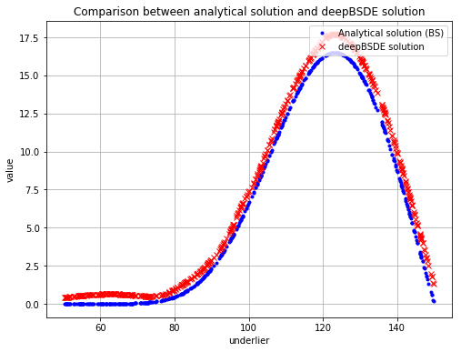
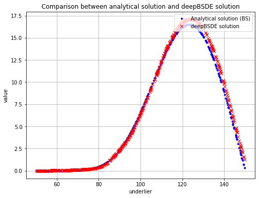
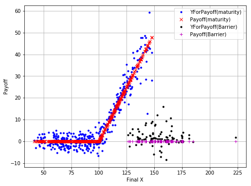
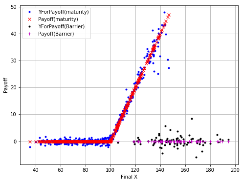
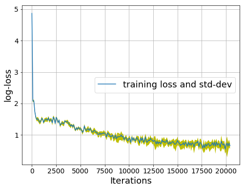
The price of option at time 0, as learned by the initial network is compared to the analytic solution of the time-continuous problem in Figure 4, is seen to be in close agreement and is better approximated with larger number of training mini-batches. The results show this methodology is successful in replicating the appropriate payoff as shown in Figures 4(c) and 4(d). The payoff approximation is shown for sample paths that have not breached the barrier (blue) as well as those that have knocked out (black). The loss (measured as the MSE of difference between and payoff) as computed from the mini-batch and its standard deviation are shown in Figure 5(a), and the loss is seen to definitely decrease with larger number of iterations.
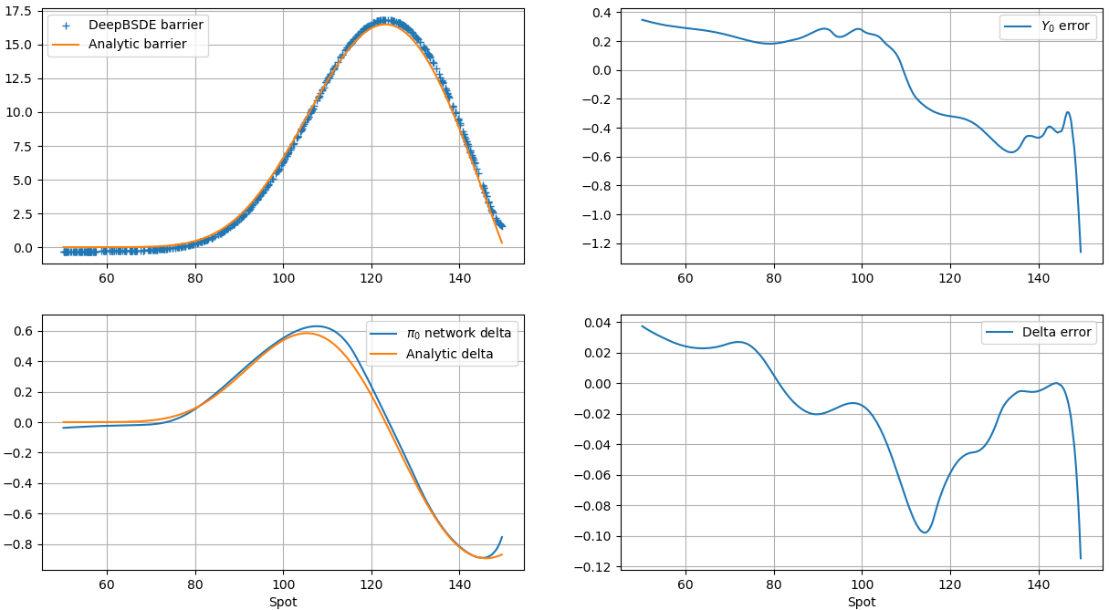
Furthermore, another neural network design with batch normalization and 5 hidden layers with 7 units per layer was trained and results are shown in Figure 7. As mentioned earlies, for the time-continuous case and exact solution of the minimization problem, would be and would represent the delta at time 0. Thus, it is compared to the analytical delta of the option as given by the known closed-form solution. The differences between the analytical and learned values is shown on the plots on the right of the panel. As also discussed earlier, one would not expect arbitrarily close agreement between analytical and learned values for the time-discrete case.
6.1 Hedging PnLs
As discussed earlier, the networks give how many units of each underlier are in the trading strategy and that trading strategy for the time-continous case and appropriate risk measures such as error would be the delta-hedging strategy corresponding to a given analytical solution . It is standard to implement time-discrete delta-hedging trading strategies that adjust the portfolio to units of underliers at given discrete time instances .
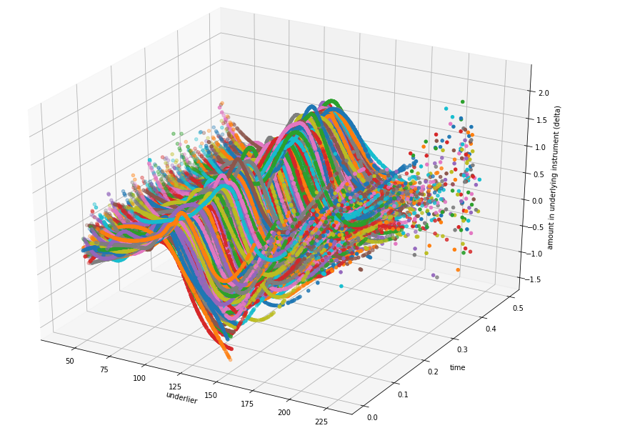
The position in the portfolio for the underlier (corresponding to Delta) as learned by the networks is shown in Figure 5(b), as a function of the time and the underlier as a 3D plot.
The difference between value of the trading strategy at maturity or barrier and the payoff specified by the instrument can be understood as hedging PnL resulting from such hedging at discrete times. This hedging PnL as obtained from the deep BSDE solution at different number of mini-batches during the training is shown in Figure 6. Since the hedging is only performed at discrete times, it is expected to deviate from theoretical PnL of zero for continuous hedging. One can see that as the training proceeds on more and more mini-batches, the hedging PnL is more strongly peaked at 0 and has fewer outliers.
It is also interesting to compare the trading strategy obtained from the deepBSDE method to the trading strategy implied by delta-hedging according to the known analytical solution for barrier problem in the time-continuous case (which is obtained by setting to the analytical gradient of the known analytical solution evaluated at time ).
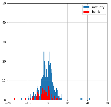
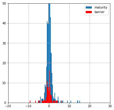
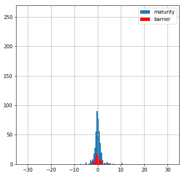
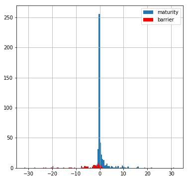
The histogram of the hedging PnL (final value of strategy versus required payoff) for the hedging strategy from the trained network is shown in Figure 8(a), for both the active as well as the knocked-out case. In contrast, the hedging PnL obtained by using the analytical value of the Option Deltas is shown in Figure 8(b).
It can be seen that the hedging by analytical Option Deltas yields small PnL in a majority of cases, however performs poorly for a number of cases where PnL assumes a large relative value (-30 to 30) due to imperfections in discrete-time hedging. In contrast, the Deep Learning based approach yields very small PnL in comparitively smaller number of cases, has better overall risk performance (and generally small PnL) and smaller extreme errors/performance compared to the hedging with analytic Delta.
7 Acknowledgement
The authors would like to thank Fernando Cela Diaz and Pallavi Abhang for their help on setting up and running large scale hyper-parameter optimization on distributed computing infrastructure, Orcan Ogetbil for discussions on barrier option pricing, Vijayan Nair for discussion regarding methods, presentation, and results and Agus Sudjianto for supporting this research.
8 Conclusion
We proposed a novel deep neural network based architecture to price Barrier Options via Deep BSDE, that captures whether the underliers’ price movement touched the barrier or not in order to model the appropriate payoff conditions and minimize the payoff error in order to learn the price of the option at initial time. We also demostrated the effectiveness of the hedging strategy via Deep BSDE learned Deltas at discrete time instances.
References
- [CWNMW19] Quentin Chan-Wai-Nam, Joseph Mikael, and Xavier Warin. Machine learning for semi linear PDEs. Journal of Scientific Computing, 79(3):1667–1712, 2019. arXiv:1809.07609.
- [EKPQ97] Nicole El Karoui, Shige Peng, and Marie Claire Quenez. Backward stochastic differential equations in finance. Mathematical finance, 7(1):1–71, 1997. Also available on semanticscholar.org.
- [Hie19] Bernhard Hientzsch. Introduction to solving quant finance problems with time-stepped FBSDE and deep learning. arXiv preprint arXiv:1911.12231, Nov 2019. Also available at SSRN: https://ssrn.com/abstract=3494359 or http://dx.doi.org/10.2139/ssrn.3494359.
- [HJE18] Jiequn Han, Arnulf Jentzen, and Weinan E. Solving high-dimensional partial differential equations using deep learning. Proceedings of the National Academy of Sciences, 115(34):8505–8510, 2018.
- [Mer15] Fabio Mercurio. Bergman, Piterbarg, and beyond: pricing derivatives under collateralization and differential rates. In Actuarial Sciences and Quantitative Finance, pages 65–95. Springer, 2015. Also available at SSRN: https://ssrn.com/abstract=2326581 or http://dx.doi.org/10.2139/ssrn.2326581.
- [Per10] Nicolas Perkowski. Backward Stochastic Differential Equations: an Introduction, 2010. Available on semanticscholar.org.
- [Rai18] Maziar Raissi. Forward-backward stochastic neural networks: Deep learning of high-dimensional partial differential equations. arXiv preprint arXiv:1804.07010, 2018.
- [Shr04] Steven Shreve. Stochastic Calculus for Finance II. Springer-Verlag New York, 2004.
- [YXS19] Bing Yu, Xiaojing Xing, and Agus Sudjianto. Deep-learning based numerical BSDE method for Barrier options. arXiv preprint arXiv:1904.05921, 2019. Also available at SSRN: https://ssrn.com/abstract=3366314 or http://dx.doi.org/10.2139/ssrn.3366314.