A machine learning approach to using Quality-of-Life patient scores in guiding prostate radiation therapy dosing

Abstract

Thanks to advancements in diagnosis and treatment, prostate cancer patients have high long-term survival rates. Currently, an important goal is to preserve quality-of-life during and after treatment. The relationship between the radiation a patient receives and the subsequent side effects he experiences is complex and difficult to model or predict. Here, we use machine learning algorithms and statistical models to explore the connection between radiation treatment and post-treatment gastro-urinary function. Since only a limited number of patient datasets are currently available, we used image flipping and curvature-based interpolation methods to generate more data in order to leverage transfer learning. Using interpolated and augmented data, we trained a convolutional autoencoder network to obtain near-optimal starting points for the weights. A convolutional neural network then analyzed the relationship between patient-reported quality-of-life and radiation. We also used analysis of variance and logistic regression to explore organ sensitivity to radiation and develop dosage thresholds for each organ region. Our findings show no connection between the bladder and quality-of-life scores. However, we found a connection between radiation applied to posterior and anterior rectal regions to changes in quality-of-life. Finally, we estimated radiation therapy dosage thresholds for each organ. Our analysis connects machine learning methods with organ sensitivity, thus providing a framework for informing cancer patient care using patient reported quality-of-life metrics.

1 Introduction

Approximately 175 thousand new cases of prostate cancer were reported in 2019 in the United States [18]. Depending on age and cancer stage, first-line treatments include prostatectomy, radiation treatment, and androgen ablation. Each of these treatments carries different side effects. For some patients, a prostatectomy is followed by radiation treatment to minimize the possibility of recurrence. Radiation planning for each patient begins with a CT scan, which is followed by the demarcation of the prostate (radiation target) and the surrounding organs (bladder and rectum) by a physician. Each plan is customized to a patient as there is some flexibility in the spatial dosing of radiation with the primary consideration being delivery of sufficient dosage of radiation to the target organ without overexposing and damaging surrounding organs and structures. Radiation treatment (RT) plans are developed using Dose Volume Histograms (DVH). DVH discard all organ-specific spatial information and they are usually based on a single planning CT scan that does not account for anatomical variations over the course of several weeks of therapy [10]. Various metrics have been developed in order to translate the information from a DVH into a computed probability of uncomplicated tumor control using normal tissue complication probability models (NTCP) [10]. These efforts are necessary as the relationship between exposure to radiation of the surrounding organs/structures and the severity and probability of toxicity (urinary and bowel) is still not fully understood. From a physiological perspective, it is not clear how radiation dosage affects tissues, organs, as well as their control and function.

In order to develop a radiation plan that minimizes patient side effects, one needs to quantify these side effects post-radiation. Traditionally, physician-assessed scoring systems have been widely used for measuring patient side effects following cancer treatment [3]. However, more recent evidence indicates that clinicians can downgrade the frequency and severity of patients’ treatment-related symptoms [3, 14]. Patient-reported health-related quality-of-life (QOL) surveys are becoming an important tool in measuring outcomes after cancer treatment [17, 20]. For example, a study by K. Diao et al. [4] explored urinary and bowel symptom development during treatment using patient-reported QOL scores (from 1, indicating no symptoms, to 5, indicating high frequency of symptoms). An IRB waiver was received at the University of North Carolina for this retrospective study using anonymized data. The results showed that average scores progressively increased from baseline throughout treatment, but all symptoms resolved to baseline levels by follow-up. In the context of RT, NTCP models can be correlated to patient-reported QOL data, as was done in [11]. However their analysis focused only on urinary symptoms during post-prostatectomy radiotherapy and NTCP models rely on already reduced DVH information. Given the rich organ-specific information obtained during treatment planning, it could be desirable to more directly connect 3D patient CT scans and dosing with QOL scores.

Machine learning methods have become state of the art in many applications with impressive results; deep convolutional networks have many times outperformed traditional methods for diagnosis [15] or visual recognition tools [8]. In biomedical imaging, deep convolutional neural network (CNN) algorithms have been applied to a wide array of problems. Of particular interest in our context are medical image segmentation machine learning algorithms, such as the U-net [16] architecture that focuses on semantic segmentation of biomedical images. The U-net architecture has appealing features that we will employ in our approach such as it uses a large number of max-pooling operations to allow for the identification of global, non-local features and up-convolution to return images to their original size. In the work of Nguyen et al. [13], a modified U-net architecture was shown to accurately predict voxel-level dose distributions for intensity-modulated radiation therapy for prostate cancer patients. These prior studies indicate tremendous promise of guidance of radiation treatment planning with artificial intelligence-based algorithms. Nevertheless, these algorithms can be of significant use in treatment planning if they can also incorporate QOL predictions that can provide immediate guidance for the dosimetrist during clinical plan optimization. To our knowledge, there are no prior approaches that integrate QOL in machine learning algorithms in the context of RT for prostate cancer.

In the department of Radiation Oncology at the University of North Carolina, QOL scores were collected using a validated questionnaire [19] administered during weekly treatment visits as part of the routine clinical work-flow for prostate cancer patients. While QOL data have been studied post prostate cancer radiation treatment, data collected during the course of treatment can convey important information about symptom development, which can be a fertile ground for the use of quantitative modeling to guide optimal RT dosing. Accordingly, in this paper we analyze data from a 14-question quality-of-life prostate cancer patient survey that was collected over the span of five years (2010-2015). The data we examined tracked patient urinary and bowel side effects before and along the course of their treatment (about seven weeks). Associated with each patient’s QOL, we also examined associated anatomical CT scans and radiation dosing patterns for approximately 50 patients.

In this paper, we propose a CNN algorithm to explore the connection between the spatial distribution of the RT dose and the QOL outcomes reported from patients in our data set. A significant problem with CNN algorithms in our context is the need for a sufficiently large data set; to resolve this issue, we augmented our patient data sets using interpolation algorithms that generated synthetic patients by combining existing patient data. In addition, we used transfer learning in order to improve the performance of our CNN algorithm and implemented steps to avoid overfitting the problem. A key goal for our study was to generate insight into the most radiation-sensitive tissue regions.

As a comparative alternative to the CNN approach, we also used analysis of variance and logistic regression to explore organ sensitivity to radiation and develop dosage thresholds for each organ region. We identified regions of the rectum that were highly correlated with changes in individual patient symptoms. Finally, we estimated radiation therapy dosage thresholds to determine how high radiation therapy dosage needed to be in order to trigger collateral symptoms. Combining results from machine learning and direct analyses of organ sensitivity provides a powerful framework to inform patient care in the quality-of-life context.

This paper is organized as follows. In the Methods section, we formulate convolutional neural network algorithms and statistical models. In the Results section, we demonstrate that the CNN algorithm we developed can identify correlations between bowel-related symptoms and radiation. Furthermore, we support these findings through statistical analyses that explore organ sensitivity to radiation dosage. Finally, in the Discussion and Conclusions section, we compare our results with those of previous studies.

2 Methods

2.1 Quality-of-life data

Our patient-reported data were extracted from a patient quality-of-life survey containing answers to 14 questions, seven questions pertaining to urinary symptoms and seven concerned with bowel symptoms. The specific survey questions and possible responses are shown in Appendix A. Patients took the survey before undergoing radiation therapy, once a week during the seven-week-long treatment, and after completing therapy. Answers by patient $j$ to question $i$ at time point $t=\{0,1,2,3,4,5,6,7\}$, $a_{ij}(t)$, were scored on a discrete scale ranging from 1 to 5 (a score of 1 indicating the least severity in symptoms, and a score of 5 indicating very high severity in symptoms). We used this quality-of-life survey and de-identified CT scans and treatment plans for a total of 52 patients (note that 57 patients were provided, however, five patients had incomplete data and were discarded in our analysis).

The answers $a_{ij}(t=0)$ to the first survey taken before treatment were used as the baseline of symptoms before radiation therapy. Subsequent answers $a_{ij}(t\geq 1)$ provide information on patient $j$’s symptoms associated with question $i$. In order to reduce the dimensionality of the data set collected over several weeks, we developed a single score for urinary-related symptoms and bowel-related symptoms as follows.

For each patient, we divided the questions and associated answers into those concerning urinary or bowel function and then identified the worst (maximum) score $a^{*}_{ij}\equiv{\rm max}_{t}a_{ij}(t)$ a patient reported throughout the multi-week treatment for each question. A single total difference score for each patient $j$, $\Delta_{j}$, was computed as the difference $a_{ij}^{*}-a_{ij}(0)$, summed over the urinary- or bowel-subset of answers $i$:

$$\Delta_{j}^{\rm u}=\sum_{i=1}^{7}\left[a^{*}_{ij}-a_{ij}(0)\right],\quad\Delta_{j}^{\rm b}=\sum_{i=8}^{14}\left[a^{*}_{ij}-a_{ij}(0)\right].$$ (1)

Here, we have ordered questions and corresponding answers associated with urinary function as $i=\{1,2,3,4,5,6,7\}$ and the bowel-associated questions as $i=\{8,9,10,11,12,13,14\}$. The total difference score $\Delta_{j}^{\rm u}$ and $\Delta_{j}^{\rm b}$ represent the total change in the quality of life associated with urinary and bowel function, respectively.

Next, we used a cut-off (or threshold) value of 6 to convert the patient’s quality-of-life responses into a binary classifier defined by the discrete Heaviside function

$$y_{j}\equiv H(\Delta_{j}-6)=\begin{cases}0&\Delta_{j}<6,\\ 1&\Delta_{j}\geq 6.\end{cases}$$ (2)

Score thresholding can be visualized in Figure 1 that shows the urinary total difference scores for each patient overlaid with colored boxes that mark the score cut-off value. The threshold of 6 was initially arbitrarily chosen using the fact that it is more than half of greatest sum of changes for patients; however, we tested other thresholds in order to discern issues with the binary classifier as detailed in the Results section.

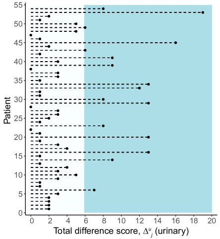
Figure 1: Total difference scores in urinary symptoms for patients 1-54. In blue, we mark patients who were classified as having a significant change in symptoms with $\Delta_{j}^{\rm u}\geq 6$.

2.2 Image augmentation

Previous biomedical studies focusing on image processing have used data sets as small as 85 data points [7] and as large as 100,000 data points [15]. Since the amount of data points we have is even smaller than 85, we decided to enrich our dataset prior to training our algorithms. We used the Fischer-Modersitzki (FM) curvature-based image registration technique [5] in order to generate new in silico patients as interpolations of existing patient data.

The FM approach was developed in the context of image registration. For completeness, we outline the core ideas of image registration algorithms here. Let $d$-dimensional images be represented by compactly supported mappings $T,R:\Omega\to\mathbb{R}$ where $\Omega=]0,1[^{d}$. Specifically, the quantity $T({\bf x})$ is the intensity or image grey value at the spatial position ${\bf x}\in\Omega$. Given a reference image $R({\bf x})$ and a deformable template image $T({\bf x})$, a registration algorithm outputs a deformation, or displacement field, ${\bf u}:\mathbb{R}^{d}\to\mathbb{R}^{d}$ such that when applied to the template image, $T({\bf x}-{\bf u}({\bf x}))$ a resulting modified template more closely matches the reference, $R({\bf x})$. The problem is then how to find a desired deformation ${\bf u}=(u_{1},\ldots,u_{d})$. This becomes an optimization problem as one tries to minimize the difference between the deformed template $T_{{\bf u}}\coloneqq T({\bf x}-{\bf u}({\bf x}))$ and the reference $R({\bf x})$.

Variations in registration methods arise when one employs a particular optimization technique and one must define a metric for measuring the goodness of a deformation. Let $D$ be the distance measure between the reference $R$ and deformed template $T$, and $S$ a measure of the smoothness of the deformation ${\bf u}$. The FM approach consists of finding ${\bf u}$ by minimizing the joint functional $J[{\bf u}]$,

$$J[{\bf u}]\coloneqq D[R,T;{\bf u}]+\alpha S[{\bf u}].$$ (3)

The regularization parameter $\alpha$ is used to control the strength of the smoothness of the displacement versus the similarity of the images. The difference-squared measure $D$ is given by

$$D[R,T;{\bf u}]\coloneqq{1\over 2}\|R-T_{{\bf u}}\|^{2}={1\over 2}\int\limits_{\Omega}(R({\bf x})-T({\bf x}-{\bf u}({\bf x})))^{2}{\rm d}{\bf x},$$ (4)

and the curvature-based smoothness

$$S[{\bf u}]\coloneqq{1\over 2}\sum_{j=1}^{d}\int\limits_{\Omega}(\Delta u_{j})^{2}{\rm d}{\bf x},$$ (5)

with Neumann boundary conditions defined by

$$\nabla u_{j}({\bf x})=0,\quad{\bf x}\in\partial\Omega,\quad j=1,\ldots,d.$$ (6)

We obtain a minimizer $\mathbf{u}$ by first ensuring that the Gâteaux derivative of the objective function vanishes. The resulting Euler-Lagrange equations are

$$f({\bf x},{\bf u}({\bf x}))+\alpha A[{\bf u}]({\bf x})=0,\quad{\bf x}\in\Omega.$$ (7)

with

$$f({\bf x},{\bf u}({\bf x})) =(R-T_{\bf u})\cdot\nabla T_{\bf u}({\bf x})=(R({\bf x})-T({\bf x}-{\bf u}({\bf x})))\cdot\nabla T({\bf x}-{\bf u}({\bf x})),$$ (8)

$$A[{\bf u}]({\bf x}) =\Delta^{2}{\bf u}.$$ (9)

The above semi-linear partial differential equations (PDE) are known as the Navier-Lame biharmonic and diffusion equations.

The Euler-Lagrange PDE’s can be solved using the following fixed-point iteration

$$\alpha A[{\bf u}^{k+1}]({\bf x},t) =-f({\bf x},{\bf u}^{k}({\bf x},t)),\quad k\geq 0,$$ (10)

$${\bf u}^{0} =0.$$ (11)

Since the computational domain $\Omega$ is of a simple geometry in this case, a finite difference approximation for the derivatives can be used. This yields a linear system of equations that are solved in each iteration step to obtain the deformation ${\bf u}$; more details of the discretization scheme we implemented to solve for ${\bf u}$ are given in [5].

Returning to our problem, the goal is to take each CT slice of patient A and interpolate it with each CT slice of patient B creating a new stack of CT image slices for a new “patient” C. We achieved this interpolation by applying the FM registration approach and selecting one stack of images to serve as the reference and another to serve as the template. We implemented FM in Matlab, using the discretization approach outlined above and also the implementation outlined in [9]. A new interpolated patient C was obtained by applying the deformation to the template CT image stacks. We performed this procedure on the 52 patients’ cropped CT image stacks for the bladder and the rectum respectively, thus producing 1,326 new images for each organ. An example of the interpolated CT images we obtained using this method is shown in Figure 2.

(a) Reference

(b) Template

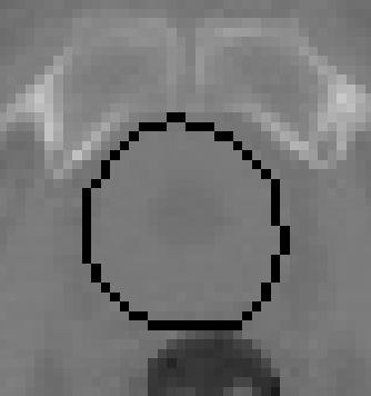
(c) Interpolation

Figure 2: Interpolation of CT images of the bladder using the FM algorithm. The interpolated image (c) is the deformed version of the template image (b) against the reference image (a).

2.3 Radiation Plans

Radiation plans are overlayed on a baseline CT scan and they give the spatial distribution of the doses that will be given to a patient over the course of treatment. When the plan is mapped onto a CT image, high radiation dosage regions are denoted by high pixel intensity (white) while low dosages are represented by darker pixels. A cross-section of a representative radiation plan is shown in Figure 3. We applied FM interpolation onto the radiation plan images for each in silico patient. Specifically, we interpolate between radiation plans of patient A and patient B to create a new stack of radiation plans for a new “patient” C.

Figure 3: A representative radiation plan. The highest dosage corresponds to the greatest pixel intensity (in white). Black pixels correspond to no radiation.

2.4 Convolutional neural network model

Next, we constructed a 3-level 3D convolutional neural network (CNN) model for each organ: one processing data related to urinary symptoms and one processing data related to rectal symptoms. The architecture of the model is illustrated in Figure 4.

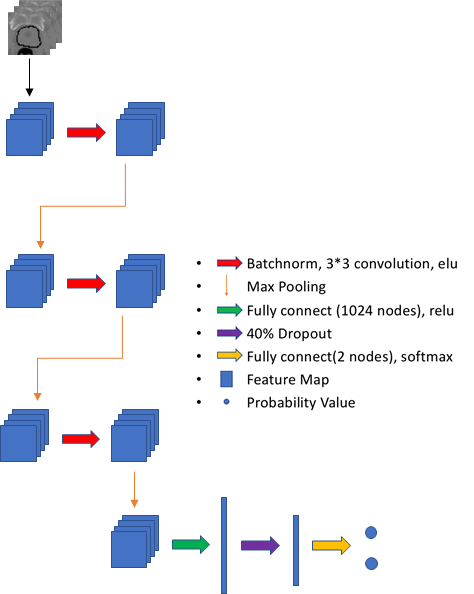
Figure 4: Architecture used for the CNN classification model. There are three layers that have convolution, activation, and pooling. The last convolution layer is connected by fully connected layers and a drop-out layer which drops out 40% information to avoid over-fitting. Finally the model output two nodes which tell the predicted probability that a patient will or will not manifest change in (urinary or bowel) symptoms throughout treatment

The convolutional layers use filters of size $3\times 3\times 3$ and strides of 1. Each of the 3 convolutional layers is followed by max pooling, which reduced the feature size from $48\times 48$ pixels down to 1 pixel. We chose to use max pooling for our pooling method so that the filters captured the strongest (and thus highest) pixel value for each stride (we use strides of 1 for each filter and a pooling size of [2,2,2]). In addition, each convolutional layer is followed by an exponential linear unit (ELU) activation function defined as

$$f(x)=\begin{cases}e^{x}-1&x<0,\\ x&x\geq 0.\end{cases}$$ (12)

We used batch normalization (BN) after the convolution and ELU operations, which have been shown to update weights equally throughout the CNN, resulting in faster convergence [12]. In addition, we used drop-out (40 percent rate) to reduce overfitting since our dataset was small. Because our model is a classifier, we use a cross-entropy loss function that the network minimizes through back-propagation:

$${\rm Loss}(k)=-\frac{1}{N}\sum_{j=1}^{N}y_{j}\log p_{k}(y_{j})+(1-y_{j})\log(1-p_{k}(y_{j})),$$ (13)

where $k$ is the step number, $y_{j}=\{0,1\}$ classifier label of the $j^{\rm th}$ patient, and $p_{k}(y_{j})$ represents the predicted probability for the corresponding label at the $k^{\rm th}$ iteration.

Our CNN had 2 channels as part of its input layer: one to process information related to the patient CT scans, and one to process information related to the patient RT plans. The input data consisted of 52 patient CT scan stacks and RT plans cropped around the organ of interest (either the bladder or the rectum) with the respective organ doctor annotated contours for each CT scan. The CT scans and RT plans were cropped because the information outside of the organs of interest was not useful for the purposes of this study. Cropping also minimized the computational power needed to run our algorithm. The final layer of the model consisted of two nodes: one providing the predicted probability that a patient would manifest a change in (urinary or bowel) symptoms throughout treatment; and one giving the predicted probability that a patient would not manifest a change in (urinary or bowel) symptoms throughout treatment. In addition, the CNN produced a confusion matrix (for either the urinary or bowel symptoms) outlining how many patients it accurately predicted from the testing set.

To assess the overall performance of our model, the CNN trained on 39 patients with a batch size of 20 and learning rate of 0.001 for approximately 12 hours, and was then tested against the remaining 13 patients. Patients were shuffled and randomly assigned to the training and testing sets to avoid bias. The CNN also employed a 5-fold cross-validation procedure on the training set, similar to the approach in Jiang et al. [6]. Each of the 5 folds split the training set into 31 training patients and 8 validation patients, respectively. Every fold initialized a classifier (for a total of 5 classifiers), from which we could select the model that performed best, based on its accuracy and number of true-positives, and evaluated it on the testing set. We used the number of true-positives as a criterion for the best-performing model in order to avoid only predicting a lack of a change in symptoms. The cross-validation model and corresponding loss functions used can be visualized in Figure 5.

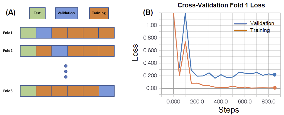
Figure 5: (A) Model cross-validation. We initialized 5 different models. For each model there is a validation set that moves across the data. First, we trained on the training set, then checked each of the models on the different validation sets, providing a general idea of which model would work the best. (B) Training (orange) and validation (blue) loss for the best model chosen through cross-validation. As shown in orange, the training loss becomes very small, but the validation loss stays at about $0.2$.

2.5 Autoencoder

We employed a convolutional autoencoder network that uses a portion of the CNN architecture. Specifically, instead of connecting to a fully connected layer after all the convolution layers as we did with the CNN, the autoencoder was used to pre-train the network on unlabeled information by reconstructing the original images. The convolutional autoencoder network architecture is illustrated in Figure 6 and is similar to the U-net architecture used in related segmentation problems [7, 2]. After the autoencoder was trained, we truncated the network at the start of the deconvolution layers and connected it to a fully connected layer that served as the output for our new CNN model.

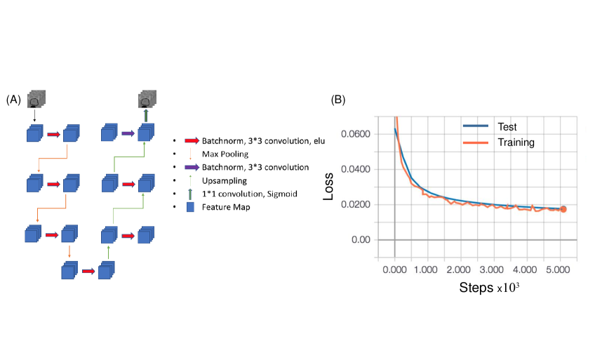
Figure 6: Convolutional Autoencoder. (A) Schematic of the architecture of the convolutional autoencoder network. Three layers have convolution, activation, and pooling. The network deconvolves with activation and pooling for three more layers. The network targets to reconstruct the input image with the goal to learn the key features of the CT scans and RT plans. (B) Autoencoder loss while training on the bladder data. The blue curve shows the loss for the test set and the orange curve shows the loss for the training set. Both decrease with the number of iterations of the autoencoder.

Training of the autoencoder allowed us to implement a transfer learning approach where we first trained the autoencoder network to reconstruct patient images and assigned the near-optimal weights obtained from autoencoder training as initial conditions for the CNN network with the binary classifier. This pre-training was necessary due to the small size of of the dataset.

2.6 Statistical analysis for dose thresholding

In order to further explore the relationship between QOL scores and RT dosage, we investigated whether or not there were any correlations between a certain organ region’s RT dosage and whether or not the patient experienced a change in symptoms related to that organ. We accomplished this through the use of analysis of variance (ANOVA) and logistic regression.

We first built an algorithm to obtain the RT dosage on the rectum and bladder contours. We fed the cropped image of the organ of interest (with overlaid contours from the earlier data preparation process) into the algorithm and obtained a new image of the organ with thicker contours. The algorithm was able to do this by locating the center of the organ and obtaining a radius that traces around the organ’s original (doctor annotated) contour to obtain the new, thicker contour. This allowed us to obtain more information on the RT dosage located around the contour of the organ. We were then able to obtain the RT dosage corresponding to the area occupied by the new, thicker organ contours. Had we used the original organ contours, we may not have had the most complete information on the prescribed amount of RT. The new, thick bladder contours with the corresponding RT dosage are shown in Figure 7.

Following this procedure, we combined all CT images of one patient into a three dimensional cube and separated it into either top and bottom, or front and back regions. We split the bladder into top and bottom halves and the rectum into front and back regions using the following rationale. Since the bottom of the bladder is closer to the prostate, we speculated this region would be exposed to more radiation and thus be associated with a higher incidence of collateral urinary symptoms. Therefore, we split the bladder into top and bottom. As for the rectum, we split it between front and back, since the front is closer to the prostate and we thus anticipated it would be exposed to a higher radiation dosage. Organ regions are illustrated in Figure 7(C).

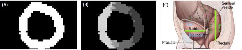
Figure 7: Organ contouring and organ regions. (A) A CT slice of the rectum of patient 40, showing the new thick contour. (B) Same as (A) but showing the thick contour with the corresponding RT dosage. (C) Lateral view diagram showing how the bladder (yellow) and rectum (red) were split for spatial RT analyses. Image from http://libcat.org/anatomy-of-prostate-cancer.

Finally, we define a quantity $d_{lj}$ as the total RT dosage measured in cGy for a specified organ region, $l$ and patient, $j$. Total dosages were computed for: ($l=1$) top of the bladder, ($l=2$) bottom of the bladder, ($l=3$) total bladder, ($l=4$) front of the rectum, ($l=5$) back of the rectum, and ($l=6$) total rectum.

Organ sensitivity. We first conducted a paired 2-tailed t-test to evaluate whether or not the total average dosages were significantly different across all the regions outlined above. We found that all regions had significantly different total RT dosages ($p<0.05$), which further prompted us to investigate whether or not these differences in RT dosage had an impact on patients’ QOL scores throughout treatment. To accomplish this, we converted the QOL survey scores into a binary classifier per question as follows

$$y^{d}_{ij}\equiv H((a^{*}_{ij}-a_{ij}(0))-2)=\begin{cases}0&a^{*}_{ij}-a_{ij}(0)<2,\\ 1&a^{*}_{ij}-a_{ij}(0)\geq 2.\end{cases}$$ (14)

Using this approach, we obtained a binary value $y^{d}_{ij}$ for each survey question $i$ and patient $j$ so that we could identify which symptoms were significantly affected by the corresponding RT dosage. Then, the binary data were used in one-way ANOVA, which compared the distribution of RT dosage for a given organ region ($l=1,\dots,6$) between the two patient groups ($y^{d}_{ij}=1$ vs $y^{d}_{ij}=0$) for a given symptom question $i$. Recall that using our convention urinary questions, $i=1-7$ correspond to regions $l=1-3$ and bowel-associated questions, $i=8-14$ correspond to regions $l=4-6$. This analysis allowed us to identify which specific symptoms were significantly affected by the corresponding RT dosage for a given organ region.

Dosage Thresholding. Since the previous analysis identified organ regions that were associated with significant changes in symptoms, we next investigated the ranges of RT dosage that could trigger such changes. We used logistic regression applied to all the original binary patient classifiers $y_{j}$ (from Eq. (2)) and region total doses, $d_{lj}$ in order to predict whether a patient would experience changes in symptoms given the corresponding region dose, $d_{lj}$. The goal of this analysis was to identify the lowest RT dose for patients with changes in symptoms ($y_{j}=1$) and the highest RT dose for patients that did not have a change in symptoms ($y_{j}=0$).

For each logistic model, a tunable RT dose threshold parameter, $\theta$ determined to which category patients were assigned based on the model’s prediction, $\hat{y}_{j}$. For each region $l$, we varied $\theta$ until we obtained a $\theta_{p}$ corresponding to no false positives and a $\theta_{n}$ corresponding to no false negatives when comparing $y_{j}$ with the predicted logistic classifier $\hat{y}_{j}$. Once we obtained the thresholding parameters for each region, $l$, we recorded the corresponding RT dosage ranges and used them to infer how high RT dosage had to be in order to trigger collateral symptoms.

3 Results and Discussion

3.1 CNN results

We evaluated the performance of the CNN network using a measure of accuracy defined to be the number of patients with correctly predicted outcomes over the total number of patients. We estimated accuracy results for the bladder and the rectum symptoms by running our algorithm 10 times and averaging the results. We did not find conclusive results for the bladder, as we obtained an average accuracy of 38% with a range of 23% to 53%. This indicated that the CNN model, using the available data, did not find any patterns to classify the patients for bladder symptoms. For the patients with a change in bladder symptoms, there was a lot of variability in model predictions ranging anywhere from 0% to 50% with an average of 27%.

In contrast, promising results were obtained for classification of rectal symptoms. Our model with cross-validation accurately predicted an average of 74% changes in rectal symptoms with a range of 62% to 84.5%. The results are visualized in Figure 8. For patients with a change in symptoms, the model was on average accurately predicting the change in symptoms 56% of the time with a range from 25% to 100%. In Table 1, we give the confusion matrix for the rectum model with the validation set that resulted in an 84.6% accuracy. Of the 10 patients without a change in symptoms, 9 of them were accurately predicted. Of the 3 patients with a change in symptoms, 2 were accurately predicted. The result is promising because the model is not always predicting one of the classes; it is picking up some patterns from the patients’ data so that it can classify the patients in either category.

We will show later that our results are rather insensitive to the threshold delineating quality-of-life changes.

Confusion Matrix (Rectum Symptoms)
Actual	Predicted
	No Change	Change
No Change	9	1
Change	1	2

Table 1: Confusion matrix for rectum model. Table shows the accuracy for one completely validated model. We show the actual classification of the patient, and what the model predicted.

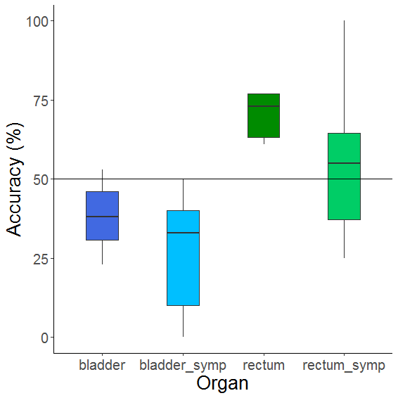
Figure 8: Accuracy for our trained classification model. The overall accuracy for the bladder and rectum and the model accuracy within patients who experienced symptoms (denoted with symp). As we can see with the bladder and bladder symptom accuracy, there were no significant differences, as results sit below the 50% line. For the rectum, the overall accuracy for predicting rectum symptoms exceed the 50% line.

3.2 Outcome thresholding

Other than classifying patients based on their quality-of-life score with a cut-off value of 6, we also used thresholds of 5 and 7 and used the reclassified data to train the classification model. Unsurprisingly, the accuracy rates are similar to those found using a threshold of 6.

For the data reclassified with a threshold of 5, our model with cross-validation accurately predicted an average of 69% changes in rectal symptoms.

For the data reclassified with a threshold of 7, we found an average accuracy rate of 69%. As there are no considerable differences in results when we change the threshold, reinforcing that our original choice of a cut-off-value, the half of the greatest sum of changes, is a reasonable way to classify patients based on their quality-of-life scores.

3.3 Statistical analysis results

Based on our ANOVA analyses for the bladder data, it does not appear that there were any significant differences between the two patient groups in regards to average spatial RT dosing for the bottom and top of the bladder, as shown in Table 2.

ANOVA Dose Difference Results
QoL Question	P-Value (Bottom of Bladder)	P-Value (Top of Bladder)
1(Flow Easiness)	0.5331	0.0763
2 (Frequency at Night)	0.2405	0.8652
3 (General Frequency)	0.58571	0.687
4 (Pain)	0.6682	0.1895
5 (Urgency)	0.5272	0.094
6 (Control)	0.9656	0.1767
7 (Leak)	0.7949	0.8284
All Questions	0.6172	0.6667

Table 2: P-values corresponding to the ANOVA analysis of each urinary symptom and the average RT dosage in the top and bottom of the bladder. $*$ indicates $p<0.05$ which we interpret as statistically significant.

ANOVA Dose Difference Results
Question	P-Value (Front of Rectum)	P-Value (Back of Rectum)
1 (Diarrhea)	0.0018*	0.0002*
2 (Urgency)	0.0025*	0.0006*
3 (Pain)	0.0023*	0.0008*
4 (Bleeding)	0.6563	0.4142
5 (Cramping)	0.0545	0.0015*
6 (Pass Mucus)	0.0387*	0.0185*
7 (Nothing to Pass)	0.0541	0.0504
All Questions	0.0123*	0.0112*

Table 3: P-values corresponding to the ANOVA analysis of each rectal symptom and the average RT dosage in the front and back of the rectum. $*$ indicates $p<0.05$ which we interpret as statistically significant.

According to our ANOVA analyses on rectum data, those who experienced changes in symptoms of diarrhea, urgency, pain, and passing mucus had significantly higher average RT dosage in the front of the rectum. Furthermore, those who experienced changes across all rectal symptoms had a significantly higher average RT dosage in the front of the rectum. We found the same results for the back of the rectum (with a difference in cramping which turned out to be significant for the back but not the front). The corresponding p-values for both organ regions are listed in Table 3. The results indicate that the rectum is more sensitive to radiation therapy, matching the results from our CNN model.

According to our logistic threshold analysis, we found that patients tend to develop bowel-related symptoms throughout the treatment if they are receiving doses more than 2,500 cGy in the rectum. Correspondingly, in Figure 9(A), we also found that the safe doses to the rectum range from 1,250 to 2,950 cGy, implying that a dose greater than 2,950 cGy will trigger the development of collateral symptoms. If we further assume the radiation dosages to the different parts of the rectum are uncorrelated, we can also independently find dosage thresholds for the front and back of the rectum. We observed that the front of the rectum could tolerate a higher range of absolute dosage (2,100-4,300 cGy) than the back of the rectum (400-1,700 cGy). These threshold values are listed in Figure 9(A) and similar results for the top, bottom, and total bladder regions are shown in Appendix B.

While this conclusion is consistent with the correlation found between the rectal symptoms and rectum dosages in the interval 2500-4200 cGy [1], we cannot rule out that it could result from a possible collinear effect in which patients received high doses to both front and back of the rectum. Since the symptoms cannot be associated with excess radiation to the front of back of the rectum, the region-dependent dosage thresholds are likely to depend on the dosage experienced in other regions. The dosage-symptom instances are shown in a scatter plot in Figure 9(B). Here, symptoms are typically associated with larger overall dosages. The data are not sufficient to resolve independent region-specific thresholds.

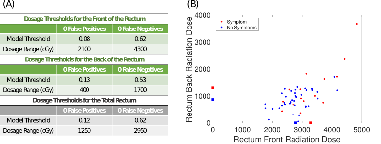
Figure 9: Logistic model thresholds and corresponding RT dosages for each rectum region. (A) Computed thresholds assuming independence. (B) Scatter plot for patients and their corresponding front and back RT doses. Patients with symptoms and without symptoms are shown in red and blue, respectively. The distribution of sampled RT doses are just broad enough to observe the that higher doses lead to symptoms. The mean front and back radiation doses of patients with and without symptoms are indicated by the thick red and blue bars on the $x$- and $y$-axes, respectively. The current data are insufficient to resolve anything other than a total dosage thresholding effect.

For the bladder, the dosage thresholds for the top and bottom of the bladder showed significant overlap: the top of the bladder could tolerate a dosage of 0-4,665 cGy while the bottom could tolerate a dosage of 3,183-5,387 cGy (see Appendix B). The corresponding scatter plot shows no discernible correlation between symptoms and sampled dosages.

4 Summary and Conclusions

With the lowering of the prostate cancer mortality rate, an emphasis has been placed on increasing the quality-of-life for patients undergoing radiation treatment. Utilizing machine learning algorithms and statistical methods, we provide an in-depth analysis on the spatial dosage provided to each patient. By analyzing a patient’s anatomical CT image and the radiation therapy dosing, we were able to connect understanding of how radiation influences secondary symptoms. We were able to do this by using a convolutional neural network that analyzed the CT image and associated radiation dosage. Our second method used ANOVA analysis on summarized spatial information. Using a brute-force technique, we were able to identify that splitting the bladder into a top region and bottom and the rectum into a front and back region was the best approach. Our outcomes from ANOVA agreed with our convolutional neural network and also provided dosage thresholds for each region. These results for the dosage thresholds for the rectum and bladder align with the results we obtained from our CNN prediction model, but should be interpreted with care. The thresholds across different regions should not be thought of as independent parameters because the dosages applied in the patient samples are correlated and the binary, whole patient symptom indicators are not attributed to any region. Moreover, the number of patients and the range of radiation doses they received are not large enough clearly resolve sharper thresholds. This explains the wide range for the bladder dosage thresholds and the overlap we observed between the top and bottom of the bladder. On the other hand, our CNN prediction model found that the radiation dosage (and the CT scan features) do in fact play a large role in explaining the differences in symptom development across patients.

In conclusion, we developed a deep learning framework and complementary statistical methods to identify the connection between spatial dosage and symptoms caused by prostate radiation therapy. A strength of machine learning is that it can produce accurate predictions if presented with sufficiently large data sets; however, the underlying mechanisms or specific features are difficult to discern in these approaches. In our application, it has the potential not only to accurately predict patient side effects, but also to learn what regions of the organs might be responsible for specific side effects. As is significant interest in integrating machine learning approaches with more traditional modeling approaches, we also found that classical statistical approaches was also useful in our problem. We expect that our CNN results will be much more accurate upon subsequent training on larger patient data sets and can be extended to predicting specific question scores to further refine treatment planning.

5 Acknowledgements

This research was funded by The Jayne Koskinas Ted Giovanis Foundation for Health and Policy and the Breast Cancer Research Foundation. TC acknowledges support from the Army Research Office through grant W911NF-18-1-0345 and the National Institutes of Health through grant R01HL146552 (TC). The authors also thank the Institute for Pure and Applied Mathematics at UCLA for hosting this project under the Research in Industrial Projects for Students program.

6 References

Appendix A Quality-of-Life Survey

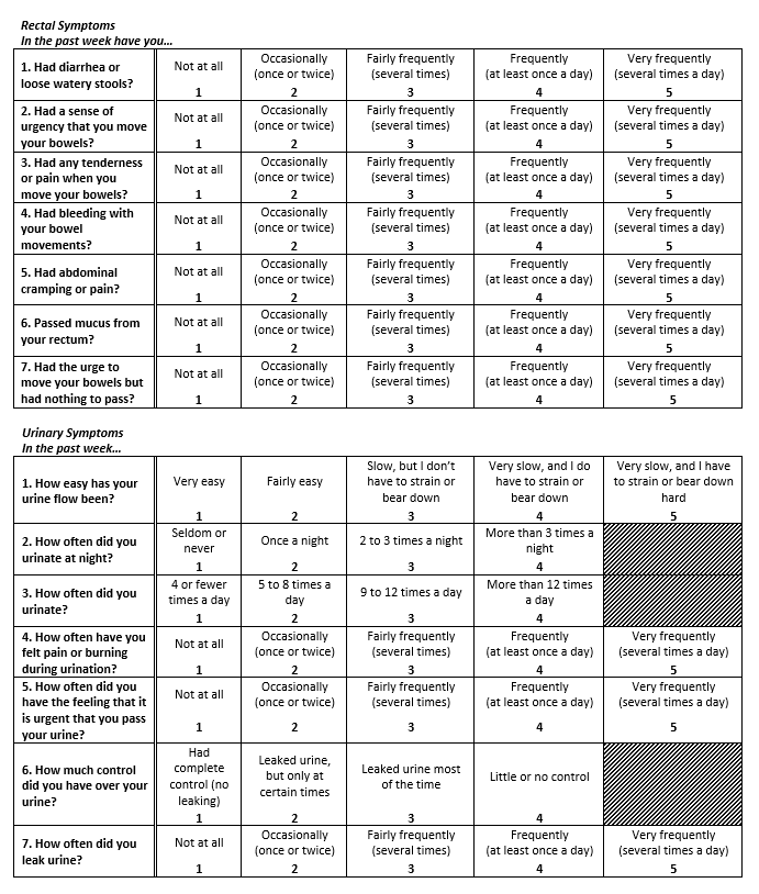
Figure 10: Quality-of-Life surveys given to patients before and weekly after RT.

Appendix B Bladder region thresholds

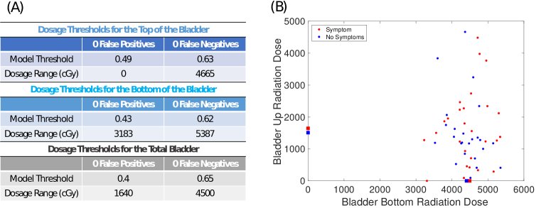
Figure 11: Logistic model thresholds and corresponding RT dosages for each bladder region. (A) Independently computed thresholds. These thresholds were estimated from logistic analysis with significant dosage overlap. that contained large overlap. (B) This is made clear in the scatter plot of RT doses to the top and bottom regions of bladder. For the bladder, there is a much smaller range in bottom bladder RT dose and no clear thresholds, i.e., the patients with and without symptoms have significant overlap in their RT dosages.

References

- [1] Massoud Al-Abany, Asgeir R. Helgason, Anna-Karin Agren Cronqvist, Bengt Lind, Panayiotis Mavroidis, Peter Wersäll, Helena Lind, Eva Qvanta, and Gunnar Steineck. Toward a definition of a threshold for harmless doses to the anal-sphincter region and the rectum. International Journal of Radiation OncologyBiologyPhysics, 61(4):1035–1044, 2005.
- [2] Anjali Balagopal, Samaneh Kazemifar, Dan Nguyen, Mu-Han Lin, Raquibul Hannan, Amir Owrangi, and Steve Jiang. Fully automated organ segmentation in male pelvic CT images. Physics in Medicine & Biology, 63(24):245015, 2018.
- [3] Ethan Basch. The missing voice of patients in drug-safety reporting. New England Journal of Medicine, 362(10):865–869, 2010. PMID: 20220181.
- [4] Kevin Diao, Emily A. Lobos, Eda Yirmibesoglu, Ram Basak, Laura H. Hendrix, Brittney Barbosa, Seth M. Miller, Kevin A. Pearlstein, Gregg H. Goldin, Andrew Z. Wang, and Ronald C. Chen. Patient-reported quality of life during definitive and postprostatectomy image-guided radiation therapy for prostate cancer. Practical Radiation Oncology, 7(2):e117–e124, 2017.
- [5] Bernd Fischer and Jan Modersitzki. A unified approach to fast image registration and a new curvature based registration technique. Linear Algebra and its Applications, 380:107–124, 2004.
- [6] Z. Jiang, J.-F. Witz, P. Lecomte-Grosbras, J. Dequidt, C. Duriez, M. Cosson, S. Cotin, and M. Brieu. B-spline Based Multi-organ Detection in Magnetic Resonance Imaging. Strain, 51(3):235–247, 2015.
- [7] Samaneh Kazemifar, Anjali Balagopal, Dan Nguyen, Sarah McGuire, Raquibul Hannan, Steve Jiang, and Amir Owrangi. Segmentation of the prostate and organs at risk in male pelvic CT images using deep learning. Biomedical Physics & Engineering Express, 4(5):055003, 2018.
- [8] Alex Krizhevsky, Ilya Sutskever, and Geoffrey E. Hinton. Imagenet classification with deep convolutional neural networks. Commun. ACM, 60(6):84–90, 2017.
- [9] Stuart Alexander MacGillivray. Curvature-based image registration: Review and extensions. mathesis, University of Waterloo, 2009.
- [10] Lawrence B. Marks, Ellen D. Yorke, Andrew Jackson, Randall K. Ten Haken, Louis S. Constine, Avraham Eisbruch, Søren M. Bentzen, Jiho Nam, and Joseph O. Deasy. Use of normal tissue complication probability models in the clinic. International Journal of Radiation Oncology *Biology *Physics, 76(3):S10–S19, 2010.
- [11] Panayiotis Mavroidis, Kevin A. Pearlstein, John Dooley, Jasmine Sun, Srinivas Saripalli, Shiva K. Das, Andrew Z. Wang, and Ronald C. Chen. Fitting ntcp models to bladder doses and acute urinary symptoms during post-prostatectomy radiotherapy. Radiation Oncology, 13(1):17, 2018.
- [12] Dan Nguyen, Troy Long, Xun Jia, Weiguo Lu, Xuejun Gu, Zohaib Iqbal, and Steve Jiang. Dose Prediction with U-net: A Feasibility Study for Predicting Dose Distributions from Contours using Deep Learning on Prostate IMRT Patients. arXiv, pages 1–18, 2018.
- [13] Dan Nguyen, Troy Long, Xun Jia, Weiguo Lu, Xuejun Gu, Zohaib Iqbal, and Steve Jiang. A feasibility study for predicting optimal radiation therapy dose distributions of prostate cancer patients from patient anatomy using deep learning. Scientific Reports, 9:1076, 2019.
- [14] Serguei V Pakhomov, Steven J Jacobsen, Christopher G Chute, and Veronique L Roger. Agreement between patient-reported symptoms and their documentation in the medical record. The American journal of managed care, 14(8):530–539, 2008.
- [15] Pranav Rajpurkar, Jeremy Irvin, Kaylie Zhu, Brandon Yang, Hershel Mehta, Tony Duan, Daisy Ding, Aarti Bagul, Curtis Langlotz, Katie Shpanskaya, Matthew P. Lungren, and Andrew Y. Ng. CheXNet: Radiologist-Level Pneumonia Detection on Chest X-Rays with Deep Learning. ArXiv, pages 1–7, 2017.
- [16] Olaf Ronneberger, Philipp Fischer, and Thomas Brox. U-net: Convolutional networks for biomedical image segmentation. In Nassir Navab, Joachim Hornegger, William M. Wells, and Alejandro F. Frangi, editors, Medical Image Computing and Computer-Assisted Intervention – MICCAI 2015, pages 234–241, Cham, 2015. Springer International Publishing.
- [17] Jeff A. Sloan, Lawrence Berk, Joseph Roscoe, Michael J. Fisch, Edward G. Shaw, Gwen Wyatt, Gary R. Morrow, and Amylou C. Dueck. Integrating patient-reported outcomes into cancer symptom management clinical trials supported by the national cancer institute–sponsored clinical trials networks. Journal of Clinical Oncology, 25(32):5070–5077, 2007. PMID: 17991923.
- [18] American Cancer Society. American cancer society facts & figures 2019, 2019. [Online; posted January 8 2019].
- [19] James A. Talcott, Jack A. Clark, Judith Manola, and Sonya P. Mitchell. Bringing prostate cancer quality of life research back to the bedside: Translating numbers into a format that patients can understand. Journal of Urology, 176(4):1558–1564, 2006.
- [20] Lynne I. Wagner, Lari Wenzel, Edward Shaw, and David Cella. Patient-Reported Outcomes in Phase II Cancer Clinical Trials: Lessons Learned and Future Directions. Journal of Clinical Oncology, 25(32):5058–5062, 2007. PMID: 17991921.