Divergence-Measure Fields:
Gauss-Green Formulas and Normal Traces

It is hard to imagine how most fields of science could provide the stunning mathematical descriptions of their theories and results if the integration by parts formula did not exist. Indeed, integration by parts is an indispensable fundamental operation, which has been used across scientific theories to pass from global (integral) to local (differential) formulations of physical laws. Even though the integration by parts formula is commonly known as the Gauss-Green formula (or the divergence theorem, or Ostrogradsky’s theorem), its discovery and rigorous mathematical proof are the result of the combined efforts of many great mathematicians, starting back the period when the calculus was invented by Newton and Leibniz in the 17th century.

The one-dimensional integration by parts formula for smooth functions was first discovered by Taylor (1715). The formula is a consequence of the Leibniz product rule and the Newton-Leibniz formula for the fundamental theorem of calculus.

The classical Gauss-Green formula for the multidimensional case is generally stated for $C^{1}$ vector fields and domains with $C^{1}$ boundaries. However, motivated by the physical solutions with discontinuity/singularity for Partial Differential Equations (PDEs) and Calculus of Variations, such as nonlinear hyperbolic conservation laws and Euler-Lagrange equations, the following fundamental issue arises:

Does the Gauss-Green formula still hold for vector fields with discontinuity/singularity $($such as divergence-measure fields$)$ and domains with rough boundaries?

The objective of this paper is to provide an answer to this issue and to present a short historical review of the contributions by many mathematicians spanning more than two centuries, which have made the discovery of the Gauss-Green formula possible.

The Classical Gauss-Green Formula

The Gauss-Green formula was originally motivated in the analysis of fluids, electric and magnetic fields, and other problems in the sciences in order to establish the equivalence of integral and differential formulations of various physical laws. In particular, the derivations of the Euler equations and the Navier-Stokes equations in Fluid Dynamics and Gauss’s laws for the electronic and magnetic fields are based on the validity of the Gauss-Green formula and associated Stokes theorem. As an example, see Fig. 1 for the derivation of the Euler equation for the conservation of mass in the smooth case.

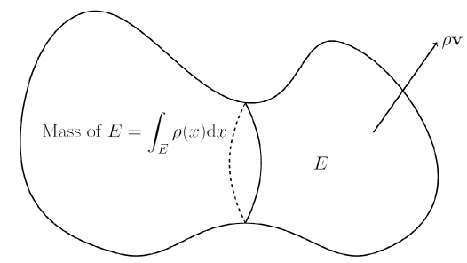
Figure 1. Conservation of mass: The rate of change of the total mass in an open set $E$, $\frac{{\rm d}}{{\rm d}t}\int_{E}\rho(t,x)\,{\rm d}x$, is equal to the total flux of mass across boundary $\partial E$, $\int_{\partial E}(\rho\mathbf{v})\cdot\nu\,{\rm d}{\mathscr{H}}^{n-1}$, where $\rho$ is the density, $\mathbf{v}$ is the velocity field, and the boundary value of $(\rho\mathbf{v})\cdot\nu$ is regarded as the normal trace of the vector field $\rho\mathbf{v}$ on $\partial E$. The Gauss-Green formula yields the Euler equation for the conservation of mass: $\rho_{t}+\text{\sl div}(\rho\mathbf{v})=0$ in the smooth case.

The formula that is also later known as the divergence theorem was first discovered by Lagrange in 1762 (see Fig. 3), however, he did not provide a proof of the result. The theorem was later rediscovered by Gauss in 1813 (see Fig. 3) and Ostrogradsky in 1828 (see Fig. 4). Ortrogradsky’s method of proof was similar to the approach Gauss used. Independently, Green (see Fig. 5) also rediscovered the divergence theorem in the two-dimensional case and published his result in 1828.

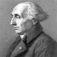
Figure 2. Joseph-Louis Lagrange (25 January 1736 – 10 April 1813)

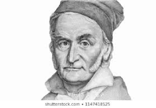
Figure 3. Carl Friedrich Gauss (30 April 1777 – 23 February 1855)

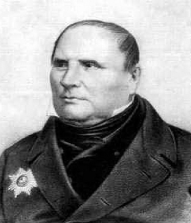
Figure 4. Mikhail Ostrogradsky (24 September 1801 – 1 January 1862)

Figure 5. The title page of the original essay of George Green (14 July 1793 – 31 May 1841)

The divergence theorem in its vector form for the $n$–dimensional case $(n\geq 2)$ can be stated as

$$\int_{E}\text{\sl div}{\bm{F}}\,{\rm d}y=-\int_{\partial E}{\bm{F}}\cdot\nu\,{\rm d}{\mathscr{H}}^{n-1},$$ (1)

where ${\bm{F}}$ is a $C^{1}$ vector field, $E$ is a bounded open set with piecewise smooth boundary, $\nu$ is the inner unit normal vector to $E$, the boundary value of ${\bm{F}}\cdot\nu$ is regarded as the normal trace of the vector field ${\bm{F}}$ on $\partial E$, and ${\mathscr{H}}^{n-1}$ is the $(n-1)$–dimensional Hausdorff measure (that is an extension of the surface area measure for $2$–dimensional surfaces to general $(n-1)$–dimensional boundaries $\partial E$). The formulation of (1), where ${\bm{F}}$ represents a physical vector quantity, is also the result of the efforts of many mathematicians including Gibbs, Heaviside, Poisson, Sarrus, Stokes, and Volterra. In conclusion, formula (1) is the result of more than two centuries of efforts by great mathematicians!

Gauss-Green Formulas and Traces for Lipschitz Vector Fields
on Sets of Finite Perimeter

We first go back to the issue arisen earlier for extending the Gauss-Green formula to very rough sets. The development of Geometric Measure Theory in the middle of the 20th century opened the door to the extension of the classical Gauss-Green formula over sets of finite perimeter (whose boundaries can be very rough and contain cusps, corners, among others; cf. Fig. 6) for Lipschitz vector fields.

Indeed, we may consider the left side of (1) as a linear functional acting on vector fields ${\bm{F}}\in C_{c}^{1}(\mathbb{R}^{n})$. If $E$ is such that the functional: ${\bm{F}}\to\int_{E}\text{\sl div}{\bm{F}}\,{\rm d}y$ is bounded on $C_{c}(\mathbb{R}^{n})$, then the Riesz representation theorem implies that there exists a Radon measure $\mu_{E}$ such that

$$\int_{E}\text{\sl div}{\bm{F}}\,{\rm d}y=\int_{\mathbb{R}^{n}}{\bm{F}}\cdot{\rm d}\mu_{E}\qquad\,\,\text{ for all }{\bm{F}}\in C_{c}^{1}(\mathbb{R}^{n}),$$ (2)

and the set, $E$, is called a set of finite perimeter in $\mathbb{R}^{n}$. In this case, the Radon measure $\mu_{E}$ is actually the gradient of $-\chi_{E}$ (strictly speaking, the gradient is in the distributional sense), where $\chi_{E}$ is the characteristic function of $E$. A set of density $\alpha\in[0,1]$ of $E$ in $\mathbb{R}^{n}$ is defined by

$$E^{\alpha}:=\big{\{}y\in\mathbb{R}^{n}:\lim_{r\to 0}\frac{|B_{r}(y)\cap E|}{|B_{r}(y)|}=\alpha\big{\}},$$ (3)

where $|B|$ represents the Lebesgue measure of any Lebesgue measurable set $B$. Then $E^{0}$ is the measure-theoretic exterior of $E$, while $E^{1}$ is the measure-theoretic interior of $E$.

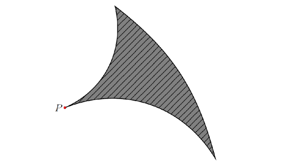
Figure 6. $E$ is an open set of finite perimeter where cusp $P$ is a point of density $0$

Sets of finite perimeter can be quite subtle. For example, the countable union of open balls with centers on the rational points $y_{k}$, $k=1,2,\dots$, of the unit ball in $\mathbb{R}^{n}$ and with radius $2^{-k}$, is a set of finite perimeter. A set of finite perimeter may have a large set of cusps in the topological boundary (e.g., ${\mathscr{H}}^{n-1}(E^{0}\cap\partial E)>0$ or ${\mathscr{H}}^{n-1}(E^{1}\cap\partial E)>0$). The set $E$ can also have points in the boundary which belong $E^{\alpha}$ for $\alpha\notin\{0,1\}$. For example, the four corners of a square are points of density $\frac{1}{4}$.

Even though the boundary of a set $E$ of finite perimeter can be very rough, De Giorgi’s structure theorem indicates that it has nice tangential properties so that there is a notion of measure-theoretic tangent plane. More rigorously, the topological boundary $\partial E$ of $E$ contains an $(n-1)$–rectifiable set, known as the reduced boundary of $E$, denoted as $\partial^{*}E$, which can be covered by a countable union of $C^{1}$ surfaces, up to a set of ${\mathscr{H}}^{n-1}$–measure zero. More generally, Federer’s theorem states that ${\mathscr{H}}^{n-1}(\partial^{s}E\setminus\partial^{*}E)=0$, where $\partial^{s}E=\mathbb{R}^{n}\setminus(E^{0}\cup E^{1})$ is called the essential boundary. Note that $\partial^{*}E\subset E^{\frac{1}{2}}$ and $\partial^{*}E\subset\partial^{s}E\subset\partial E$.

It can be shown that every $y\in\partial^{*}E$ has an inner unit normal vector $\nu_{E}(y)$ and a tangent plane in the measure-theoretic sense, and (2) reduces to

$$\int_{E}\text{\sl div}{\bm{F}}\,{\rm d}y=-\int_{\partial^{*}E}{\bm{F}}(y)\cdot\nu_{E}(y)\,{\rm d}\mathscr{H}^{n-1}(y).$$ (4)

This Gauss-Green formula for Lipschitz vector fields ${\bm{F}}$ over sets of finite perimeter was proved by De Giorgi (1954–55) and Federer (1945, 1958) in a series of papers. See [13, 15] and the references therein.

Gauss-Green Formulas and Traces for Sobolev and $BV$ Functions
on Lipschitz Domains

It happens in many areas of analysis, such as PDEs and Calculus of Variations, that it is necessary to work with the functions that are not Lipschitz, but only in $L^{p}$, $1\leq p\leq\infty$. In many of these cases, the functions have weak derivatives that also belong to $L^{p}$. That is, the corresponding ${\bm{F}}$ in (4) is a Sobolev vector field. The necessary and sufficient conditions for the existence of traces (i.e., boundary values) of Sobolev functions defined on the boundary of the domain have been obtained so that (4) is a valid formula over open sets with Lipschitz boundary.

The development of the theory of Sobolev spaces has been fundamental in analysis. However, for many further applications, this theory is still not sufficient. For example, the characteristic function of a set $E$ of finite perimeter, $\chi_{E}$, is not a Sobolev function. Physical solutions in gas dynamics involve shock waves and vortex sheets that are discontinuities with jumps. Thus, a larger space of functions, called the space of functions of bounded variation ($BV$), is necessary, which consists of all functions in $L^{1}$ whose derivatives are Radon measures.

This space has compactness properties that allow, for instance, to show the existence of minimal surfaces and the well-posedness of $BV$ solutions for hyperbolic conservation laws. Moreover, the Gauss-Green formula (4) is also valid for $BV$ vector fields over Lipschitz domains. See [13, 14, 20] and the references therein.

Divergence-Measure Fields and Hyperbolic Conservation Laws

A vector field ${\bm{F}}\in L^{p}(\Omega)$, $1\leq p\leq\infty$, is called a divergence-measure field if $\text{\sl div}{\bm{F}}$ is a signed Radon measure with finite total variation in $\Omega$. Such vector fields form Banach spaces, denoted as $\mathcal{DM}^{p}(\Omega)$, for $1\leq p\leq\infty$.

These spaces arise naturally in the field of Hyperbolic Conservation Laws. Consider hyperbolic systems of conservation laws of the form:

$${\bf u}_{t}+\nabla_{x}\cdot{\bf f}({\bf u})=0\qquad\,\,\,\,\mbox{for ${\bf u}=(u_{1},...,u_{m})^{\top}:\mathbb{R}^{n}\to\mathbb{R}^{m}$}$$ (5)

where $(t,x)\in\mathbb{R}_{+}^{n}:=[0,\infty)\times\mathbb{R}^{d}$, $n:=d+1,{\bf f}=({\bf f}_{1},{\bf f}_{2},...,{\bf f}_{d})$, and ${\bf f}_{j}:\mathbb{R}^{m}\to\mathbb{R}^{m},j=1,\cdots,d$. A prototype of such systems is the system of Euler equations for compressible fluids, which consists of the conservation equations of mass, momentum, and energy in Continuum Mechanics such as Gas Dynamics and Elasticity. One of the main features of the hyperbolic system is that the speeds of propagation of solutions are finite; another feature is that, no matter how smooth a solution starts with initially, it generically develops singularity and becomes a discontinuous/singular solution. To single out physically relevant solutions, it requires the solutions of system (5) to fall within the following class of entropy solutions:

An entropy solution ${\bf u}(t,x)$ of system (5) is characterized by the Lax entropy inequality: For any entropy pair $(\eta,{\bf q})$ with $\eta$ being a convex function of ${\bf u}$,

$$\eta({\bf u}(t,x))_{t}+\nabla_{x}\cdot{\bf q}({\bf u}(t,x))\leq 0\qquad\textnormal{\it in the sense of distributions}.$$ (6)

Here, a function $\eta\in C^{1}(\mathbb{R}^{m},\mathbb{R})$ is called an entropy of system (5) if there exists an entropy flux ${\bf q}=(q_{1},\cdots,q_{d})\in C^{1}(\mathbb{R}^{m},\mathbb{R}^{d})$ such that

$$\nabla q_{j}({\bf u})=\nabla\eta({\bf u})\nabla{\bf f}_{j}({\bf u})\qquad\,\,\mbox{for $j=1,2,...,d$}.$$ (7)

Then $(\eta,{\bf q})({\bf u})$ is called an entropy pair of system (5).

Friedrichs-Lax (1971) observed that most systems of conservation laws that result from Continuum Mechanics are endowed with a globally defined, strictly convex entropy. In particular, for the compressible Euler equations in Lagrangian coordinates, $\eta=-S$ is such an entropy, where $S$ is the physical thermodynamic entropy of the fluid. Then the Lax entropy inequality for the physical entropy $\eta=-S$ is an exact statement of the Second Law of Thermodynamics (cf. [3, 11]). Similar notions of entropy have also been used in many fields such as Kinetic Theory, Statistical Physics, Ergodic Theory, Information Theory, and Stochastic Analysis.

Indeed, the available existence theories show that the solutions of (5) are entropy solutions obeying the Lax entropy inequality (6). This implies that, for any entropy pair $(\eta,{\bf q})$ with $\eta$ being a convex function, there exists a nonnegative measure $\mu_{\eta}\in\mathcal{M}(\mathbb{R}_{+}^{n})$ such that

$$\text{\sl div}_{(t,x)}(\eta({\bf u}(t,x)),{\bf q}({\bf u}(t,x)))=-\mu_{\eta}.$$ (8)

Moreover, for any $L^{\infty}$ entropy solution ${\bf u}$, if the system is endowed with a strictly convex entropy, then, for any $C^{2}$ entropy pair $(\eta,{\bf q})$ (not necessarily convex for $\eta$), there exists a signed Radon measure $\mu_{\eta}\in\mathcal{M}(\mathbb{R}_{+}^{n})$ such that (8) still holds (see [3]). For these cases, $(\eta({\bf u}),{\bf q}({\bf u}))(t,x)$ is a $\mathcal{DM}^{p}(\mathbb{R}_{+}^{n})$ vector field, as long as $(\eta({\bf u}),{\bf q}({\bf u}))(t,x)\in L^{p}(\mathbb{R}_{+}^{n},\mathbb{R}^{n})$ for some $p\in[1,\infty]$.

Equation (8) is one of the main motivations to develop a $\mathcal{D}\mathcal{M}$ theory in Chen-Frid [5, 6]. In particular, one of the major issues is whether integration by parts can be performed in (6) to explore to fullest extent possible all the information about the entropy solution ${\bf u}$. Thus, a concept of normal traces for $\mathcal{D}\mathcal{M}$ fields ${\bm{F}}$ is necessary to be developed. The existence of normal traces is also fundamental for initial-boundary value problems for hyperbolic systems (5) and for the analysis of structure and regularity of entropy solutions ${\bf u}$ (see e.g. [3, 5, 6, 11, 19]).

Motivated by hyperbolic conservation laws, the interior and exterior normal traces need to be constructed as the limit of classical normal traces on one-sided smooth approximations of the domain. Then the surface of a shock wave or vortex sheet can be approximated with smooth surfaces to obtain the interior and exterior fluxes on the shock wave or vortex sheet.

Other important connections for the $\mathcal{D}\mathcal{M}$ theory are the characterization of phase transitions (coexistent phases with discontinuities across the boundaries), the concept of stress, the notion of Cauchy flux, and the principle of balance law to accommodate the discontinuities and singularities in the continuum media in Continuum Mechanics, as discussed in Degiovanni-Marzocchi-Musesti [12], Šilhavý [16, 17], Chen-Torres-Ziemer [9], and Chen-Comi-Torres [4].

Gauss-Green Formulas and Normal Traces for $\mathcal{DM}^{\infty}$ Fields

We start with the following simple example:

Example 1. Consider the vector field ${\bm{F}}:\Omega=\mathbb{R}^{2}\cap\{y_{1}>0\}\to\mathbb{R}^{2}$:

$${\bm{F}}(y_{1},y_{2})=(0,\sin(\frac{1}{y_{1}})).$$ (9)

Then ${\bm{F}}\in\mathcal{D}\mathcal{M}^{\infty}(\Omega)$ with $\text{\sl div}{\bm{F}}=0$ in $\Omega$.

However, in an open half-disk $E=\{(y_{1},y_{2})\,:\,y_{1}>0,y_{1}^{2}+y_{2}^{2}<1\}\subset\Omega$, the previous Gauss-Green formulas do not apply. Indeed, since ${\bm{F}}(y_{1},y_{2})$ is highly oscillatory when $y_{1}\to 0$ which is not well-defined at $y_{1}=0$, it is not clear how the normal trace ${\bm{F}}\cdot\nu$ on $\{y_{1}=0\}$ can be understood in the classical sense so that the equality between $\int_{E}\text{\sl div}{\bm{F}}\,{\rm d}{\mathscr{H}}^{n-1}=0$ and $\int_{\partial E}{\bm{F}}\cdot\nu\,{\rm d}{\mathscr{H}}^{n-1}$ holds. This example shows that a suitable notion of normal traces is required to be developed.

A generalization of (1) to $\mathcal{D}\mathcal{M}^{\infty}(\Omega)$ fields and bounded sets with Lipschitz boundary was derived in Anzellotti [1] and Chen-Frid [5] by different approaches. A further generalization of (1) to $\mathcal{D}\mathcal{M}^{\infty}(\Omega)$ fields and arbitrary bounded sets of finite perimeter, $E\Subset\Omega$, was first obtained in Chen-Torres [8] and Šilhavý [16] independently; see also [9, 10].

Theorem 1. Let $E$ be a set of finite perimeter. Then

$$\int_{E^{1}}\phi\,{\rm d\hskip 0.28453pt}\text{\sl div}{\bm{F}}+\int_{E^{1}}{\bm{F}}\cdot\nabla\phi\,{\rm d}y=-\int_{\partial^{*}E}\phi\,\mathfrak{F}_{\rm i}\cdot\nu_{E}\,{\rm d}{\mathscr{H}}^{n-1}\qquad\mbox{for every $\phi\in C_{c}^{1}(\mathbb{R}^{n})$},$$ (10)

where the interior normal trace $\mathfrak{F}_{\rm i}\cdot\nu_{E}$ is a bounded function defined on the reduced boundary of $E$ (i.e., $\mathfrak{F}_{\rm i}\cdot\nu_{E}\in L^{\infty}(\partial^{*}E;{\mathscr{H}}^{n-1})$), and $E^{1}$ is the measure-theoretic interior of $E$ as defined in (3).

One approach for the proof of (10) is based on a product rule for $\mathcal{D}\mathcal{M}^{\infty}$ fields (see [8]). Another approach in [9], following [5], is based on a new approximation theorem for sets of finite perimeter, which shows that the level sets of convolutions $w_{k}:=\chi_{E}*\varrho_{k}$ by the standard positive and symmetric mollifiers provide smooth approximations essentially from the interior (by choosing $w_{k}^{-1}(t)$ for $\frac{1}{2}<t<1$) and the exterior (for $0<t<\frac{1}{2}$). Thus, the interior normal trace $\mathfrak{F}_{\rm i}\cdot\nu_{E}$ is constructed as the limit of classical normal traces over the smooth approximations of $E$. Since the level set $w_{k}^{-1}(t)$ (with a suitable fixed $0<t<\frac{1}{2}$) can intersect the measure-theoretic exterior $E^{0}$ of $E$, a critical step for this approach is to show that ${\mathscr{H}}^{n-1}(w_{k}^{-1}(t)\cap E^{0})$ converges to zero as $k\to\infty$. A key point for this proof is the fact that, if ${\bm{F}}$ is a $\mathcal{D}\mathcal{M}^{\infty}$ field, then the Radon measure $|\text{\sl div}{\bm{F}}|$ is absolutely continuous with respect to ${\mathscr{H}}^{n-1}$, as first observed by Chen-Frid [5].

If $E=\{y\in\mathbb{R}^{2}\,:\,|y|<1\}\setminus\{y_{1}>0,y_{2}=0\}$, the above formulas apply, but the integration is not over the original representative consisting of the disk with radius $\{y_{1}>0,y_{2}=0\}$ removed, since $E^{1}=\{y\in\mathbb{R}^{2}\,:\,|y|<1\}$ is the open disk. In many applications including those in Materials Science, we may want to integrate on a domain with fractures or cracks; see also Fig. 7. Since the cracks are part of the topological boundary and belong to the measure-theoretic interior $E^{1}$, the formulas in (10) do not provide such information. In order to establish a Gauss-Green formula that includes such cases, we restrict to open sets $E$ of finite perimeter with ${\mathscr{H}}^{n-1}(\partial E\setminus E^{0})<\infty$. Therefore, $\partial E$ can still have a large set of cusps or points of density $0$ (i.e., points belonging to $E^{0}$).

Figure 7. $E$ is an open set with several fractures (dotted lines)

It has been shown in [7] that, if $E$ is a bounded open set satisfying

$${\mathscr{H}}^{n-1}(\partial E\setminus E^{0})<\infty,$$ (11)

and ${\bm{F}}\in\mathcal{DM}^{\infty}(E)$, then there exists a family of sets $E_{k}\Subset E$ such that $E_{k}\to E$ in $L^{1}$ and $\sup_{k}{\mathscr{H}}^{n-1}(\partial^{*}E_{k})<\infty$ such that, for any $\phi\in C_{c}^{1}(\mathbb{R}^{n})$,

$$\int_{E}\phi\,{\rm d\hskip 0.28453pt}\text{\sl div}{\bm{F}}+\int_{E}{\bm{F}}\cdot\nabla\phi\,{\rm d}y=-\lim_{k\to\infty}\int_{\partial E_{k}}\phi{\bm{F}}\cdot\nu_{E_{k}}\,\,{\rm d}{\mathscr{H}}^{n-1}=\int_{\partial E\setminus E^{0}}\phi\,\mathfrak{F}\cdot\nu_{E}\,{\rm d}{\mathscr{H}}^{n-1},$$ (12)

where $\mathfrak{F}\cdot\nu_{E}$ is well-defined in $L^{\infty}(\partial E\setminus E^{0};{\mathscr{H}}^{n-1})$ as the interior normal trace on $\partial E\setminus E^{0}$.

This approximation result for the bounded open set $E$ can be accomplished by performing delicate covering arguments, especially by applying the Besicovitch theorem to a covering of $\partial E\cap E^{0}$. Moreover, (12) is a formula up to the boundary, since we do not assume that the domain of integration is compactly contained in the domain of ${\bm{F}}$. More general product rules for $\text{\sl div}(\phi{\bm{F}})$ can be proved to weaken the regularity of $\phi$; see [4, 7] and the references therein.

Gauss-Green Formulas and Normal Traces for $\mathcal{DM}^{p}$ Fields

For $\mathcal{D}\mathcal{M}^{p}$ fields with $1\leq p<\infty$, the situation becomes more delicate.

Example 2 (Whitney [Example 1, p. 100]). Consider the vector field ${\bm{F}}:\mathbb{R}^{2}\setminus\{(0,0)\}\to\mathbb{R}^{2}$ $($see Fig. 9$)$:

$${\bm{F}}(y_{1},y_{2})=\frac{(y_{1},y_{2})}{y_{1}^{2}+y_{2}^{2}}.$$ (13)

Then ${\bm{F}}\in\mathcal{D}\mathcal{M}^{p}_{\rm loc}(\mathbb{R}^{2})$ for $1\leq p<2$. If $E=(0,1)^{2}$, it is observed that

$$0=\text{\sl div}{\bm{F}}(E)\neq-\int_{\partial E}{\bm{F}}\cdot\nu_{E}\,{\rm d}{\mathscr{H}}^{1}=\frac{\pi}{2},$$

where $\nu_{E}$ is the inner unit normal to the square. However, if $E_{\varepsilon}:=\{y\in E\,:\,{\rm dist}(y,\partial E)>\varepsilon\}$ and $E^{\varepsilon}:=\{y\in\mathbb{R}^{n}\,:\,{\rm dist}(y,E)<\varepsilon\}$ for any $\varepsilon>0$, then

$$0=\text{\sl div}{\bm{F}}(E)=-\lim_{\varepsilon\to 0}\int_{\partial E_{\varepsilon}}{\bm{F}}\cdot\nu_{E_{\varepsilon}}\,{\rm d}{\mathscr{H}}^{1},$$

$$2\pi=\text{\sl div}{\bm{F}}(\overline{E})=-\lim_{\varepsilon\to 0}\int_{\partial E^{\varepsilon}}{\bm{F}}\cdot\nu_{E^{\varepsilon}}\,{\rm d}{\mathscr{H}}^{1}.$$

In this sense, the equality is achieved on both sides of the formula.

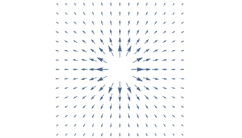
Figure 8. The vector field ${\bm{F}}(y_{1},y_{2})=\frac{(y_{1},y_{2})}{y_{1}^{2}+y_{2}^{2}}$ in Example 2

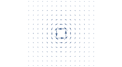
Figure 9. The vector field ${\bm{F}}(y_{1},y_{2})=\frac{(-y_{2},y_{1})}{y_{1}^{2}+y_{2}^{2}}$ in Example 3

Indeed, for a $\mathcal{D}\mathcal{M}^{p}$ field with $p\neq\infty$, $|\text{\sl div}{\bm{F}}|$ is absolutely continuous with respect to ${\mathscr{H}}^{n-p^{\prime}}$ for $p^{\prime}>1$ with $\frac{1}{p^{\prime}}+\frac{1}{p}=1$, but not with respect to ${\mathscr{H}}^{n-1}$ in general. This implies that the approach in [9] does not apply directly to obtain normal traces for $\mathcal{DM}^{p}$ fields for $p\neq\infty$.

Then the following questions arise:

• Can the previous formulas be proved in general for any ${\bm{F}}\in\mathcal{DM}^{p}(\Omega)$ and for any open set $E\subset\Omega$?

• Even though almost all the level sets of the distance function are sets of finite perimeter, can the formulas with smooth approximations of $E$ be obtained, in place of $E_{\varepsilon}$ and $E^{\varepsilon}$?

• If $E$ has a Lipschitz boundary, do regular Lipschitz deformations of $E$, as defined in Chen-Frid [5, 6], exist?

The answer to all three questions is affirmative.

Theorem 2 (Chen-Comi-Torres [4]). Let $E\subset\Omega$ be a bounded open set, and let ${\bm{F}}\in\mathcal{D}\mathcal{M}^{p}(\Omega)$ for $1\leq p\leq\infty$. Then, for any $\phi\in(C^{0}\cap L^{\infty})(\Omega)$ with $\nabla\phi\in L^{p^{\prime}}(\Omega;\mathbb{R}^{n})$ for $p^{\prime}\geq 1$ so that $\frac{1}{p^{\prime}}+\frac{1}{p}=1$, there exists a sequence of bounded open sets $E_{k}$ with $C^{\infty}$ boundary such that $E_{k}\Subset E$, $\bigcup_{k}E_{k}=E$, and

$$\int_{E}\phi\,{\rm d\hskip 0.28453pt}\text{\sl div}{\bm{F}}+\int_{E}{\bm{F}}\cdot\nabla\phi\,{\rm d}y=-\lim_{k\to\infty}\int_{\partial E_{k}}\phi{\bm{F}}\cdot\nu_{E_{k}}\,\,{\rm d}{\mathscr{H}}^{n-1},$$ (14)

where $\nu_{E_{k}}$ is the classical inner unit normal vector to $E_{k}$.

For the open set $E$ with Lipschitz boundary, it can be proved that the deformations of $E$ obtained with the method of regularized distance are bi-Lipschitz. We can also employ an alternative construction by Nečas (1962) to obtain smooth approximations $E_{\varepsilon}$ of a bounded open set $E$ with Lipschitz boundary in such a way that the deformation, $\Psi_{\varepsilon}(x)$, mapping $\partial E$ to $\partial E_{\varepsilon}$ is bi-Lipschitz, and the Jacobians of the deformations, $J^{\partial E}(\Psi_{\varepsilon})$, converge to $1$ in $L^{1}(\partial E)$ as $\varepsilon$ approaches zero (see [4, Theorem 8.19]). This shows that any bounded open set with Lipschitz boundary admits a regular Lipschitz deformation in the sense of Chen-Frid [5, 6]. Therefore, we can write more explicit Gauss-Green formulas for Lipschitz domains.

Theorem 3 (Chen-Comi-Torres [4]). If $E\Subset\Omega$ is an open set with Lipschitz boundary and ${\bm{F}}\in\mathcal{D}\mathcal{M}^{p}(\Omega)$ for $1\leq p\leq\infty$, then, for every $\phi\in C^{0}(\Omega)$ with $\nabla\phi\in L^{p^{\prime}}(\Omega;\mathbb{R}^{n})$, there exists a set $\mathcal{N}\subset\mathbb{R}$ of Lebesgue measure zero such that, for every nonnegative sequence $\{\varepsilon_{k}\}\not\subset\mathcal{N}$ satisfying $\varepsilon_{k}\to 0$,

$$\int_{E}\phi\,{\rm d\hskip 0.28453pt}\text{\sl div}{\bm{F}}+\int_{E}{\bm{F}}\cdot\nabla\phi\,{\rm d}y=-\lim_{k\to\infty}\int_{\partial E}\big{(}\phi{\bm{F}}\cdot\frac{\nabla\rho}{|\nabla\rho|}\big{)}(\Psi_{\varepsilon_{k}}(y))J^{\partial E}(\Psi_{\varepsilon_{k}})(y)\,{\rm d}{\mathscr{H}}^{n-1}(y),$$

where $\rho(y)\in C^{2}(\mathbb{R}^{n}\setminus\partial E)\cap{\rm Lip(\mathbb{R}^{n})}$ is a regularized distance for $E$, so that the ratio functions $\frac{\rho(y)}{d(y)}$ and $\frac{d(y)}{\rho(y)}$ are positive and uniformly bounded for all $y\in\mathbb{R}^{n}\setminus\partial U$ for $d(y)$ to be ${\rm dist}(y,\partial E)$ for $y\in E$ and $-{\rm dist}(y,\partial E)$ for $y\notin E$.

The question now arises as to whether the limit can be realized on the right hand side of the previous formulas as an integral on $\partial E$. In general, this is not possible. However, in some cases, it is possible to represent the normal trace with a measure supported on $\partial E$. In order to see this, for ${\bm{F}}\in\mathcal{D}\mathcal{M}^{p}(\Omega)$, $1\leq p\leq\infty$, and a bounded Borel set $E\subset\Omega$, we follow [1, 6, 16] to define the normal trace distribution of ${\bm{F}}$ on $\partial E$ as

$$\left\langle{\bm{F}}\cdot\nu,\phi\right\rangle_{\partial E}:=\int_{E}\phi\,{\rm d}\text{\sl div}{\bm{F}}+\int_{E}{\bm{F}}\cdot\nabla\phi\,{\rm d}y\qquad\mbox{for any $\phi\in\text{\rm Lip}_{c}(\mathbb{R}^{n})$}.$$ (15)

The formula presented above shows that the trace distribution on $\partial E$ can be extended to a functional on $\{\phi\in(C^{0}\cap L^{\infty})(\Omega):\nabla\phi\in L^{p^{\prime}}(\Omega,\mathbb{R}^{n})\}$ so that we can always represent the normal trace distribution as the limit of classical normal traces on smooth approximations of $E$. Then the question is whether there exists a Radon measure $\mu$ concentrated on $\partial E$ such that $\left\langle{\bm{F}}\cdot\nu,\phi\right\rangle_{\partial E}=\int_{\partial E}\phi\,{\rm d}\mu$. Unfortunately, this not the case in general.

Example 3. Consider the vector field ${\bm{F}}:\mathbb{R}^{2}\setminus\{(0,0)\}\to\mathbb{R}^{2}$:

$${\bm{F}}(y_{1},y_{2})=\frac{(-y_{2},y_{1})}{(y_{1}^{2}+y_{2}^{2})^{\alpha/2}}\qquad\mbox{for $1\leq\alpha<3$}.$$

Then ${\bm{F}}\in\mathcal{DM}_{\rm loc}^{p}(\mathbb{R}^{2})$ with $1\leq p<\frac{2}{\alpha-1}$ for $1<\alpha<3$, and $p=\infty$ for $\alpha=1$, and $\text{\sl div}{\bm{F}}=0$ on $E=(-1,1)\times(-1,0)$. For $\phi\in{\rm Lip}(\partial E)$ with ${\rm supp}\,\phi\subset\{y_{2}=0,|y_{1}|<1\}$, as shown in Šilhavý [18, Example 2.5],

$$\left\langle{\bm{F}}\cdot\nu,\phi\right\rangle_{\partial E}:=\begin{cases}\int_{-1}^{1}\phi(t,0){\rm sgn}(t)|t|^{1-\alpha}{\rm d\hskip 0.28453pt}t\qquad&\mbox{for $1\leq\alpha<2$},\\[4.2679pt] \lim_{\varepsilon\to 0}\int_{\{|t|>\varepsilon\}}\phi(t,0){\rm sgn}(t)|t|^{1-\alpha}{\rm d\hskip 0.28453pt}t\qquad&\mbox{for $2\leq\alpha<3$}.\end{cases}$$

This indicates that the normal trace $\left\langle{\bm{F}}\cdot\nu,\cdot\right\rangle_{\partial E}$ of the vector field ${\bm{F}}(y_{1},y_{2})$ is a measure when $1\leq\alpha<2$, but is not a measure when $2\leq\alpha<3$. Also see Fig. 9 when $\alpha=2$.

Indeed, it can be shown (see [4, Theorem 4.1]) that $\left\langle{\bm{F}}\cdot\nu,\phi\right\rangle_{\partial E}$ can be represented as a measure if and only if $\chi_{E}{\bm{F}}\in\mathcal{D}\mathcal{M}^{p}(\Omega)$. Moreover, if $\left\langle{\bm{F}}\cdot\nu,\cdot\right\rangle_{\partial E}$ is a measure, then

• For $p=\infty$, $|\left\langle{\bm{F}}\cdot\nu,\cdot\right\rangle_{\partial E}|\ll{\mathscr{H}}^{n-1}\mathop{\hbox{\vrule height=7.0pt,width=0.5pt,depth=0.0pt\vrule height=0.5pt,width=6.0pt,depth=0.0pt}}\nolimits\partial E$ (i.e., ${\mathscr{H}}^{n-1}$ restricted to $\partial E$) (see [5, Proposition 3.1]);

• For $\frac{n}{n-1}\leq p<\infty$, $|\left\langle{\bm{F}}\cdot\nu,\cdot\right\rangle_{\partial E}|(B)=0$ for any Borel set $B\subset\partial E$ with $\sigma$–finite ${\mathscr{H}}^{n-p^{\prime}}$ measure (see [16, Theorem 3.2(i)]).

This characterization can be used to find classes of vector fields for which the normal trace can be represented by a measure. An important observation is that, for a constant vector field ${\bm{F}}\equiv{\bm{v}}\in\mathbb{R}^{n}$,

$$\left\langle{\bm{v}}\cdot\nu,\cdot\right\rangle_{\partial E}=-\text{\sl div}(\chi_{E}{\bm{v}})=-\sum_{j=1}^{n}v_{j}D_{y_{j}}\chi_{E}.$$

Thus, in order that $\sum_{j=1}^{n}v_{j}D_{y_{j}}\chi_{E}$ is a measure, it is not necessary to assume that $\chi_{E}$ is a $BV$ function, since cancellations could be possible so that the previous sum could still be a measure. Indeed, such an example has been constructed (see [4, Remark 4.14]) for a set $E\subset\mathbb{R}^{2}$ without finite perimeter and a vector field ${\bm{F}}\in\mathcal{DM}^{p}(\mathbb{R}^{2})$ for any $p\in[1,\infty]$ such that the normal trace of ${\bm{F}}$ is a measure on $\partial E$.

In general, even for an open set with smooth boundary, $\left\langle{\bm{F}}\cdot\nu,\cdot\right\rangle_{\partial E}\neq\left\langle{\bm{F}}\cdot\nu,\cdot\right\rangle_{\partial\overline{E}}$, since the Radon measure $\text{\sl div}{\bm{F}}$ in (15) is sensitive to small sets and is not absolutely continuous with respect to the Lebesgue measure in general.

Finally, we remark that a Gauss-Green formula for $\mathcal{D}\mathcal{M}^{p}$ fields and extended divergence-measure fields (i.e., ${\bm{F}}$ is a vector-valued measure whose divergence is a Radon measure) was first obtained in Chen-Frid [6] for Lipschitz domains. In Šilhavý [18], a Gauss-Green formula for extended divergence-measure fields was shown to be also held over general open sets. A formula for the normal trace distribution is given in [6, Theorem 3.1, (3.2)] and [18, Theorem 2.4, (2.5)] as the limit of averages over the neighborhoods of the boundary. In [4], the normal trace is presented as the limit of classical normal traces over smooth approximations of the domain. Roughly speaking, the approach in [4] is to differentiate under the integral sign in the formulas [6, Theorem 3.1, (3.2)] and [18, Theorem 2.4, (2.5)] in order to represent the normal trace as the limit of boundary integrals (i.e., integrals of the classical normal traces ${\bm{F}}\cdot\nu$ over appropriate smooth approximations of the domain).

Entropy Solutions, Hyperbolic Conservation Laws, and $\mathcal{D}\mathcal{M}$ Fields

One of the main issues in the theory of hyperbolic conservation laws (5) is to study the behavior of entropy solutions determined by the Lax entropy inequality (6) to explore to the fullest extent possible questions relating to large-time behavior, uniqueness, stability, structure, and traces of entropy solutions, with neither specific reference to any particular method for constructing the solutions nor additional regularity assumptions.

It is clear that understanding more properties of $\mathcal{D}\mathcal{M}$ fields can advance our understanding of the behavior of entropy solutions for hyperbolic conservation laws and other related nonlinear equations by selecting appropriate entropy pairs. Successful examples include the stability of Riemann solutions, which may contain rarefaction waves, contact discontinuities, and/or vacuum states, in the class of entropy solutions of the Euler equations for gas dynamics; the decay of periodic entropy solutions; the initial and boundary layer problems; the initial-boundary value problems; and the structure of entropy solutions of nonlinear hyperbolic conservation laws. See [3, 5, 6, 8, 11, 19] and the references therein.

Further connections and applications of $\mathcal{D}\mathcal{M}$ fields include the solvability of the vector field ${\bm{F}}$ for the equation: $\text{\sl div}{\bm{F}}=\mu$ for given $\mu$, image processing via the dual of $BV$, and the analysis of minimal surfaces over weakly-regular domains.

Moreover, the $\mathcal{D}\mathcal{M}$ theory is useful for the developments of new techniques and tools for Entropy Analysis, Measure-Theoretic Analysis, Partial Differential Equations, Free Boundary Problems, Calculus of Variations, Geometric Analysis, and related areas, which involve the solutions with discontinuities, singularities, among others.

Acknowledgements. The authors would like to Professors John M. Ball and John F. Toland, as well as the anonymous referees, for constructive suggestions to improve the presentation of this article. The research of Gui-Qiang G. Chen was supported in part by the UK Engineering and Physical Sciences Research Council Award EP/L015811/1, and the Royal Society–Wolfson Research Merit Award (UK). The research of Monica Torres was supported in part by the Simons Foundation Award No. 524190 and by the National Science Foundation Grant 1813695.

Professor Gui-Qiang G. Chen is Statutory Professor in the Analysis of Partial Differential Equations and Director of the Oxford Centre for Nonlinear Partial Differential Equations (OxPDE) at the Mathematical Institute of the University of Oxford, where he is also Professorial Fellow of Keble College.   Email address: chengq@maths.ox.ac.uk

Professor Monica Torres is Professor of Mathematics at the Department of Mathematics of Purdue University.   Email address: torresm@purdue.edu

References

- [1] Anzellotti, G.: Pairings between measures and bounded functions and compensated compactness. Ann. Mat. Pura Appl. 135(1): 293–318, 1983.
- [2] Ball, J. M. and Zarnescu, A.: Partial regularity and smooth topology-preserving approximations of rough domains, Calc. Var. PDEs. 56(1): Paper No. 13, 32 pp, 2017.
- [3] Chen, G.-Q.: Euler equations and related hyperbolic conservation laws. In: Evolutionary Equations, Vol. 2, 1–104. Handbook of Differential Equations. Eds.: C. M. Dafermos and E. Feireisl, Elsevier/North-Holland, Amsterdam, 2005.
- [4] Chen, G.-Q., Comi, G. E., Torres, M.: Cauchy fluxes and Gauss-Green formulas for divergence-measure fields over general open sets. Arch. Ration. Mech. Anal. 233: 87–166, 2019.
- [5] Chen, G.-Q., Frid, H.: Divergence-measure fields and hyperbolic conservation laws. Arch. Ration. Mech. Anal. 147(2): 89–118, 1999.
- [6] Chen, G.-Q., Frid, H.: Extended divergence-measure fields and the Euler equations for gas dynamics. Commun. Math. Phys. 236(2): 251–280, 2003.
- [7] Chen, G.-Q., Li, Q.-F., Torres, M.: Traces and extensions of bounded divergence-measure fields on rough open sets. Indiana Univ. Math. J. 69: 229–264, 2020.
- [8] Chen, G.-Q., Torres, M.: Divergence-measure fields, sets of finite perimeter, and conservation laws. Arch. Ration. Mech. Anal. 175(2): 245–267, 2005.
- [9] Chen, G.-Q., Torres, M., Ziemer, W. P.: Gauss-Green theorem for weakly differentiable vector fields, sets of finite perimeter, and balance laws. Comm. Pure Appl. Math. 62(2): 242–304, 2009.
- [10] Comi, G. E., Torres, M.: One sided approximations of sets of finite perimeter. Atti Accad. Naz. Lincei Rend. Lincei Mat. Appl. 28(1): 181–190, 2017.
- [11] Dafermos, C. M.: Hyperbolic Conservation Laws in Continuum Physics, 4th Ed., Springer-Verlag: Berlin, 2016.
- [12] Degiovanni, M., Marzocchi, A., Musesti, A.: Cauchy fluxes associated with tensor fields having divergence measure. Arch. Ration. Mech. Anal. 147: 197–223, 1999.
- [13] Federer, H.: Geometric Measure Theory. Springer-Verlag New York Inc.: New York, 1969.
- [14] Maz’ya, V. G.: Sobolev Spaces with Applications to Elliptic Partial Differential Equations. Springer-Verlag: Berlin-Heidelberg, 2011.
- [15] Pfeffer, W. F.: The Divergence Theorem and Sets of Finite Perimeter, Chapman & Hall/CRC: Boca Raton, FL, 2012.
- [16] Šilhavý, M.: Divergence-measure fields and Cauchy’s stress theorem. Rend. Sem. Mat Padova, 113: 15–45, 2005.
- [17] Šilhavý, M.: Cauchy’s stress theorem for stresses represented by measures, Continuum Mechanics and Thermodynamics, 20: 75-96, 2008.
- [18] Šilhavý, M.: The divergence theorem for divergence measure vectorfields on sets with fractal boundaries. Math. Mech. Solids, 14: 445–455, 2009.
- [19] Vasseur, A.: Strong traces for solutions of multidimensional scalar conservation laws. Arch. Ration. Mech. Anal., 160(3): 181–193, 2001.
- [20] Vol’pert, A. I., Hudjaev, S. I.: Analysis in Classes of Discontinuous Functions and Equation of Mathematical Physics. Martinus Nijhoff Publishers: Dordrecht, 1985.