New Grids of Pure-Hydrogen White-Dwarf NLTE Model Atmospheres
and the HST/STIS Flux Calibration
Abstract
Non-local Thermodynamic Equilibrium (NLTE) calculations of hot white dwarf (WD) model atmospheres are the cornerstone of modern flux calibrations for the Hubble Space Telescope (HST) and for the CALSPEC database. These theoretical spectral energy distributions (SEDs) provide the relative flux vs. wavelength, and only the absolute flux level remains to be set by reconciling the measured absolute flux of Vega in the visible with the Midcourse Space Experiment (MSX) values for Sirius in the mid-IR. The most recent SEDs calculated by the tlusty and tmap NLTE model atmosphere codes for the primary WDs G191-B2B, GD153, and GD71 show improved agreement to 1% from 1500 Å to 30 µm, in comparison to the previous 1% consistency only from 2000 Å to 5 µm. These new NLTE models of hot WDs now provide consistent flux standards from the FUV to the mid-IR.
1 Introduction
Precise absolute flux calibration of astronomical spectra is often crucial for understanding the nature of astronomical sources. White dwarf (WD) model atmosphere calculations for three primary WD standards, viz. G191-B2B, GD153, and GD71, provide the basis for the Hubble Space Telescope (HST) and the CALSPEC111http://www.stsci.edu/hst/instrumentation/reference-data-for-calibration-and-tools/astronomical-catalogs/calspec absolute flux scale (Bohlin et al., 2014). These models determine the shape of the spectral energy distributions (SEDs), i.e., flux as a function of wavelength, while Bohlin (2014) set the absolute flux level by reconciling the visible flux of Vega (Megessier, 1995) at 5556 Å (5557.5 Å in vacuum) with the MSX mid-IR fluxes (Price et al., 2004) at 8–21µm. Bohlin et al. (2014) used Rauch tmap2012 models for the shape of the SEDs, but the uncertainties were defined by the discrepancy between the tmap and tlusty pure hydrogen models for the three primary standards at the and derived by Gianninas et al. (2011). Bohlin et al. (2014) used their tlusty204 version for these comparisons. New pure-hydrogen WD model grids were computed by I. H. and by T. R. with greatly improved agreement in comparison to the discussion in Bohlin et al. (2014). In conjunction with a metal-line blanketed model for G191-B2B, these new models define revised SEDs for the three primary WD standards G191-B2B, GD153, and GD71.
Section 2 presents the new WD grids and derives a lower error estimate from the improved agreement of the two sets of NLTE calculations. Section 3 utilizes the new models to revise the Space Telescope Imaging Spectrometer (STIS) flux calibration, which is the primary basis for the CALSPEC database of flux standards. Section 4 fits the new grids to STIS observations of a few WDs in order to extend their flux estimates to 30 µm.
2 The New grids
Both I. H. and T. R. computed new grids of pure hydrogen WDs with the current versions of the independent tlusty207 and tmap2019 (Werner et al., 2003; Rauch & Deetjen, 2003; Werner et al., 2012; Rauch et al., 2013) NLTE software codes. The latest public tlusty version is 205 (Hubeny & Lanz, 2017a, 1995; Hubeny & Mihalas, 2014), but version 207 should be released by the time this article is published. These grids are available222DOI 0.17909/t9-7myn-4y46 in the Mikulski Archive for Space Telescopes (MAST). Both grids contain 132 models with effective temperature () in the range 20,000-95,000 K and surface gravity () between 7.0 and 9.5, with six steps of 0.5, where g has units of . The steps in are 2,000 K between 20,000 and 40,000 K and 5,000 K between 40,000 and 95,000 K. Below 20,000 K, atmospheric convection becomes important and the computation of model atmosphere SEDs is more complicated, e.g., Gentile Fusillo et al. (2020).
2.1 tlusty Grid
The model grid presented here is constructed by tlusty207, and the detailed spectra are synthesized by synspec53. The spectra cover the vacuum wavelength range from 900 Å to 32 µm with a resolution R=5000. The wavelength vector has 29712 sample points, which are the same for all models. There is also a separate file with the theoretical continuum at a lower resolution. The individual entries represent the wavelength (Å) and the Eddington flux in units erg cm-2s-1Å-1 at the stellar surface. In order to account for limb darkening, the physical flux is the integral over the outgoing 2 steradians of the specific intensity; and is defined by . The naming is for example, t400g800n, which means K and , and n means NLTE.
The model atmospheres are constructed using a 16-level model atom of hydrogen, where the 16th level is the so-called “merged level” (e.g., Hubeny & Lanz (2017b), § 2.3) that represents all higher states lumped together. For all levels, Hubeny et al. (1994) provide occupation probabilities. The bound-free transitions from levels to are supplemented by “pseudocontinua” that represent transitions to dissolved parts of the higher levels. Their cross-sections are evaluated as described in Hubeny et al. (1994), namely as an extrapolation of the regular photo-ionization cross-sections to frequencies below corresponding thresholds, down to certain, essentially ad hoc, cutoff frequencies. In the present models, these cutoffs are considered to be free parameters and are set to and for the Lyman and Balmer pseudocontinua, respectively. The values of the cutoff frequencies represent one of the few remaining uncertainties in the present DA white dwarf model atmospheres. The line profiles for the first 20 lines of the Lyman, Balmer, and Paschen series, and for the first 10 lines of the Brackett series, are from Tremblay & Bergeron (2010). The line profiles of the higher members of these series and of the higher series are taken from Kurucz’s ATLAS (Kurucz, 1970). For Lyman , , and , we have actually used only a half of the Tremblay-Bergeron value that corresponds to broadening by electrons; the broadening by protons was replaced by the broadening theory that includes quasi-molecular satellites of these lines, after Allard et al. (1994), although there is some evidence that the Allard et al. (1994) formulation over-estimates their strengths.
Figure 1 compares the tlusty204 models from (Bohlin et al., 2014) to the new tlusty207 computations for pure hydrogen at the same (Gianninas et al., 2011) and for the three primary standard WDs. The changes are mostly less than 1% but range to 3% at 1100 Å and to 2% at 30 µm for the hottest model. The differences are due to a newer version of the Tremblay-Bergeron line broadening tables, kindly supplied by P.E. Tremblay (Tremblay & Bergeron, 2009, extended tables of 2015, priv. comm.). Version 204 used an older version of the tables, where only the first 10 members of the Lyman and Balmer series were treated. Other lines profiles use an approximation described in Appendix B of Hubeny et al. (1994). There are also some slight changes in a treatment of the Lyman and Balmer pseudocontinua.

tlusty207 is also used to compute a NLTE metal-line blanketed model atmosphere for G191-B2B with metal abundances from Rauch et al. (2013). All H, He, C, N, O, Al, Si, P, S, Fe, and Ni species are treated explicitly in NLTE, while Ti, Mn, Cr, Cu, and Zn are treated in LTE. The effective temperature and surface gravity are K, and , according to Bohlin et al. (2014). The number of explicit levels and superlevels for the individual ionization stages of the explicit atoms and the corresponding atomic data are similar to those considered in the model atmosphere grids OSTAR2002 (Lanz & Hubeny, 2003) and BSTAR2006 (Lanz & Hubeny, 2007). The hydrogen atom and hydrogen lines are treated in the same manner as in the main grid of pure-H DA white dwarfs described above.
Using this tlusty model atmosphere for G191-B2B, synspec53 produced two synthetic spectra: a detailed spectrum with all metal lines between 900 and 2000 Å at a nominal resolution ; and for the longer wavelengths, a “standard” synthetic spectrum at with only hydrogen and helium lines. In order to make a complete spectrum for use as a standard star SED, these two pieces are concatenated for full wavelength coverage. The model computation for both pieces uses the same self-consistent structure that takes into account the effect of metal lines and NLTE effects in all considered species. The only difference for the long wavelength segment is the omission of metal lines, which are very weak and are not used for a spectroscopic analysis. A high-resolution synthetic spectrum in the whole frequency range would be an unnecessary overkill. As evidence of the validity of the composite, the continuum above and below 2000 Å match without adjustment, making a seamless join at 2000 Å. This composite tlusty207 model is in CALSPEC as g191b2b_mod_011.fits.
2.2 tmap Grid
The software version is tmap2019, and the spectra cover the vacuum wavelength range from 900 Å to 30 µm with a variable resolution that is higher in the lines and ranges upward of R=50,000. The wavelength vector has 144,796 sample points, which are the same for all models. There are four columns to each model, i.e., wavelength in Å, the astrophysical surface flux, i.e., in erg cm-2 s-1 cm-1, the ratio of the flux to the theoretical continuum level, and the continuum in the same units as the flux. These units make the tmap2019 units larger than the tlusty units, , after accounting for the conversion of cm-1 to Å-1. To get the physical flux, , in the common erg cm-2 sÅ-1 units multiply the tmap2019 units by , instead of the required for the tlusty207 conversion. These conversion factors are necessary for computing stellar angular diameters from dereddened CALSPEC fluxes and the measured parallax distance.
The naming is for example, 0040000_8.00, which means =40,000 K and =8.00. These tmap models are available via the Theoretical Stellar Spectra Access (TheoSSA333http://dc.g-vo.org/theossa) service, which has been created in the framework of the Tübingen project of the German Astrophysical Virtual Observatory (GAVO444http://dc.g-vo.org) and provides easy access to TMAP SEDs. This archive includes several standard stars, e.g., G191-B2B, GD 71, and GD 153.
Figure 2 compares the tmap2012 models from (Bohlin et al., 2014) to the new tmap2019 computations for pure hydrogen at the same (Gianninas et al., 2011) and . The changes range from 3% at 1100 Å for the coolest model to 6% at 30 µm for the hottest model. The tmap code was modified between 2012 and the current 2019 version to match tlusty207 in the long cutoff frequency used for the H I Lyman bound-free opacity of the H I ground-state absorption (Rauch, 2008). tmap2019 uses a 15 level H I model ion that also matches tlusty207.


2.3 Comparisons and Uncertainties
Since the Gianninas et al. (2011) analysis, Narayan et al. (2019) redetermined and for the pure hydrogen GD153 and GD71 using new observations of the Balmer line profiles. Because the independent Gianninas et al. (2011) and Narayan et al. (2019) analyses have comparable uncertainties, an average of these two sets of determinations should have a reduction of the error bars by . To establish conservative uncertainties on the averages, the largest of the Gianninas and Narayan upper and lower limits is reduced by for our one sigma uncertainty estimates. For example, these uncertainties for the of GD153 are 626 K for Gianninas and (+827, -497) K from Narayan, so our average and uncertainty in Table 1 are 40204 K and =585 K. Both independent determinations for GD153 and GD71 are within 1 of our average. Table 1 lists these values along with the =59,000 K and for the blanketed G191-B2B model (Bohlin et al., 2014) with its 2000 K and 0.05 uncertainties of Rauch et al. (2013).
Figure 3 compares the tmap2019 to the tlusty207 models for the Table 1 parameters. Special models for GD153 and GD71 with the Table 1 parameters can avoid small errors of 0.1% from interpolation in the grids. The tlusty and tmap NLTE models agree to 1% over most of the range longward of 1500 Å but differ by 1–3% at the 1150 Å short wavelength cutoff of the STIS sensitivity. Previously, in Bohlin et al. (2014), there was similar agreement to 1% only at 0.2–5 µm. When the tlusty207 and tmap2019 model calculations have the same basic parameters, including the same metal abundances, the agreement is good, regardless of a different treatment of metals, number of NLTE levels, organization of Fe and Ni levels into superlevels, and detailed atomic parameters for metals.
Also included in Table 1 are the selective extinction E(B-V) values computed from the interstellar neutral hydrogen column densities of (Rauch et al., 2013), , and (Dupuis et al., 1995) for G191-B2B, GD153, and GD71, respectively. The Galactic average of of Bohlin et al. (1978) determines the extinction E(B-V) to within a factor of two for the typical uncertainty. Using the LMC reddening curve (Koornneef & Code, 1981) for the small grains in the local interstellar medium, the maximum reddening from the dust is 0.65% at 1150 Å or 0.5% at the 1674 Å short wavelength limit of STIS coverage for G191-B2B.
Following the procedure in the review paper (Bohlin et al., 2014), the rms of the differences in Figure 3 define the uncertainty in the HST/CALSPEC flux scale when the formal uncertainties in each model are also included. For the model uncertainties of G191-B2B, a 61,000 K =7.65 metal line-blanketed model is compared to the baseline 59,000 K =7.60 from Table 1. Figure 4 shows these two separate contributions and their combination in quadrature to get the total uncertainty as a function of wavelength. The tmap and tlusty models agree so well that the uncertainties in the , determinations dominate from 1300–3700 Å. The peaks in the uncertainty correspond to the remaining modeling uncertainties in hydrogen opacities at Ly and Ly and at the confluences of the Balmer and Paschen lines. The formal uncertainty in the IR remains below 1% in contrast to the similar figure from Bohlin et al. (2014), where there is a total error bar of 4% at 30 µm. To find the total absolute uncertainty in HST/CALSPEC fluxes, the 0.5% uncertainty of the absolute 5557.5 Å flux level (see the next Section) must be added in quadrature to the Figure 4 uncertainty relative to 5557.5 Å. An updated covariance matrix (Bohlin et al., 2014) for the uncertainties is in CALSPEC.

3 Recalibration
The general principles of instrumental flux calibration are documented by Bohlin et al. (2014), while Bohlin et al. (2019) explain the calibration procedure and its precision for the STIS low-dispersion spectral modes. Figure 3 shows a systematic difference of 1% from 2000-3900 Å between the two G191-B2B models, while the models for the other two stars differ by much less. Which G191-B2B model is preferred in this wavelength range is determined by which one produces the smaller residuals in comparison to the STIS observations. Figures 5–6 show these residuals for the G230LB spectral region for flux calibrations based on the respective tlusty and tmap sets of models. While broadband systematic differences among the three stars are limited to 0.2% for the tlusty set, the tmap model for G191-B2B produces a calibration that is discrepant by 1% from the other two stars.


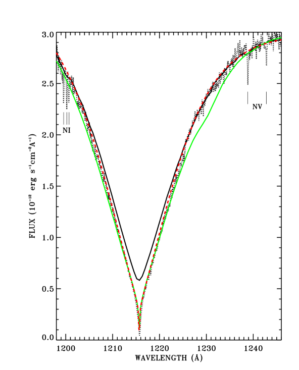
Another difference between the two NLTE results is the inclusion of quasi-molecular hydrogen lines in tlusty but not yet in the tmap code. These quasi-molecular features are most pronounced in the coolest star and their main impact lies below the 1150 Å STIS cutoff; however, a subtle flux depression appears at 1230 Å as illustrated for GD71 in Figure 7. Although there is some evidence for a much weaker G140L feature, which is slightly below the red tmap profile, the green tlusty feature is stronger than supported by the observations, which suggests that the tmap models are preferred at Ly. The G140M absorption line regions are masked for the G140L flux calibration. In Figure 7, the G140L line-core level is raised by 10% of the continuum level by stray light from the broad wings of the wide line-profile with the 522 slit; however, the narrow-slit (0.20.2), higher-resolution G140M line-core agrees remarkably well with the models. The region of contamination in the low-dispersion G140L line core is too wide for a successful spline fit between the unmasked wings; and the sensitivity must be estimated by linear interpolation between 1200 and 1230 Å for the tmap models. The extraneous tlusty quasi-molecular feature would require even more interpolation over 1200–1240Å.
In summary, the final set of models for the three primary standard stars includes the pure hydrogen tmap models for GD153 and GD71 that have no quasi-molecular hydrogen features in agreement with the observations. For G191-B2B, the tlusty model produces a more consistent flux calibration than the tmap model in the 2000-3900 Å range. This set of one tlusty and two tmap models forms the primary set of standard candles that is used for the flux calibration, which is defined by the average of the sensitivities from the comparably robust sets of STIS observations for each of the three primary standards. The sensitivities are the ratios of the observed signals to the reference SEDs which are defined by normalizing each model to its stellar flux F in the 25 Å band centered at 5557.5 Å (vac), where F = F(Vega) R. The ratio R is the relative brightness of each primary to Vega, as determined by the average STIS signal for each of the WD primaries divided by the STIS Vega signal in the same 25 Å band. F(Vega) = erg cm-2 s-1 Å-1 at 5557.5 Å (see the next Section). There is no dependence on the photometry for Vega or any of the primary standards, in contrast to the original normalization of the models using V-band photometry (Bohlin, 2000).
The STIS flux calibration observations all utilize the wide photometric 52x2 arcsec slit, but the point spread function (PSF) has extensive wings that bring contaminating continuum flux into the absorption line cores, especially for MAMA observations. Thus, the line cores are masked where the wavelength regions in Table 2 must be ignored in the derivation of the sensitivity vector, which is defined by a spline fit with a node spacing of 5 Å at the short wavelengths and 200 Å at the longest wavelengths.
| ID | Range (Å) |
|---|---|
| NIaaInterstellar/Circumstellar | 1198–1202.2 |
| Ly | 1209–1222 |
| NVaaInterstellar/Circumstellar | 1238–1239.6 |
| OIaaInterstellar/Circumstellar | 1300–1304.4 |
| CIIaaInterstellar/Circumstellar | 1332–1338 |
| CIVaaInterstellar/Circumstellar | 1547–1552 |
| MgIIaaInterstellar/Circumstellar | 2790–2810 |
| H | 3885–3905 |
| H | 3955–3990 |
| H | 4070–4140 |
| H | 4332–4352 |
| H | 4857–4870 |
| H | 6552–6577 |
| Pa | 9500–9600 |
| Pa | 10000–10100 |
Figure 8 illustrates the change in the HST/CALSPEC flux for each of the three primary WD standards. For a flux calibration that is based on equal weights for the three primary stars, the change in the flux calibration would be just the average of the three top panels. However, G191-B2B is too bright for the STIS pulse counting G140L and G230L MAMA detectors; and the STIS fluxes for these two modes are determined entirely by the pure hydrogen models for GD153 and GD71. G191-B2B can be used for all three CCD modes, which cover the 1670–10200 Å range. Thus, the average change in the bottom panel represents the average for all three stars above 1670 Å and for the two fainter stars below 1670 Å. These average changes that are due to changes in the reference WD models are 1% from 1670 Å to 10 µm.

As a final confirmation of the consistency of our three prime standards, Figure 9 shows that the ratio of the calibrated data to the chosen model flux has broadband residuals of 0.5% except in the hard-to-model confluence of the Balmer lines near 3800 Å for G191-B2B. These residuals are slightly improved in comparison to the previous pure tmap model set for the three primary standard WDs that is shown in figure 13 of Bohlin et al. (2019). Using Sloan spectroscopy and photometry, Allende Prieto et al. (2009) show a similar graph in their figure 8, where their broadband residuals sometimes approach 1.5% in the 3000–7000 Å range. Allende Prieto et al. (2009) have a different model grid, different assumptions about interstellar reddening, and a pure hydrogen model for the metal line-blanketed G191-B2B. However, our new self-consistent analysis demonstrates residuals generally 0.5% in the same wavelength range, with the exception of previously mentioned narrow bump near 3800 Å for G191-B2B.

3.1 Saturated CCD Data for Vega and Sirius
Historically, two of the brightest stars in the sky, Sirius and Vega, have been extensively observed for purposes of measuring their absolute flux distributions. STIS can observe these important stars in the well-calibrated CCD low-dispersion CCD modes G230LB, G430L, and G750L (Riley, 2019). Unfortunately, these standard stars are so bright that all the CCD data are saturated, except for Vega with G230LB and the shortest reliable exposure time. However, Gilliland (2004) demonstrated that the response is still linear to 0.1% for a factor of 50 overexposure, as long as all the saturated pixels are included in the spectral extractions height. At the gain=4 setting, the excess charge just bleeds into adjacent pixels along the columns, which are perpendicular to the dispersion axis. As detailed by Bohlin & Gilliland (2004) and Bohlin (2014), the net signal extracted with heights larger than the standard 11 pixels includes an extra fraction of the PSF, which must be removed before applying the standard flux calibration procedure. This extra signal is the ratio of the large height to the 11 pixel net signal derived from unsaturated observations of AGK+81∘266 in each of the CCD modes with correction for CTE losses in both heights. As proof of this procedure the unsaturated 0.9 s G230LB SEDs of Vega are compared to the flux derived from the saturated 18 s exposures in Figure 10. The short exposure fluxes agree with the long exposures to 0.23%. The wide extractions of the saturated data have such a large signal that the CTE correction is negligible; formally, the CTE correction formula of Goudfrooij et al. (2006) predicts 0.1% loss.
A previously unaccounted complication in defining the correction for the large extraction heights is that the spectral widths are increasing over time (Bohlin et al., 2019; Bohlin & Proffitt, 2015). Thus, the Vega corrections are the average of the 13 AGK+81∘266 observations within a year of the 2003.6 epoch of the Vega data, while more coverage in the timeframe of the Sirius data at the average 2012.9 date permits a window of 3 years. The uncertainty in these corrections for the large heights is estimated from the difference between the results for G230LB from the unsaturated Vega vs. AGK+81∘266, which range from 1.1% at 1720 Å to 0.6% at 3050 Å. Because the signal is the largest at 3050 Å and closer to the typical signal levels of G430L and G750L, perhaps, the 0.6% uncertainty is appropriate for the longer wavelengths.

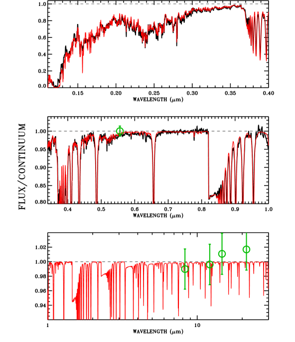
Figure 11 compares the STIS flux for Sirius to a R = 500 resolution Kurucz model. Below 1675 Å, an International Ultraviolet Explorer (IUE) spectrum completes the measured SED after normalization to the STIS flux by multiplying by 1.26. In order to display the spectral features on an expanded scale, the illustrated SEDs have been divided by the same theoretical smooth continuum. The model and the continuum are both normalized to the STIS flux in the line-free 6800–7700 Å continuum region, where the model should be the most reliable. Ratio plots of STIS/model have distracting, spurious dips and spikes near absorption line features because of small mismatches in resolution, tiny wavelength errors, and uncertain line strengths. The ratios of flux/continuum in Figure 11 display the nature of the absorption lines, and the irrelevant small mismatches at line centers are often off-scale and can be easily ignored. Many of the weaker STIS absorption lines have corresponding features in the Kurucz model, so the model replicates the measurements with high fidelity. Thus, longward of 1 µm, the 2013 Kurucz model (private communication), normalized to the STIS flux in the 6800–7700 Å range, is chosen for the composite CALSPEC SED for Sirius. In contrast to Vega with its unresolved dust ring, Sirius has no dust ring and this composite SED of STIS plus model should comprise a good fundamental standard reference spectrum to at least 30 µm. On the other hand, the Vega dust ring dominates the far-IR SED and prohibits the use of a photospheric model as an IR flux standard. The IR emission from the Vega dust contributes more than 1% to the photospheric flux longward of 2 µm, e.g., Bohlin (2014), so the CALSPEC photospheric model for Vega in the IR does not represent the true SED for unresolved observations of the total, photosphere plus dust disk.
Following the logic of Bohlin (2014), the four green circles in the IR in Figure 11 are the ratio of the MSX results of (Price et al., 2004) to the Sirius model, which is normalized to the STIS SED that uses the original Megessier (1995) Vega flux of erg cm-2 s-1 Å-1 at 5557.5 Å (vac) to set the absolute CALSPEC flux scale. The average MSX ratio is 1.0034, in contrast to the previous value of 0.989 (Bohlin, 2014). With a unit ratio at 5557.5 Å for the original CALSPEC absolute flux zero point, the average of the visible and IR absolute flux ratios is 1.0017 too high; thus, the CALSPEC fluxes must all be increased by this factor to reconcile the two sets of preferred absolute flux measures that have the same weight. Equivalently, the CALSPEC absolute flux levels are set by increasing the Megessier (1995) value to erg cm-2 s-1 Å-1 at 5557.5 Å (vac, 5556 Å air), which happens to agree exactly with Tüg et al. (1977). The formal uncertainty is 0.5% in the average from combining the Megessier uncertainty of 0.7% with the total uncertainty of 0.7% for the set of four MSX points. This new absolute level for Vega replaces the previous erg cm-2 s-1 Å-1 of Bohlin (2014). This gray increase of 0.87% (3.47/3.44) in all the CALSPEC fluxes is in addition to the wavelength-dependent changes in Figure 8 that are due to improved WD model SEDs.
3.2 CALSPEC vs. Tüg et al. (1977) Absolute Flux Measures
Now that 109 Vir has been observed by STIS, the CALSPEC fluxes can be compared to the absolute flux determinations for both Vega and 109 Vir in Tüg et al. (1977). Figure 12 shows the ratio of the Tüg et al. (1977) results to the CALSPEC alpha_lyr_stis_010.fits and 109vir_stis_002.fits SEDs. Tüg et al. (1977) cover the 3295–9040 Å region with 10 Å bandpasses at the shorter wavelengths and 20 Å bandpasses at the longer wavelengths. In general, Tüg et al. (1977) measure at continuum wavelength sample points that avoid the confusion of absorption lines. However, that policy was enforced only at wavelengths below 8500 Å, which invalidates the ratios in the Paschen line region where resolution differences and tiny wavelength errors cause excess noise. Thus, Figure 12 shows only the valid 3295–8500 Å region with the average ratio and rms written on the plots. The ratios and rms are roughly consistent with the Tüg et al. (1977) uncertainty of 1% longward of 4000 Å, where most of the points are within 2 of unity, and only the one point for Vega at 5890 Å deviates by as much as 4. The two independent sets of absolute fluxes agree better than the comparison of CALSPEC with Hayes (1985) in the visible or with comparisons in the ultraviolet that are all shown in Bohlin et al. (2014). None of these comparisons show evidence of systematic CALSPEC flux errors.

4 Fitting Pure Hydrogen Models to STIS Observations
Following the Bohlin et al. (2014) and Bohlin & Deustua (2019) reduced method of fitting K to O type stars, WD SEDs are fit using the new tlusty207 and tmap2019 pure hydrogen grids discussed in Section 2. The extrapolated SEDs from the 1 µm STIS long-wavelength cutoff to 32 µm serve as reference flux distributions for IR flux calibration with a firm HST anchor at the shorter wavelengths. Any HST IR grism spectrophotometry that reaches to the Wide Field Camera 3 (WFC3) 1.7 µm limit or to the Near Infrared Camera and Multi-Object Spectrograph (NICMOS) 2.5 µm limit increases the lever arm of the extrapolation and decreases uncertainties. Both the WFC3 and NICMOS grism flux calibrations have been revised using the new SEDs for the three primary standards. The parameters of the best reduced fits are , , and E(B-V) for each modeled WD, as listed in Table 3. The maximum residual difference between the model fits and the data for the hotter stars does not exceed 1.6% in broad bins, except for SDSSJ151421, where the maximum residual is 2.5% in the 3300–3700 Å bin. The CALSPEC WD SEDs concatenate the measurements with the model fits at the longer wavelengths.
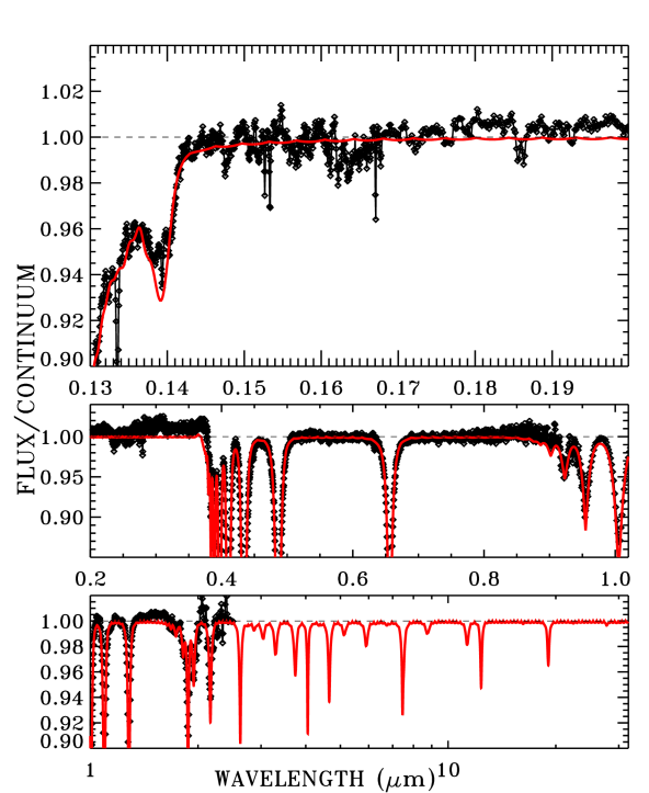
As an example of the utility of models that include quasi-molecular satellites (QMS), Figure 13 compares the strong observed QSM feature at 1400 Å to the tlusty model for the cool WD GRW+70∘5824. Despite confusion by absorption from the Si IV ground state at 1393.8 and 1402.8 Å, the tlusty model illustrates the nature of the QMS. While there are metal lines that could invalidate the fit, the model approximates the observed SED within 2% longward of 1300 Å. However, the metal-line features, the broad hydrogen lines, and the small systematic deviations of the model from the CALSPEC SED grw_70d5824_stiswfcnic_002.fits suggest that the model for GRW+70∘5824 does not make an ideal standard star. However, the observed SED grw_70d5824_stiswfcnic_002.fits is one of the best CALSPEC standards.
| Star | E(B-V) | |||
|---|---|---|---|---|
| GRW+70∘5824aaWFC3 and NICMOS grism data extend the observed SED longward of 1 µm. | 20540 | 7.90 | 0.000 | 0.05 |
| SDSSJ151421 | 29120 | 8.90 | 0.043 | 0.64 |
| WD0320-539 | 33110 | 7.60 | 0.000 | 0.10 |
| WD0947+857 | 40020 | 7.55 | 0.000 | 0.25 |
| WD1026+453 | 35240 | 7.55 | 0.000 | 0.20 |
| WD1657+343aaWFC3 and NICMOS grism data extend the observed SED longward of 1 µm. | 46750 | 7.10 | 0.000 | 0.10 |
Note. — Results from fitting model atmospheres to the observed stellar SEDs using fitting with the tmap pure hydrogen grid, except for GRW+70∘5824, which is fit with the tlusty grid. The parameters of the fit for each star are the effective temperature , the surface gravity , the interstellar reddening E(B-V), and the reduced chi-square quality of the fit .
4.1 CALSPEC vs. Narayan et al. (2019)
Narayan et al. (2019) and Calamida et al. (2019) have produced an all-sky network of faint WD absolute flux standards that are tied to the CALSPEC absolute flux scale by fitting F275W, F336W, F475W, F625W, F775W, and F160W filter photometry from the WFC3 on HST. One star SDSSJ151421.27+004752.8 in the network is bright enough at V = 16.5 to obtain fair S/N with STIS in two orbits and was observed 24 April 2019. The best fit to the STIS SED from Table 3 is a model with =29120 K, =8.90, and E(B-V)=0.043 for a calibration based on the new set of three primary flux standards. However, to make a fair comparison with Narayan et al. (2019), who based results on the previous system, a fit of the old SED for SDSSJ151421 grw_70d5824_stiswfcnic_001.fits is used for Figure 14 with its fit at =29010 K, =8.85, and E(B-V)=0.043. Figure 14 compares this old SED to the Narayan et al. (2019) fit of =28768 K, =7.89, and E(B-V)=0.039. Differences in these model labels are inconsequential; the important difference is between the pure hydrogen model flux distributions that are proposed as standard reference SEDs, as illustrated in Figure 14. The old STIS SED (black diamonds with 2 error bars), its tmap2019 model (red), and the Narayan et al. (2019) model (green) are all divided by the tmap2019 reddened continuum. In order to show the main spectral features, including the 2200 Å extinction bump, the reddened continuum is interpolated linearly across the 1800–2600 Å range, revealing a 15% dip at 2200 in the red model fit. The STIS observation is binned into statistically independent bins of 60 pixels and the error-in-the-mean is computed from the rms scatter among the 60 samples in each of bins. These error bars computed from the data are typically 2–4 times larger than the propagated statistical errors from the Poisson statistics.
The data are convincingly lower than the red model fit by 2–3% at 2200–3800 Å, where the measures agree well with the green fit but suggest that the reddening is anomalously larger than the average reddening used for the red model. These small deviations of the STIS SED from its red model are caused in part, or maybe in full, by typical variations from the Cardelli et al. (1989) average reddening assumed in the fitting process. Using other average reddening curves such as Fitzpatrick (1999) does not significantly change the results. For illustrations of the range of individual interstellar extinction curves, see Witt et al. (1984).
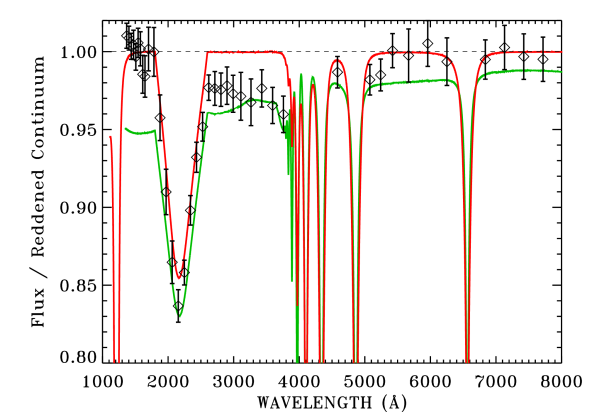
At wavelength longer than 5000 Å, the systematically larger STIS flux in all ten independent bins suggests that the green Narayan et al. (2019) fit is 1–2% low, which is a bit surprising, as the Narayan et al. (2019) fit is well constrained by WFC3 photometry in that wavelength region. Possibilities for the general trend of the green curve to fall below the red are errors in the STIS spectrophotometry of the faint SDSSJ151421.27+004752.8 and problems in accurately placing the WFC3 photometry on the CALSPEC scale, including small errors in the lab measurements of the filter throughput curves. Bohlin (2016) found that some ACS filter curves required significant changes in order to achieve a 1% photometry goal. The STIS observations of SDSSJ151421 should be repeated to confirm the single measurement for such a faint star.
In summary, the Narayan et al. (2019) results are confirmed in the region where there are WFC3 constraints at the F275W filter and longward, but only to a precision of 2%, rather than to the goal of 1%. At FUV wavelengths in the unconstrained 1500 Å region, the fit of Narayan et al. (2019) is too low by 5%.
Other differences between the red and green curves in Figure 14 include the use of an earlier version of the tlusty grid, rather than the new tmap2019 grid recommended here. For the best absolute fluxes of the all-sky network of faint WDs, a new analysis should include a recalibration of the WFC3 photometry using the three revised primary WD flux standards, followed by a re-fitting of that recalibrated WFC3 photometry with the new tmap2019 grid. The uncertainties associated with anomalous reddening curves in the UV and small filter bandpass shifts should also be quantified.
5 Summary
Because of the changes in the SEDs of the three primary standards, all of the HST flux calibrations must be updated to achieve the goal of 1% precision.. The recalibration of the five STIS low dispersion modes and the WFC3 and NICMOS IR grisms is complete, and the 99 stars in the CALSPEC database with STIS, WFC3, or NICMOS observations are re-delivered. In addition, models for 73 of the 99 stars are included in the update. No models are available for the three stars with observations of NICMOS only, for five M, T, or L type stars, or for the stars with partial STIS coverage in table 1b of CALSPEC. The remaining 16 stars with no model include cases where there is a dust ring that affects the SED in the IR, where the WD is too cool or is not pure hydrogen, where the star is variable, or where there is a close companion that affects the measured SED. The model files for the main-sequence stars are the R=300,000 BOSZ models of Bohlin et al. (2017), while the R=500 BOSZ version is concatenated to the observed SED at the long wavelengths of the CALSPEC data files. The concatenated portion of the WD data files is the same as in the model WD files.
The changes in flux for the updated SEDs often do not correspond exactly to the average change in Figure 8 plus the 0.87% gray increase of Section 3.1, because of the non-uniform processing dates of the replaced files. Other smaller changes occured over time, e.g., increasing the extraction width from 7 to 11 pixels for the CCD data and updating the correction for sensitivity changes over time, etc. (Bohlin et al., 2019).
The new WD pure hydrogen grids are available in the MAST Archive via https://doi.org/10.17909/t9-7myn-4y46 (catalog https://doi.org/10.17909/t9-7myn-4y46) .
Acknowledgements
Support for this work was provided by NASA through the Space Telescope Science Institute, which is operated by AURA, Inc., under NASA contract NAS5-26555. Thanks to Abi Saha for inspiring this paper. His team has established a network of faint WD spectrophotometric flux standards, and the team members are the author lists of Narayan et al. (2019) and Calamida et al. (2019).
ORCID IDs
Ralph C. Bohlin https://orcid.org/0000-0001-9806-0551
Ivan Hubeny https://orcid.org/0000-0001-8816-236X
Thomas Rauch https://orcid.org/0000-0003-1081-0720
References
- Allard et al. (1994) Allard, N. F., Koester, D., Feautrier, N., & Spielfiedel, A. 1994, A&AS, 108, 417
- Allende Prieto et al. (2009) Allende Prieto, C., Hubeny, I., & Smith, J. A. 2009, MNRAS, 396, 759
- Bohlin (2000) Bohlin, R. C. 2000, The Astronomical Journal, 120, 437
- Bohlin (2014) Bohlin, R. C. 2014, AJ, 147, 127
- Bohlin (2016) —. 2016, AJ, 152, 60
- Bohlin & Deustua (2019) Bohlin, R. C., & Deustua, S. E. 2019, AJ, 157, 229
- Bohlin et al. (2019) Bohlin, R. C., Deustua, S. E., & de Rosa, G. 2019, The Astronomical Journal, 158, 211
- Bohlin & Gilliland (2004) Bohlin, R. C., & Gilliland, R. L. 2004, AJ, 127, 3508
- Bohlin et al. (2014) Bohlin, R. C., Gordon, K. D., & Tremblay, P.-E. 2014, PASP, 126, 711
- Bohlin & Landolt (2015) Bohlin, R. C., & Landolt, A. U. 2015, AJ, 149, 122
- Bohlin et al. (2017) Bohlin, R. C., Mészáros, S., Fleming, S. W., et al. 2017, AJ, 153, 234
- Bohlin & Proffitt (2015) Bohlin, R. C., & Proffitt, C. R. 2015, Improved Photometry for G750L, Instrument Science Report, STIS 2015–01, (Baltimore: STScI), Tech. rep.
- Bohlin et al. (1978) Bohlin, R. C., Savage, B. D., & Drake, J. F. 1978, ApJ, 224, 132
- Calamida et al. (2019) Calamida, A., Matheson, T., Saha, A., et al. 2019, ApJ, 872, 199
- Cardelli et al. (1989) Cardelli, J. A., Clayton, G. C., & Mathis, J. S. 1989, ApJ, 345, 245
- Dupuis et al. (1995) Dupuis, J., Vennes, S., Bowyer, S., Pradhan, A. K., & Thejll, P. 1995, ApJ, 455, 574
- Fitzpatrick (1999) Fitzpatrick, E. L. 1999, PASP, 111, 63
- Gentile Fusillo et al. (2020) Gentile Fusillo, N. P., Tremblay, P.-E., Bohlin, R. C., Deustua, S. E., & Kalirai, J. S. 2020, MNRAS, 491, 3613
- Gianninas et al. (2011) Gianninas, A., Bergeron, P., & Ruiz, M. T. 2011, ApJ, 743, 138
- Gilliland (2004) Gilliland, R. L. 2004, ACS CCD Gains, Full Well Depths, and Linearity up to and Beyond Saturation, Instrument Science Report ACS 2004–01, (Baltimore: STScI), Tech. rep.
- Goudfrooij et al. (2006) Goudfrooij, P., Bohlin, R. C., Maíz-Apellániz, J., & Kimble, R. A. 2006, PASP, 118, 1455
- Hayes (1985) Hayes, D. S. 1985, in IAU Symposium, Vol. 111, Calibration of Fundamental Stellar Quantities, ed. D. S. Hayes, L. E. Pasinetti, & A. G. D. Philip (Dordrecht: Reidel), 225
- Hubeny et al. (1994) Hubeny, I., Hummer, D. G., & Lanz, T. 1994, A&A, 282, 151
- Hubeny & Lanz (1995) Hubeny, I., & Lanz, T. 1995, ApJ, 439, 875
- Hubeny & Lanz (2017a) —. 2017a, arXiv e-prints, arXiv:1706.01859
- Hubeny & Lanz (2017b) —. 2017b, arXiv e-prints, arXiv:1706.01935
- Hubeny & Mihalas (2014) Hubeny, I., & Mihalas, D. 2014, Theory of Stellar Atmospheres, Princeton Univ. Pres
- Koornneef & Code (1981) Koornneef, J., & Code, A. D. 1981, ApJ, 247, 860
- Kurucz (1970) Kurucz, R. L. 1970, SAO Special Report, 309
- Landolt (1992) Landolt, A. U. 1992, AJ, 104, 340
- Landolt & Uomoto (2007) Landolt, A. U., & Uomoto, A. K. 2007, AJ, 133, 768
- Lanz & Hubeny (2003) Lanz, T., & Hubeny, I. 2003, ApJS, 146, 417
- Lanz & Hubeny (2007) —. 2007, ApJS, 169, 83
- Megessier (1995) Megessier, C. 1995, A&A, 296, 771
- Narayan et al. (2019) Narayan, G., Matheson, T., Saha, A., et al. 2019, ApJS, 241, 20
- Price et al. (2004) Price, S. D., Paxson, C., Engelke, C., & Murdock, T. L. 2004, AJ, 128, 889
- Rauch (2008) Rauch, T. 2008, A&A, 481, 807
- Rauch & Deetjen (2003) Rauch, T., & Deetjen, J. L. 2003, in Astronomical Society of the Pacific Conference Series, Vol. 288, Stellar Atmosphere Modeling, ed. I. Hubeny, D. Mihalas, & K. Werner, 103
- Rauch et al. (2013) Rauch, T., Werner, K., Bohlin, R., & Kruk, J. W. 2013, A&A, 560, A106
- Riley (2019) Riley, A. 2019, STIS Instrument Handbook, Version 18.0, (Baltimore:STScI)
- Tremblay & Bergeron (2009) Tremblay, P.-E., & Bergeron, P. 2009, ApJ, 696, 1755
- Tremblay & Bergeron (2010) Tremblay, P. E., & Bergeron, P. 2010, in American Institute of Physics Conference Series, ed. K. Werner & T. Rauch, Vol. 1273, 1–6
- Tüg et al. (1977) Tüg, H., White, N. M., & Lockwood, G. W. 1977, A&A, 61, 679
- Werner et al. (2003) Werner, K., Deetjen, J. L., Dreizler, S., et al. 2003, in Astronomical Society of the Pacific Conference Series, Vol. 288, Stellar Atmosphere Modeling, ed. I. Hubeny, D. Mihalas, & K. Werner, 31
- Werner et al. (2012) Werner, K., Dreizler, S., & Rauch, T. 2012, TMAP: Tübingen NLTE Model-Atmosphere Package, Astrophysics Source Code Library [record ascl:1212.015], ascl:1212.015
- Witt et al. (1984) Witt, A. N., Bohlin, R. C., & Stecher, T. P. 1984, ApJ, 279, 698