A Mathematical Analysis of Mathematical Faculty

Abstract

We use the data of tenured and tenure-track faculty at ten public and private math departments of various tiered rankings in the United States, as a case study to demonstrate the statistical and mathematical relationships among several variables, e.g., the number of publications and citations, the rank of professorship and AMS fellow status. At first we do an exploratory data analysis of the math departments. Then various statistical tools, including regression, artificial neural network, and unsupervised learning, are applied and the results obtained from different methods are compared. We conclude that with more advanced models, it may be possible to design an automatic promotion algorithm that has the potential to be fairer, more efficient and more consistent than human approach.

1 Introduction

Modern research universities and colleges around the globe employ tenure track and tenured professors in STEM fields in a large part for the quality and impact of the research they produce. However, the process of promotion on this tenure track is inefficient, time-consuming, and varies from institution to institution. It is largely based on subjective evaluations by “experts”, and endless committee meetings, with many steps along the way where personal bias may undermine a promising candidate. As such, an algorithmic approach to promotion may be a vast improvement to the current system. The purpose of this paper is to determine whether or not this is feasible, by testing if automated algorithms can predict the rank of tenure track professors in public and private universities in the United States. As the authors are from a department of mathematics and are most familiar with mathematical academia, we concentrate on math departments.

The variables considered in the development of a promotion algorithm for mathematics are: years from PhD, number of papers, number of citations, h-index, and AMS Fellowship status. We attempt to predict if a candidate is an associate professor, assistant professor, professor, or distinguished professor from this, using tools of regression, artificial neural network and unsupervised learning to the data set we collected for predictive exploration. We discover (perhaps unsurprisingly) that there are very strong statistical properties shared within certain groups of ranks. We conclude this means that an unbiased algorithm could be built by studying data and finding patterns to avoid subjective opinions and maintain consistent standards. It is important to note that while race and gender of the candidates was beyond the scope of this study, instituting an algorithmic approach to promotion may also help mitigate negative bias with regards to race or gender in academic promotions.

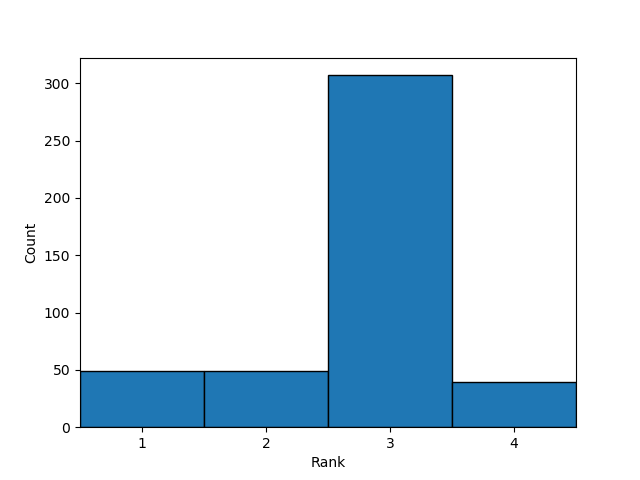
For this paper, we collect public data online of the tenured and tenure-track faculty members at math departments of 10 universities: UC Berkeley, Dartmouth College, University of Florida, Harvard University, University of Michigan, Massachusetts Institute of Technology, University of Pennsylvania, Princeton University, Rutgers University-New Brunswick and UCLA. In our data set, totally there are 444 professors. The variables are Lastname, Firstname, Rank (Assistant Professor=1, Associate Professor=2, Full Professor=3, Distinguished Professor=4), Number of Publication, Number of Citations, $h$-Index, AMS Fellow (Yes=1, No=0), the Year of Ph.D. Awarded.

The data of names and ranks are from the website of each math department. Note that some departments, e.g., Princeton and Harvard, do not have the rank of Distinguished Professor. The numbers of publications, citations and $h$-index are from MathSciNet. It is worth emphasizing that MathSciNet has much more strict standards for recording publications, citations and $h$-index so that the MathSciNet $h$-index is much lower (roughly a half) from that which can be found using Google Scholar. AMS membership was taken from the AMS website. Year of attaining the rank of PhD was taken from Mathematics Genealogy. All data was collected in or around November 2019.

2 Exploratory Data Analysis

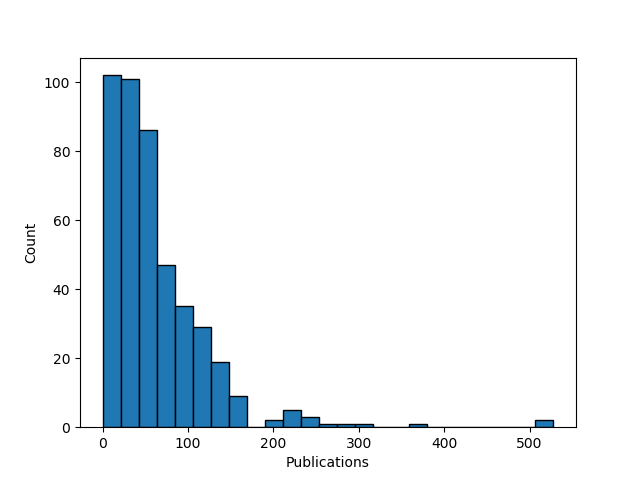
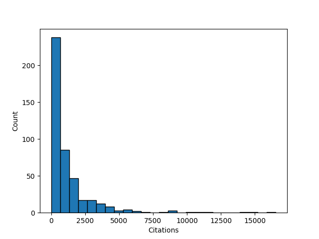
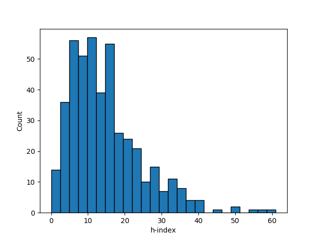
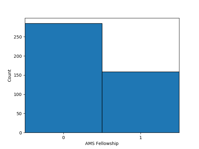
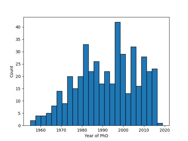
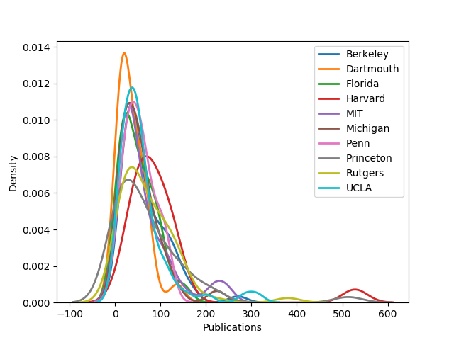
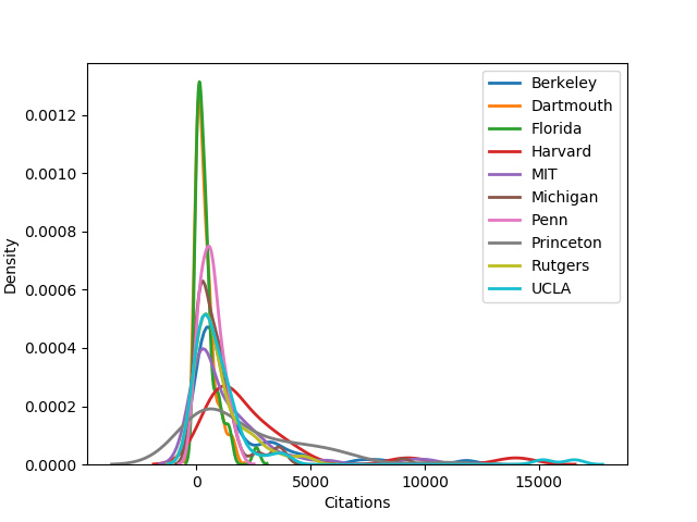
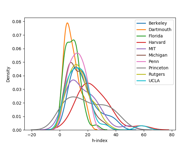
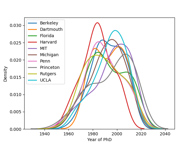
The following three charts show the means and the standard deviations for each of the fields considered across all universities.

Field	Mean	Standard Deviation
Rank	2.757	0.763
Number of Publications	62.459	60.063
Number of Citations	1250.153	2012.400
h-index	14.777	9.866
AMS Fellowship	0.358	0.480
Year of PhD	1992.304	14.538

Table 1: Means and standard deviations across all universities (n=444)

University	n	Rank	Publications	Citations	h-index	AMS Fellowship	Year of PhD
Berkeley	58	2.741	64.914	1579.017	17.207	0.362	1992.776
Dartmouth	23	2.478	36.783	360.435	8.652	0.043	1993.652
Florida	44	2.500	50.568	416.477	9.136	0.045	1992.091
Harvard	20	3.000	100.400	2810.800	24.500	0.400	1984.000
MIT	53	2.642	63.491	1460.094	16.377	0.415	1995.717
Michigan	62	2.871	54.258	936.742	12.887	0.339	1991.694
Penn	25	2.800	53.960	633.200	12.320	0.400	1989.440
Princeton	42	2.452	73.524	2123.738	19.357	0.452	1995.071
Rutgers	59	3.153	71.661	1027.525	14.271	0.559	1989.051
UCLA	58	2.776	60.241	1371.379	14.517	0.379	1994.397

Table 2: Means across all universities, by university (n=444)

University	n	Rank	Publications	Citations	h-index	AMS Fellowship	Year of PhD
Berkeley	58	0.609	48.665	2174.119	9.472	0.485	12.445
Dartmouth	23	0.790	30.705	399.379	4.914	0.209	12.463
Florida	44	0.876	37.279	507.301	5.129	0.211	15.397
Harvard	20	0.000	106.460	3291.795	11.390	0.503	12.645
MIT	53	0.787	59.765	2083.936	10.895	0.497	15.468
Michigan	62	0.614	45.168	1364.324	7.378	0.477	13.745
Penn	25	0.645	31.798	465.785	5.429	0.500	14.509
Princeton	42	0.889	90.541	2465.433	13.483	0.504	17.374
Rutgers	59	0.979	62.757	1128.886	7.850	0.501	15.234
UCLA	58	0.531	59.434	2898.606	10.881	0.489	13.124

Table 3: Standard deviations across all universities, by university (n=444)

Out of the mathematics departments in the study, Harvard led in the averages for number of publications, number of citations, the h-index, and number of years since Ph.D., followed in each of these metrics except for the last by Princeton, whose faculty on average completed their doctorates a full eleven years after their Harvard colleagues. Princeton also had the greatest variation in the $h$-index and the academic age of its faculty; however, this may result from a different classification system used by Princeton that does not award full tenure. Rutgers led in both the average rank of the faculty titles and the proportion of AMS Fellows, despite being slightly below average in both the number of citations and the h-index.

Dartmouth, Florida, and Penn had the lowest variability among its faculty in the number of publications, number of citations, and the h-index.

The following charts show the extrapolated percentiles for each field:

	Percentiles
Field	5	10	25	50	75	90	95
Rank	2	2	3	3	3	3	3
Publications	11	14	25	44	71	111	164
Citations	30	68	208	626	1392	2260	3750
h-index	4	4	8	13	18	22	31
AMS Fellowship	0	0	0	0	1	1	1
Year of PhD	1970	1977	1986	1996	2006	2009	2012

Table 4: Percentiles for all fields across all universities (n=444)

	Percentiles
University	5	10	25	50	75	90	95
Berkeley	1	2	3	3	3	3	3
Dartmouth	1	1	2	3	3	3	3
Florida	1	1	2	3	3	3	4
Harvard	3	3	3	3	3	3	3
MIT	1	1	3	3	3	3	3
Michigan	2	2	3	3	3	3	4
Penn	1	2	3	3	3	3	3
Princeton	1	1	1	3	3	3	3
Rutgers	1	2	3	3	4	4	4
UCLA	2	2	3	3	3	3	3

Table 5: Percentiles for professor rank across all universities, by university (n=444)

	Percentiles
University	5	10	25	50	75	90	95
Berkeley	18	23	30	43	88	131	139
Dartmouth	9	9	14	26	58	65	75
Florida	8	11	19	42	76	98	106
Harvard	38	39	48	74	112	137	158
MIT	13	14	26	40	81	133	215
Michigan	10	13	21	45	70	100	122
Penn	11	18	28	54	75	103	110
Princeton	3	6	10	53	94	160	207
Rutgers	10	15	26	58	104	138	155
UCLA	11	14	25	44	71	111	164

Table 6: Percentiles for number of publications across all universities, by university (n=444)

	Percentiles
University	5	10	25	50	75	90	95
Berkeley	188	210	366	718	1786	3800	5320
Dartmouth	35	38	72	167	510	918	1086
Florida	30	33	70	261	488	965	1361
Harvard	743	754	990	1440	3000	4862	9490
MIT	28	52	165	622	1683	3194	4968
Michigan	31	76	184	602	1087	1759	3501
Penn	56	99	241	586	927	1285	1379
Princeton	9	37	142	1158	3664	5732	6260
Rutgers	38	75	209	632	1446	2536	3500
UCLA	30	68	208	626	1392	2260	3750

Table 7: Percentiles for number of citations across all universities, by university (n=444)

	Percentiles
University	5	10	25	50	75	90	95
Berkeley	7	8	9	15	22	33	36
Dartmouth	3	3	5	8	11	16	18
Florida	3	3	4	9	12	16	17
Harvard	14	14	17	22	32	35	39
MIT	3	6	9	13	23	29	34
Michigan	3	4	8	12	17	23	26
Penn	5	5	8	12	16	20	20
Princeton	2	4	6	16	31	39	41
Rutgers	4	5	8	13	18	26	27
UCLA	4	4	8	13	18	22	31

Table 8: Percentiles for the h-index across all universities, by university (n=444)

	Percentiles
University	5	10	25	50	75	90	95
Berkeley	1973	1975	1984	1992	2002	2010	2011
Dartmouth	1979	1979	1982	1996	2004	2010	2012
Florida	1969	1973	1982	1988	2006	2013	2014
Harvard	1966	1967	1978	1984	1991	2000	2004
MIT	1966	1974	1988	1997	2008	2013	2014
Michigan	1967	1971	1983	1994	2002	2009	2011
Penn	1965	1976	1980	1987	2002	2009	2012
Princeton	1966	1973	1980	2000	2011	2014	2015
Rutgers	1968	1969	1977	1989	2000	2011	2014
UCLA	1970	1977	1986	1996	2006	2009	2012

Table 9: Percentiles for year of PhD across all universities, by university (n=444)

The covariance and correlation matrices follow:

	Rank	Publications	Citations	h-index	AMS Fellowship	Year of PhD
Rank	0.582	19.624	437.279	3.485	0.151	-7.125
Publications	19.624	3607.558	94206.857	473.972	10.600	-461.266
Citations	437.279	94206.857	4049753.638	17365.165	352.855	-12455.609
h-index	3.485	473.972	17365.165	97.338	2.166	-73.794
AMS Fellowship	0.151	10.600	352.855	2.166	0.230	-2.617
Year of PhD	-7.125	-461.266	-12455.609	-73.794	-2.617	211.359

Table 10: The covariance matrix for all universities (n=444)

	Rank	Publications	Citations	h-index	AMS Fellowship	Year of PhD
Rank	1.000	0.428	0.285	0.463	0.411	-0.642
Publications	0.428	1.000	0.779	0.800	0.368	-0.528
Citations	0.285	0.779	1.000	0.875	0.365	-0.426
h-index	0.463	0.800	0.875	1.000	0.457	-0.514
AMS Fellowship	0.411	0.368	0.365	0.457	1.000	-0.375
Year of PhD	-0.642	-0.528	-0.426	-0.514	-0.375	1.000

Table 11: The correlation matrix for all universities (n=444)

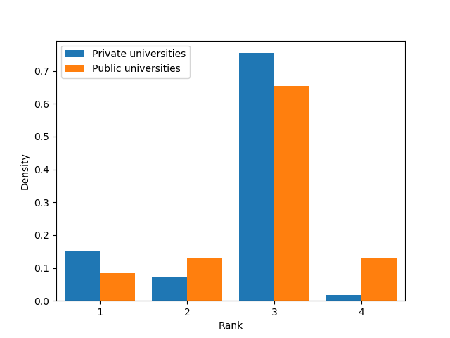
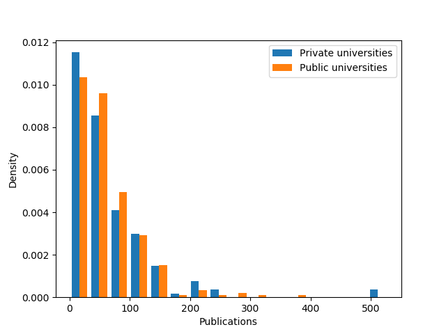
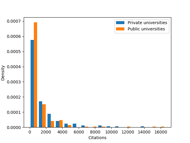
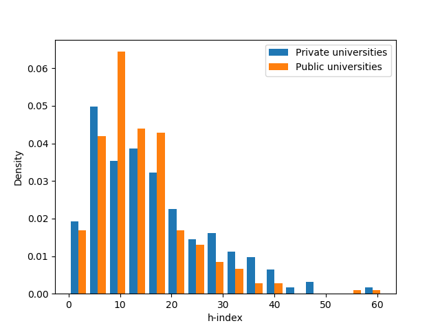
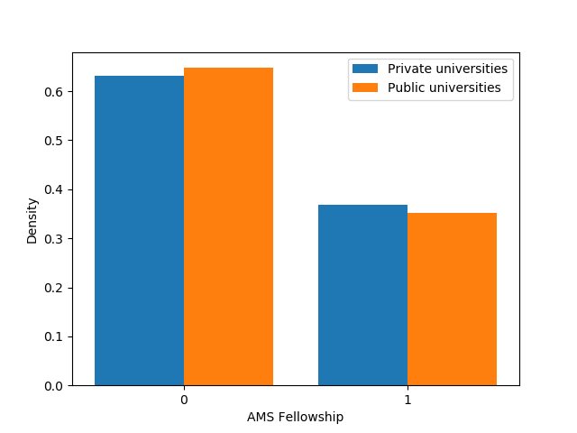
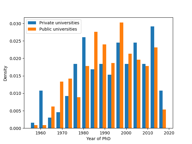
Dividing the universities surveyed into two groups depending on whether they are private or public, we have the following comparisons:

Field	Mean	Standard Deviation
Rank	2.638	0.760
Number of Publications	65.374	71.654
Number of Citations	1514.834	2206.948
h-index	16.429	11.333
AMS Fellowship	0.368	0.484
Year of PhD	1992.859	15.484

Table 12: Means and standard deviations across private universities (n=163)

Field	Mean	Standard Deviation
Rank	2.826	0.757
Number of Publications	60.769	52.242
Number of Citations	1096.619	1877.458
h-index	13.819	8.785
AMS Fellowship	0.352	0.479
Year of PhD	1991.982	13.979

Table 13: Means and standard deviations across public universities (n=281)

	Rank	Publications	Citations	h-index	AMS Fellowship	Year of PhD
Rank	0.578	19.815	535.983	4.200	0.146	-7.379
Publications	19.815	5134.347	139945.667	664.980	12.923	-586.052
Citations	535.983	139945.667	4870620.497	22485.337	377.932	-17699.863
h-index	4.200	664.980	22485.337	128.432	2.390	-103.130
AMS Fellowship	0.146	12.923	377.932	2.390	0.234	-3.090
Year of PhD	-7.379	-586.052	-17699.863	-103.130	-3.090	239.752

Table 14: The covariance matrix for private universities (n=163)

	Rank	Publications	Citations	h-index	AMS Fellowship	Year of PhD
Rank	0.573	19.902	410.637	3.265	0.155	-6.942
Publications	19.902	2729.271	67370.508	360.722	9.268	-392.204
Citations	410.637	67370.508	3524847.394	14062.499	337.174	-9601.000
h-index	3.265	360.722	14062.499	77.185	2.028	-57.928
AMS Fellowship	0.155	9.268	337.174	2.028	0.229	-2.358
Year of PhD	-6.942	-392.204	-9601.000	-57.928	-2.358	195.403

Table 15: The covariance matrix for public universities (n=281)

	Rank	Publications	Citations	h-index	AMS Fellowship	Year of PhD
Rank	1.000	0.364	0.319	0.487	0.398	-0.627
Publications	0.364	1.000	0.885	0.819	0.373	-0.528
Citations	0.319	0.885	1.000	0.899	0.354	-0.518
h-index	0.487	0.819	0.899	1.000	0.436	-0.588
AMS Fellowship	0.398	0.373	0.354	0.436	1.000	-0.412
Year of PhD	-0.627	-0.528	-0.518	-0.588	-0.412	1.000

Table 16: The correlation matrix for private universities (n=163)

	Rank	Publications	Citations	h-index	AMS Fellowship	Year of PhD
Rank	1.000	0.503	0.289	0.491	0.427	-0.656
Publications	0.503	1.000	0.687	0.786	0.371	-0.537
Citations	0.289	0.687	1.000	0.853	0.375	-0.366
h-index	0.491	0.786	0.853	1.000	0.482	-0.472
AMS Fellowship	0.427	0.371	0.375	0.482	1.000	-0.352
Year of PhD	-0.656	-0.537	-0.366	-0.472	-0.352	1.000

Table 17: The correlation matrix for public universities (n=281)

The correlation matrices were largely similar between the private and public universities studied, with three notable exceptions:

• The correlation between the faculty rank and the number of publications was much stronger for public universities (0.503) than for private universities (0.364).

• The correlation between the number of publications and the number of citations was much stronger for private universities (0.885) than for public universities (0.687).

• The correlation between the academic age and the number of citations was much stronger for private universities (-0.518) than for public universities (-0.366).

Figure 1: Histograms for each data field across all universities (n=444)

Figure 2: Normalized histograms for each data field across all private and public universities (n=444)

Figure 3: Kernel density estimates for each data field across each university (n=444)

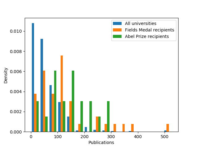
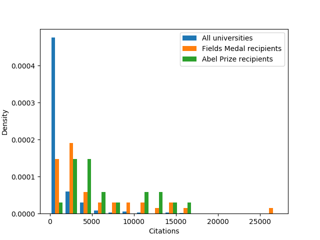
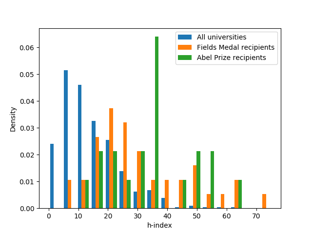
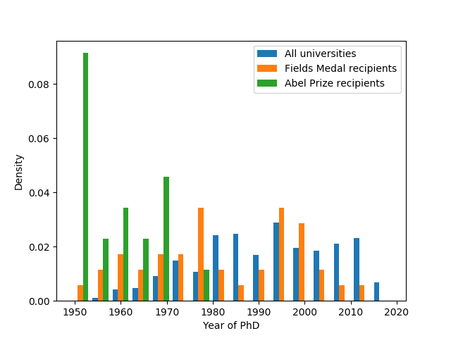
We further analyzed the data for living Fields medalists as well as all Abel Prize recipients.

Field	Mean	Standard Deviation
Number of Publications	130.300	110.607
Number of Citations	5201.800	5663.499
h-index	31.050	16.399
Year of PhD	1982.175	16.522

Table 18: Means and standard deviations across Fields medalists (n=40)

Field	Mean	Standard Deviation
Number of Publications	142.300	75.385
Number of Citations	6687.050	4538.117
h-index	34.600	14.095
Year of PhD	1958.450	8.988

Table 19: Means and standard deviations across Abel Prize recipients (n=20)

	Publications	Citations	h-index	Year of PhD
Publications	1.000	0.777	0.807	-0.397
Citations	0.777	1.000	0.946	-0.413
h-index	0.807	0.946	1.000	-0.491
Year of PhD	-0.397	-0.413	-0.491	1.000

Table 20: The correlation matrix for Fields medalists (n=40)

	Publications	Citations	h-index	Year of PhD
Publications	1.000	0.573	0.705	-0.177
Citations	0.573	1.000	0.944	-0.213
h-index	0.705	0.944	1.000	-0.193
Year of PhD	-0.177	-0.213	-0.193	1.000

Table 21: The correlation matrix for Abel Prize recipients (n=20)

Figure 4: Normalized histograms for each data field comparing university professors (n=444) to Fields medalists (n=40) and Abel Prize reciepients (n=20)

3 Regression Method to Predict Rank and AMS-fellowship

In this section a regression method is used to attempt to predict the rank and AMS-fellow status from Number of publications, number of citations, h-index and year of PhD. However, we cannot apply these regression method directly, since the results are discrete. Specifically, our ranking goal can be regarded as a classification problem. Regression methods are often highly successful with binary classification problems. However, when we come to a multi-states classification problem, such as the four ranks we wish to predict, it seems less obvious to use these methods (except perhaps the logistic regression method). Therefore, we will make some changes on these regression method to make them can be applied on multi-classification problem. Section 3.1 details the regression method that we use. The rest of the section applies this methodology to predict rank and AMS-fellowship respectively of candidates. Furthermore, we will find the best combination of the four predictors, Number of publications, number of citations, h-index and year of PhD.

	Name of Regression Method
1	Linear Regression
2	Logistic Regression
3	Polynomial Regression
4	RidgeCV Regression
5	Lasso Regression
6	ElasticNet Regression
7	Bayesian Ridge Regression

Table 22: Regression Method

3.1 Classification Method

Among these method in Table 22, it is easily to use the second method, the logistic regression to deal with classification problem, even for the the problem with more than two categories. For the rest six regression methods, we simply classify the result by metrics: For each Regression methods, we can denote it by a function $F$ which maps the predictors, for example $(p_{1},p_{2},p_{3})$ into a predicted result $py$. Since $py$ might not be the value corresponding to each category, we define a classification operator $C$ which maps each $py$ into the category whose index is the nearest value to $[py]$. Here $[x]$ represents the floor function; ie, the largest integer less than $x$. Therefore, the classification method can be represented by

$$C\circ F$$

.

3.2 Data sets

In this section, we randomly choose 70 percents of the whole data set to be trained and the rest to be tested.

3.3 Evaluate Index

In order to evaluate the fitness of a method, we use two different index. One is the average degree of deviation, $ADD$, and the other is the accuracy rate, $AR$. For the predicted result of test data $\{py_{i}\}_{i=1}^{N}$ and the real test data $\{y_{i}\}_{i=1}^{N}$, we define the variance $ADD$ and $AR$ to be:

$$ADD:=\frac{\sum_{i=1}^{N}\left|py_{i}-y_{i}\right|}{N}$$ (3.1)

$$AR:=\frac{\sum_{i=1}^{N}\delta(py_{i},y_{i})}{N}$$ (3.2)

where the $\delta(py,y)$ is defined as following

$$\delta(py,y):=\left\{\begin{array}[]{ll}1&if\ py=y\\ 0&others\end{array}\right.$$ (3.3)

A higher value of $AR$ corresponds with a higher accuracy of the predicted result, and a lower value of $ADD$ with a more robust regression method.

3.4 Prediction Result

In this section, we examine the results of different regression methods and different combination of these four predictors, corresponding to different university. Since there are seven different regression methods, fifteen combinations of predictors, ten schools, two features to be predicted and two evaluation factors, we do not list the entirety of the calculated results in this paper. Instead, for each school, we report the regression method and predictors combination with highest $AR$ or lowest $ADD$.

We denote different combination of predictors by different index as following:

Index	Combination of predictors	Index	Combination of predictors
1	Number of publications	8	2 and 3
2	Number of citations	9	2 and 4
3	h-index	10	3 and 4
4	year of PhD	11	1 and 2 and 3
5	1 and 2	12	1 and 2 and 4
6	1 and 3	13	1 and 3 and 4
7	1 and 4	14	1 and 2 and 3 and 4

Table 23: Index of different combination

We introduce our prediction method with the Berkeley data as an example, then the rest of the section will list the results.

3.4.1 Berkeley

As shown in Tables 24, 25, 26 and 27, we can conclude that:

• To predict the rank for $Berkeley$, we can use $LnR$, $RR$, $LR$, $ENR$ and $ByR$ method and the predictor combination can be 1 to 14 except from 11 and 14. However, the low $AR$ value shows that it doesn’t seem a good method to use regression to predict the rank for Berkeley.

• To predict the AMS-fellowship status for $Berkeley$, we use the method and predictor pair $(PoR,5)$ which has both the highest $AR$ value and the lowest $ADD$ value. (It seems a coincident.) Moreover, we can write down the formula for this $(PoR,5)$ pair.

  $$f(Np,Nc)=(81-179Np-143Np^{2}+31Np^{3})\cdot(-678-3730Nc+625Nc^{2}-1846Nc^{3})$$

  With $f(Np,Nc)$, we can predict $AMS-fellowship$ by

  $$AMS=\left\{\begin{array}[]{ll}1&f(Np,Nc)\geq 1\\ 0&f(Np,Nc)<1\\ \end{array}\right.$$ (3.4)

	LnR	LgR	PoR	RR	LR	ENR	ByR
1	0.89	1.22	1.33	0.89	0.89	0.89	0.89
2	0.89	1.22	1.33	0.89	0.89	0.89	0.89
3	0.89	1.22	1.33	0.89	0.89	0.89	0.89
4	0.89	1.33	1.33	0.89	0.89	0.89	0.89
5	0.89	1.22	1.33	0.89	0.89	0.89	0.89
6	0.89	1.22	1.33	0.89	0.89	0.89	0.89
7	0.89	1.22	1.33	0.89	0.89	0.89	0.89
8	0.89	1.22	1.33	0.89	0.89	0.89	0.89
9	0.89	1.22	1.22	0.89	0.89	0.89	0.89
10	0.89	1.00	1.33	0.89	0.89	0.89	0.89
11	0.94	1.22	1.33	0.94	0.94	0.89	0.89
12	0.89	1.22	1.22	0.89	0.89	0.89	0.89
13	0.89	1.22	1.22	0.89	0.89	0.89	0.89
14	0.94	1.22	1.22	0.89	0.94	0.89	0.89

Table 24: ADD of the prediction results for rank, Berkeley

	LnR	LgR	PoR	RR	LR	ENR	ByR
1	0.61	0.61	0.61	0.61	0.61	0.61	0.61
2	0.56	0.44	0.39	0.56	0.56	0.56	0.56
3	0.61	0.44	0.61	0.61	0.61	0.61	0.61
4	0.61	0.61	0.61	0.61	0.61	0.61	0.61
5	0.50	0.50	0.28	0.50	0.50	0.50	0.56
6	0.61	0.39	0.61	0.61	0.61	0.61	0.61
7	0.61	0.61	0.61	0.61	0.61	0.61	0.61
8	0.56	0.44	0.61	0.56	0.56	0.56	0.56
9	0.56	0.44	0.50	0.56	0.56	0.56	0.56
10	0.61	0.44	0.61	0.61	0.61	0.61	0.61
11	0.50	0.44	0.61	0.50	0.50	0.50	0.56
12	0.50	0.50	0.50	0.50	0.50	0.50	0.56
13	0.56	0.44	0.50	0.56	0.56	0.56	0.56
14	0.50	0.44	0.50	0.50	0.50	0.50	0.56

Table 25: ADD of the prediction results for AMS-fellowship status, Berkeley

	LnR	LgR	PoR	RR	LR	ENR	ByR
1	0.11	0.06	0.00	0.11	0.11	0.11	0.11
2	0.11	0.06	0.00	0.11	0.11	0.11	0.11
3	0.11	0.06	0.00	0.11	0.11	0.11	0.11
4	0.11	0.00	0.00	0.11	0.11	0.11	0.11
5	0.11	0.06	0.00	0.11	0.11	0.11	0.11
6	0.11	0.06	0.00	0.11	0.11	0.11	0.11
7	0.11	0.06	0.00	0.11	0.11	0.11	0.11
8	0.11	0.06	0.00	0.11	0.11	0.11	0.11
9	0.11	0.06	0.06	0.11	0.11	0.11	0.11
10	0.11	0.11	0.00	0.11	0.11	0.11	0.11
11	0.11	0.06	0.00	0.11	0.11	0.11	0.11
12	0.11	0.06	0.06	0.11	0.11	0.11	0.11
13	0.11	0.06	0.06	0.11	0.11	0.11	0.11
14	0.11	0.06	0.06	0.11	0.11	0.11	0.11

Table 26: AR of the prediction results for rank, Berkeley

	LnR	LgR	PoR	RR	LR	ENR	ByR
1	0.39	0.39	0.39	0.39	0.39	0.39	0.39
2	0.44	0.56	0.61	0.44	0.44	0.44	0.44
3	0.39	0.56	0.39	0.39	0.39	0.39	0.39
4	0.39	0.39	0.39	0.39	0.39	0.39	0.39
5	0.50	0.50	0.72	0.50	0.50	0.50	0.44
6	0.39	0.61	0.39	0.39	0.39	0.39	0.39
7	0.39	0.39	0.39	0.39	0.39	0.39	0.39
8	0.44	0.56	0.39	0.44	0.44	0.44	0.44
9	0.44	0.56	0.50	0.44	0.44	0.44	0.44
10	0.39	0.56	0.39	0.39	0.39	0.39	0.39
11	0.50	0.56	0.39	0.50	0.50	0.50	0.44
12	0.50	0.50	0.50	0.50	0.50	0.50	0.44
13	0.44	0.56	0.50	0.44	0.44	0.44	0.44
14	0.50	0.56	0.50	0.50	0.50	0.50	0.44

Table 27: AR of the prediction results for AMS-fellowship status, Berkeley

With this method, we can write down the best method-predictors pair, the corresponding AR and ADD value to it and the prediction formula for each school.

3.4.2 Dartmouth

In Dartmouth, all the regression method and predictor combinations have a 100% accuracy rating for predicting AMS Fellowship status. However, these methods were worse for the rank prediction. The best prediction pair has only 29% AR and 0.71 AD.

3.4.3 Florida

In Florida, there is also 100% accuracy in AMS status. The best prediction pair for professorship rank has 31% AD and 0.69 AD.

3.4.4 Harvard

In Harvard, the best prediction pairs for AMS status are $(8,LgR)$, $(13,LgR)$, $(9,PoR)$, $(12,PoR)$, $(13,PoR)$ and $(14,PoR)$ with 67% AR and 0.5 ADD.

3.4.5 Michigan

In Michigan, the best prediction pairs for AMS status are $(3,LgR)$, $(8,LgR)$, $(10,LgR)$, $(13,LgR)$ and $(12,RR)$ with 79% AR and 0.21 ADD. The best prediction pair for rank is $(9,RR)$ with 32% AR and 0.68 ADD.

3.4.6 MIT

In MIT, the best prediction pairs for AMS status are $(1,LgR)$, $(3,LgR)$, $(7,LgR)$ and $(10,LgR)$ with 69% AR and 0.31 ADD. The best prediction pairs for rank are $(7,LgR)$, $(11,LgR)$ and $(14,LgR)$ with 12% AR and 0.88 ADD.

3.4.7 Upenn

In Upenn, the best prediction pair for AMS status is $(1,PoR)$ with 62% AR and 0.38 ADD. The best prediction pairs for rank are $(1,LgR)$, $(2,LgR)$, $(5,LgR)$, $(6,LgR)$, $(7,LgR)$, $(8,LgR)$, $(9,LgR)$, $(11,LgR)$, $(12,LgR)$, $(13,LgR)$, $(14,LgR)$, $(9,PoR)$, $(12,PoR)$, $(13,PoR)$ and $(14,PoR)$ with 12% AR and 0.88 ADD.

3.4.8 Princeton

In Princeton, the best prediction pair for AMS status is $(4,LgR)$ with 92% AR and 0.08 ADD. The best prediction pair for rank has 23% AR and 0.85 ADD.

3.4.9 Rutgers

In Rutgers, the best prediction pairs for AMS status are $(3,LgR)$, $(11,LgR)$, $(13,LgR)$ and $(14,LgR)$ with 89% AR and 0.11 ADD. The best prediction pairs for rank are $(14,LnR)$, $(14,RR)$ and $(14,LR)$ with 78% AR and 0.22 ADD.

3.4.10 UCLA

In UCLA,the best prediction pairs for AMS status are $(5,PoR)$ and $(11,PoR)$ with 61% AR and 0.39 ADD. All the prediction pairs for rank work far worse with only 6% AR and 0.94 ADD at most.

4 Artificial Neural Network Model

Artificial neural network (ANN), or deep learning, is a specific subfield of machine learning and a new method on learning representations from data which puts an emphasis on learning successive “layers” of increasingly meaningful representations. The name “neural network” is from brain science, however, ANN is merely a mathematical framework for learning representations from data. A deep network can be imagined as a multi-stage information distillation operation, where information goes through successive filters and comes out increasingly “purified”, i.e., useful with regard to some task. There are rich literatures on ANN, and more broadly, machine learning. We refer interested readers to [2] and [3] for more theoretical backgrounds and hands-on skills on these topics.

As Francous Chollet says, machine learning is an art rather than a science. There are no definite rules telling one what choices of architectures, hyperparameters, etc. will lead to the optimal results. Hence, we would like to explore Artificial Neural Network (ANN) models with different settings in this section.

For the study on ANN models, we mainly use the keras module in python. This is a high level API utilizing tensorflow as its backend. There are two kinds of models in keras, sequential model and function API. The first one is more popular and satisfies most needs. Functional API can help one construct any network, i.e. a graph where each node of the graph is a layer in the model. Each layer consists of a few hidden units, or neurons, in either model. There are several options to connect adjacent layers, the most popular one being Dense, i.e., a unit in a layer is connected to all units in its adjacent layer(s). Other types of layers include locally-connected layers, recurrent layers, convolutional layers, embedding layers, merge layers, normalization layers and noise layers, etc.

4.1 Prediction on the Rank with ANN

Artificial neural networks (ANNs) are used most often to extract complex relationships within a data set. Considering different departments usually have different standards for promotion and various rank structures, i.e., no distinguished professor at Princeton and Harvard as mentioned, we try the prediction with Rutgers data set as an example. The studies on other departments are similar and are left to interested readers.

While our data set is currently small, it is still interesting to explore how well an ANN classifies our data. Even with such a small data set, one can see a decent prediction power. More precisely, in this section, we will work with the following problem: given a professor, who is represented by a list of length three containing the number of publications, the number of citations on these publications, and h-index, we would like to predict what rank this professor has. In order to use an ANN for this task, our final model should output a vector which has length of the number of possible rankings whose elements are between zero and one and whose entries sum to 1. We will begin with a simple linear classifier, and after experimenting with this simple model, but future research will address if adding non-linearity through a second layer can increase the accuracy.

One of the simplest forms of an ANN is a one-layer linear classifier. We shall follow the article http://cs231n.github.io/neural-networks-case-study/#linear from the Stanford cs231n course with several modifications. The model explained in this article is known as a soft-max linear classifier. In this model, our data undergoes a linear transformation from some $k$-dimensional real space to $N$-dimensional real space, where $k$ is the number of descriptive features of the data and $N$ is the number of target features. We interpret this $N$-dimensional vector as a list of unnormalized log probabilities, and we apply the soft-max function which element-wise exponentiates and normalizes this vector to obtain a list of probabilities.

We will train our neural network with hand-labeled (by the Rutgers Mathematics promotion committee) data, which is a list of professors and current rankings in the format [descriptive feature 1, descriptive feature 2,…, descriptive feature k, rank]. Descriptive features may be chosen from the following: number of citations, number of publications, $h$-index, AMS status, and year of receiving PhD. Before training the ANN, we do the following preprocessing on our training set data: For each descriptive feature $F$, we transform $F$ so that it has mean zero and standard deviation one. In addition, since our model predicts probabilities, we convert the number professor rank into a length-four vector (probability distribution), which is a one at position $i$ if the professor is of rank $i$ and zero otherwise. This is known as a one-hot encoding of the target feature. Using this encoding of the target feature, we can compute how far wrong our model’s current prediction is from the truth. To this end, we use the cross-entropy loss function. For two probability distributions $p$, the true distribution, and $q$, the test distribution, on a base set $X$, the cross-entropy $L(p,q)$ is defined as

$$L(p,q)=\sum_{x\in X}-p(x)\log(q(x)).$$

Using our one-hot encoding of the target feature, our loss for a single piece of data is thus

$$-\log(q(x_{i})),$$

where $i$ is the correct label for this piece of data. We sum over all of the training data to get the loss for a single iteration (epoch) of training. Using the loss function, we back-propagate the error after each epoch to update the weights of our ANN. In addition, we also update the ANN weights with a small amount of regularization, which keeps the weights closer to zero. The purpose of this is to prevent over-fitting our data and to encourage use of all target features by the ANN.

We start with training the neural net using all available numerical descriptive features other than salary. We permute the data after extracting the relevant fields and take the first 45 entries to train the ANN. The rest we set aside for testing. After experimenting with hyper-parameters, we find that the network seems to converge after 200 epochs. Below is a plot of the cross-entropy loss for each epoch of training on this data set.

Figure 5: The cross-entropy loss for each epoch of training

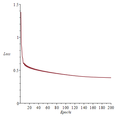
To test the trained network, we let the network’s prediction of a given professor rank be the argmax of the list of probabilities. We may now evaluate the accuracy on the training set and find that the ANN predicts professor rank correctly 12 out of 14 times! The list of predictions by the network is [4, 4, 4, 4, 2, 4, 3, 4, 3, 3, 4, 3, 1, 3], and the correct rankings are [4, 4, 4, 4, 2, 4, 4, 4, 3, 3, 4, 3, 1, 2].

It is interesting to see how our model performs with using fewer descriptive features. It seems that the number of publications, the number of citations, and the h-index are particularly important criteria, so we use these to train the ANN. Using the same hyper-parameters, the neural net trains well after 200 epochs. The loss curve is similar, yet we find that the ANN predicts the ranking correctly only 9 out of 14 times. The list of predictions is [3, 2, 3, 1, 3, 3, 4, 3, 3, 4, 4, 3, 4, 1] in comparison to the true rankings [3, 3, 3, 1, 2, 3, 4, 4, 4, 4, 4, 3, 4, 2]. It is instructive to plot the data to see how it is clustered. Below is a plot of the three-dimensional data where each points color represents the ranking of the professor: magenta corresponds to assistant professor, blue to associate professor, green to professor, and orange to distinguished professor.

Figure 6: The three-dimensional data where each points color corresponds to the ranking of the professor.

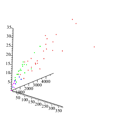
One can see that the data is not linearly separable, and in fact does not seem to be separable by any simple non-linear model. Future investigation could include finding a small number of parameters which allow for a linear separation of the data or seeing how well a non-linear model predicts professor rankings.

4.2 Exploration on Math Faculty Data with ANN

To use the entire data set, we attempt to predict AMS status, as this is a feature that is common across all departments and not subjective to internal departmental policy. Hence, we can use all the data of publication, citation and $h$-index information to predict whether a professor is an AMS fellow.

Since there are already numerous literatures on how to tune an ANN model and how to find the “best” hyperparameters, we merely give an example of code here. Following is an example of the algorithm. We use python’s keras package to explore the prediction.

Figure 7: Keras Package for ANN

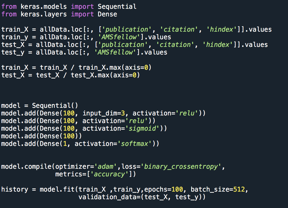
By preprocessing the input data, adding regularization, trying different architecture and activation functions, doing a grid search for hyperparameters and choosing suitable metrics to evaluate the model, it would be very promising to have a great precision in the prediction. The tuning and refining process is left to interested readers.

5 Unsupervised Clustering For Predictive Analysis

The method used in this section is an unsupervised clustering algorithm developed by the 2015 UCLA Applied Math REU Hyperspectral Imagery research team [4],[5]. It was chosen because it was designed specifically to sort large sets of data into a relatively small number of sorted groups, with no prior information or training data needed. The following terminology will be borrowed from the hyperspectral lexicon: each sorted group is called a cluster, and the average vector of a cluster is its centroid.

In the context of hyperspectral imagery, the NLTV algorithm is notable because there are very few robust unsupervised algorithms. Here, it is the lack of necessity of training data which makes it an interesting clustering method to apply: while data can be collected from universities across the country, there is no guaranteed standard of departmental promotions, which means each university ought to be treated separately, and as such that does not provide much training data for a neural network.

5.1 The Algorithm

The core of the sorting algorithm comes from the minimization of an energy functional

$$E(u)=\parallel\bigtriangledown u\parallel_{L1}+\lambda\langle u,f\rangle,$$ (5.1)

where $u:\Omega\rightarrow[0,1]^{n}$ is the labeling function on the data, $n$ is the number of clusters it is being sorted into, and $\Omega$ is the domain of the data, and f is a fidelity function. The inspiration comes from the imaging process technique of total variation introduced by Rudin et al in 1992 [9] for noise reduction, which corresponds to the minimization of the gradient of $u$. In highly noisy images or datasets where adjacent pixels do not matter, simply calculating the gradient directly does not give as pertinent information. Therefore, we turn to the theory of nonlocal operators introduced by [7],[8], Zhou and Schölkopf and adapted to image processing by Osher and Gilboa [10].

Let $\Omega$ be a region in $\mathbb{R}^{k}$, and $u:\Omega\to\mathbb{R}$ be a real function. Then the non-local derivative is defined as

$$\frac{\partial u}{\partial y}(x):=\frac{u(y)-u(x)}{d(x,y)},\hskip 10.0pt\text{for all }x,y\in\Omega$$ (5.2)

where $d$ is a positive distance between $x$ and $y$. With the following non-local weight defined as 5.3, we can re-write the non-local derivative as 5.4.

$$w(x,y)=d^{-2}(x,y)$$ (5.3)

$$\frac{\partial u}{\partial y}(x)=\sqrt{w(x,y)}(u(y)-u(x))$$ (5.4)

Then the non-local gradient $\bigtriangledown_{w}u$ for $u\in L^{2}(\Omega)$ as a function from $\Omega$ to $L^{2}(\Omega)$ is the collection of all partial derivatives

$$\bigtriangledown_{w}u(x)(y)=\frac{\partial u}{\partial y}(x)=\sqrt{w(x,y)}(u(y)-u(x)).$$ (5.5)

Note that here, “distance” can either refer to the standard Euclidean distance

$$d(x,y)=\sqrt{\sum_{i=1}^{k}(x_{i}-y_{i})^{2}},$$ (5.6)

the cosine distance

$$d(x,y)=1-\frac{x\cdot y}{||x||||y||},$$ (5.7)

or a linear combination of them.

The non-local energy functional we are trying to minimize takes the form of

$$E(u)=\parallel\bigtriangledown_{w}u\parallel_{L1}+\lambda\sum_{i=1}^{n}|u_{i}(x)g(x)-c_{i}|^{2},$$ (5.8)

where $\parallel\bigtriangledown_{w}u\parallel_{L1}$ is the $L^{1}$ norm on the space $L^{2}(\Omega,L^{2}(\Omega))$ defined as

$$\parallel v\parallel_{L^{1}}:=\int_{\Omega}\parallel v(x)\parallel_{L^{2}}dx=\int_{\Omega}\Big{|}\int_{\Omega}v(x)(y)^{2}dy\Big{|}^{\frac{1}{2}}dx$$ (5.9)

and the fidelity function is explicitly given by $\lambda\sum_{i=1}^{n}|u_{i}(x)g(x)-c_{i}|^{2}$, where $g(x)$ is the datapoint and $c_{i}$ is the $i$th cluster centroid. We explicitly discretize the labeling function and nonlocal operators, $u=(u_{1},u_{2},\ldots,u_{n})$ is a matrix of size $m\times n$, where $m$ is the number of datapoints and $n$ is the number of clusters. Each $u_{i}$ takes values between 0 and 1, $\sum_{i=1}^{n}u_{ki}=1$ for all $k\in{1,...,m}$. Then $(\bigtriangledown_{w}u_{l})_{i,j}=\sqrt{w_{i,j}}((u_{l})_{j}-(u_{l})_{i})$ is the nonlocal gradient of $u_{l}$; $(\text{div}_{w}v)_{i}=\sum_{j}\sqrt{w_{i,j}}v_{i,j}-\sqrt{w_{j,i}}v_{j,i}$ is the divergence of $v$ at $i$-th datapoint; and the discrete $L^{1}$ norm of $\bigtriangledown_{w}u_{l}$ are defined as:

$$\parallel\bigtriangledown_{w}u_{l}\parallel_{L^{1}}=\sum_{i}\left(\sum_{j}\left(\bigtriangledown_{w}u_{l}\right)_{i,j}^{2}\right)^{\frac{1}{2}}.$$ (5.10)

The functional 5.8 is convex, so a global minimum exists. However, calculating $\parallel\bigtriangledown u\parallel_{L^{1}}$ via gradient descent involves calculating div($\frac{\bigtriangledown u}{\mid\bigtriangledown u\mid}$), which is highly unstable because $\mid\bigtriangledown u\mid$ can be equal to zero. In 2011, Chambolle and Pock introduced a first-order primal dual algorithm, which they proved converged to a saddle point with a rate of $O(1/N)$ in finite dimensions for the complete class of convex problems [11]. This was used as an inspiration to craft a saddle point solution with respect to $u,$$\overline{u}$, and $p$. Full motivation and description can be found in [4], [5],[6]. The algorithm is as follows:

Primal-Dual Iterations
$\bullet$ Iterations $(n>0)$: Update $u^{n},p^{n},\bar{u}^{n}$ as follows:
$$\begin{cases}p^{n+1}=\text{proj}_{P}(p^{n}+\sigma\bigtriangledown_{w}\bar{u}^{n})\\ u^{n+1}=\arg\min_{u}\delta_{U}(u)+\frac{1}{2}\parallel(I+\tau F)^{\frac{1}{2}}u-(I+\tau F)^{-\frac{1}{2}}(u^{n}+\tau\text{div}_{w}p^{n+1})\parallel^{2}\\ \bar{u}^{n+1}=u^{n+1}+\theta(u^{n+1}-u^{n})\\ \end{cases}$$

where $F$ is the discretized fidelity function matrix with the inbuilt weight $\lambda$.

The overall sorting algorithm is then:

Nonlocal Total Variation Unsupervised Clustering
$\bullet$ Initiate parameters.
$\bullet$ Calculate weight matrix.
$\bullet$ Set $n$ random datapoints as the first iteration of centroids, set
…$u^{0}=\overline{u}^{0}=$ Matrix(m,n,$1/m$) and $p^{0}$ zeroed out.
while not converge do
……Inner Loop: Primal Dual Algorithm to find minimizing $u$.
……Outer Loop: Threshold $u$ into an assignment function, and use the new sorting of the data to update the centroids.
end

The NLTV algorithms was originally retooled for clustering of mathematical data by the authors in [1], which only used data from Rutgers University for sorting but included data on salaries. There are two main changes between the algorithm written for this paper, and the algorithm developed in 2015. Firstly, the calculation of the weight matrix is done directly between all datapoints in this project; the original hyperspectral algorithm used a “patch” distance to filter for noise, and employed an approximate nearest neighbor search to save computational time. In the original algorithm, a smart simplex clustering method instead of directly thresholding was developed for the hyperspectral with inspiration from [12]. The final thresholding process was not used in the analysis of the data as it makes the outerloop of the algorithm far more computationally expensive, for no increase in convergence time in a dataset as clean as this one.

There are a number of parameters involved in the algorithm, but the two most vital ones are $\lambda$, which determines the weight given to the minimization of the fidelity function vs the gradient of $u$, and the choice of Euclidean vs Cosine distance for the creation of the weight matrix and fidelity distance calculations. The value for $\lambda$ ought to be comparatively large to prioritize tight sorting. Euclidean vs Cosine vs a linear combination is something that should be tailored to the dataset, as some of the fields (ie h-index or AMS Fellow: 0/1) have a smaller range of values, and some of the fields (ie number of citations or year of PhD) have a much larger range of values, so that field does not dominate.

5.2 Results

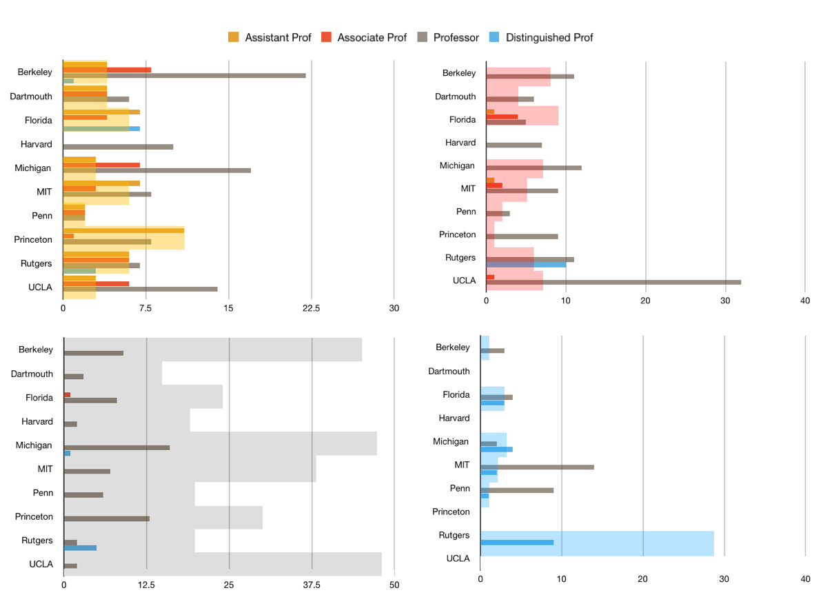
The individual results for the average three or four centroids of ten universities are listed in the charts below. ‘Rank’ indicates 1 for Assistant Professor, 2 for Associate Professor, 3 for Professor, and 4 for Distinguished Professor, which ‘AMS’ denotes 1 for AMS Fellow, and 0 if not. Figure 8 gives a secondary direct visual of the “accuracy” of each cluster by denoting the actual ranks of each professor sorted into the associated centroid. Some universities did not have Distinguished Professors, and hence the data was sorted into three clusters instead of four. Harvard only had Professors, and so was sorted into three clusters. Parameters ’cosine’ indicates Euclidean weight $10^{-10}$, Cosine weight 1, $\lambda=1$, and ’mixed’ indicates Euclidean weight 1, Cosine weight $10^{2}$, $\lambda=10^{4}$.

The general pattern of the results is as follows: the NLTV clustering algorithm is usually able to pick out the extremes correctly (i.e. placing all of Rank 1 or Rank 4 in the same cluster); however, the extremely large variance in the Professor / Rank 3 Category means that oftentimes multiple Professor clusters would form instead of the desired ranking.

Figure 8: Sorted Clusters Vs Ground Truth

Berkeley, Parameters: Mixed.

	Quantity	Rank	Publications	Citations	H-Index	AMS	Year of PhD
Centroid 1	35	2.571	36.686	445.400	11.029	.229	1999.143
Centroid 2	11	3	76.455	1471.818	19.909	.455	1986.636
Centroid 3	9	3	119.667	3636.889	30.778	.556	1980.667
Centroid 4	3	3	187.667	9024	38.667	1	1977.333

Dartmouth, Parameters: Cosine.

	Quantity	Rank	Publications	Citations	H-Index	AMS	Year of PhD
Centroid 1	14	2.143	20.857	106.286	5.500	0	1997.929
Centroid 2	6	3	46.167	528.167	11.333	0	1991.667
Centroid 3	3	3	92.333	1211	18	.333	1977.666

Florida, Parameters: Cosine.

	Quantity	Rank	Publications	Citations	H-Index	AMS	Year of PhD
Centroid 1	18	2	21.056	64.111	4.444	0	2001.778
Centroid 2	10	2.400	43.200	292.200	9.400	0	1991.700
Centroid 3	9	2.889	80.222	527.333	12.222	.111	1983.556
Centroid 4	7	3.429	98.857	1357.571	16.857	.143	1978.714

Harvard, Parameters: Cosine.

	Quantity	Rank	Publications	Citations	H-Index	AMS	Year of PhD
Centroid 1	10	3	56.700	1066.900	16.900	.300	1990.600
Centroid 2	7	3	106.429	3070.571	30.286	.571	1977.286
Centroid 3	2	3	313	11618	46.500	.500	1974.500

Michigan, Parameters: Cosine.

	Quantity	Rank	Publications	Citations	H-Index	AMS	Year of PhD
Centroid 1	27	2.516	23.704	162.444	6.593	0.111	1998.111
Centroid 2	12	3	87.917	1313.167	18.500	.500	1989.917
Centroid 3	17	3.059	59.588	744.824	13.706	.412	1990.412
Centroid 4	6	3.667	109.333	4212	27.667	.833	1970

MIT, Parameters: Cosine.

	Quantity	Rank	Publications	Citations	H-Index	AMS	Year of PhD
Centroid 1	18	2.056	20.167	113.222	6.167	.222	2004.722
Centroid 2	12	2.667	36.250	503.500	12.583	.250	1999.250
Centroid 3	7	3	182.571	5692.857	35.714	.857	1972.571
Centroid 4	16	3.125	80.563	1840.938	22.250	.563	1993.063

Penn, Parameters: Mixed.

	Quantity	Rank	Publications	Citations	H-Index	AMS	Year of PhD
Centroid 1	6	2.000	21.000	87.333	5.333	.167	2006.167
Centroid 2	3	3	33.667	309.333	8.667	.333	1993
Centroid 3	6	3	75.333	1289.167	18.167	.500	1981.833
Centroid 4	10	3.100	67	664.300	14.100	.500	1982.900

Princeton, Parameters: Cosine.

	Quantity	Rank	Publications	Citations	H-Index	AMS	Year of PhD
Centroid 1	20	1.850	18.450	274.200	7.60	.250	2009.550
Centroid 2	9	3	69.889	1732.222	21.889	.667	1986.333
Centroid 3	13	3	160.769	5240.231	35.692	.615	1978.846

Rutgers, Parameters: Cosine.

	Quantity	Rank	Publications	Citations	H-Index	AMS	Year of PhD
Centroid 1	22	2.318	27.864	158.364	6.818	.273	2000.091
Centroid 2	21	3.476	68.190	757.905	14.238	.571	1985.762
Centroid 3	7	3.714	106.571	1713.714	21.143	.857	1985.143
Centroid 4	9	4	159.667	3247.556	27.222	1	1972.778

UCLA, Parameters: Cosine.

	Quantity	Rank	Publications	Citations	H-Index	AMS	Year of PhD
Centroid 1	23	2.478	24.783	166.130	6.565	0.127	2002.087
Centroid 2	33	2.970	70.455	1333.212	17.393	0.455	1989.848
Centroid 3	2	3	299.5	15861.5	58.5	1	1981

6 Summary

In this paper, the exploratory analysis of the math faculty data is conducted and multiple mathematical and statistical methods are used to predict the ranks and AMS fellow status of a math faculty member from other independent variables such as the number of publications and the number of citations. There is a strong demonstration of statistical correlation of the properties examined within the groups, and even with the simpler methods employed, there seems to be much promising potential for the development of an automatic promotion algorithm. For public universities in the United States, salary is listed online and is an additional parameter that may be valuable to predict. We encourage future researchers to make use of the data we have collected and/or additional data and experiment with more refined methods, and academic departments to consider developing and implementing algorithmic promotion methods.

 

Contact information of the authors:

{vc362, di110, yao, zeilberger, tz188} at math dot rutgers dot edu

References

- [1] Victoria Chayes, Tong Cheng, Terence Coelho, Quentin Dubroff, Dodam Ih, Joe Olsen, Jason Saied, Yukun Yao, Doron Zeilberger, Tianhao Zhang, A Mathematical Analysis Of Mathematical Salaries and More. Experimental Mathematics Class Project, Rutgers, 2019. https://sites.math.rutgers.edu/~yao/DAMF.html
- [2] Francois Chollet, Deep Learning with Python, Manning Publications, 2017
- [3] Aurelien Geron, Hands-On Machine Learning with Scikit-Learn & TensorFlow, O’Reilly Media, 2017
- [4] Wei Zhu, Victoria Chayes, Alexandre Tiard, Stephanie Sanchez, Devin Dahlberg, Da Kuang, Andrea Bertozzi, Stanley Osher, Dominique Zosso, Nonlocal total variation with primal dual algorithm and stable simplex clustering in unspervised hyperspectral imagery analysis. Technical report, CAM report 15-44, UCLA, 2015.
- [5] Wei Zhu, Victoria Chayes, Alexandre Tiard, Stephanie Sanchez, Devin Dahlberg, Andrea L Bertozzi, Stanley Osher, Dominique Zosso, Da Kuang, Unsupervised classification in hyperspectral imagery with nonlocal total variation and primal-dual hybrid gradient algorithm. IEEE Transactions on Geoscience and Remote Sensing, Vol 55 Issue 5 pg 2786-2798, 2017.
- [6] Wei Zhu, Nonlocal Variational Methods in Image and Data Processing. PhD thesis, UCLA, 2017.
- [7] D. Zhou and B. Schölkopf. “Regularization on discrete spaces”. Springer, Berlin, Germany, pp. 361-368.
- [8] D. Zhou and B. Schölkopf. “Discrete regularization”. MIT Press, Cambridge, MA, pp. 221-232.
- [9] L. I. Rudin, S. Osher, E. Fatemi. “Nonlinear total variation based noise removal algorithms.” Physica D. 60: 259–268, 1992.
- [10] Guy Gilboa, Stanley Osher. “Nonlocal Operators with Applications to Image Processing.” SIAM Multiscale Model. Simul. 7(3), 1005-1028, 2008
- [11] Antonin Chambolle and Thomas Pock. “A First-Order Primal-Dual Algorithm for Convex Problems with Applications to Imaging.” Springer, Journal of Mathematical Imaging and Vision. 40(1), 120-145, 2011.
- [12] Nicolas Gillis, Da Kuang and Haesun Park. “Hierarchical Clustering of Hyperspectral Images Using Rank-Two Nonnegative Matrix Factorization.” IEEE, Transactions on Geoscience and Remote Sensing. 53(4), 2066-2078, 2015.
- [13] Leslie Valiant. “Probably Approximately Correct.” Basic Books, 2013.
- [14] D. Kelleher, Brian Mac Namee, Aoife D’Arcy. “Fundamentals of Machine Learning for Predictive Data Analytics.” The MIT Press, 2015.