Magnetic Field Geometry and Composition Variation in Slow Solar Winds: The Case of Sulfur

Abstract

We present an examination of the First Ionization Potential (FIP) fractionation scenario invoking the ponderomotive force in the chromosphere, and its implications for the source(s) of slow speed solar winds by using observations from The Advanced Composition Explorer (ACE). Following a recent conjecture that the abundance enhancements of intermediate FIP elements, S, P, and C, in slow solar winds can be explained by the release of plasma fractionated on open fields, though from regions of stronger magnetic field than usually associated with fast solar wind source regions, we identify a period in 2008 containing four solar rotation cycles that show repeated pattern of sulfur abundance enhancement corresponding to a decrease in solar wind speed. We identify the source regions of these slow winds in global magnetic field models and find that they lie at the boundaries between a coronal hole and its adjacent active region, with origins in both closed and open initial field configurations. Based on magnetic field extrapolations, we model the fractionation and compare our results with element abundances measured by ACE to estimate the solar wind contributions from open and closed field, and to highlight potentially useful directions for further work.

1 Introduction

The First Ionization Potential (FIP) fractionation effect, the phenomenon where abundances of low FIP elements (FIP $<$ 10 eV) are observed to be higher in corona than in the photosphere compared to high FIP elements (FIP $>$ 10 eV), has been studied for over five decades (Laming, 2004; Meyer, 1985a, b; Pottasch, 1963; Schmelz et al., 2012). It is known that the fractionation pattern in the solar wind can be generally categorized by solar wind type, and therefore understanding the fractionation mechanism can help us study the properties of the source regions of various solar winds. The fast winds ($\gtrsim$ 600 km/s) are known to show a low degree of FIP fractionation (Bochsler, 2007; Feldman et al., 1998) and are associated with open field lines emanating from coronal holes. On the other hand, slow winds ($\lesssim$ 600 km/s) from quiet sun and active regions show a high degree of FIP fractionation (Feldman et al., 1998; Schmelz et al., 2012). Spectroscopic observations of open and closed field show similar variations in FIP fractionation, supporting the origin of fast winds in coronal holes, and suggesting that slow winds are associated with closed loop structures on the solar surface which are subsequently opened up by reconnection with neighboring open field lines, a process known as interchange reconnection, though slow winds coming directly from open field is not ruled out.

While there are several theoretical models that attempt to explain the FIP effect (1994AdSpR..14..139A; Arge & Mullan, 1998; Schwadron et al., 1999; von Steiger & Geiss, 1989), Laming (2004) first introduced a model invoking the ponderomotive force, which arises from the interaction between chromospheric plasma and Alfvén waves propagating through or reflecting from the chromosphere. This model can reproduce the observed fractionation pattern from both open and closed field configurations (Laming, 2015), and also provides insight into the Inverse FIP effect (Baker et al., 2019). Recently, more subtle variations in FIP fractionation have been noted. Reames (2018) pointed out that intermediate FIP elements such as S, P, and C show a higher degree of fractionation in energetic particles originating from co-rotating interaction regions (CIRs) than they do in particles collected during gradual solar energetic particle events (SEPs), and that similar abundance pattern variations are seen in the presumed source regions for these energetic particle samples; slow speed solar winds for the particles from CIRs (see e.g. Giammanco et al., 2007; Ko et al., 2013) and the closed loop solar corona for SEPs (e.g. Laming et al., 1995). Reames (2020, see Fig. 2 therein) uses these and other abundance anomalies to develop models of the provenance of various SEP populations.

Laming et al. (2019) investigate this further, and find for a closed loop supporting resonant Alfvén waves (where the wave travel time from one loop footpoint to the other is an integral number of half wave periods) insignificant fractionation of S, P and C, while for open field (where no Alfvén wave resonance exists) S, P and C can become fractionated if the magnetic field is sufficiently strong, much stronger than that usually associated with fast solar wind origins. Therefore these abundances might offer some discrimination between slow solar wind originating in open or closed field configurations.

In this study, we aim to test this hypothesis by examining the possible correspondence between the enhanced fractionation of intermediate FIP elements in slow solar winds and the magnetic field geometry of their source regions which may evolve through interchange reconnection. We do so by surveying the extensive record of solar wind speeds and composition from ACE mission and investigating magnetic features on the Sun associated with the abundance anomaly we identify in slow winds. We also obtain profiles of the magnetic field strength at these source regions, estimate the fractionation values of various elements using the model outlined in Laming et al. (2019) with the field profiles as inputs, and compare the results with the observed fractionation values. Section 2 introduces the finding from ACE data and the identified magnetic features on the Sun, Section 3 discusses the modeling results, Section 4 gives some discussion and Section 5 concludes.

2 Reduction of ACE data and the identification of slow solar wind source location

In this study, we use the Solar Wind Ion Composition Spectrometer (SWICS; Gloeckler et al., 1998) 1.1 data and The Solar Wind Electron, Proton, and Alpha Monitor (SWEPAM) data that are publicly available from ACE level 2 database . The SWICS data consists of elemental abundances, charge state compositions, and kinetic properties of all major solar-wind ions from H through Fe from launch to August 23, 2011, at time resolutions of 1 hour, 2 hour, and 1 day, depending on the observable. We took the solar wind speed from the 2-hour data of He²⁺ bulk velocity, the abundances of He, C, Ne, Mg, Si, Fe with respect to O from the 2-hour data, and the abundances of N and S with respect to O from the 1-day data. We averaged all 2-hour data over a day centered at the recorded time of 1-day data, while excluding the data points that do not have the quality flag of 0 (“good quality data”, see release note ) or are associated with the solar wind type of coronal mass ejection (as compared with streamer winds or coronal hole winds, a rough classification based on functions of O⁷⁺/O⁶⁺ charge state ratio versus proton speed, according to the data description ). We then calculated the fractionations and their error values for each element by dividing the measured abundances and their error values by their respective photospheric abundances with respect to oxygen; the photospheric abundances for O, S, C, N, Fe were taken from Caffau et al. (2011) and those for Ne, He, Mg, Si were taken from Asplund et al. (2009).

Following our aim described in the introduction, we plot the time profiles of these daily solar wind speeds and elemental fractionation values and visually survey the record for the expected fractionation pattern in slow solar winds. We control the search with three qualitative requirements. First, we restrict our search to the time frame near solar minimum so that the following identification of the source solar feature of slow winds is less complicated. Second, we focus on the fractionation enhancement of sulfur, since there are no phosphorus data and the variation in carbon fractionation values, as we find, is relatively small and therefore its comparison with wind speeds is more uncertain. Lastly, we only accept the sulfur enhancements in slow winds that appear within repeated wind speed patterns over a few months, so that the identified correspondence is more likely associated with the same solar features reappearing on the Sun.

Figure 1 shows our data from 2008 January 1 to 2008 April 22, around the minimum of Solar Cycle 23. Each elemental fractionation value is plotted on an equal scale of max/min = 4 (colors) on top of the solar wind speed (200 km/s to 900 km/s, black). It shows a repeated sulfur fractionation enhancement corresponding to a drop in the solar wind speed. The appearance seems to be a part of a repeated solar wind speed pattern that shows two distinct fast streams, one short-lived followed by another one that goes over more gradual decrease, separated by the drop. Although the sulfur enhancement corresponding to the solar wind speed drop is present before and after this period too, the level of increase with respect to the low-level fractionation during surrounding times is quite distinct during this period. There are several other interesting features to note during this period. Low-FIP elements, Mg, Fe, and Si, all show enhanced fractionation with the sulfur enhancements. Based on observed abundance differences between coronal holes and closed magnetic loops, it had been long suspected (possibly naively) that the low-FIP elements fractionate more in winds originating in closed field structures, so their enhancements would suggest the repeated appearance of such structures on the solar surface. However S does not fractionate in this way in closed loops (Laming et al., 1995, 2019), and a high S/O abundance ratio might point to a solar wind origin in open field, a point we explore in more detail below.

Neon during this period shows a very distinct fractionation variation; the lowest fractionation value corresponding with the first fast wind, relatively sharp increase corresponding to the following slow wind, then steady values over mild decrease in the solar wind speed, followed by an uptick to the highest value at the second minimum of the wind speed cycle. Shearer et al. (2014) studied the solar wind neon abundance and its dependence on wind speed and evolution with the solar cycle using the same data as this study but in a statistical manner over the entire mission period. They find that the neon abundance values can be categorized by three solar wind types: fast wind from coronal holes which has the lowest neon/oxygen abundance ratio of Ne/O$\sim 0.097\pm 0.014$, slow wind from active regions which prevail during solar maximum with slightly higher abundance ratio of Ne/O$\sim 0.116\pm 0.017$, and slow wind from quiet sun (helmet streamers) which prevail during solar minimum with the highest abundance ratio of Ne/O $\sim 0.170\pm 0.025$ (Shearer et al., 2014).

In this work, the abundance ratio values for each phase we identify in this period corresponds with the results of Shearer et al. (2014): $\sim 0.074$ for the first fast wind, $\sim 0.126$ for the first slow wind, then $\sim 0.163$ for the second slow wind at the end of cycle. This Ne/O abundance ratio enhancement in the second slow wind coincides with a depletion in the He/O abundance ratio at DoY 32, 58 and 85 (marked with grey vertical dashed lines in Figure 1), a circumstance identified with gravitational settling in a coronal loop prior to release into the solar wind (Laming et al., 2019). Otherwise, the helium variation shows noticeable enhancements corresponding to sulfur enhancements during this time period (for the first, the third, and the last red vertical lines in Figure 1, most pronounced at the third one on DOY 66), which we return to in Section 4.

Figure 2 shows the spacecraft mapping data of the solar wind plasma at 1 AU ((a), available from http://www.predsci.com/%20mhdweb/spacecraft_mapping.php) and the corresponding synoptic map from 195 Å channel of the Extreme ultraviolet Imaging Telescope (EIT) (Delaboudinière et al., 1995) on board The Solar and Heliospheric Observatory (SOHO) (Domingo et al., 1995) for the first Carrington rotation cycle (CR2065) during this time period. For (a), the users are to locate the yellow circle corresponding to the target date and follow the green line emanating from it to identify the source location of the observed solar wind back on the Sun. If one identifies the sources of the winds detected on the dates over which the contained sulfur level rises and decays in CR2065 (from January 4 to January 11), it is apparent that the majority points to the equatorial coronal hole at the Carrington longitude$\sim$250 degrees with negative polarization, which is adjacent to an active region (AR10980). We confirmed that this pair of the negative equatorial coronal hole and the adjacent active region consistently appears at every sulfur peaks during this period (the AR 10980 decays over three rotations and the new AR 10987 appears at the same location in the fourth rotation, see Figure 3 (a)). Together with the low-FIP (Mg, Fe, Si) observation, it seems that the repeated sulfur enhancement in the first slow wind is possibly related to this coronal hole-active region pair structure.

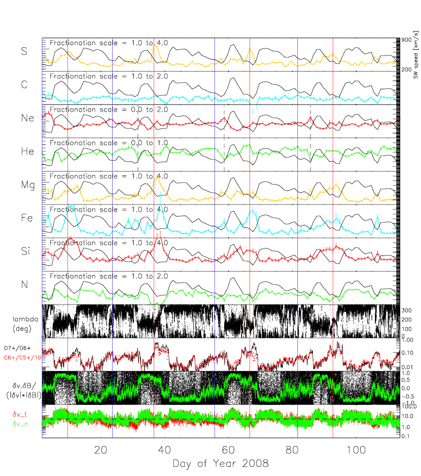
Figure 1: Top 8 panels: The daily solar wind speed (black) vs. fractionation values of various elements (colors) from 2008 January 1 to 2008 April 22. Repeated sulfur enhancement within a certain wind speed pattern, as well as interesting correspondences among various elements (see Section 2 for detail) can be seen. Bottom 4 panels: the orientation of IMF fields ($\sim 135$ degrees and $\sim 315$ degrees correspond to the inward and outward direction with respect to the nominal Parker spiral, respectively, 64s average), O⁺⁷/O⁺⁶ (black) and C⁺⁶/C${}^{+5}/10$ (red) charge state ratios (2-hour average), the quantity $(\delta v\cdot\delta B)/|\delta v||\delta B|$, which is a proxy of Alfvénicity (black for 64s average and green for their 1-hour average), and the velocity fluctuations in normal (green) and tangential (red) direction (64s average). The red and blue vertical lines mark the two kinds of slow wind that repeatedly appear during this period, one with sulfur enhancement and the other without sulfur enhancement, respectively.

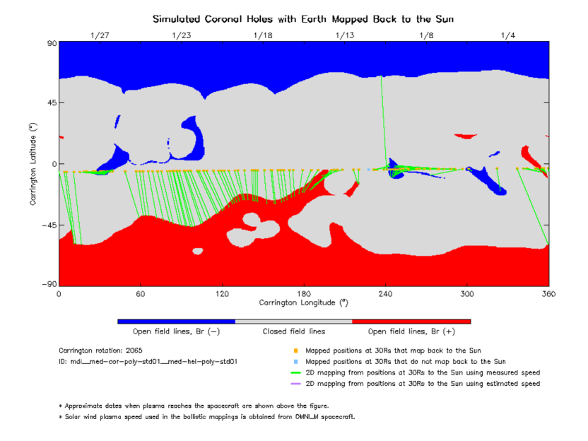
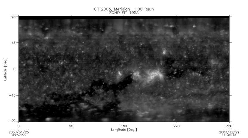
Figure 2: (a) Spacecraft mapping of the solar wind plasma at 1 AU, available from http://www.predsci.com/%20mhdweb/spacecraft_mapping.php for the first Carrington rotation cycle (2065). The users are to locate the yellow circle corresponding to the target date and follow the green line emanating from it to identify the source location of the observed solar wind back on the Sun. The first sulfur-enhanced slow winds were observed over January 4 to January 11, which suggests their source locations to be the negative coronal hole located at $\sim 250$ degrees, followed by the adjacent AR 10980. (b) The corresponding synoptic map from 195 Å channel of the EIT on board SOHO.

We additionally show in Figure 1 some of the data from SWEPAM during the same period in the bottom four panels. The first, lambda, is the 64s-average interplanetary (IP) magnetic field longitude in RTN coordinates, which indicates the magnetic field direction with respect to the nominal Parker spiral (inward and outward for $\sim 135$ degrees and $\sim 315$ degrees, respectively). The second is the hourly-averaged O${}^{+7}/$O⁺⁶ (black) and C${}^{+6}/$C${}^{+5}/10$ (red) charge state ratios. The third is the quantity $(\delta v\cdot\delta B)/|\delta v||\delta B|$, which is the normalized quantity that measures the degree of correlation between the IP velocity and magnetic fluctuation. This can be used as a proxy of Alfvénicity (Roberts et al., 1987; Ko et al., 2018), which measures how much of the fluctuations in the solar wind stream consist of pure Alfvén waves. Values of +1 or -1 mean pure Alfvén waves traveling in the opposite or the same direction as the mean field direction, respectively. The last is the velocity fluctuation in radial (r) and tangential (t) dimension. Ko et al. (2018) found that many dynamic parameters including the ones plotted in Figure 1 show distinctive changes in tandem during the interval defined by the low level of velocity fluctuations ($\delta v<5$ km/s, which is marked by the black dashed horizontal line in the bottom panel), which roughly coincides with interval between two fast wind streams. They found that, during this interval, Alfvénicity becomes closer to 0, the charge state ratio increases, and the IMF lambda reverses/does not change for the streams associated with a heliospheric current sheet (HCS)/pseudostreamer (PS) crossing where the two adjacent wind streams are from magnetic sectors of opposite/same polarity. They argued that this is due to the nature of the slow wind being more like the “boundary layer” from which it is generated as the certain spatial structure between two streams passes across the solar surface. We see in Figure 1 that there are two kinds of slow wind in every cycle in terms of the above-mentioned characteristics found by Ko et al. (2018), and one of them is associated with sulfur enhancement (marked by red vertical lines) and the other one is not (marked representatively by blue vertical lines based on the Alfvénicity value). The former is clearly associated with IMF lambda reversal from inward to outward in two streams, which corresponds with two coronal holes of opposite sign located over Carrington longitude of $\sim$200–250 degrees in Figure 2 (a), adjacent to the active region. On the other hand, the latter is associated with no sign change of IMF direction, and its outward direction corresponds to the large positive coronal hole shown in Carrington longitude of $\sim$0–180 degrees in Figure 2 (a), with no active region nearby. We therefore believe that our repeated sulfur enhancement is most likely related to the spatial structure of coronal hole-active region pair on solar surface.

Next, we investigated the magnetic field geometry of the source region of the sulfur-enhanced slow winds. To do so, we used the 1-hour cadence spacecraft mapping data of the solar wind plasma at 1 AU shown in Figure 2 (a) and the Potential Field Source Surface (pfss, 6-hour cadence; Schrijver, & De Rosa, 2003) package available in SolarSoft (Freeland & Handy, 1998). First, we obtain from the spacecraft mapping data all possible footpoint locations of the solar wind plasma detected at 1 AU over several days (4–7 days) covering the sulfur peak day (marked with red vertical lines in Figure 1). The beginning and the end date of this date range is defined by the first local minima of sulfur fractionation values counting backward and forward from the peak day. Next, we estimate the time that plasma detected on the sulfur peak day left the sun by dividing the Sun-spacecraft distance on the sulfur peak day by the solar wind speed measured on the sulfur peak day (both available from the spacecraft mapping data). Then, we obtain the pfss model closest to this time, and extract all field lines originating closest to the identified possible footpoint locations. Figure 3 (a) shows the resulting field lines next to the corresponding EIT 195Å images. It is apparent that sulfur-enhanced slow winds all come from the structure containing open fields from coronal hole and closed fields that belong to the adjacent active region. We also show the results for the “regular” slow winds marked by the blue vertical lines in Figure 1. The date range over which the solar wind footpoint locations were extracted was 4 days for all three dates. Compared to the sulfur peak dates, the quiet time solar wind traces back to the open fields with no significant magnetic feature nearby. Figure 4 shows the average magnetic field strength profile of all identified open field lines shown in Figure 3 for each day. Note that, for March sulfur peak, the positive open field line seen in Figure 3 was not included in the averaging process because the suggested IMF direction in Figure 1 for this date was inward. It is apparent that the field strengths are higher for the source regions of sulfur-enhanced slow winds since these field lines all originate near active regions. In the next section, we will use this magnetic field profile as an input to the ponderomotive force model of the FIP fractionation and compare the resultant fractionation of various elements with the observation.

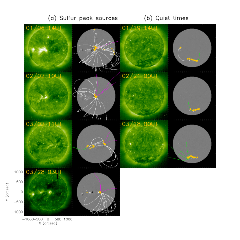
Figure 3: Field lines identified at the footpoint locations (orange crosses on the magnetograms) of the sulfur-enhanced slow wind ((a)) and of the regular slow wind ((b)), marked by the red and blue vertical lines in Figure 1, respectively, with corresponding EIT 195Å images. The white, magenta, and green field lines indicate the closed, negative open, and positive open field lines, respectively. The average magnetic field profiles of open field lines (only negative/magenta for (a)) were used for the modeling in Section 3.

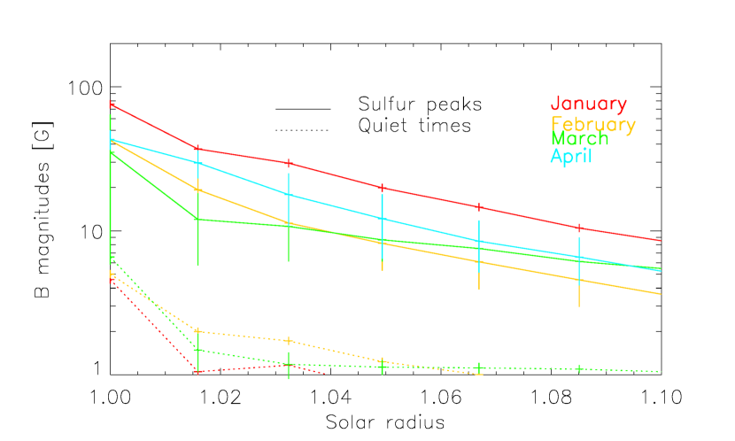
Figure 4: The average magnetic field profiles for the open field lines identified at the source regions of sulfur-enhanced solar winds and regular solar winds. The fields are stronger for the former because they all emanate from the region near active regions.

3 FIP modeling

In this section we attempt a quantitative interpretation of the abundance variations based on the model of fractionation by the ponderomotive force, guided by the magnetic field reconstructions. Alfvén waves causing the FIP fractionation can have either a coronal origin, presumably excited by nanoflares in closed loops (Dahlburg et al., 2016), or a photospheric origin deriving ultimately from fluctuations excited by convective motions. As in previous work (e.g. Laming, 2015) we construct model magnetic fields for open and closed field cases, and using the empirical chromospheric model of Avrett & Loeser (2008) integrate the Alfvén wave transport equations for a full non-Wentzel-Kramers-Brillouin (non-WKB) treatment of the wave propagation. For the time being we ignore terms giving wave damping or growth, and the wave origin only comes about as a matter of interpretation.

In closed loops, we take waves from nanoflares to be excited at the loop resonance or its harmonics. This is in general a higher frequency than the waves associated with convective motions originating lower down in the atmosphere, and the solution gives largest wave amplitude in the corona and ponderomotive force concentrated at the top of the chromosphere. In open loops, we take waves of period five minutes deriving from convection. Once the non-WKB wave solution is found by integrating the Alfvén wave transport equations, the instantaneous ponderomotive acceleration, $a$, acting on an ion is evaluated from the general form (see e.g. the appendix of Laming, 2017)

$$a={c^{2}\over 2}{\partial\over\partial z}\left(\delta E^{2}\over B^{2}\right)$$ (1)

where $\delta E$ is the wave (transverse) electric field, $B$ the ambient (longitudinal) magnetic field, $c$ the speed of light, and $z$ is a coordinate along the magnetic field.

Given the ponderomotive acceleration, element fractionation is calculated using input from the chromospheric model and the equation (Laming, 2017)

$$f_{k} = {\rho_{k}\left(z_{u}\right)\over\rho_{k}\left(z_{l}\right)}$$ (2)

$$= \exp\left\{\int_{z_{l}}^{z_{u}}{2\xi_{k}a\nu_{kn}/\left[\xi_{k}\nu_{kn}+\left(1-\xi_{k}\right)\nu_{ki}\right]\over 2k_{\rm B}T/m_{k}+v_{||,osc}^{2}+2u_{k}^{2}}dz\right\}.$$

This equation is derived from the momentum equations for ions and neutrals in a background of protons and neutral hydrogen. Here $\xi_{k}$ is the element ionization fraction, $\nu_{ki}$ and $\nu_{kn}$ are collision frequencies of ions and neutrals with the background gas (mainly hydrogen and protons, given by formulae in Laming, 2004), $k_{\rm B}T/m_{k}\left(=v_{z}^{2}\right)$ represents the square of the element thermal velocity along the $z$-direction, $u_{k}$ is the upward flow speed and $v_{||,osc}$ a longitudinal oscillatory speed, corresponding to upward and downward propagating sound waves. At the top of the chromosphere where background H is becoming ionized $\nu_{ki}>>\nu_{kn}$, and small departures of $\xi_{k}$ from unity can result in significant decreases in the fractionation. This feature is important in inhibiting the abundance enhancements of S, P, and C at the top of the chromosphere. Lower down where the H is neutral this inequality does not hold, and these elements can become fractionated.

The longitudinal oscillatory speed $v_{||,osc}$ is composed of sound waves deriving from convection (see Laming et al., 2019, for the most recent implementation) and sound waves excited by the Alfvén wave driver added in quadrature (see Laming, 2017). When this quadrature sum exceeds the local Alfvén speed, we assume that the resulting shock will produce sufficient turbulence and mixing to completely restrict further fractionation. For a parallel magneto-hydrodynamic shock, the first critical Alfvén Mach number is unity, and the shock must generate turbulence. Some observational evidence is given by Reardon et al. (2008).

In all prior work (Laming, 2015, 2017; Laming et al., 2019, e.g.) we have restricted the region of fractionation to be above the chromospheric equipartition layer where sound speed and Alfvén speed are equal. All fractionation is assumed to occur in low plasma-$\beta$ gas, where the plasma-$\beta=8\pi nk_{\rm B}T/B^{2}$ is the ratio of gas pressure to magnetic pressure. In the closed field geometry supporting resonant waves, this assumption makes no difference, because the ponderomotive acceleration is restricted to the top of the chromosphere by the non-WKB solution in any case. Here we give some further justification for this assumption in the open field situation.

Table 1: Model Fractionations for Slow Solar Wind Epochs 0, 2, 4 and 6

ratio	0		2		4		6
	open	closed	open	closed	open	closed	open	closed
Mg/O	2.92	2.62	3.36	2.87	2.84	2.66	2.89	2.51
Fe/O	2.47	2.53	2.87	2.83	2.76	2.75	2.46	2.45
Si/O	2.72	1.98	3.01	2.14	2.42	2.04	2.63	1.94
S/O	2.26	1.28	2.29	1.34	1.72	1.33	2.06	1.29
C/O	2.37	1.10	2.33	1.12	1.50	1.09	2.14	1.11
N/O	1.01	0.78	0.99	0.78	0.87	0.78	1.00	0.80
Ne/O	0.94	0.67	0.93	0.67	0.80	0.68	0.94	0.70
He/O	1.16	0.55	1.10	0.54	0.73	0.54	1.13	0.57

The dominant wave mode in the $\beta>1$ part of the atmosphere is acoustic, which can propagate at all angles to the magnetic field, and can effectively cascade to microscopic scales to cause mixing of the plasma, effectively quenching any fractionation. Higher up, where $\beta<1$, the magnetic field structures the plasma. Magnetosonic waves, which can propagate across the magnetic field, can escape laterally, leaving the Alfvén and acoustic waves, both of which are constrained to travel close to the magnetic field direction, in the FIP fractionation region. This constraint inhibits their cascade and the consequent plasma mixing, allowing the ponderomotive force to fractionate the plasma. The waves driven in the $\beta>1$ region are taken to be kink waves in magnetic flux concentrations (e.g. Cranmer & van Ballegooijen, 2005; Stangalini et al., 2013, 2015). Cranmer & van Ballegooijen (2005) describe how kink modes in the structured atmosphere at $\beta>1$ evolve to become transverse Alfvén waves as the magnetic field expands to fill up the volume when $\beta<1$. The mechanism of fractionation depends on the interaction of waves and ions (but not neutrals) through the refractive index of the plasma, and the effects this has on the refraction and reflection of waves. Waves are reflected (in the case of Alfvén waves) or refracted (for fast modes), and the resulting change in momentum of the wave is balanced by an impulse on the ions (see e.g. Ashkin, 1970, for an optical analog).

In addition to the fractionation coming from the ponderomotive force, a mass dependent fractionation comes from conservation of the first adiabatic invariant. This is evaluated from the magnetic field line expansion between close to the solar surface (see below) and 1.5 solar radii heliocentric distance. In Laming et al. (2019) we argued that at this point, the solar wind becomes collisionless, in the sense that the solar wind speed divided by the heliocentric radius becomes larger than the ion-proton collision frequency, $\nu_{ip}$, the reasoning being that at this point diffusion can no longer supply particles from the solar disk to counteract the abundance deficit caused by the extra acceleration, $a$. In Appendix A we give a slightly more rigorous treatment. The abundance modifications “freeze-in” when the ion thermal velocity $v_{t}<a/\nu_{ip}$, which leads to the same numerical conclusion.

Table 2: Model Fractionations for Slow Solar Wind Epochs 1, 3 and 5

ratio	1		3		5
	open	closed	open	closed	open	closed
Mg/O	1.73	1.61	2.14	1.93	1.70	1.55
Fe/O	1.68	1.69	1.97	1.97	1.61	1.56
Si/O	1.72	1.42	2.12	1.61	1.68	1.37
S/O	1.59	1.14	1.90	1.19	1.56	1.10
C/O	1.40	0.98	1.62	0.98	1.40	0.98
N/O	1.06	0.82	1.08	0.78	1.06	0.83
Ne/O	0.92	0.76	0.90	0.69	0.92	0.75
He/O	0.81	0.61	0.76	0.51	0.82	0.65

Table 3: Magnetic Field Parameters for Slow Solar Wind Epochs

epoch	0	1	2	3	4	5	6
$B\left(1.015R_{\sun}\right)$ (G)	37	1.05	19.3	2.0	12.0	1.5	29.7
$B\left(1.5R_{\sun}\right)(G)$	0.47	0.32	0.26	0.12	0.59	0.25	0.57
$\ln\left(B_{1.015}/B_{1.5}\right)$	4.4	1.2	4.3	2.8	3.0	1.8	3.9

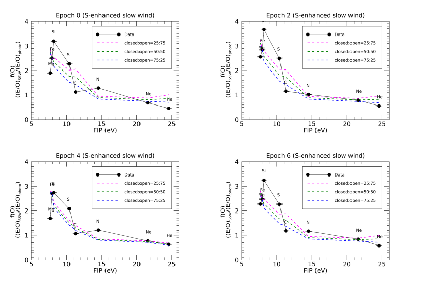
Figure 5: Fractionations with respect to O for Mg, Fe, Si, S, N, Ne, and He, plotted for epochs 0, 2, 4, 6 (black data points). Model fractionations give different proportions of plasma fractionated in open and closed field. Open field favors high S/O and high He/O.

The PFSS extrapolations use photospheric magnetograms as the lower boundary condition for the calculation of the coronal magnetic field. No account is taken here of magnetic field line expansion through the chromosphere as the plasma transitions from being gas pressure dominated ($\beta>1$) to being magnetic pressure dominated ($\beta<1$). We estimate the magnetic field in the ($\beta<1$) region of the chromosphere for the open field models from the values given by the extrapolations at 1.015 R_☉ (see Figure 4). Model fractionations for open and closed field cases are given Tables 1 and 2, for the “sulfur enhanced” slow wind (epochs 0, 2, 4, 6) and for epochs 1, 3, and 5 without strong sulfur fractionation, respectively, based on the magnetic field parameters given in Table 3. For the closed field calculations we assume 30 G and 2 G in Tables 1 and 2 respectively, though the fractionations are not sensitive to these values. Waves on closed loops are assumed to be shear Alfvén waves with amplitude in the corona around 30 - 100 km s^-1, depending on the coronal density assumed, while those on open fields are assumed to be torsional. The amplitude of the torsional wave varies depending on the magnetic field, with lower wave amplitudes ($\sim 25$ km s^-1 at 1.7 R_☉ where the integrations back to the Sun are started) required on the higher magnetic field epochs in Table 1 to provide the fractionation, rising to $\sim 200$ km s^-1 for epoch 4. This is because with higher magnetic field, fractionation occurs across a wider range of altitudes in the chromosphere, and corresponding smaller ponderomotive force is required. In Table 2, where the open magnetic field is much smaller, wave amplitudes at 1.7 R_☉ of 400 - 500 km s^-1 are required. For reference, the polar coronal hole model of Cranmer & van Ballegooijen (2005) gives (presumably r.m.s., derived from line broadening observations) wave amplitudes in this region of 100 - 200 km s^-1, and the fast solar wind models in Laming et al. (2019) require 300 km s^-1. The open field regions considered here have significantly lower magnetic fields than a typical polar coronal hole, and so might reasonably be expected to have higher wave amplitudes due to refraction effects.

For these open low magnetic field models, we have made an extra change to the chromospheric model. The hydrogen ionization balance given by Avrett & Loeser (2008), upon which our models are based, is elevated over that that would result from thermal equilibrium. This is presumably attributed to the effect of chromospheric shock waves, as in e.g. Carlsson & Stein (2002). A better match of theory to observations is found for the low open magnetic field regions by enforcing thermal equilibrium in the chromosphere, and using this assumption to calculate the explicit hydrogen ionization balance. The increased neutral fraction of hydrogen increases the degree of fractionation of other elements for a given ponderomotive force, and increases the relative fractionation of S/O and C/O. We argue that such “quiescent” chromosphere, with low magnetic fields and relatively faint in emission lines would not be picked up by the empirical procedures of Avrett & Loeser (2008), but nevertheless should be expected at the footpoints of open low magnetic field regions, where heating is taken to be proportional to magnetic field strength (e.g. Oran et al., 2017), and insignificant heat is conducted back downwards into the chromosphere from higher altitudes.

4 Discussion

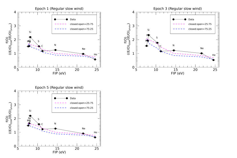
Figure 6: Fractionations with respect to O for Mg, Fe, Si, S, N, Ne, and He, plotted for epochs 1, 3, 5 (black data points). Model fractionations give different proportions of plasma fractionated in open and closed field.

The observed fractionations of various elements for each day are taken by averaging the values over the date ranges used for the solar wind footpoint identification in Section 2. In Figure 5 we compare data from the slow wind corresponding to the enhanced S/O abundance ratio with models, highlighted by the red lines in Figure 1, plotted as black symbols and compared to model fractionations calculated for various mixtures of plasma from closed and open magnetic field regions. The data are taken from approximately six day intervals, encompassing the peaks in the S/O, Mg/O, Fe/O and Si/O abundance ratios. The models for closed and open fields are designed to match the observed Fe/O ratio, with open field models reproducing the observed enhancement of S/O. Epochs 0, 2, 4 and 6 show qualitatively similar behavior to each other, with the S abundance relative to Fe being highest for the highest magnetic fields, (0, 6, 2, and 4 in descending order), both in data and in the open field models. The models also show a greater difference between open and closed field geometries for higher $B$. This is to be expected, since as explained above, the closed field only fractionates at the top of the chromosphere, while fractionation can occur from the $\beta=1$ layer upwards in open field, and the $\beta=1$ layer is pushed to lower altitudes when $B$ is higher. In general the open field models enhance S/O and C/O, while the closed field does not. The closed field depletes He/O while the open field does not, though Ne/O is well reproduced by both models. Roughly equal amounts of plasma fractionated in closed and open field appear to be present in this sample of slow speed solar wind.

The fractionation of Mg and Si with respect to Fe is not predicted by the models, and has been seen previously (Pilleri et al., 2015). Curiously, Heidrich-Meisner et al. (2018) re-analyze the same data using a different numerical procedure and find a different fractionation. For the range of O⁷⁺/O⁶⁺ charge state ratios (0.04 - 0.1) determined from Figure 1 (around the red vertical lines), Heidrich-Meisner et al. (2018) find Mg fractionated slightly more than Fe, and both are fractionated more than Si. This is the reverse of the trend found here and by Pilleri et al. (2015), and is in better agreement with our models. While the fractionation of Fe relative to Mg or Si is affected by the mass dependency introduced by the conservation of the first adiabatic invariant, the relative fractionations of Mg and Si depend much more on the ponderomotive force, with Mg being about 10% greater than Si in open field, and about 30% greater in closed loops.

Neither Pilleri et al. (2015) nor Heidrich-Meisner et al. (2018) considered the fractionation of S. Our models at least qualitatively capture this effect, with S considerably more fractionated in the open field than in the closed loop. Further support for this idea comes from a detailed inspection of Figure 1. The strong peaks in S/O appear before the corresponding peaks in Mg, Fe, and Si relative to O, by 0.5 -1 days, and both of these sets of features arrive at ACE about 0.5 days ahead of the low Alfvénicity turbulence. Bearing in mind that the minor ions generally flow faster than the bulk solar wind by a significant fraction of the Alfvén speed, $\alpha v_{A}$, and that the low Alfvénicity turbulence will be advected with the bulk solar wind, we interpret the strong peaks in Mg/O, Fe/O and Si/O as coming from a closed field region associated with the low-Alfvénicity turbulence, but arriving in advance at the spacecraft because of their faster speeds. In Appendix B we estimate this time difference to be $\sim\alpha v_{A}/v_{s}$ times the bulk solar wind travel time where $v_{s}$ is the bulk solar wind speed. This evaluates to a time of order 0.5 days, as observed. We further interpret the S/O peak to be more associated with the open field region and high Alfvénicity period just before the closed loop plasma, although at this point there will be considerable overlap between plasma originally in closed and originally in open fields.

C/O is also not observed to be enhanced along with S/O, as predicted by our models, and also based on expectations from prior work on SEPs (Reames, 2018), and solar wind measured by Ulysses (von Steiger et al., 2000) and ACE (Reisenfeld et al., 2007). These works typically give the C/O abundance ratio around 0.7, representing a fractionation of about 1.3 based on photospheric abundance of Caffau et al. (2011), though recent measurements of samples returned by the Genesis mission (Heber et al., 2013; Laming et al., 2017) give a ratio closer to 1, or a fractionation of $\sim 1.8$. For reasons that remain obscure, the C/O ratio measured herein on both open and closed fields stays close to that expected from closed field fractionation, with values 1 - 1.2, only marginally consistent with results quoted above. We have tried estimating the effect of molecular CO on the C and O fractionation. Taking partition functions from Rossi et al. (1985) and assuming local thermodynamic equilibrium we calculate the fraction of C and O atoms bound in molecules, and modify the fractionation calculations accordingly. In practice, outside of sunspots, this is a negligible effect. Similarly, the formation of H₂ to increase the neutral fraction of the background gas is not a significant factor.

It is worth noting the possible difference caused by different versions of ACE level-2 data; SWICS 1.1 data underwent a major new release around March 2015 using completely redesigned analysis method based on Shearer et al. (2014). We evaluated the possible effect that this change had in our study by recreating Figure 3 of Reisenfeld et al. (2007), which used the older version of ACE/SWICS data. We find that C/O fractionation is lower in the new data because O abundance is higher in the new data. We also find that Mg/Fe is less than 1 in the new data, which is in line with the discrepancy we mentioned earlier (Si/Fe is also less than 1 but higher than Mg/Fe). Despite these discrepancies, we find S/Fe to be consistent in both data sets: $\sim$0.78 in the new data and $\sim$0.74 in the old data. Therefore, the sulfur trend we find in this study seems to be unaffected by this data version change.

In Figure 6 we show similar plots for the epochs of non-S enhanced slow wind, which from Figure 4 is associated with much lower magnetic field strengths. The difference in fractionation between open and closed field is now smaller, as the $\beta=1$ layer moves upwards in the chromosphere, closer for open field to the region where fractionation is restricted to by the closed field. There is now better agreement in general between models and fractionations, (though fractionations are lower). The C/S ratio prefers the thermal equilibrium chromosphere discussed above, otherwise C is strongly overpredicted. This is the case for epochs 0, 2, 4, and 6, where the approximation of thermal equilibrium is less plausible here than for epochs 1-3-5, due to the higher magnetic field and increased heating (e.g. Oran et al., 2017). Among the low FIP ions, Si/O is consistently underpredicted, while the high FIP elements N/O, Ne/O and He/O are reproduced well. There are smaller differences here between open and closed field models due to the small magnetic field.

Several previous authors have studied high-Alfvénicity slow speed solar winds, either from the point of view of magnetic fields and waves/turbulence (e.g. Bale et al., 2019; Wang & Ko, 2019) together with imaging (Rouillard et al., 2020), or also including considerations of the wind composition (e.g. D’Amicis et al., 2019; Owens et al., 2020; Stansby et al., 2020). These last two make comparisons with the He/H abundance ratio, with Stansby et al. (2020) finding He/H observed by Helios (Porsche, 1977) in Alfvénic slow speed solar winds comparable to that in fast winds, and significantly higher than that found in non Alfvénic slow winds. This is in qualitative agreement with our results in Tables 1 and 2, though the precise quantitative agreement is less clear because ACE/SWICS and our models specify He/O. One feature we address that these other authors do not is the dependence of the He fractionation on the strength of the chromospheric magnetic field, which also seems to be borne out by our dataset.

Finally, for completeness, we mention solar wind periods shortly after epochs 3 and 5 where the Ne/O abundance ratio is enhanced, while the He/O abundance ratio is depleted. This is argued in Laming et al. (2019) to be a signature of pre-release gravitational settling, as found in ACE/SWICS observations by Weberg et al. (2012, 2015). Here, heavy elements are seen to be depleted with respect to H. The Ne/O and He/O behavior arises because He is most affected by gravitational settling, followed by O, and then Ne. Figure 6 in Weberg et al. (2012) indicates that they do indeed detect this region as a heavy ion dropout.

5 Conclusions

We have investigated a period of solar wind showing various repeatable element abundance modifications with a view to understanding the extent to which these can be explained by the ponderomotive force model of the ion-neutral separation (the FIP Effect), and testing some of the assumptions embedded in the model. Of the high FIP elements, S, P, and C have the lowest FIPs, and can be significantly ionized in the chromosphere. When the background gas is also significantly ionized, these elements do not fractionate due to back diffusion of the neutral fraction; only true low FIP elements fractionate. But when the background gas is neutral, minor elements ions and neutrals move through the background gas with equal ease, and S, P, and C can become fractionated. In our models, this can occur in open field regions where the magnetic field is sufficiently strong, due to the assumption that FIP fractionation only occurs above the plasma $\beta=1$ layer (discussed in Section 3). This arises because the $\beta=1$ layer is pushed to lower and lower altitudes by the increasing magnetic field, allowing more of the fractionation to occur in chromosphere plasma where H is neutral, consequently increasing S, P, and C. This effect is restricted to open fields, on the assumption that waves on closed loops are dominated by waves that are resonant with the loop, in the sense that the wave travel time from one footpoint to the other is an integral number of wave half-periods. In this case, the wave solution restricts fractionation to the upper chromosphere, no matter what the magnetic field strength is, and S, P, and C remain relatively unfractionated.

The thrust of this paper has been to study to what extent these ideas can be validated by direct solar wind observations. We have found solar wind intervals with large S/O abundance ratios that do indeed appear to be coming from open field regions with high magnetic field, and other solar wind periods associated with low magnetic field open region without significant S/O fractionation. While these conclusions largely depend on PFSS magnetic field extrapolations to identify solar wind source regions, they are also supported by observations of the Alfvénicity of the solar wind, and especially in the case of the large S/O solar wind, the time delay between the S/O peak and those for other low FIP elements, Fe/O, Mg/O, Si/O, etc, which probably come from closed field associated with low Alfvénicity solar wind. We suspect that the accuracy of our abundance modeling is mainly limited by the chromospheric model. Avrett & Loeser (2008) provide a static 1D “average” empirical chromosphere, which is certainly adequate for establishing the validity of the ponderomotive force as the agent behind the fractionation, and for understanding long term averages of solar wind abundances. More accurate fractionations will probably require incorporation of more details of chromospheric dynamics (e.g. Carlsson & Stein, 2002; Carlsson et al., 2019).

Appendix A Abundance Modification by Adiabatic Invariant Conservation

The transport equation for the solar wind distribution function $f$ is written

$${\partial f\over\partial t}+{\bf v}\cdot\nabla f+{{\bf F}\over m}\cdot\nabla_{\bf v}f={\rm scattering~{}terms}+{\rm particle~{}source~{}terms}$$ (A1)

with $f\propto\exp-\left({\bf v}-{\bf U}\right)^{2}/2v_{t}^{2}$ where ${\bf U}$ is the solar wind bulk velocity, ${\bf v}$ are the velocities of solar wind particles, and $v_{t}$ is the thermal speed. The force ${\bf F}$ includes all forces. In steady-state conditions, with ${\bf U}=U{\bf\hat{r}}$, ${\bf F}=F{\bf\hat{r}}$ and ${\bf B}=B{\bf\hat{r}}$ where ${\bf\hat{r}}$ is a unit vector in the radial direction, and separating out the action of the first adiabatic invariant from ${\bf F}$ we get,

$$v_{\|}{\partial f\over\partial r}+{v_{\|}v_{\perp}\over 2}{\nabla_{\|}B\over B}{\partial f\over\partial v_{\perp}}+\left[{F\over m}-{v_{\perp}^{2}\over 2}{\nabla_{\|}B\over B}\right]{\partial f\over\partial v_{\|}}=\nu_{ip}\left(v_{t}\over v\right)^{3}{\partial\over\partial\mu}\left[\left(1-\mu^{2}\right){\partial f\over\partial\mu}\right],$$ (A2)

where a term for minor ion collisions with protons has been included on the right hand side. With $\partial f/\partial v_{\|}=-\left(v_{\|}-U\right)/v_{t}^{2}$ and $\partial f/\partial v_{\perp}=-v_{\perp}/v_{t}^{2}$, and averaging over $v_{\|}$ and $v_{\perp}$,

$$U{\partial\left<f\right>\over\partial r}={U\over 2}{\nabla_{\|}B\over B}\left<f\right>=-{a\over v_{t}^{2}}\left<f\right>.$$ (A3)

where $a=v_{t}^{2}\nabla_{\|}B/2B$ is the acceleration resulting from the first adiabatic invariant conservation. In conditions where $\nabla_{\|}B/B<0$, the particle velocity increases and if nothing else happens, the abundance decreases to maintain constant particle flux. However diffusion induced by the negative concentration gradient will increase particle fluxes and abundances in the solar wind. The net flux will then be

$$J=-D{\partial\left<f\right>\over\partial r}={\rm min}\left(v_{t},-{v_{t}^{2}\over\nu_{ip}}{\nabla_{\|}B\over B}\right)\left<f\right>,$$ (A4)

where the diffusion coefficient $D=v_{t}^{2}/\nu_{ii}$, and the diffusive flux is limited to flow at less than the particle thermal speed. This implies a “freeze-in” of abundances when $\nu_{ip}<-v_{t}\nabla_{\|}B/B$. Compared with equation 1 in Laming et al. (2019), the term on the right hand side has changed from $v_{sw}/r$, where $v_{sw}$ is the solar wind velocity and $r$ the heliocentric radius, to $v_{t}/\left|l_{B}\right|$, where $l_{B}$ is the scale length of ${\bf B}$. Numerically, these amount to the same conclusion; abundances freeze-in at a density of $10^{5}-10^{6}$ cm^-3 at a heliocentric radius of $\sim 1.5R_{\sun}$.

Appendix B Parker Spiral Travel Times of Minor Ions and Background Plasma

Minor ions are known to flow at some fraction of the Alfvén speed, $\alpha v_{A}$, where $\alpha\sim 0.5$, faster than the bulk plasma, and consequently will arrive at in situ detectors before the plasma and entrained waves with which they might be associated. We consider a simple model where the solar wind speed, $v_{s}$, and the Alfvén speed, $v_{A}$ are taken as constant. The background plasma travel time is then

$$t_{plasma}=\int_{R_{\sun}}^{r}{dr\over v_{s}}={r-R_{\sun}\over v_{s}}$$ (B1)

while the minor ion travel time is

$$t_{ions}=\int_{R_{\sun}}^{r}{dr\over v_{s}+\alpha v_{A}\cos\left(\phi-\phi_{0}\right)}\simeq\int_{R_{\sun}}^{r}{dr\over v_{s}+\alpha v_{A}\cos\left({\omega\sin\theta\over v_{s}}\left(r-R_{\sun}\right)\right)}$$ (B2)

where the Parker spiral is given by the approximate equation ${\omega\sin\theta\over v_{s}}\left(r-R_{\sun}-R_{\sun}\ln{r\over R_{\sun}}\right)=\phi-\phi_{0}$ (e.g Priest, 2014), $\omega=2.8\times 10^{-6}$ rad s^-1 being the angular velocity of the solar rotation, $\theta$ the polar angle, with $\theta=\pi/2$ in the ecliptic plane,and $\phi$ and $\phi_{0}$ are the azimuthal angle made by the field line to the radial direction, and its initial value at $r=R_{\sun}$. An approximation to this equation has been substituted into the final form in equation B6. We write $z={\omega\sin\theta\over v_{s}}\left(r-R_{\sun}-R_{\sun}\right)$ and integrate to find

$$t_{ions}={2v_{s}\over\omega\sin\theta\sqrt{v_{s}^{2}-\alpha^{2}v_{A}^{2}}}\arctan\left\{\left(v_{s}-\alpha v_{A}\right)\tan{\omega\sin\theta\over 2v_{s}}\left(r-R_{\sun}\right)\over\sqrt{v_{s}^{2}-\alpha^{2}v_{A}^{2}}\right\}$$ (B3)

where $v_{s}>v_{A}$. If $v_{A}\rightarrow 0$, $t_{ions}\rightarrow\left(r-R_{\sun}\right)/v_{s}$ as expected. For $v_{A}>0$ but $<<v_{s}$, we find an approximate expression

$$t_{ions}\simeq{r-R_{\sun}\over v_{s}}\left(1-{\alpha v_{A}\over v_{s}}+\cdots\right)\simeq t_{plasma}-{r-R_{\sun}\over v_{s}}{\alpha v_{A}\over v_{s}}.$$ (B4)

Thus minor ions ($\alpha\sim 0.5$) will arrive before low Alfvénicity waves ($\alpha\sim 0$) which are essentially entrained in the plasma, but after waves with high Alfvénicity, travelling along the field at the Alfvén speed ($\alpha\sim 1$).

References

- Antiochos (1994) Antiochos, S. K. 1994, Advances in Space Research, 14, 139
- Arge & Mullan (1998) Arge, C. N., & Mullan, D. J. 1998, Sol. Phys., 182, 293
- Ashkin (1970) Ashkin, A. 1970, Phys. Rev. Lett., 24, 156
- Asplund et al. (2009) Asplund, M., Grevesse, N., Sauval, A. J., & Scott, P. 2009, ARA&A, 47, 481
- Avrett & Loeser (2008) , E. H., & Loeser, R. 2008, ApJS, 175, 229
- Baker et al. (2019) Baker, D., van Driel-Gesztelyi, L., Brooks, D. H., et al. 2019, ApJ, 875, 35
- Bale et al. (2019) Bale, S. D., Badman, S. T., Bonnell, J. W., et al. 2019, Nature, 576, 237
- Bochsler (2007) Bochsler, P. 2007, A&A Rev., 14, 1
- Caffau et al. (2011) Caffau, E., Ludwig, H.-G., Steffen, M., Freytag, B., & Bonifacio, P. 2011, Sol. Phys., 268, 255
- Carlsson & Stein (2002) Carlsson, M., & Stein, R. R. 2002, ApJ, 572, 626
- Carlsson et al. (2019) Carlsson, M., De Pontieu, B., & Hansteen, V. H. 2019, ARA&A, 57, 189
- Cranmer & van Ballegooijen (2005) Cranmer, S. R., & van Ballegooijen, A. A. 2005, ApJS, 156, 265
- Dahlburg et al. (2016) Dahlburg, R. B., Laming, J. M., Taylor, B. D., & Obenschain, K. 2016, ApJ, 831, 160
- D’Amicis et al. (2019) D’Amicis, R., Matteini, L., & Bruno, R. 2019, MNRAS, 483, 4665
- Delaboudinière et al. (1995) Delaboudinière, J.-P., Artzner, G. E., Brunaud, J., et al. 1995, Sol. Phys., 162, 291
- Domingo et al. (1995) Domingo, V., Fleck, B., & Poland, A. I. 1995, Sol. Phys., 162, 1
- Feldman et al. (1998) Feldman, U., Schühle, U., Widing, K. G., & Laming, J. M. 1998, ApJ, 505, 999
- Freeland & Handy (1998) Freeland, S. L., & Handy, B. N. 1998, Sol. Phys., 182, 497
- Giammanco et al. (2007) Giammanco, C., Wurz, P., Opitz, A., Ipavich, F. M., & Paquette, J. A. 2007, AJ, 134, 2451
- Gloeckler et al. (1998) Gloeckler, G., Cain, J., Ipavich, F. M., et al. 1998, Space Sci. Rev., 86, 497
- Heber et al. (2013) Heber, V. S., Burnett, D. S., Duprat, J., et al. 2013, LPSC, 44, 2540
- Heidrich-Meisner et al. (2018) Heidrich-Meisner, V., Berger, L., & Wimmer-Schweingruber, R. F. 2018, A&A, 619, A79
- Ko et al. (2018) Ko, Y.-K., Roberts, D. A., & Lepri, S. T. 2018, ApJ, 864, 139.
- Ko et al. (2013) Ko, Y.-K., Tylka, A. J., Ng, C. K., Wang, Y.-M., & Dietrich, W. F. 2013, ApJ, 776, 92
- Laming (2017) Laming, J. M. 2017, ApJ, 844, 153
- Laming et al. (2017) Laming, J. M., Heber, V. S., Burnett, D. S., et al. 2013, ApJ, 851, L12
- Laming (2015) Laming, J. M. 2015, Living Reviews in Solar Physics, 12, 2
- Laming (2004) Laming, J. M. 2004, ApJ, 614, 1063
- Laming et al. (1995) Laming, J. M., Drake, J. J., & Widing, K. G. 1995, ApJ, 443, 416
- Laming et al. (2019) Laming, J. M., Vourlidas, A., Korendyke, C., et al. 2019, ApJ, 879, 124
- Meyer (1985a) Meyer, J.-P. 1985, ApJS, 57, 151
- Meyer (1985b) Meyer, J.-P. 1985, ApJS, 57, 173
- Owens et al. (2020) Owens, M., Lockwood, M., Macneil, A., & Stansby, D. 2020, Sol. Phys., 295, 37
- Oran et al. (2017) Oran, R., Landi, E., van der Holst, B., Sokolov, I. V., & Gombosi, T. I. 2017, ApJ, 845, 98
- Pilleri et al. (2015) Pilleri, P., Reisenfeld, D. B., Zurbuchen, T. H., Lepri, S. T., Shearer, P., Gilbert, J. A., von Steiger, R., & Wiens, R. C. 2015, ApJ, 812, 1
- Porsche (1977) Porsche, H. 1977, J. Geophysics, 42, 551
- Pottasch (1963) Pottasch, S. R. 1963, ApJ, 137, 945
- Priest (2014) Priest, E. 2014, Magnetohydrodynamics of the Sun (Cambridge: Cambridge University Press)
- Reames (2018) Reames, D. V. 2018, SoPh, 293, 47
- Reames (2020) Reames, D. V. 2020, Space Sci. Rev., 216, 20
- Reardon et al. (2008) Reardon, K. P., Lepreti, F., Carbone, V., & Vecchio, A. 2015, ApJ, 683, L207
- Reisenfeld et al. (2007) Reisenfeld, D. B., Burnett, D. S., Becker, R. H. et al. 2007, Space Sci. Rev., 130, 79
- Roberts et al. (1987) Roberts, D. A., Klein, L. W., Goldstein, M. L., et al. 1987, Journal of Geophysical Research, 92, 11021.
- Rossi et al. (1985) Rossi, S. C. F., Maciel, W. J., & Benevides-Soares, P. 1985, A&A, 148, 943
- Rouillard et al. (2020) Rouillard, A. P., Kouloumvakos, A., Vourlidas, A., et al. 2020, ApJS, 246, 37
- Schmelz et al. (2012) Schmelz, J. T., Reames, D. V., von Steiger, R., & Basu, S. 2012, ApJ, 755, 33
- Schrijver, & De Rosa (2003) Schrijver, C. J., & De Rosa, M. L. 2003, Sol. Phys., 212, 165.
- Schwadron et al. (1999) Schwadron, N. A., Fisk, L. A., & Zurbuchen, T. H. 1999, ApJ, 521, 859
- Shearer et al. (2014) Shearer, P., von Steiger, R., Raines, J. M., et al. 2014, ApJ, 789, 60
- Stangalini et al. (2015) Stangalini, M., Giannattasio, F., & Jafarzadeh, S. 2015, A&A, 577, 17
- Stangalini et al. (2013) Stangalini, M., Solanki, S., Cameron, R., & Martinez Pillet, V. 2013, A&A, 554, 115
- Stansby et al. (2020) Stansby, D., Matteini, L., Horbury, T. S., Perrone, D., D’Amicis, R., & Berčič, L. 2020, MNRAS, 492, 39
- von Steiger & Geiss (1989) von Steiger, R., & Geiss, J. 1989, A&A, 225, 222
- von Steiger et al. (2000) von Steiger, R., Schwadron, N. A., Fisk, L. A., Geiss, J., Gloeckler, G., Hefti, S., Wilken, B., Wimmer-Schweingruber, R. F., & Zurbuchen, T. H. 2000, J. Geophys. Res., 105, 27,217
- Wang & Ko (2019) Wang, Y.-M., & Ko, Y.-K. 2019, ApJ, 880, 146
- Weberg et al. (2012) Weberg, M. J., Zurbuchen, T. H., & Lepri, S. T. 2012, ApJ, 760, 30
- Weberg et al. (2015) Weberg, M. J., Lepri, S. T. & Zurbuchen, T. H. 2015, ApJ, 801, 99