An Effective Field Theory for
Fractional Quantum Hall Systems near $\nu=5/2$

Abstract

We propose an effective field theory (EFT) of fractional quantum Hall systems near the filling fraction $\nu=5/2$ that flows to pertinent IR candidate phases, including non-abelian Pfaffian, anti-Pfaffian, and particle-hole Pfaffian states (Pf, APf, and PHPf). Our EFT has a 2+1$d$ O(2)_2,L Chern-Simons gauge theory coupled to four Majorana fermions by a discrete charge conjugation gauge field, with Gross-Neveu-Yukawa-Higgs terms. Including deformations via a Higgs condensate and fermion mass terms, we can map out a phase diagram with tunable parameters, reproducing the prediction of the recently-proposed percolation picture and its gapless topological quantum phase transitions. Our EFT captures known features of both gapless and gapped sectors of time-reversal-breaking domain walls between Pf and APf phases. Moreover, we find that Pf$\mid$APf domain walls have higher tension than domain walls in the PHPf phase. Then the former, if formed, may transition to the energetically-favored PHPf domain walls; this could, in turn, help further induce a bulk transition to PHPf.

1 Introduction

One of the first non-abelian topologically ordered candidate states was observed experimentally in 1987 [1]. It is the filling fraction $\nu=5/2$ fractional quantum Hall (fQH) state of an interacting electron gas in 2+1 spacetime dimensions (denoted as 2+1$d$). It has a fractional quantized Hall conductance $\sigma_{xy}=5/2$ in units of $e^{2}/h$ where $e$ is the electron charge and $h$ is the Planck constant. There have been many proposed candidate states to describe the underlying topological orders of this system: the major non-abelian candidates include Moore-Read’s Pfaffian state [2] (see also [3]), its particle-hole conjugate known as the anti-Pfaffian state [4, 5], and a particle-hole symmetric state known as the particle-hole Pfaffian state [6]. The particle-hole Pfaffian state [6] was originally proposed to be a particle-hole symmetric version of a composite fermion theory for the half-filled Landau level system [7]. Ref. [8, 9] made earlier attempts to propose candidate wavefunctions for the particle-hole Pfaffian state.

In 2017, a remarkable experimental measurement by Banerjee et al [10] suggested that the thermal Hall conductance of the $\nu=5/2$ fQH state is $\kappa_{xy}=5/2$ in units of $\pi^{2}k_{B}^{2}T/3h$, where $k_{B}$ is the Boltzmann constant and $T$ is the temperature.

In this work, we propose a unified bulk effective field theory (EFT) that give rise to various topological quantum field theories (TQFTs) and their edge modes pertinent to the $\nu=5/2$ fQH system. We map the EFT parameters to experimental quantities to produce a phase diagram in terms of the filling fraction (or the magnetic field) vs. the disorder strength. The phase diagram produced from our EFT turns out to be qualitatively similar to the previous theoretically proposed phase diagrams via the percolating phase transitions from the $2+1d$ disordered systems with random puddles and domain walls of Pfaffian and anti-Pfaffian states [13, 14, 15]. In the following, we first recall pertinent proposals from the literature.

1.1 Overview of theoretical proposals and questions

While both the theoretical proposals of Pfaffian state [2] and anti-Pfaffian state [4, 5] have a consistent fractional quantized Hall conductance $\sigma_{xy}=5/2$, their thermal Hall conductances, $\kappa_{xy}=7/2$ and $\kappa_{xy}=3/2$ respectively, seem to contradict with the result of [10]. By contrast, the particle-hole Pfaffian state proposed by Son in 2015 [6] predicts both $\sigma_{xy}=5/2$ and $\kappa_{xy}=5/2$, consistent with this recent experiment. On the other hand, vast numerical studies [18, 19, 20, 21, 22, 23, 24, 25, 26, 27] on the $\nu=5/2$ fQH system at low energy favor either the Pfaffian state or the anti-Pfaffian state. The dilemma between the experiment (favoring $\kappa_{xy}=5/2$) and the numerical data (favoring $\kappa_{xy}=7/2$ or $3/2$) raises an important issue: can the seemingly contradictory experimental and numerical results be reconciled?

Ref. [9] argued that the numerical simulations are simplified systems lacking both disorder (say, induced by impurities of experimental samples) and Landau-level mixing (LLM), which occur in real laboratory experiments. Ref. [9] further suggested that the particle-hole Pfaffian may be stabilized by disorder, i.e. LLM and impurities that break particle-hole symmetry. However, Ref. [9] did not provide analytic details on how disorder can help realize this possibility in practice.

Building on this suggestion, Ref. [13, 14, 15] investigated the possibility of particle-hole Pfaffian (PHPf) topological order emerging from disordered puddle systems of Pfaffian (Pf) and anti-Pfaffian (APf) states with percolating random domain walls.

We recall that:

1. Neither the Pf nor the APf state has particle-hole (PH) symmetry [28]. Both Pf and APf have their lower Landau levels fully occupied with spin-polarized electrons (which contribute $\sigma_{xy}=2$). However, in the absence of LLM, if we assume that spin-polarized electrons in the highest, half-filled Landau level (so there is another contribution of $\sigma_{xy}=1/2$ and $\nu=5/2$ in total) interact only through two-body interactions, then exact PH symmetry is present in the idealized Hamiltonian. With the PH symmetry at $\nu=5/2$, the two PH symmetry-breaking states, Pf and APf, are related by a PH transformation. Thus, they have the same energy and become two degenerate states at $\nu=5/2$. PH symmetry is broken away from $\nu=5/2$, so either Pf or APf is favored on each side of $\nu>5/2$ and $\nu<5/2$. At $\nu=5/2$, if PH symmetry is spontaneously broken, one of Pf and APf is realized.

2. With LLM, PH symmetry is only approximate, so the critical $\nu$ may be shifted to $\nu_{c}=5/2+\delta\nu$. Second-order perturbation theory from LLM modifies the Hamiltonian and induces PH-symmetry-breaking three-body interaction terms, so both Pf or APf can be candidate ground states near $\nu_{c}$. Whether Pf or APf is the candidate ground state for $\nu$ near $\nu_{c}$ partly depends on the sign of the three-body terms. For a small deviation away from $\nu_{c}$, we gain quasiparticles for $\nu>\nu_{c}$, and quasiholes for $\nu<\nu_{c}$. If the quasiparticles of APf have a lower energy than those of Pf for $\nu>\nu_{c}$, then in turn quasiholes of Pf have a lower energy than those of APf for $\nu<\nu_{c}$, due to their PH conjugate properties at $\nu_{c}$ (and vice versa). As long as $\nu$ is within the $\nu_{c}\simeq 5/2$ fractional quantized Hall plateau, we assume Pf is favored for $\nu<\nu_{c}$ (and hence APf is favored for $\nu>\nu_{c}$) for simplicity [4].

3. Under the presence of spatial disorder (e.g., quenched disorder arising from the presence of impurities, or spatial variations in the chemical potential) and spatial density fluctuations on the sample, many puddles of Pf or APf of radii $\ell_{0}$ would form, with puddle sizes bounded by $\ell_{B}<\ell_{0}<L$ where $\ell_{B}=\sqrt{\hbar c/eB}$ is the magnetic length under a magnetic field $B$, and $L$ is the sample size. The disorder-induced puddles [29] separate Pf and APf into patterns analogous to that of islands and seas in an archipelago (see the picture illustration in Fig. 1 and Fig. 3 in [15]). The boundaries of puddles then form $(1+1)d$ domain walls (between Pf and APf regions) hosting four gapless chiral real Majorana-Weyl fermions (with chiral central charge $c_{-}=4\times\frac{1}{2}=2$) and two copies of the so-called gappable non-chiral double-semion theory of compact complex bosons (with $c_{-}=0$, and $c_{L}=c_{R}=1$). It is proposed that the domain walls percolating in the bulk drive the bulk phase into the so-called percolating phase. The question about the nature of the percolating phase becomes the question of understanding whether the domain wall degrees of freedom are localized in the bulk or delocalized through the whole bulk-boundary system (see the picture illustration in Fig. 3 in [15]).

   Ref. [13, 14] modeled the $\nu=5/2$ system in terms of a checkerboard network (of alternating Pf and APf in each chequered pattern) known as a Chalker-Coddington network model [30] (previously used in modeling the integer quantum Hall plateau transition). Ref. [15] performed perturbative and non-perturbative analyses of the $(1+1)d$ edge theory on the domain wall between Pf and APf states at different disorder energy scales, with particular focus on the emergent symmetries

   1.2 Comparison of three related proposals on disordered percolating systems

   We compare the results of Ref. [13, 14, 15], which we also summarize pictorially in Fig. 1 and Fig. 2 below:

   

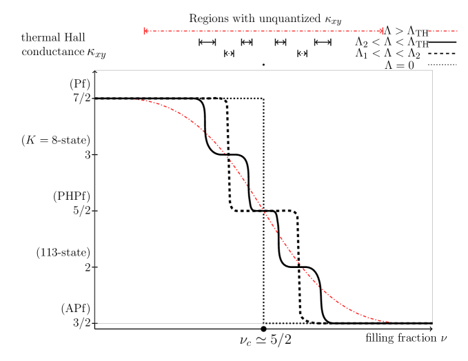
   Figure 1: Thermal Hall conductance $\kappa_{xy}$ vs filling fraction $\nu$ for the scenario proposed in Ref. [15]; see also Fig. 3 for a phase diagram. At different disorder energy scales $\Lambda$, we plot several curves of ($\nu$, $\kappa_{xy}$). At $\Lambda=0$, the $\kappa_{xy}$ (drawn as a dotted line) jumps at $\nu_{c}$ under a first order phase transition. From $0<\Lambda<\Lambda_{1}$, the jump can become smoother due to disorder. In the regime $\Lambda_{1}<\Lambda<\Lambda_{2}$, drawn as a dashed line, an intermediate $\kappa_{xy}=5/2$ plateau phase appears. Finally, when $\Lambda_{2}<\Lambda<\Lambda_{\rm{TH}}$, there are multiple plateau phases at $\kappa_{xy}=3,5/2$, and $2$. Notice that when $\Lambda>0$, all transitions between different quantized $\kappa_{xy}$ can have broadening, where the jumps at transitions become smoother slopes. On the top panel, we show different line intervals which represent the extent of broadening over ranges of $\nu$ demarcated on the horizontal axis, for the values stated of $\Lambda$ on the top right corner. When $\Lambda>\Lambda_{\rm{TH}}$, the slope is smooth enough to become a thermal metal so there is no quantized $\kappa_{xy}$ between 7/2 and 3/2. See Remark 3(3).

   

   

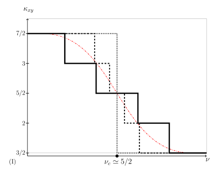
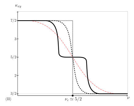
   Figure 2: Thermal Hall conductances: Scenario (I) from Ref. [13] (left) and scenario (II) from Ref. [14] (right). We use the same legend for drawing curves at different scales $\Lambda$ as in Figure 1. At $\Lambda=0$, $\kappa_{xy}$ (drawn as a dotted line) jumps at $\nu_{c}$ under a first order phase transition. For $\Lambda>0$, scenarios (I) and (II) differ. Scenario (I)’s $\kappa_{xy}$ has four jumps at the plateau for any $0<\Lambda<\Lambda_{\rm{TH}}$, and $\kappa_{xy}$ becomes smooth with non-quantized values for $\Lambda>\Lambda_{\rm{TH}}$.

   1. Ref. [13] proposed that a single first-order-like transition between Pf and APf occurs at $\nu_{c}$ and at zero disorder, due to an O(4) symmetry rotating four gapless chiral Majorana modes. The presence of these Majoranas induce a jump $\Delta\kappa_{xy}=\Delta c_{-}=2$. In the presence of any nonzero disorder, which weakly perturbs the first-order critical point, Ref. [13] proposed four consecutive continuous phase transitions (e.g., second-order transitions). Each transition causes $\kappa_{xy}$ to jump by 1/2, due to a single neutral chiral Majorana mode: from Pf ($\kappa_{xy}=7/2$) $\to$ $\kappa_{xy}=3$ $\to$ $\kappa_{xy}=5/2$ $\to$ $\kappa_{xy}=2$ $\to$ APf ($\kappa_{xy}=3/2$). Ref. [13] also expected the same universality class for disorder anisotropic models and uniform models. See the Fig. 1 phase diagram of [13]. We illustrate Ref. [13]’s thermal Hall prediction in Fig. 2’s (I).

   2. Ref. [14] suggested that for a finite range of $\nu\simeq\nu_{c}$, the Pf$\mid$APf domain walls percolate. If the charge neutral Majorana edge modes can diffuse freely in the network of domain walls in the bulk-boundary system, Ref. [14] proposed a thermal metal phase with an unquantized thermal Hall $\kappa_{xy}$ but a divergent $\kappa_{xx}$ (and, as usual, a quantized Hall conductance $\sigma_{xy}=5/2$, and $\sigma_{xx}=0$ at zero temperature). If the neutral Majorana modes are localized, Ref. [14] proposed a quantized $\sigma_{xy}=5/2$ phase with a quantized thermal Hall conductance $\kappa_{xy}=5/2$. Ref. [14] suggested that between the Pf and APf phases, there is a possible wide range of thermal metal behavior, even at low disorder. By tuning $\nu$, in the absence of disorder, there is a first-order-like transition between Pf $\to$ APf. At low disorder, there is a sequence of transitions from Pf $\to$ thermal metal $\to$ APf. At larger disorder, there is a sequence of transitions from Pf ($\kappa_{xy}=7/2$) $\to$ thermal metal $\to$ $\kappa_{xy}=5/2$ $\to$ thermal metal $\to$ APf ($\kappa_{xy}=3/2$). The intermediate thermal metal phase is a distinct key feature of [14]’s proposal. See the phase diagrams in Fig. 1 and Fig. 8 of [14]. We illustrate Ref. [14]’s thermal Hall prediction in Fig. 2’s (II).

   3. Ref. [15] performed perturbative and non-perturbative analyses on the $(1+1)d$ edge theory, and studied emergent symmetries on the domain wall between Pf and APf states at different disorder energy scales $\Lambda=\overline{v}/\ell_{0}$ (which is related to the inverse of the puddle size $\ell_{0}$ but proportional to the mean value of the edge state velocity $\overline{v}$). Then Ref. [15] proposed a more specific phase diagram of the $\nu=5/2$ disordered system, schematically shown in Fig. 3. An example of Ref. [15]’s thermal Hall prediction is illustrated in Fig. 1.

      

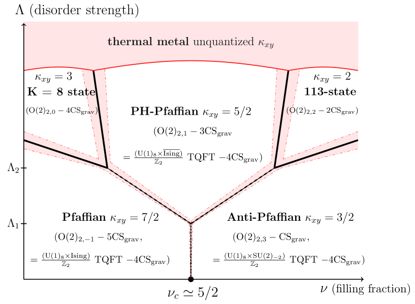
      Figure 3: A schematic phase diagram similar to Ref. [15]’s proposal. To see all these phases with varying $\kappa_{xy}$ requires that the $\nu_{c}\simeq 5/2$ plateau spans a sufficient range around $\nu_{c}$. Previous work [13, 14, 15] can obtain various quantized values of $\kappa_{xy}$ but cannot directly derive the bulk topological orders via the percolation transition argument. In this work, we propose a bulk effective field theory (EFT) not only consistent with [13, 14, 15] but can reproduce all the implicated bulk topological orders. At zero disorder, $\Lambda=0$, the transition at $\nu_{c}$ is first order. For $\Lambda>0$, there are different possibilities for transitions, depending on the microscopic details of samples. One scenario in [15] suggests that there are second order phase transitions (drawn in solid black lines) between topological orders for $\Lambda>0$. Another scenario in [15] suggests that there can be first order phase transitions between topological orders for $\Lambda>0$, but that disorder broadens these first order transitions to regions (light red shaded regions) with unquantized $\kappa_{xy}$. These broadened regions cannot merely be crossovers, because the topological orders and global symmetries are distinct on the two sides. The boundaries of these broadened regions (drawn as dash-dotted red curves) could also be second order phase transitions. At larger $\Lambda\gg\Lambda_{2}$, a percolation transition from topological order to a thermal metal, also with unquantized $\kappa_{xy}$, is known to be a second order phase transition (drawn as solid red curves). We propose a unified EFT in eqn. (2.1) in Sec. 2 and an upgraded version in Sec. 2.5 to describe all phases in the phase diagram.

      By the perturbative renormalization group (RG) analysis on disorder and scattering, Ref. [15] finds different emergent symmetries at different disorder energy scales. By a Berezinskii-Kosterlitz-Thouless (BKT)-type RG analysis, Ref. [15] finds for weak disorder

      $$\Lambda<\Lambda_{1}\simeq\overline{v}(\overline{v}^{2}/W_{v}^{*})^{-1/d_{v}},$$

      there is an emergent O(4) symmetry among the four gapless chiral Majorana modes. This describes a transition

      Pf ($$\kappa_{xy}=7/2 \to \kappa_{xy}=3/2$$) APf (). (1.1)

      (For $\Lambda=0$, this is a first order transition. For $0<\Lambda<\Lambda_{1}$, this can be a second order transition or a first order transition with weak disorder broadening the transition.) For

      $$\Lambda_{1}<\Lambda<\Lambda_{2}\simeq\hskip 1.0pt\mathrm{e}^{2}/\epsilon\ell_{B},$$

      where $\Lambda_{2}$ is set by the electron’s Coulomb interaction and $\epsilon$ is a dielectric constant, we have two transitions

      Pf ($$\kappa_{xy}=7/2 \to \kappa_{xy}=5/2 \to \kappa_{xy}=3/2$$) APf (). (1.2)

      (Again, the two intermediate steps can be first order transitions but with disorder broadening, or second order transitions.) For the disorder scale

      $$\Lambda_{2}<\Lambda<\Lambda_{\text{TH}},$$

      we have four transitions

      $$\text{ Pf ($\kappa_{xy}=7/2$) $\to$ $\kappa_{xy}=3$ $\to$ $\kappa_{xy}=5/2$ $\to$ $\kappa_{xy}=2$ $\to$ APf ($\kappa_{xy}=3/2$) },$$ (1.3)

      all of which can be (broadened) first order transitions, or second order.

      Finally, for $\Lambda>\Lambda_{\text{TH}}$, when the disorder is very strong, the $\kappa_{xy}$ becomes unquantized and we enter into the thermal metal (TH) regions (the light red area on the top of Fig. 3). The percolation transition to the thermal metal phase guarantees the divergence of the correlation length, which therefore guarantees that the transitions from all topological orders to the thermal metal (drawn as the red solid curves in Fig. 3) are second order phase transitions.

      Note that the aforementioned disorder-broadening regions have unquantized $\kappa_{xy}$ and hence can behave similarly to a thermal metal as an intermediate phase. However, to be a precise thermal metal, one needs to check that $\kappa_{xx}$ diverges at zero temperature.

      We expect the first-order disorder-broadening spreads to a region of size that is exponentially suppressed by $e^{-f(\Lambda_{1},\Lambda_{2})/\Lambda^{2}}$ with some functional form $f$ of $\Lambda_{1}$ and $\Lambda_{2}$ [14], which grows wider as the disorder increases (i.e. the light red area becomes wider in Fig. 3 along the phase boundaries) [29]. What might be the outcomes of this phase boundary broadening?

      • One possibility is that the broadening region becomes a new intermediate phase, such as a thermal metal, with unquantized $\kappa_{xy}$, while the split phase boundaries (the dotted red lines in Fig. 3 along the phase boundaries) become two new second order phase transitions.

      • Another possibility is that the percolation transition of the domain walls can be induced within the broadening region. Since at the percolation transition critical point, the domain wall size and correlation length diverge (at least for an infinite-sized system), this induces a new single second order transition within the broadening.

      Broadening regions cannot become crossovers between neighboring phases, because the bulk phases have different topological orders and/or global symmetries.

   In fact, Remark 3(3), following the scenario from Ref. [15], can be regarded as a general scenario that recovers both of the two scenarios from Remarks 3(1) and 3(2) in certain limits.

The key point for us is that Ref. [13, 14, 15] suggested that a $\kappa_{xy}=5/2$ plateau may be induced when Pf$\mid$APf domain walls percolate. However, Ref. [13, 14, 15] have not directly demonstrated that the resulting bulk order is indeed PHPf. Although PHPf has $\kappa_{xy}=5/2$, it remains an open question to show the bulk PHPf induces this $\kappa_{xy}=5/2$. In this work, we propose a unified effective field theory that can be viewed as a parent or mother quantum field theory at some higher energy scale, which at low energies can give rise to all the relevant IR TQFT phases listed in Fig. 3, including $K=8$, PHPf and 113-state, etc.

1.3 Outline

In the previous subsections, we have summarized several proposed phase diagrams in the literature for the $\nu=5/2$ fractional quantum Hall state. We will focus on reproducing the phase diagram of [15], illustrated in Fig. 3. Our $2+1d$ EFT will also be able, in special limits, to reproduce phase diagrams arising from the other proposals [13, 14], as will become clear in the subsequent sections. The EFT description also reproduces the $1+1d$ domain wall worldvolume theory predicted by [15], and it additionally fixes the type of phase transitions at the various phase boundaries (i.e. first order vs. second order). We also begin a preliminary study of the energetics of our EFT by performing computation of the domain wall tension, valid in a semiclassical limit, in the relevant phases. The tension of the walls differs in the Pf$\mid$APf and PHPf phases of the theory due to the presence of the chiral Majorana fermions in the former regime.

We conclude this introduction by summarizing the plan for the rest of this article.

In Sec. 2, we introduce our effective field theory, discuss its various IR phases, and describe in detail how it maps to the phase diagram in Fig. 3.

In Sec. 3, we describe the anyon spectra in the various IR phases of our EFT in terms of TQFTs and their quantum numbers, which will be matched to the many-body wavefunctions later (in Appendix F).

In Sec. 4, we analyze the domain wall theory and excitations in some detail. In particular, we study the gapless sectors and evaluate the tension of the walls.

In Sec. 5, we conclude, make final remarks, and point out several future directions.

Several appendices contain additional background and some technical details used in the body of the paper. In Appendix A, we review the relation between the gravitational Chern-Simons term and the thermal Hall response. In Appendix B, we describe abelian and non-abelian versions of $\mathbb{Z}_{2}$ gauge theory in $2+1d$. In Appendix C, we clarify some details about the fermion path integral and counterterms. In Appendix D, we discuss the procedure for gauging a one-form symmetry in a $2+1d$ TQFT. In Appendix E, we systematically introduce O(2)_2,L Chern-Simons theories, their Hall conductance, and other relevant physical properties. In Appendix F, we review the wavefunction descriptions of the IR TQFTs relevant for our study. In Appendix G, we provide some additional details regarding our one-loop computation of the domain wall tension.

2 Effective field theory near the critical filling fraction in $2+1d$

We now present our effective field theory (EFT).

2.1 Gauge sector, global symmetry, and ’t Hooft anomaly

The 2+1$d$ EFT consists of three sectors:

• $[{\mathrm{O}}(2)]$ gauge field with Chern-Simons (CS) term ${\mathrm{O}}(2)_{2,1}$ (in the notation of [37]).

• Two Dirac fermions $\Psi^{j}$ with flavor index $j\in\{1,2\}$ in the determinant sign representation of the $[{\mathrm{O}}(2)]$ gauge group. Namely, fermions are odd ($-1$) under the $\det([{\mathrm{O}}(2)])=\pm 1.$

• A real non-compact scalar $\phi\in\mathbb{R}$ field coupled to the Dirac fermions by a Yukawa term. The $\phi$ also has a Higgs potential.

To make the connection with fQH, the Chern-Simons gauge field is coupled to a background ${\mathrm{U}}(1)_{\text{EM}}$ gauge field. We begin by considering a particular mass term for the Dirac fermions and an even exponent scalar potential so that the EFT preserves particle-hole symmetry and captures the phase transition at the critical filling fraction $\nu_{c}$. More general extra deformations including

• Particle-hole symmetry-breaking potential (an odd exponent scalar potential) for $\phi$,

• Majorana mass terms for four Majorana fermions, where each complex Dirac $\Psi^{j}=\eta_{j1}+\hskip 1.0pt\mathrm{i}\hskip 1.0pt\eta_{j2}$ is written as two real Majorana $\eta_{j1}$ and $\eta_{j2}$, with $j\in\{1,2\}$,

will be considered in subsequent sections to produce the entire phase diagram of Fig. 3.

Explicitly, the theory is a 2+1$d$ gauged Gross-Neveu-Yukawa-Higgs theory coupled to a non-abelian Chern-Simons theory

$${\mathrm{O}}(2)_{2,1}\;\text{CS}+\sum_{j=1,2}\overline{\Psi}^{j}(\hskip 1.0pt\mathrm{i}\hskip 1.0pt{\ooalign{\hfil\hfil/\hfil\cr$D$}}_{\cal C}-g\phi)\Psi^{j}-m(\overline{\Psi}^{1}\Psi^{1}-\overline{\Psi}^{2}\Psi^{2})$$ (2.1)

$$\hskip 180.67499pt+\frac{1}{2}(\partial\phi)^{2}+{\mu^{2}\over 2}\phi^{2}-{\lambda\over 4}\phi^{4}-3\text{CS}_{\text{grav}}~{},$$

where ${\cal C}$ indicates that the fermions are odd under the charge conjugation ${\cal C}:\Psi_{j}\to-\Psi_{j}$ where $[\mathbb{Z}_{2}^{\cal C}]\subset[{\mathrm{O}}(2)]=[{\mathrm{SO}}(2)\rtimes\mathbb{Z}_{2}^{\cal C}]$ becomes part of the gauge group. Since the entire [O(2)] is gauged, the fermions couple to the O(2)_2,1 Chern-Simons gauge theory by this $\mathbb{Z}_{2}^{C}$ gauging (see Appendix E). Each of the complex Dirac fermions ($\Psi^{1}$ or $\Psi^{2}$), regarded as two real Majorana fermions respectively ($\Psi^{j}=\eta_{j1}+\hskip 1.0pt\mathrm{i}\hskip 1.0pt\eta_{j2}$), enjoys an O(2) global symmetry. There is a faithful $\frac{{\mathrm{O}}(2)\times{\mathrm{O}}(2)}{\mathbb{Z}_{2}}$ global symmetry rotating the two Dirac fermions independently that we will explain later below.

The theory can be obtained by starting from the decoupled semion theory ${\mathrm{U}}(1)_{2}={\mathrm{SO}}(2)_{2}$ CS and the Gross-Neveu-Yukawa theory and then gauging the diagonal $\mathbb{Z}_{2}$ symmetry that acts on ${\mathrm{SO}}(2)_{2}$ as the charge conjugation symmetry $[\mathbb{Z}_{2}^{{\cal C}}]$ and acts on the Gross-Neveu-Yukawa sector as the fermion parity $[\mathbb{Z}_{2}^{F}]$. This changes the gauge group from $[{\mathrm{SO}}(2)]$ to $[{\mathrm{O}}(2)]$. We add a fermionic counterterm for the $\mathbb{Z}_{2}$ gauge field, which gives the $\mathbb{Z}_{2}$ level in ${\mathrm{O}}(2)_{2,1}$, and makes the resulting theory still depend on the spin structure. The spin structure dependence only comes from this discrete gauged $\mathbb{Z}_{2}$ Chern-Simons level.

Despite the appearance of the Chern-Simons term, the theory in fact has a particle-hole PH symmetry, also called the time-reversal $CT$ symmetry (possibly with a ’t Hooft anomaly discussed later): $\Psi^{i}\rightarrow\epsilon^{ij}\gamma^{0}\Psi^{j}$ and $\phi\rightarrow-\phi$, so that $\phi$ transforms as a real-valued pseudoscalar. To see this, we express the theory in (2.1) as

$${{\mathrm{O}}(2)_{2,1}\;\text{CS}{+}\left((\mathbb{Z}_{2})_{0}\text{ coupled to Gross-Neveu-Yukawa}\right)\over\mathbb{Z}_{2}}~{},$$ (2.2)

where the quotient denotes gauging the $\mathbb{Z}_{2}$ one-form symmetry generated by the composite line given by the product of the ${\mathrm{O}}(2)$ Wilson line in the non-trivial one-dimensional representation and the $\mathbb{Z}_{2}$ electric line. We briefly review the notion of gauging one-form symmetries in Appendix D. The O(2)_2,1 Chern-Simons theory is time-reversal invariant by level/rank duality [38, 37]. Each of the two theories in the numerator has time-reversal zero-form symmetry and $\mathbb{Z}_{2}$ one-form symmetry, where the zero-form and one-form symmetries do not have a mixed anomaly (since gauging the one-form symmetry reduces the two theories to SO(2)₂ and the Gross-Neveu-Yukawa theory, respectively, both of which are time-reversal invariant). Therefore, the quotient theory is also time-reversal invariant.

As discussed in Appendix E.1, the theory can couple to a background U(1)_EM electromagnetic gauge field $A$ to have a fractional quantum Hall conductivity $\sigma_{xy}=5/2$ under the U(1)_EM electromagnetic charge’s transverse conductivity measurement. The U(1)_EM electromagnetic gauge field only couples to the Chern-Simons gauge field, and hence all the phases we discuss have the same Hall conductivity $\sigma_{xy}$.

We will consider phases with $\mu^{2}>0$, which implies that the real (pseudo-)scalar field $\phi$ condenses with a vacuum expectation value (vev):

$$\langle\phi\rangle=\pm v,\quad v\sim\mu/\sqrt{\lambda}>0~{}.$$ (2.3)

This spontaneously breaks the time-reversal $CT$ symmetry, and there can be two symmetry-breaking vacua exchanged by the (broken) symmetry transformation in the 2+1$d$ bulk. The spontaneously broken time-reversal symmetry $CT$ leads to a 1+1$d$ domain wall that interpolates between the two vacua. We will investigate the domain walls in Section 4.

Let us elaborate more on the global symmetries and gauge group in eqn. (2.1):

• Continuous global symmetries —

  If we turn off the mass deformation $m=0$, then the theory has an enlarged ${\mathrm{O}}(4)/\mathbb{Z}_{2}\equiv{\rm PO}(4)$ symmetry, where the four Majorana components from the two Dirac fermions transform in a vector representation of ${\mathrm{O}}(4)$. Let us explain why we mod out by a $\mathbb{Z}_{2}$ subgroup of the näive rotational O(4) global symmetry. The $\mathbb{Z}_{2}$ center of ${\mathrm{O}}(4)$ (in fact the same as $\mathbb{Z}_{2}^{F}\subset{\mathrm{SO}}(4)\subset{\mathrm{O}}(4)$, where $\mathbb{Z}_{2}^{F}$ sends $\Psi_{j}\to-\Psi_{j}$) is identified with the charge conjugation element $[\mathbb{Z}_{2}^{\cal{C}}]$ of the $[{\mathrm{O}}(2)]$ gauge group.

  If we turn on $m\neq 0$, there is a faithful $\frac{\left(\rm{O}(2)\times\rm{O}(2)\right)}{\mathbb{Z}_{2}}$ global symmetry in eqn. (2.1). We mod out by a $\mathbb{Z}_{2}$ subgroup of the näive $\rm{O}(2)\times\rm{O}(2)$ symmetry because the diagonal $\mathbb{Z}_{2}$ center of $\rm{O}(2)\times\rm{O}(2)$ (in fact the same as $\mathbb{Z}_{2}^{F}\subset\rm{SO}(2)\times\rm{SO}(2)\subset\rm{O}(2)\times\rm{O}(2)$, where $\mathbb{Z}_{2}^{F}$ sends $\Psi_{j}\to-\Psi_{j}$) is identified with the charge conjugation element of $[\mathbb{Z}_{2}^{\cal{C}}]$ of $[{\mathrm{O}}(2)]$ gauge group.

  By contrast, if we allow the four Majorana fermions to all have different masses, then there is no continuous global symmetry (because the fermion parity $\mathbb{Z}_{2}^{F}$ that flips the sign of the fermions is identified with a gauge rotation $[\mathbb{Z}_{2}^{\cal{C}}]$). The different mass deformations considered in the subsequent sections can be organized by the breaking pattern of $\rm{PO}(4)$. The continuous global symmetry $\text{PO}(4)$ that transforms the fermions has the standard mixed anomaly with the time-reversal $CT$ symmetry given by the 3+1d $\theta$ term for a $\text{PO}(4)$ background gauge field with $\theta=(\pi,\pi)$.

• Discrete global symmetries —

  1. $\mathbb{Z}_{2}^{f}$ fermion parity symmetry: This $\mathbb{Z}_{2}^{f}$ should not to be confused with the already gauged $[\mathbb{Z}_{2}^{F}]$ (acting by $\Psi_{j}\to-\Psi_{j}$ only in the Dirac fermion sectors). The $[\mathbb{Z}_{2}^{F}]$ and $[\mathbb{Z}_{2}^{\cal C}]$ charge conjugation are identified and both dynamically gauged due to ${\ooalign{\hfil\hfil/\hfil\cr$D$}}_{\cal C}$. (Neither $\Psi_{1}$ nor $\Psi_{2}$ are gauge-invariant local fermionic operators). In fact, the $\mathbb{Z}_{2}^{f}$ acts not on Gross-Neveu-Yukawa sector, but only on the O$(2)_{2,1}$ CS and $-3\text{CS}_{\text{grav}}$. Note that eqn. (2.1) is an intrinsically fermionic theory (defined on spin manifolds) because both O$(2)_{2,1}$ CS and $-3\text{CS}_{\text{grav}}$ are spin Chern-Simons actions whose UV completion, say on a lattice, requires some gauge-invariant local fermionic operators.

  2. $\mathbb{Z}_{4}^{CT}$-symmetry: This is the particle-hole (PH) symmetry, also known as the $CT$-symmetry. This is an anti-unitary symmetry. Its normal subgroup is the $\mathbb{Z}_{2}^{f}$ fermion parity, since $(CT)^{2}=(-1)^{f}$. As mentioned, $\Psi^{i}(t,x)\rightarrow\epsilon^{ij}\gamma^{0}\Psi^{j}(-t,x)$ and $\phi(t,x)\rightarrow-\phi(-t,x)$. We will further explain how the $CT$ acts on the CS theories in TQFT sectors in Sec. 3. The ’t Hooft anomaly of the $CT$ symmetry can be derived by adding a large time-reversal preserving mass $m$ to the fermions and studying the anomaly in the infrared PH-Pfaffian theory ${\mathrm{O}}(2)_{2,1}$ — our theory can have the $\upnu\in\mathbb{Z}_{16}$ anomaly of $CT$ symmetry with $\upnu=0$ for PH-Pfaffian₊ and $\upnu=8$ for PH-Pfaffian_- [39, 40, 41, 42, 43].

  3. $\mathbb{Z}_{4}$ one-form global symmetry [44] from the ${\mathrm{O}}(2)$ Chern-Simons theory: The $\mathbb{Z}_{2}$ subgroup is generated by the ${\mathrm{O}}(2)$ Wilson line in the determinant sign representation. The $\mathbb{Z}_{4}$ one-form symmetry has an ’t Hooft anomaly, characterized by the spin $\frac{1}{4}$ statistics of the generating line [45]. The ’t Hooft anomaly of the one-form symmetry is related to the fractional part of the Hall conductivity; see Appendix E.1 We will not focus on this global symmetry in this work.

  4. $\mathbb{Z}_{2}$ magnetic 0-form symmetry of the ${\mathrm{O}}(2)$ gauge field [37]. We will not discuss this symmetry in this work.

• Gauge sector —

  $${\mathrm{O}}(2)_{2,1}\;\text{CS}\cong\frac{{\mathrm{U}}(1)_{8}\times T_{L=1}}{\mathbb{Z}_{2}}\;\text{CS}\cong\frac{{\mathrm{U}}(1)_{8}\times(\overline{\text{Ising}}\times\text{(spin-Ising)})}{\mathbb{Z}_{2}}\;\text{CS}\\ \cong\frac{{\mathrm{U}}(1)_{8}\times({\frac{{\mathrm{SU}}(2)_{-2}\times{\mathrm{U}}(1)_{4}}{\mathbb{Z}_{2}}}\times({\mathrm{SO}}(3)_{1}\times{\mathrm{U}}(1)_{-1}))}{\mathbb{Z}_{2}}\;\text{CS}.$$ (2.4)

  The second line rewrites Ising and spin-Ising TQFTs as CS theories. For background information on this sector, see Sec. E around eqn. (E.2).

In the following subsections, we discuss several deformations of our theory (2.1):

1. In Sec. 2.3, we consider a $CT$-preserving mass deformation, but the $CT$-symmetry turns out to be spontaneously broken. The deformation explicitly breaks $\rm{PO}(4)={\mathrm{O}}(4)/\mathbb{Z}_{2}$ down to $({\mathrm{O}}(2)\times{\mathrm{O}}(2))/\mathbb{Z}_{2}$.

2. In Sec. 2.4, we add an odd polynomial potential in $\phi$ to our action, which explicitly breaks $CT$-symmetry, but preserves the $({\mathrm{O}}(2)\times{\mathrm{O}}(2))/\mathbb{Z}_{2}$ symmetry (or ${\mathrm{PO}}(4)$ if $m=0$).

3. In Sec. 2.5, we add additional Majorana mass terms that break the entire ${\mathrm{PO}}(4)$ symmetry, but preserve the $CT$-symmetry.

2.2 Physical arguments supporting the EFT

Here we provide some arguments and intuition to support our EFT from simple physical considerations, following the setup in Ref. [15], see Fig. 4.

2.2.1 From gapless or gapped Fermi surfaces to four gapless Majorana nodes

The first question to ask about our EFT eqn. (2.1) is: why do we introduce two Dirac fermions (or four Majorana fermions)? This can be understood from solving the Bogoliubov-de Gennes (BdG) equation [15], which allows us to analyze the gap function $\Delta({\vec{k},\vec{r}})$ around the domain wall between the Pf and APf region. We remind ourselves that the Pf and APf (and other related topological orders) can be obtained by the superconductivity (SC) pairing of composite fermions (CF) in the Halperin-Lee-Read (HLR) theory [7] or the superconductivity pairing of composite Dirac fermions (CDF) in Son’s theory:

$$\begin{array}[]{rcc}&\text{{CF (HLR)}}&\text{{CDF (Son)}}\\[5.69054pt] \text{Pf}:&p\text{-wave},&d\text{-wave}.\\[5.69054pt] \text{$K=8$ state}:&s\text{-wave},&p\text{-wave}.\\[5.69054pt] \text{PHPf}:&p^{*}\text{-wave},&s\text{-wave}.\\[5.69054pt] \text{$113$ state}:&d^{*}\text{-wave},&p^{*}\text{-wave}.\\[5.69054pt] \text{APf}:&f^{*}\text{-wave}&d^{*}\text{-wave}.\end{array}$$ (2.11)

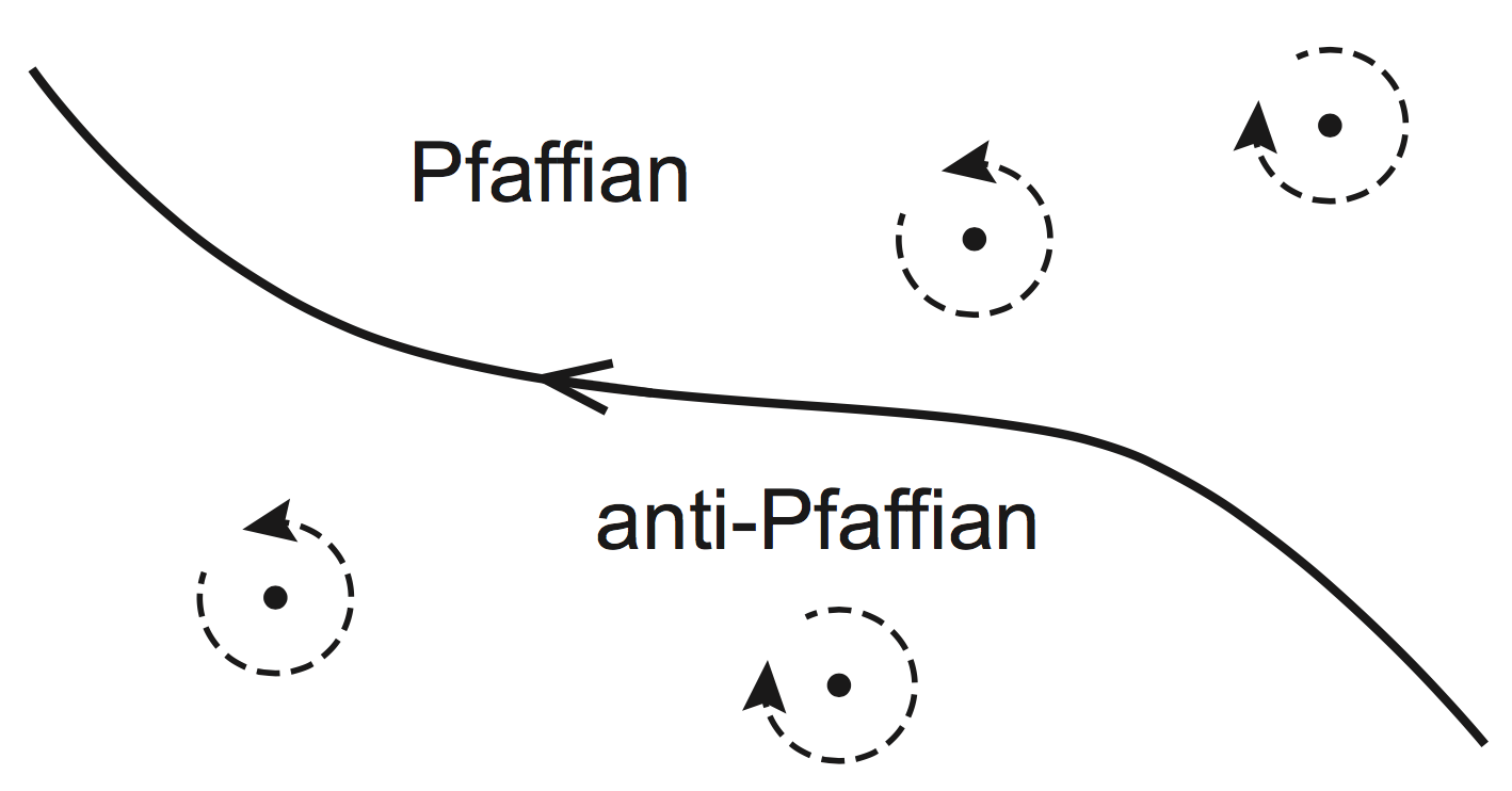
(a)     (b)

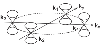
Figure 4: Follow the setup in Ref. [15]: (a) By solving the BdG equation in the mean-field, single-particle, semi-classical quantum mechanical manner [15], we can analyze the gap function $\Delta({\vec{k},\vec{r}})$ around the domain wall between the Pf and APf region. There are also $\pm\pi$ vortices shown in dashed circles. (b) Four Dirac nodes solved from the BdG equation on Pf$\mid$APf domain wall in a momentum $\vec{k}$-space. Due to BdG Nambu space double counting, we only have physical degrees of freedom of two Dirac nodes or four Majorana nodes. The four Majorana nodes are precisely the fermion nodes that we need in our EFT that we study in the real space.

The HLR and Son theories describe gapless theories with infinitely many gapless modes along a continuous Fermi surface (more precisely, a $1d$ Fermi circle for a $2+1d$ theory). However, we can gap the Fermi surface and go to a gapped theory by introducing the superconductivity pairing to CF or CDF as eqn. (2.11) above. Here we present the pairing gap function $\Delta(\vec{k})\propto(k_{x}+\hskip 1.0pt\mathrm{i}\hskip 1.0ptk_{y})^{L_{z}}$ to obtain the five topological orders in the phase diagram Fig. 3, where $s,p,d,f$-wave pairing has the $z$-directional angular momentum $L_{z}=0,1,2,3$ respectively, while the complex conjugate $p^{*},d^{*},f^{*}$-wave pairing has the opposite sign of the angular momentum.

We can find that in the CF (HLR’s) picture, the pairing function is $\Delta({\vec{k},\vec{r}})=\Delta_{\text{Pf}}(\mathbf{r})e^{\hskip 1.0pt\mathrm{i}\hskip 1.0pt\theta_{k}}-\Delta_{\text{APf}}(\mathbf{r})e^{-\hskip 1.0pt\mathrm{i}\hskip 1.0pt3\theta_{k}}\propto|\Delta|e^{-\hskip 1.0pt\mathrm{i}\hskip 1.0pt\theta_{k}}\sin({2\theta_{k}})$; while in the CDF (Son’s) picture, the pairing function is $\Delta({\vec{k},\vec{r}})=\Delta_{\text{Pf}}(\mathbf{r})e^{\hskip 1.0pt\mathrm{i}\hskip 1.0pt2\theta_{k}}-\Delta_{\text{APf}}(\mathbf{r})e^{-\hskip 1.0pt\mathrm{i}\hskip 1.0pt2\theta_{k}}\propto|\Delta|\sin({2\theta_{k}})$. In either case, the $\sin({2\theta_{k}})$ gives four gapless nodes around the otherwise fully gapped Fermi surface at $\theta_{k}=0,\pi/2,\pi,3\pi/2$, when we are spatially near the Pf$\mid$APf domain wall. Thus, Ref. [15] finds four Dirac nodes solved from the BdG equation on Pf$\mid$APf domain wall in a momentum $\vec{k}$-space. Due to BdG Nambu space double counting degrees of freedom at $\vec{k}$ and $-\vec{k}$, we only have physical degrees of freedom of two Dirac nodes or equivalently four Majorana nodes. The four Majorana nodes explain precisely the origin of the fermions that we need in our EFT eqn. (2.1) that we study in the real space. Furthermore, it will become clear in the later subsections how the additional gauge theory sectors and deformations can help to span the full phase diagram Fig. 4. This physical picture helps to motivate our EFT.

Our EFT, including the deformations, can describe both the gapped TQFT phases and gapless topological quantum phase transitions predicted in the phase diagram Fig. 3, similarly to the percolating phases and transitions in Ref. [15]. For condensed matter purposes, we remark that the $2+1d$ gapless phases in our Lorentz invariant EFT have four interacting Majorana fermions ($2+1d$ Majorana cones in a momentum $\vec{k}$-space, in the non-interacting band theory limit in Fig. 4 (b)) but without a Fermi surface — the Fermi surface is gapped and left with only isolated gapless nodes. In other words, we emphasize that the $2+1d$ gapless phase transitions in our EFT are similar to that of a semi-metallic phase transition with isolated gapless nodes, instead of a metallic phase transition with a gapless continuous Fermi surface.

2.2.2 More on energy and length scales, and emergent symmetries

Before we dive into the detailed phase diagrams of our EFT in the next subsections, we first summarize what we expect from the story in Ref. [15], about the energy and length scales (see also footnote 11), and emergent symmetries of the system.

We take the limit of no Landau-level mixing (LLM), so the energy gap between Landau levels from the cyclotron frequency $\omega_{c}=B/m\gg\Lambda_{2}=e^{2}/\epsilon\ell_{B}\sim\sqrt{B}$ is assumed to be much larger than the Coulomb energy scale, which we set to be $\Lambda_{2}$, the disorder energy scale in Fig. 3. The $\ell_{B}=\sqrt{\hbar c/eB}$ is the magnetic length scale. There is yet another length scale set by the domain wall width w, which is microscopically related to the phase-coherence length $\ell_{\varphi}$ of superconducting pairing fluctuations in the composite fermion picture of eqn. (2.11).

Ref. [15] analyzes the relation between energy/length scales and emergent symmetries of the $1+1d$ domain wall, showing that:

• The disorder energy $\Lambda\sim 1/\ell$ (the vertical axis of Fig. 3) is related to the domain length scale $\ell$ which controls the Pf and APf puddle sizes.

• The energy scale $\Lambda_{2}$ is defined by the inverse of magnetic length scale $\ell_{B}=\sqrt{\hbar c/eB}$. The $\Lambda_{2}$ is around the Fermi energy of the composite fermion.

• The energy scale $\Lambda_{1}$ is defined by the inverse of the correlation length $\ell_{\varphi}$ of superconducting phase pairing fluctuations in the composite fermion picture of Pf and APf, which is also related to the inverse of the domain wall width w.

• When the disorder energy scale $\Lambda<\Lambda_{1}$, we have weaker disorder and hence larger Pf and APf puddle sizes, so the domain length scale $\ell$ is large. For large $\ell$, the $1+1d$ four Majorana edge modes running on the domain wall can be mixed together via scattering along the domain wall, which induces an emergent O(4) symmetry and a uniform velocity.

• When the disorder energy $\Lambda$ scale sits at $\Lambda_{2}>\Lambda>\Lambda_{1}$, then $\Lambda$ is below the Coulomb energy $e^{2}/\epsilon\ell_{B}$ and the Fermi energy $\overline{v}k_{F}$ set by $\Lambda_{2}$. The $\Lambda$ is also below some factor of the magnitude of SC gap size $|\Delta|$. This implies that, from Fig. 4 (b), the two physical Dirac nodes solved from BdG, have internal symmetries ${\mathrm{O}}(2)\times{\mathrm{O}}(2)$, where each ${\mathrm{O}}(2)$ rotates the two Majorana nodes of a give Dirac node.

• When the disorder energy scale $\Lambda>\Lambda_{2}$, we have stronger disorder $\Lambda\sim 1/\ell$, hence smaller Pf and APf puddle sizes, so the domain length scale $\ell$ is smaller. For smaller $\ell$, it is difficult to mix the $1+1d$ four Majorana edge modes running on the domain wall, so we expect only the fermion parity symmetry when $\Lambda>\Lambda_{2}$. The ${\mathrm{O}}(2)\times{\mathrm{O}}(2)$ symmetry will be broken when $\Lambda>\Lambda_{2}$, because the disorder is strong enough to exceed the gap size $|\Delta|$ or even the Fermi energy $\overline{v}k_{F}$, so the Dirac nodes in Fig. 4 (b) fluctuate and their dispersion and energy spectra can overlap with each other. Because of this, we can no longer make sense of the two internal rotational symmetries.

To summarize all the length scales, we have

$$\text{ lattice cutoff $a_{\text{lattice}}$ $<$ magnetic length $\ell_{B}$ $<$ domain wall width w }\cr\text{ $\simeq$ phase-coherence length $\ell_{\varphi}$ $\lesssim$ \text{our EFT typical length scale} $\xi$ $<$ sample size $L$. }$$ (2.12)

The energy scales are given by the inverse of length scales:

$$a_{\text{lattice}}^{-1}>\Lambda_{2}=\ell_{B}^{-1}>\Lambda_{1}=\ell_{\varphi}^{-1}\simeq{\text{w}}^{-1}\gtrsim\xi^{-1}>L^{-1}.$$ (2.13)

2.3 Particle-hole (time-reversal $CT$)-preserving deformation

Let us turn on the deformation $m$ in eqn. (2.1).

${0\leq m<gv:}$

When $m$ increases from zero to $gv$, the theory has the following phases in the two vacua:

• At the vacuum $\langle\phi\rangle=-v$, $\Psi^{1}$ has mass $m-gv$, while $\Psi^{2}$ has mass $-m-gv$. For $m$ below $gv$, at low energies we can integrate out both negative mass Dirac fermions, and the theory becomes the gapped TQFT

  $$\text{Pfaffian}:\quad{\mathrm{O}}(2)_{2,-1}\;\text{CS}-5\text{CS}_{\text{grav}}~{}.$$ (2.14)

  The O(2)_2,L Chern-Simons gauge theory (see Appendix E) contains a ${\mathrm{U}}(1)_{8}$ Chern-Simons theory that contributes a net chiral central charge $c_{-}=c_{L}-c_{R}=1$, while the matter sectors do not contribute any net chiral central charge. The theory has Hall conductivity $\sigma_{xy}$ and thermal Hall conductivity $\kappa_{xy}$ matching those of the Pfaffian state:

  $$\sigma_{xy}=5/2,\quad\kappa_{xy}=1+5/2=7/2.$$

• At the vacuum $\langle\phi\rangle=+v$, $\Psi^{1}$ has mass $m+gv$, while $\Psi^{2}$ has mass $-m+gv$. For $m$ below $gv$, then at low energies we can integrate out the two positive mass Dirac fermions, and the theory becomes the gapped TQFT

  $$\text{anti-Pfaffian}:\quad{\mathrm{O}}(2)_{2,3}\;\text{CS}-\text{CS}_{\text{grav}}~{}.$$ (2.15)

  The theory has Hall conductivity $\sigma_{xy}$ and thermal Hall conductivity $\kappa_{xy}$

  $$\sigma_{xy}=5/2,\quad\kappa_{xy}=1+1/2=3/2.$$

  The TQFT becomes, under level/rank duality [38, 37], ${\mathrm{O}}(2)_{2,3}\leftrightarrow{\mathrm{O}}(2)_{-2,1}$ up to $4\text{CS}_{\text{grav}}$, and thus it is the time-reversal image of the Pfaffian theory.

The two different regimes capturing our time-reversal-symmetric deformations are depicted in Figure 5.

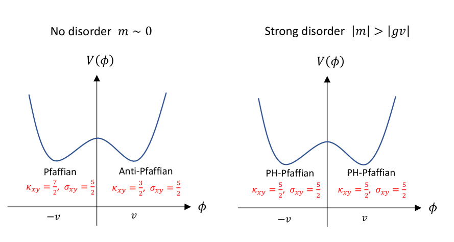
Figure 5: The theories comprising the vacua of the system (2.1) depend on the deformation $m$.

${m=gv:}$

When $m=gv=g|\langle\phi\rangle|$, one of the Dirac fermions becomes massless, and the theories are

$$\langle\phi\rangle=-v:\quad{\mathrm{O}}(2)_{2,0}\;\text{CS}+\Psi^{1}\text{ in }\mathbf{1}_{\text{odd}}-4\text{CS}_{\text{grav}}~{}.$$ (2.16)

$$\langle\phi\rangle=+v:\quad{\mathrm{O}}(2)_{2,2}\;\text{CS}+\Psi^{2}\text{ in }\mathbf{1}_{\text{odd}}-2\text{CS}_{\text{grav}}~{}.$$ (2.17)

${m>gv:}$

When $m>gv$, the two Dirac fermions acquire masses of opposite signs, and the two vacua become the same gapped TQFT

$$\text{PH-Pfaffian}:\quad{\mathrm{O}}(2)_{2,1}\;\text{CS}-3\text{CS}_{\text{grav}}~{}.$$ (2.18)

The theory has the Hall conductivity $\sigma_{xy}$ and thermal Hall conductivity $\kappa_{xy}$

$$\sigma_{xy}=5/2,\quad\kappa_{xy}=1+3/2=5/2.$$

With $m$ treated as a proxy for disorder strength (the precise relation is discussed in Section 2.6), the gapped phases in the above discussion are precisely those that appear in the scenario of [14, 15]: for small disorder strength, the microscopic theory is at a first order-like phase transition with coexisting Pfaffian and anti-Pfaffian phases, while increasing the disorder strength produces the PH-Pfaffian phase. From the above discussion, it is thus natural to identify the parameter $m$ (or its magnitude $|m|$) in the effective phenomenological theory with the disorder strength in the microscopic material.

We remark that the first-order phase transition with distinct gapped vacua persists for a range of the parameter $m\in[0,gv)$, which is consistent with the phase diagram proposed in [14, 15]. We may identify $\Lambda_{1}$ in [14, 15] with $gv$, with $v$ controlled by the scalar mass $\mu$ in the effective theory. When $gv$ is small, the phase diagram approaches that described in [13, 14].

2.4 Particle-hole (time-reversal $CT$)-breaking deformation

In this section, we investigate the effect of adding a time-reversal-breaking deformation that preserves the $\frac{{\mathrm{O}}(2)\times{\mathrm{O}}(2)}{\mathbb{Z}_{2}}$ symmetry ($\frac{{\mathrm{O}}(4)}{\mathbb{Z}_{2}}$ when $m=0$). In the experiment, this corresponds to applying an additional time-reversal-breaking magnetic field that changes the filling fraction $\nu$ slightly. In this discussion, we set the Yukawa coupling to $g=1$ for simplicity.

Since $\phi$ is a time-reversal-odd pseudoscalar field, we consider the simple time-reversal-breaking deformation given by an odd polynomial of $\phi$. The most relevant deformation will be $\delta V(\phi)\propto-m_{odd}\,\phi$. This modifies the scalar potential and lifts the degenerate vacua.

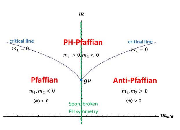
Figure 6: Phase diagram of the theory (2.1) deformed by the PH-symmetry breaking scalar potential $\delta V(\phi)=-m_{odd}\,\phi$. Phase boundaries are plotted analytically by Mathematica. Here the parameter $m$ is from the Dirac mass term in (2.1). The $m_{1}$ and $m_{2}$ are the induced masses in the IR for the ground states: $m_{1}=m+g\langle\phi\rangle$, $m_{2}=-m+g\langle\phi\rangle$. The blue lines are critical lines where one of the Dirac fermion becomes massless, joined by blue dots where both fermions are massless at a critical $m=gv=g|\langle\phi\rangle|$. The green line in the middle represents a first order phase transition with spontaneously broken time-reversal symmetry ($i.e.$, anti-unitary particle-hole symmetry) that gives rise to domain wall excitations that interpolate between the Pfaffian and anti-Pfaffian phases. The phase diagram is in qualitative agreement with the schematic phase diagram discussed in [14, 15] with the time-reversal breaking deformation $m_{odd}$ identified with the external magnetic field in the experiment and the time-reversal preserving deformation $|m|$ identified with the microscopic disorder strength. In experiment, it is so far undetermined whether Pfaffian or anti-Pfaffian is favored at $\nu<\nu_{c}\simeq 5/2$ (or $\nu>\nu_{c}\simeq 5/2$); we can easily flip our phase diagram by defining the sign of $m_{odd}$ to match the tuning parameter for the filling fraction $\nu$.

In the lowest-order approximation, we can take the effect to be such that the original vacua shift to the locations $\langle\phi\rangle=v+m_{odd}+{\cal O}(m_{odd}^{2})$ and $-v+m_{odd}+{\cal O}(m_{odd}^{2})$. Depending on the sign of $m_{odd}$, one of the above is the true vacuum: for $m_{odd}>0$ it is the former and for $m_{odd}<0$ it is the latter. In other words, the true vacuum has a vev:

$$\langle\phi\rangle=v\text{ sgn}(m_{odd})+m_{odd}+{\cal O}(m_{odd}^{2})=(v+|m_{odd}|)\text{ sgn}(m_{odd})+{\cal O}(m_{odd}^{2}).$$

The two Dirac fermions then have masses given by (with $g=1$)

$$m_{1}=m+\langle\phi\rangle=m+m_{odd}+v\text{ sgn}(m_{odd})+{\cal O}(m_{odd}^{2})~{},$$

$$m_{2}=-m+\langle\phi\rangle=-m+m_{odd}+v\text{ sgn}(m_{odd})+{\cal O}(m_{odd}^{2})~{}.$$ (2.19)

There are critical lines when any of the fermions become massless.

The phase diagram whose coordinates are our two parameters $(m,m_{odd})$ for a fixed $v$ is given in Figure 6. Given by the mass deformation formula (2.19), the left critical line in Figure 6 has $m_{2}\simeq 0$, while the right critical line in Figure 6 has $m_{1}\simeq 0$. It is in qualitative agreement with the schematic phase diagram discussed in [14, 15], and suggests that the corresponding Pf$|$PHPF and APf$|$PHPf phase boundaries are given by second-order phase transitions.

2.5 $K=8$ and $113$ states from $\frac{\mathrm{O}(2)\times\mathrm{O}(2)}{\mathbb{Z}_{2}}$-breaking masses

In our earlier discussion, we mainly focused on mass deformations preserving the $\frac{\mathrm{O}(2)\times\mathrm{O}(2)}{\mathbb{Z}_{2}}$ symmetry that transforms the two Dirac fermions. If we allow Majorana masses that break the $\frac{\mathrm{O}(2)\times\mathrm{O}(2)}{\mathbb{Z}_{2}}$ symmetry, the effective theory can also describe the $K=8$ state and the 113 state (the two states are related to one another by the particle-hole $CT$ symmetry). Denote the four Majorana fermions by $\eta_{ia}$ where $i=1,2$ labels the Dirac fermions and $a=1,2$ labels the Majorana components. Consider the Majorana mass deformation:

$$-M(m)\left(\eta_{11}^{2}-\eta_{12}^{2}-\eta_{21}^{2}+\eta_{22}^{2}\right),\quad M(m)=\epsilon(m-m^{*})\Theta(m-m^{*})~{},$$ (2.20)

where $\epsilon$ is a small number, $\Theta$ is the step function: $\Theta(x)=0$ for $x\leq 0$ and $\Theta(x)=1$ for $x>0$. Then the deformation is only nonzero when $m>m^{*}$, where we take $m^{*}>gv$. The deformation preserves the time-reversal $CT$ symmetry. The four Majorana fermions have masses

$$m_{11} =m+g\langle\phi\rangle+M(m),$$ (2.21)

$$m_{12} =m+g\langle\phi\rangle-M(m),$$ (2.22)

$$m_{21} =-m+g\langle\phi\rangle-M(m),$$ (2.23)

$$m_{22} =-m+g\langle\phi\rangle+M(m),$$ (2.24)

where the vev $\langle\phi\rangle=v\text{ sgn}(m_{odd})+m_{odd}+{\cal O}(m_{odd}^{2})$ depends on the CT symmetry-breaking deformation $m_{odd}$.

What becomes of the phase diagram under the deformation? For $m\leq m^{*}$ it is the same as before, while for $m>m^{*}$ there are new gapped phases:

• $m_{21},m_{22}<0$, and $m_{12}<0,m_{11}>0$: the theory flows to

  $$K=8\;\text{ state}:\quad{\mathrm{O}}(2)_{2,0}\;\text{CS}-4\text{CS}_{\text{grav}}~{},$$ (2.25)

  as a ${\mathrm{U}}(1)_{8}$ CS theory or equivalently the abelian $K=8$ $K$-matrix CS theory. If we write the ${\mathrm{U}}(1)_{8}$ CS 1-form gauge field as $b$, and the ${\mathrm{U}}(1)_{\text{EM}}$ gauge field as $A$, then the action is $\int\frac{8}{4\pi}b\hskip 1.0pt\mathrm{d}b+\frac{2b}{2\pi}\hskip 1.0pt\mathrm{d}A-4\text{CS}_{\text{grav}}$, up to a trivial spin-TQFT to represent a fermionic gapped sector (see Appendix A of [15]). It has quantum Hall conductivity and thermal Hall conductivity

  $$\sigma_{xy}=5/2,\quad\kappa_{xy}=1+2=3.$$

• $m_{11},m_{12}>0$, and $m_{21}<0,m_{22}>0$: the theory flows to

  $$113\;\text{ state}:\quad{\mathrm{O}}(2)_{2,2}\;\text{CS}-2\text{CS}_{\text{grav}}\leftrightarrow{\mathrm{U}}(1)_{-8}\;\text{CS}-6\text{CS}_{\text{grav}}~{},$$ (2.26)

  where we used the duality ${\mathrm{O}}(2)_{2,2}\leftrightarrow{\mathrm{O}}(2)_{-2,0}-4\text{CS}_{\text{grav}}$ [37] and ${\mathrm{O}}(2)_{2,0}\leftrightarrow{\mathrm{U}}(1)_{8}$. This phase is called the 113 state, since it can be described by the 3$d$ Abelian Chern-Simons theory action, with 1-form gauge field $b$, as

  $$\frac{K_{IJ}}{4\pi}\int b_{I}\hskip 1.0pt\mathrm{d}b_{J}-4\text{CS}_{\text{grav}},\text{ with a $K$ matrix }\left(\begin{array}[]{cc}1&3\\ 3&1\end{array}\right).$$

  It has quantum Hall conductivity and thermal Hall conductivity

  $$\sigma_{xy}=5/2,\quad\kappa_{xy}=-1+1+2=2.$$

  It is related to the previous phase by the anti-unitary particle-hole symmetry (up to an anomaly).

In addition, there are critical lines separating the gapped phases where some of the fermions become massless. The phase diagram is in Figure 7. In the rest of the discussion we will focus on the case without the deformation $M(m)$.

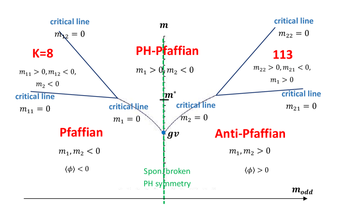
Figure 7: Phase diagram of the theory (2.1) deformed by the PH-symmetry breaking term $\delta V(\phi)=-m_{odd}\phi$ and the Majorana mass $M(m)$. Here the parameter $m$ is from the Dirac mass term in (2.1). We abbreviate $m_{11},m_{12}<0$ as $m_{1}<0$ etc. Phase boundaries can be plotted analytically by Mathematica.

2.6 Random coupling and the thermal metal phase

In the theory (2.1), we can further choose the parameter $m$ to be a random coupling with Gaussian distribution

$$\overline{m}=m_{0},\quad\overline{m^{2}}=\delta^{2}.$$ (2.27)

The theory depends on the average $m_{0}$ and the fluctuation $\delta$. In [47], it is found that for strong fluctuations $\delta\rightarrow\infty$, the system of free Dirac fermions becomes a thermal metal. We will set the magnitude of fluctuation to be

$$\delta=h(m_{0})~{}$$ (2.28)

for some non-negative, monotonically increasing function $h$ that grows faster than a linear function (for instance, $h(m_{0})=m_{0}^{2}$). Then $m_{0}$ controls the disorder strength of the system. At large enough $m_{0}$, i.e. strong disorder, the fluctuation becomes sufficiently strong and the model (2.1) with random coupling $m$ enters a thermal metal phase. Since in our model the electromagnetic background field only couples to the O(2) gauge field and does not couple to the fermions, the Hall conductivity does not depend on the mass of the fermions and remains the same value $\sigma_{xy}=\frac{5}{2}$. This is consistent with the proposal in [14, 15].

Near the critical lines of the phase diagram, the physical mass of one of the fermion becomes close to zero. If the disorder strength is nonzero for zero mass, $h(0)>0$, the disorder will cause the region sufficiently near the critical lines to have thermal metal behavior, which accommodates the behavior described in [14] and illustrated in Fig. 3.

3 Anyonic excitations and quantum observables from the EFT

Let us spell out the key properties of the TFT phases and their anyonic excitations. We assume standard knowledge from the Chern-Simons (CS) description of fQHE. We will delineate the following:

• Fractionalized anyon statistics, i.e. the spin or exchange statistics $\exp(\hskip 1.0pt\mathrm{i}\hskip 1.0pt2\pi{\rm{s}})$ of anyons with spin ${\rm{s}}$.

• Fractionalized ${\mathrm{U}}(1)_{\text{EM}}$ electromagnetic charge $Q/e$ ($e$ is the electron charge).

• Their PH-symmetry (time-reversal $CT$) transformation properties.

They are summarized in Tables 1, 2, 3, 4, and 5, for the Pfaffian, anti-Pfaffian, PH-Pfaffian, $K=8$, and 113 states respectively, in the notation

$$(\exp(\hskip 1.0pt\mathrm{i}\hskip 1.0pt2\pi{{\rm{s}}}),Q/e).$$ (3.1)

For the PH-Pfaffian, since it enjoys PH-symmetry (time-reversal $CT$), we also specify the $(CT)^{2}$ quantum number for the appropriate anyons, and write

$$(\exp(\hskip 1.0pt\mathrm{i}\hskip 1.0pt2\pi{\rm{s}}),Q/e)_{{(CT)}^{2}}.$$ (3.2)

We will first examine the non-abelian states, i.e. the Pfaffian in eqn. (2.14), anti-Pfaffian in eqn. (2.15), and PH-Pfaffian in eqn. (2.18). They can be written as the following Chern-Simons theories (see Appendix A of Ref. [15], and Appendix E):

Pfaffian $$: \quad\frac{{\mathrm{U}}(1)_{8}\times{{\text{Ising}}}}{\mathbb{Z}_{2}}-4\text{CS}_{\text{grav}},~{}\quad\;\;c_{-}=1+1/2+4/2=7/2.$$ (3.3)

PH-Pfaffian $$: \quad\frac{{\mathrm{U}}(1)_{8}\times{\overline{\text{Ising}}}}{\mathbb{Z}_{2}}-4\text{CS}_{\text{grav}},~{}\quad\;\;c_{-}=1-1/2+4/2=5/2.$$ (3.4)

anti-Pfaffian $$: \quad\frac{{\mathrm{U}}(1)_{8}\times{{\mathrm{SU}}(2)_{-2}}}{\mathbb{Z}_{2}}-4\text{CS}_{\text{grav}},~{}\;c_{-}=1-3/2+4/2=3/2.$$ (3.5)

with their chiral central charges $c_{-}=\kappa_{xy}$. These TQFTs are obtained from gauging a diagonal one-form $\mathbb{Z}_{2}$ symmetry in the (${\mathrm{U}}(1)_{8}$ CS theories) and the ($\nu\in\mathbb{Z}_{8}$-class spin-TQFTs) in 2+1$d$. More generally, these TQFTs are $\frac{{\mathrm{U}}(1)_{8}\times{T_{L}}}{\mathbb{Z}_{2}}$ for $L=-1,+1,+3$, and one gauges a diagonal $\mathbb{Z}_{2}$ one-form symmetry generated by the composite line given by the tensor product of the charge 4 Wilson line of ${\mathrm{U}}(1)_{8}$ and a non-transparent fermion line in $T_{L}$. See Appendix E for details on the $T_{L}$ theories. When gauging a diagonal $\mathbb{Z}_{2,[1]}$ symmetry, we identify their charged objects (the line with odd ${\mathrm{U}}(1)$ charge in ${\mathrm{U}}(1)_{8}$ and the $\sigma$ line in $T_{L}$) and their symmetry generators or charge operators (the operator with ${\mathrm{U}}(1)$ charge 4 in ${\mathrm{U}}(1)_{8}$ and the $f$ line in $T_{L}$). This reduces the 24 anyons in the quasi-excitation spectrum of ${{\mathrm{U}}(1)_{8}\times T_{L}}$ theory to the 12 anyons in the $\frac{{\mathrm{U}}(1)_{8}\times T_{L}}{\mathbb{Z}_{2}}$ theory.

1. Spin statistics. The spin of an anyon is given by

   $$\exp(\hskip 1.0pt\mathrm{i}\hskip 1.0pt2\pi{\rm{s}})=\exp(\hskip 1.0pt\mathrm{i}\hskip 1.0pt2\pi({\rm{s}}_{\text{nab}}+\frac{q^{2}}{2K})),$$ (3.6)

   where $K$ is the level of abelian CS theory, and $q$ is the integer labeling the abelian anyon associated with the line operator $\hskip 1.0pt\mathrm{e}^{\hskip 1.0pt\mathrm{i}\hskip 1.0ptq\oint b}$ of 1-form gauge field $b$. Here, ${\rm{s}}_{\text{nab}}$ means the spin from the non-abelian sector of the TQFT. For the Ising, $\overline{\text{Ising}}$, and ${{\mathrm{SU}}(2)_{-2}}$ TQFTs in eqn. (3.3), (3.4) and (3.5), their ${\rm{s}}_{\text{nab}}$ for the $(1,\sigma,f)$ anyons are given by the diagonal of the modular $T$ matrix: $(1,\hskip 1.0pt\mathrm{e}^{\hskip 1.0pt\mathrm{i}\hskip 1.0pt\frac{\pi}{8}},-1)$, $(1,\hskip 1.0pt\mathrm{e}^{-\hskip 1.0pt\mathrm{i}\hskip 1.0pt\frac{\pi}{8}},-1)$, and $(1,\hskip 1.0pt\mathrm{e}^{-\hskip 1.0pt\mathrm{i}\hskip 1.0pt\frac{3\pi}{8}},-1)$ respectively. See, e.g., [15] for the data.

2. Electromagnetic charge. For the anyon’s ${\mathrm{U}}(1)_{\text{EM}}$ charge $Q/e$, we can look at the coupling $q$ of the electric current to the ${\mathrm{U}}(1)_{\text{EM}}$ gauge field $A$. The charge can be changed by an integer by tensoring the line with a classical Wilson line $\oint A$. The ${\mathrm{U}}(1)_{\text{EM}}$ charge $Q$ and the Hall conductance $\sigma_{xy}$ can be computed via (see Appendix E for details):

   $$Q/e=K^{-1}q,\quad\quad\quad\sigma_{xy}=qK^{-1}q=q(Q/e).$$ (3.7)

   Based on the experimental constraint of $\sigma_{xy}=\nu=1/2$, we have to introduce the appropriate ${\mathrm{U}}(1)_{\text{EM}}$ coupling $\int\frac{2b}{2\pi}\hskip 1.0pt\mathrm{d}A=\int\frac{1}{2\pi}(2b)\hskip 1.0pt\mathrm{d}A$ to the action for the $\frac{{\mathrm{U}}(1)_{8}\times T_{L}}{\mathbb{Z}_{2}}$ theory, where the ${\mathrm{U}}(1)_{8}$ CS theory action is $\int\frac{8}{4\pi}b\hskip 1.0pt\mathrm{d}b$. This is a coupling with charge $q=2$. Indeed, this gives half-filled $\nu=\sigma_{xy}=qK^{-1}q=2^{2}/8=1/2$. The anyon with ${\mathrm{U}}(1)$-charge 2 is identified with the non-abelian $\sigma$ anyon in the gauged $\frac{{\mathrm{U}}(1)_{8}\times{T_{L}}}{\mathbb{Z}_{2}}$ CS theory. This non-abelian anyon has ${\mathrm{U}}(1)_{\text{EM}}$ charge $Q/e=K^{-1}q=2/8=1/4$. We can obtain all 12 anyons’ ${\mathrm{U}}(1)_{\text{EM}}$ charges by the same argument, with the results shown in Tables 1, 2, and 3.

3. PH-symmetry. In the PH-Pfaffian theory, PH-symmetry (or time-reversal $CT$) is preserved, so to those anyons not permuted by the time-reversal symmetry, whose spin statistics $\exp(\hskip 1.0pt\mathrm{i}\hskip 1.0pt2\pi{\rm{s}})$ are real-valued, we can assign $(CT)^{2}=\pm 1$ quantum numbers. For those anyons $\alpha_{a}$ whose spin statistics $\exp(\hskip 1.0pt\mathrm{i}\hskip 1.0pt2\pi{\rm{s}})$ are complex valued, the spin statistics are mapped to their complex conjugates $\exp(-\hskip 1.0pt\mathrm{i}\hskip 1.0pt2\pi{\rm{s}})$ under the $CT$ transformation. In fact, there are two versions of PH-Pfaffian denoted as PH-Pfaffian_± depending on how the $(CT)^{2}$ quantum number is assigned to the odd $q$ charge of ${\mathrm{U}}(1)_{8}$ anyons, which we elaborate in Table 3.

   On the other hand, the Pfaffian and anti-Pfaffian states do not have $CT$ symmetry. Instead, they map into each other under the $CT$ transformation as follows.

   • When the ${\mathrm{U}}(1)_{8}$ charge $q$ is even, the abelian sector is paired with the abelian trivial anyon 1 or the fermionic anyon $f$, so under the $CT$ transformation:

     $$\text{Pf: }(q_{\text{even}},f^{n})\overset{CT}{\Longleftrightarrow}\text{APf: }(q_{\text{even}},f^{n+\frac{q_{\text{even}}}{2}}),$$

     where $f^{2}=(f)^{\text{even}}=1$ and $n=0,1$. Namely,

     $$\text{Pf: }(q_{\text{even}},f^{n})\overset{CT}{\Longleftrightarrow}\text{APf: }(q_{\text{even}},f^{n}),\text{ if $\frac{q_{\text{even}}}{2}\in$ even}.$$

     $$\text{Pf: }(q_{\text{even}},f^{n})\overset{CT}{\Longleftrightarrow}\text{APf: }(q_{\text{even}},f^{n+1}),\text{ if $\frac{q_{\text{even}}}{2}\in$ odd}.$$

   • When the ${\mathrm{U}}(1)_{8}$ charge $q$ is odd, the abelian sector is paired with the non-abelian $\sigma$ anyon, so under $CT$:

     $$\text{Pf: }(q_{\text{odd}},\sigma)\overset{CT}{\Longleftrightarrow}\text{APf: }(q_{\text{odd}},\sigma).$$

The 12 anyons, and their spin statistics $\exp(\hskip 1.0pt\mathrm{i}\hskip 1.0pt2\pi{\rm{s}})$, ${\mathrm{U}}(1)_{\text{EM}}$ charges, and $CT$ properties are organized in Tables 1, 2, and 3. The list of anyons in the Tables contains not only quasiparticles but also quasiholes of quantum Hall liquids, to be explained in Appendix F. Although there are 12 anyons, the number of ground states on a spatial 2-torus $T^{2}$ known as the ground state degeneracy (GSD) is only 6 for the Pf, APf, and PHPf states. The corresponding 6 ground states depend on the spin structure of the spin manifold $T^{2}$.

Pfaffian	${\mathrm{U}}(1)_{8}$ CS
$T_{L=-1}$	0	1	2	3	4	5	6	7
1	$(+1,0)$		$(+\hskip 1.0pt\mathrm{i}\hskip 1.0pt,\frac{1}{2})$		$(+1,1)$		$(+\hskip 1.0pt\mathrm{i}\hskip 1.0pt,\frac{3}{2})$
$\sigma_{-1}$		$(\hskip 1.0pt\mathrm{e}^{\hskip 1.0pt\mathrm{i}\hskip 1.0pt\frac{\pi}{4}},\frac{1}{4})$		$(-\hskip 1.0pt\mathrm{e}^{\hskip 1.0pt\mathrm{i}\hskip 1.0pt\frac{\pi}{4}},\frac{3}{4})$		$(-\hskip 1.0pt\mathrm{e}^{\hskip 1.0pt\mathrm{i}\hskip 1.0pt\frac{\pi}{4}},\frac{5}{4})$		$(\hskip 1.0pt\mathrm{e}^{\hskip 1.0pt\mathrm{i}\hskip 1.0pt\frac{\pi}{4}},\frac{7}{4})$
$f$	$(-1,0)$		$(-\hskip 1.0pt\mathrm{i}\hskip 1.0pt,\frac{1}{2})$		$(-1,1)$		$(-\hskip 1.0pt\mathrm{i}\hskip 1.0pt,\frac{3}{2})$

Table 1: Pfaffian data from $\frac{{\mathrm{U}}(1)_{8}\times{\text{Ising}}}{\mathbb{Z}_{2}}$ CS. We provide $(\exp(\hskip 1.0pt\mathrm{i}\hskip 1.0pt2\pi{\rm{s}}),Q/e)$ for 12 anyons. The $\sigma_{-1}$ anyon has $\hskip 1.0pt\mathrm{e}^{\hskip 1.0pt\mathrm{i}\hskip 1.0pt\frac{\pi}{8}}$ statistics.

Anti-Pfaffian	${\mathrm{U}}(1)_{8}$ CS
$T_{L=3}$	0	1	2	3	4	5	6	7
1	$(+1,0)$		$(+\hskip 1.0pt\mathrm{i}\hskip 1.0pt,\frac{1}{2})$		$(+1,1)$		$(+\hskip 1.0pt\mathrm{i}\hskip 1.0pt,\frac{3}{2})$
$\sigma_{3}$		$(\hskip 1.0pt\mathrm{e}^{-\hskip 1.0pt\mathrm{i}\hskip 1.0pt\frac{\pi}{4}},\frac{1}{4})$		$(-\hskip 1.0pt\mathrm{e}^{-\hskip 1.0pt\mathrm{i}\hskip 1.0pt\frac{\pi}{4}},\frac{3}{4})$		$(-\hskip 1.0pt\mathrm{e}^{-\hskip 1.0pt\mathrm{i}\hskip 1.0pt\frac{\pi}{4}},\frac{5}{4})$		$(\hskip 1.0pt\mathrm{e}^{-\hskip 1.0pt\mathrm{i}\hskip 1.0pt\frac{\pi}{4}},\frac{7}{4})$
$f$	$(-1,0)$		$(-\hskip 1.0pt\mathrm{i}\hskip 1.0pt,\frac{1}{2})$		$(-1,1)$		$(-\hskip 1.0pt\mathrm{i}\hskip 1.0pt,\frac{3}{2})$

Table 2: Anti-Pfaffian data from the $\frac{{\mathrm{U}}(1)_{8}\times{{\mathrm{SU}}(2)_{-2}}}{\mathbb{Z}_{2}}$ CS. We provide $(\exp(\hskip 1.0pt\mathrm{i}\hskip 1.0pt2\pi{\rm{s}}),Q/e)$ for 12 anyons. The $\sigma_{3}$ anyon has $\hskip 1.0pt\mathrm{e}^{-\hskip 1.0pt\mathrm{i}\hskip 1.0pt\frac{3\pi}{8}}$ statistics.

PH-Pfaffian±	${\mathrm{U}}(1)_{8}$ CS
$T_{L=1}$	0	1	2	3	4	5	6	7
1	$(+1,0)_{1}$		$(+\hskip 1.0pt\mathrm{i}\hskip 1.0pt,\frac{1}{2})$		$(+1,1)_{-1}$		$(+\hskip 1.0pt\mathrm{i}\hskip 1.0pt,\frac{3}{2})$
$\sigma_{1}$		$(1,\frac{1}{4})_{\pm 1}$		$(-1,\frac{3}{4})_{\mp 1}$		$(-1,\frac{5}{4})_{\mp 1}$		$(1,\frac{7}{4})_{\pm 1}$
$f$	$(-1,0)_{1}$		$(-\hskip 1.0pt\mathrm{i}\hskip 1.0pt,\frac{1}{2})$		$(-1,1)_{-1}$		$(-\hskip 1.0pt\mathrm{i}\hskip 1.0pt,\frac{3}{2})$

Table 3: PH-Pfaffian data from $\frac{{\mathrm{U}}(1)_{8}\times\overline{\text{Ising}}}{\mathbb{Z}_{2}}$ CS. We provide $(\exp(\hskip 1.0pt\mathrm{i}\hskip 1.0pt2\pi{\rm{s}}),Q/e)$ or $(\exp(\hskip 1.0pt\mathrm{i}\hskip 1.0pt2\pi s),Q/e)_{(CT)^{2}}$ for 12 anyons. The $\sigma_{1}$ anyon has $\hskip 1.0pt\mathrm{e}^{-\hskip 1.0pt\mathrm{i}\hskip 1.0pt\frac{\pi}{8}}$ statistics. In comparison, Ref. [17] represents related TQFT data in terms of $\frac{{\mathrm{U}}(1)_{-8}\times{\text{Ising}}}{\mathbb{Z}_{2}}$ CS. Moreover, there are two versions PH-Pfaffian_± depending on how $(CT)^{2}$ assigns to the odd $q=1,3,5,7$ of ${\mathrm{U}}(1)_{8}$.

Now we examine the abelian states. The $K=8$ state in eqn. (2.25) has the action $\int\frac{8}{4\pi}b\hskip 1.0pt\mathrm{d}b+\frac{2b}{2\pi}\hskip 1.0pt\mathrm{d}A-4\text{CS}_{\text{grav}}$ plus a trivial spin-TQFT with $\{1,f\}$ (generated by a trivial line and a fermionic line). Note that the fermion $f$ does not couple to ${\mathrm{U}}(1)_{\text{EM}}$.

The $113$ state in eqn. (2.26) has the action $\frac{K_{IJ}}{4\pi}\int b_{I}\hskip 1.0pt\mathrm{d}b_{J}+\frac{(q^{{\rm T}}_{I}\cdot b_{I})}{2\pi}\hskip 1.0pt\mathrm{d}A-4\text{CS}_{\text{grav}},$ where $q^{\rm{T}}$ denotes the transpose of the $q$ charge vector. There are two convenient expressions for this theory, related by a GL(2,$\mathbb{Z}$) transformation [15]:

$$K=\left(\begin{array}[]{cc}1&3\\ 3&1\end{array}\right),q^{\rm{T}}=(1,1)\;{\xleftrightarrow{\text{GL(2,$\mathbb{Z}$) transformation}}}\;K=\left(\begin{array}[]{cc}-8&0\\ 0&1\end{array}\right),q^{\rm{T}}=(2,1).$$

(We omit an electron charge normalization factor $e$.)

The quantum numbers for the abelian states are shown in Tables 4 and Table 5. The spin statistics can be obtained from eqn. (3.6) by dropping the ${\rm{s}}_{\text{nab}}$ part. The ${\mathrm{U}}(1)_{\text{EM}}$ charge can be determined from eqn. (3.7) as before.

$K=8$-state	${\mathrm{U}}(1)_{8}$ CS
$T_{L=0}$	0	1	2	3	4	5	6	7
1	$(+1,0)$	$(\hskip 1.0pt\mathrm{e}^{\hskip 1.0pt\mathrm{i}\hskip 1.0pt\frac{\pi}{8}},\frac{1}{4})$	$(\hskip 1.0pt\mathrm{e}^{\hskip 1.0pt\mathrm{i}\hskip 1.0pt\frac{\pi}{2}},\frac{1}{2})$	$(-\hskip 1.0pt\mathrm{e}^{\hskip 1.0pt\mathrm{i}\hskip 1.0pt\frac{\pi}{8}},\frac{3}{4})$	$(+1,1)$	$(-\hskip 1.0pt\mathrm{e}^{\hskip 1.0pt\mathrm{i}\hskip 1.0pt\frac{\pi}{8}},\frac{5}{4})$	$(\hskip 1.0pt\mathrm{e}^{\hskip 1.0pt\mathrm{i}\hskip 1.0pt\frac{\pi}{2}},\frac{3}{2})$	$(\hskip 1.0pt\mathrm{e}^{\hskip 1.0pt\mathrm{i}\hskip 1.0pt\frac{\pi}{8}},\frac{7}{4})$
$f$	$(-1,0)$	$(-\hskip 1.0pt\mathrm{e}^{\hskip 1.0pt\mathrm{i}\hskip 1.0pt\frac{\pi}{8}},\frac{1}{4})$	$(-\hskip 1.0pt\mathrm{e}^{\hskip 1.0pt\mathrm{i}\hskip 1.0pt\frac{\pi}{2}},\frac{1}{2})$	$(\hskip 1.0pt\mathrm{e}^{\hskip 1.0pt\mathrm{i}\hskip 1.0pt\frac{\pi}{8}},\frac{3}{4})$	$(-1,1)$	$(\hskip 1.0pt\mathrm{e}^{\hskip 1.0pt\mathrm{i}\hskip 1.0pt\frac{\pi}{8}},\frac{5}{4})$	$(-\hskip 1.0pt\mathrm{e}^{\hskip 1.0pt\mathrm{i}\hskip 1.0pt\frac{\pi}{2}},\frac{3}{2})$	$(-\hskip 1.0pt\mathrm{e}^{\hskip 1.0pt\mathrm{i}\hskip 1.0pt\frac{\pi}{8}},\frac{7}{4})$

Table 4: Data for the $K=8$-state. We provide $(\exp(\hskip 1.0pt\mathrm{i}\hskip 1.0pt2\pi{\rm{s}}),Q/e)$ for 16 anyons.

113-state	${\mathrm{U}}(1)_{-8}$ CS
$T_{L=2}$	0	1	2	3	4	5	6	7
1	$(+1,0)$	$(\hskip 1.0pt\mathrm{e}^{-\hskip 1.0pt\mathrm{i}\hskip 1.0pt\frac{\pi}{8}},\frac{7}{4})$	$(\hskip 1.0pt\mathrm{e}^{-\hskip 1.0pt\mathrm{i}\hskip 1.0pt\frac{\pi}{2}},\frac{3}{2})$	$(-\hskip 1.0pt\mathrm{e}^{-\hskip 1.0pt\mathrm{i}\hskip 1.0pt\frac{\pi}{8}},\frac{5}{4})$	$(+1,1)$	$(-\hskip 1.0pt\mathrm{e}^{-\hskip 1.0pt\mathrm{i}\hskip 1.0pt\frac{\pi}{8}},\frac{3}{4})$	$(\hskip 1.0pt\mathrm{e}^{-\hskip 1.0pt\mathrm{i}\hskip 1.0pt\frac{\pi}{2}},\frac{1}{2})$	$(\hskip 1.0pt\mathrm{e}^{-\hskip 1.0pt\mathrm{i}\hskip 1.0pt\frac{\pi}{8}},\frac{1}{4})$
$f$	$(-1,1)$	$(-\hskip 1.0pt\mathrm{e}^{-\hskip 1.0pt\mathrm{i}\hskip 1.0pt\frac{\pi}{8}},\frac{3}{4})$	$(-\hskip 1.0pt\mathrm{e}^{-\hskip 1.0pt\mathrm{i}\hskip 1.0pt\frac{\pi}{2}},\frac{1}{2})$	$(\hskip 1.0pt\mathrm{e}^{-\hskip 1.0pt\mathrm{i}\hskip 1.0pt\frac{\pi}{8}},\frac{1}{4})$	$(-1,0)$	$(\hskip 1.0pt\mathrm{e}^{-\hskip 1.0pt\mathrm{i}\hskip 1.0pt\frac{\pi}{8}},\frac{7}{4})$	$(-\hskip 1.0pt\mathrm{e}^{-\hskip 1.0pt\mathrm{i}\hskip 1.0pt\frac{\pi}{2}},\frac{3}{2})$	$(-\hskip 1.0pt\mathrm{e}^{-\hskip 1.0pt\mathrm{i}\hskip 1.0pt\frac{\pi}{8}},\frac{5}{4})$

Table 5: Data for the 113-state. We provide $(\exp(\hskip 1.0pt\mathrm{i}\hskip 1.0pt2\pi{\rm{s}}),Q/e)$ for 16 anyons.

The $K=8$ and 113-states do not have $CT$ symmetry. Instead, they map into each other under the $CT$ transformation. Quantum numbers of their anyons are mapped as:

$$K=8:\quad(\exp(\hskip 1.0pt\mathrm{i}\hskip 1.0pt2\pi{\rm{s}}),Q/e\mod 1)\overset{CT}{\Longleftrightarrow}113:\quad(\exp(-\hskip 1.0pt\mathrm{i}\hskip 1.0pt2\pi{\rm{s}}),Q/e\mod 1).$$

The mod 1 comes from the freedom to tensor the anyons with the classical Wilson line $\oint A$.

Although there are 16 anyons in each the abelian state, the GSD is only 8. The corresponding 8 ground states depend on the spin structure of the spin manifold 2-torus $T^{2}$.

4 Domain wall theory and tension

As reviewed in the introduction, the proposal of [15] suggests a percolation transition involving puddles of Pf and APf phases separated by domain walls. To this end, we consider the model (2.1) on the slice of parameter space with time-reversal symmetry preserved, i.e. $m_{odd}=0$. We would like to study some basic properties of the domain walls, from the EFT point of view, that result when time-reversal symmetry is spontaneously broken.

Let us ignore the discrete gauge field which couples to the fermions, for now, and write the Lagrangian as (in the mostly positive Lorentzian signature)

$${\cal L}=\sum_{i=1,2}\overline{\Psi}^{i}(\hskip 1.0pt\mathrm{i}\hskip 1.0pt{\ooalign{\hfil\hfil/\hfil\cr$D$}}-g\phi)\Psi^{i}+m(\overline{\Psi}^{1}\Psi^{1}-\overline{\Psi}^{2}\Psi^{2})+{1\over 2}(\partial_{\mu}\phi)(\partial^{\mu}\phi)-{1\over 4}\lambda(\phi^{2}-v^{2})^{2}.$$ (4.1)

The vacua are doubly degenerate, with the vevs given by $\pm v$ where $v\equiv{\mu/\sqrt{\lambda}}$. Throughout this section, we assume without loss of generality that $m,\,g\geq 0$.

The classical solution for a static domain wall is, as usual,

$$\phi_{0}(z)={\mu\over\sqrt{\lambda}}\tanh{\mu(z-z_{0})\over\sqrt{2}}$$ (4.2)

with $z_{0}$ the center-of-mass coordinate. We assume that the effective perturbative expansion parameter in the scalar sector, $\lambda/\mu$, is small to validate the semiclassical analysis that we perform presently. The classical action evaluated on the domain wall saddle is

$$S_{\phi}[\phi_{0}]={2\sqrt{2}\over 3}{\mu^{3}\over\lambda}\int\hskip 1.0pt\mathrm{d}^{2}x\,,$$ (4.3)

where $\hskip 1.0pt\mathrm{d}^{2}x$ is over the parallel directions to the domain wall, and the transverse $z$ direction has already been integrated over. Divided by the area worldvolume area $\int\hskip 1.0pt\mathrm{d}^{2}x$, this famously gives the classical domain wall tension [51, 52]

$$\sigma_{cl}={2\sqrt{2}\over 3}{\mu^{3}\over\lambda}.$$ (4.4)

For nonzero fermion mass, the two vacua are gapped. At energies smaller than the $2+1d$ bulk gap, we have well-defined 1+1$d$ domain wall theories. To derive the domain wall theories, we first analyze the fermionic zero modes (which survive the low energy limit) in section 4.1, and then proceed to quantize the zero modes to obtain the domain wall theories in section 4.2. We then study another aspect of the domain walls – their tension, and we do so at one-loop order.

4.1 Fermionic zero modes in the domain wall background

In the semiclassical approximation, the transverse profile of fermion modes solves the Dirac equation in the domain wall background:

$$(\epsilon_{r}\gamma^{0}+\hskip 1.0pt\mathrm{i}\hskip 1.0pt\gamma^{1}{\partial\over\partial z}\pm m-g\phi_{0}(z))\Psi^{j}_{0}(z)=0.$$ (4.5)

We have, for the moment, suppressed dependence on the spatial direction parallel to the domain wall. We use the Majorana basis for $\Gamma$-matrices $\gamma^{0}=-\hskip 1.0pt\mathrm{i}\hskip 1.0pt\sigma^{y},\gamma^{1}=\sigma^{z},\gamma^{2}=\sigma^{x}$, and write the two-component spinors explicitly as $\Psi^{j}(z)=(u^{j}_{r}(z),v^{j}_{r}(z))^{{\rm T}}$, $j=1,2$ (so the top component is of definite chirality and the bottom component has the opposite chirality). With these conventions, the above equation becomes

$$(-{\partial\over\partial z}\pm m-g\phi_{0}(z))v^{j}_{r} =\epsilon_{r}u^{j}_{r}(z),$$

$$({\partial\over\partial z}\pm m-g\phi_{0}(z))u^{j}_{r} =-\epsilon_{r}v^{j}_{r}(z).$$

We are interested in the zero-modes, which survive the low energy limit. For $\epsilon_{0}=0$, we can solve these equations in the classical domain wall background:

$$u^{1}_{0}(z) =\psi^{1}_{0,+}\hskip 1.0pt\mathrm{e}^{-m(z-z_{0})}\cosh\left((z-z_{0}){\mu\over\sqrt{2}}\right)^{\sqrt{2}g\over\sqrt{\lambda}},$$ (4.6)

$$v^{1}_{0}(z) =\psi^{1}_{0,-}e^{m(z-z_{0})}\cosh\left((z-z_{0}){\mu\over\sqrt{2}}\right)^{-\sqrt{2}g\over\sqrt{\lambda}},$$ (4.7)

and

$$u^{2}_{0}(z) =\psi^{2}_{0,+}\hskip 1.0pt\mathrm{e}^{m(z-z_{0})}\cosh\left((z-z_{0}){\mu\over\sqrt{2}}\right)^{\sqrt{2}g\over\sqrt{\lambda}},$$ (4.8)

$$v^{2}_{0}(z) =\psi^{2}_{0,-}\hskip 1.0pt\mathrm{e}^{-m(z-z_{0})}\cosh\left((z-z_{0}){\mu\over\sqrt{2}}\right)^{-\sqrt{2}g\over\sqrt{\lambda}}.$$ (4.9)

Let us discuss the properties of the zero modes in the Pfaffian/anti-Pfaffian regime $m<gv$ and the PH-Pfaffian regime $m>gv$. These properties will be the key in our subsequent determination of the respective domain wall theories in section 4.2.

When $m<gv$, since the solution for $u^{j}_{0}(z),j=1,2$ is not normalizable, we set both $\psi^{j}_{0,+}=0$ and are therefore left with two complex parameters $\psi^{j}_{0,-}$, which constitute our expected four real fermionic zero modes of a single chirality (thus, they correspond to four chiral Majorana fermions). In the extreme limit of $m\ll gv$, the zero-modes satisfy $\overline{\Psi}\Psi\sim\Psi^{\dagger}\sigma_{2}\Psi=0$, and hence do not backreact on the scalar via the equations of motion.

When $m>gv$, the fermions delocalize and are essentially described by plane wave solutions. For each Dirac fermion, the normalizable edge modes of opposite chiralities survive on different sides of a half-space:

Fermion	$z\geq z_{0}$	$z\leq z_{0}$
$\Psi^{1}$ (mass $m>0$)	$\psi^{1}_{-}$	$\psi^{1}_{+}$
$\Psi^{2}$ (mass $-m<0$)	$\psi^{2}_{+}$	$\psi^{2}_{-}$

The semiclassical limit $\mu/\lambda\gg 1$ is also a “hard-wall” limit, in which the soliton solution tends towards a steep step-function at $z=z_{0}$ with an insurmountable height barrier. Then we can indeed consider the normalizable edge modes on two half-spaces that can only interact via possible couplings on the interface. Among the relevant interactions, a 1+1$d$ Majorana mass term for each fermion species, induced from the bulk mass term, can survive precisely on the wall, and gaps out the fermionic degrees of freedom at low energies. This is rather analogous to wall-localized supersymmetric couplings that appear in [53].

4.2 Domain wall worldvolume theory in $1+1d$

There is a natural proposal for the domain wall worldvolume theory following from simple anomaly considerations. It is the O(2) WZW model coupled to two massless complex Dirac fermions by a common $\mathbb{Z}_{2}$ orbifold that acts as the charge conjugation in O(2). The chiral anomaly accounts for the relative shift of the Chern-Simons level in the two bulk vacua. Since the U(1) part of the gauge field is confined in 1+1$d$, the theory naturally flows to $\mathbb{Z}_{2}$ coupled to two complex fermions. The domain wall theory has ${\mathrm{O}}(4)/\mathbb{Z}_{2}$ symmetry which rotates the four massless real fermions. This is consistent with the proposal in [15].

Let us now derive the domain wall worldvolume theory from first principles to verify this intuition. For the moment, we will ignore the presence of the discrete gauge field, and reinstate its effect at the end. The vacua, which spontaneously break the time-reversal invariance, occur at $\langle\phi\rangle=\pm v$. The fermions in each of these vacua have tree-level masses $\pm m+g\langle\phi\rangle=\pm m\pm gv$.

To get the 1+1$d$ domain wall theories, we wish to quantize the zero-modes in the two regimes of interest, $m<gv$ and $m>gv$. We first describe a sector of the worldvolume theory without fermions, and then describe the interesting fermionic sector alluded to above. In the following, all quantities are the renormalized versions, as we imagine having already integrated out the bulk massive modes.

Goldstone mode

Since the domain wall breaks translational invariance, there is an effective action for the bosonic Goldstone center-of-mass mode. It arises from promoting the modulus $z_{0}$ $\in{\mathbb{R}}$ adiabatically to functions of the worldvolume directions $m\in(t,x)$. Integrating over $z$ and dropping a standard additive constant (hence our use of $\sim$ below) gives

$$\mathcal{L}^{G}[z_{0}]={1\over 2}\int\hskip 1.0pt\mathrm{d}z\left((\partial_{z}\phi_{0})^{2}+(\partial_{m}z_{0}(x,t)\partial_{z}\phi_{0})^{2}\right)\sim{\sigma_{cl}\over 2}(\partial_{m}z_{0}(x,t))^{2},$$ (4.10)

where the bosonic tension is

$$\sigma_{cl}={2\sqrt{2}\over 3}{\mu^{3}\over\lambda},$$ (4.11)

in agreement with the tension (4.4) derived from evaluating the classical (effective) action on the domain wall solution. We neglect irrelevant higher-derivative terms in the fluctuation $z_{0}(x,t)$.

Wess-Zumino-Witten (WZW) models

Since the Chern-Simons sector of the bulk theory does not interact with the degrees of freedom on the wall except via the $\mathbb{Z}_{2}$ gauging of the fermions, the domain wall is transparent to the continuous gauge degrees of freedom. As is well known, the 1+1$d$ theory that furnishes a trivial interface for a Chern-Simons gauge field is the corresponding WZW theory.

This bulk Chern-Simons term on the two sides of the wall contributes a diagonal CFT on the wall due to the opposite orientations with respect to the bulk. The theory on the wall can be constructed as follows. First we start with the bulk theory ${\mathrm{SO}}(2)_{2}={\mathrm{U}}(1)_{2}$ on both sides of the wall, so that the theory on the wall is naturally a compact boson at the self-dual radius. Then we deposit additional $L$ units of $\mathbb{Z}_{2}$ SPT phases in the bulk, which induce additional fermions on the wall. The amount $L$ of $\mathbb{Z}_{2}$ SPT phases appropriate for each phase was discussed in Section 2.3, which we summarize here for the convenience of the reader:

Phase	$L$
PH-Pfaffian	$1$
Pfaffian	$-1$
Anti-Pfaffian	$3\equiv-5\mod 8$

Finally, we gauge the diagonal $\mathbb{Z}_{2}$ symmetry of the entire configuration that acts as charge conjugation on the ${\mathrm{SO}}(2)$ gauge field. This introduces a single $\mathbb{Z}_{2}$ gauge field throughout the bulk and on the wall. In other words, at the interface we identify the $\mathbb{Z}_{2}$ gauge field on the left side of the wall with the gauge field on the right. We may employ the relation among Chern-Simons theories

$${\mathrm{SO}}(2)_{2}\xrightarrow{\text{gauging $\mathbb{Z}_{2}$}}{\mathrm{O}}(2)_{2,L}={{\mathrm{U}}(1)_{8}\times T_{L}\over\mathbb{Z}_{2}}$$ (4.12)

where the theories $T_{L},~{}L\textrm{ mod }8$ are described in Appendix E.

In the PH-Pfaffian regime, we have $L=1$, and the contribution from the bulk on one side is given by gauging a diagonal $\mathbb{Z}_{2}$ symmetry in the product of a left-moving compact boson $\varphi$ at the self dual radius and a right-moving Majorana fermion $\zeta^{R}$. The contribution from the other side of the wall is the same with left exchanged with right. Of course, the chiral anomaly of this sector from both sides of the wall is trivial.

In the Pfaffian/anti-Pfaffian regime, an interface interpolating between the Pfaffian and anti-Pfaffian WZW theories differs from this basic one ($L=1$) by precisely four additional Majorana fermions of the same chirality. On the Pfaffian side of the wall we have a left-moving compact boson and a left-moving Majorana fermion, while on the anti-Pfaffian side we have a right-moving compact boson and five right-moving fermions as appropriate for the theories with $L=-1,(3\equiv-5)$, respectively. Both sides are again gauged by a single $\mathbb{Z}_{2}$ gauge field. We denote the discrete $\mathbb{Z}_{2}$ gauge field below as $a$, which implements a projection on the spectrum — on the $\Psi^{j}$ as well as $\varphi,\zeta$.

Therefore, the domain wall theory before the contribution of the SPT-induced fermions is

$$S^{G}[z_{0}]+S^{{WZW}}[a,\zeta,\varphi]$$ (4.13)

in the obvious notation, where the superscript $WZW$ denotes the appropriate WZW model for a given phase. The theory for the fermions that the SPT phases deposit on the wall will now be derived using our previous analysis of bulk fermionic zero modes in Section 4.1.

Fermionic sector

Let us study the Pfaffian/anti-Pfaffian regime $m<gv$ in the extreme limit of $m=0$. We take the normalizable zero-modes $\psi_{0,-}$ and promote them to worldvolume fields. We substitute the corresponding solutions in terms of two complex Weyl fermions (4.6, 4.8) into the Lagrangian (4.1) to obtain

$$\mathcal{L}^{\text{Pf/APf}}[a,\Psi]\sim\widetilde{\sigma}\sum_{i=1,2}\overline{\psi}^{i}_{0,-}(x,t)({\hskip 1.0pt\mathrm{i}\hskip 1.0pt}{\ooalign{\hfil\hfil/\hfil\cr$D$}}_{a})\psi^{i}_{0,-}(x,t),$$ (4.14)

where all derivatives only run over the worldvolume coordinates $k=x,t$, and we have used the superscript to indicate that this is the domain wall theory that interpolates between the Pfaffian and anti-Pfaffian vacua. The coefficient of the kinetic term $\widetilde{\sigma}$ is given by the integral

$$\widetilde{\sigma}=\int_{-\infty}^{\infty}\hskip 1.0pt\mathrm{d}z\cosh(\mu(z-z_{0})/\sqrt{2})^{-{2\sqrt{2}g\over\sqrt{\lambda}}}={\sqrt{2\pi}\over\mu}{\Gamma({\sqrt{2}g\over\sqrt{\lambda}})\over\Gamma({1\over 2}+{\sqrt{2}g\over\sqrt{\lambda}})},$$ (4.15)

which in the limit of small Yukawa coupling becomes

$$\widetilde{\sigma}\sim{\sqrt{\lambda}\over\mu g}.$$ (4.16)

The gauge field couples to the fermions on the wall exactly as it did in the bulk. Note that the WZW sector is almost decoupled from the fermions except for the $\mathbb{Z}_{2}$ gauging.

In the PH-Pfaffian regime $m>gv$, let us set $g=0$ for simplicity, and use the plane wave solutions on opposite sides of the walls. Doing the respective integrals for the surviving zero-modes over the two half-spaces ($z\leq z_{0},z\geq z_{0}$) then gives

$$\mathcal{L}^{\text{PHPf}}[a,\Psi]$$

$$={m\over\mu}\left[\psi^{1}_{0,+}(x,t)\psi^{1}_{0,-}(x,t)-\psi^{2}_{0,+}(x,t)\psi^{2}_{0,-}(x,t)\right]+{1\over 2m}\sum_{i=1,2}\overline{\psi}^{i}_{0}(x,t)({\hskip 1.0pt\mathrm{i}\hskip 1.0pt}{\ooalign{\hfil\hfil/\hfil\cr$D$}}_{a})\psi^{i}_{0}(x,t)\,,$$ (4.19)

where now the superscript indicates that the domain wall theory is for the PH-Pfaffian phase. The mass term gaps out the fermions at low energies, hence only the Goldstone and WZW sectors of the domain wall theory survives on the wall.

The analysis of the zero modes in the two extreme regimes also suggests a natural candidate domain wall theory (in the universality class of the theory) that describes the wall’s phase transition: a 1+1$d$ $\mathbb{Z}_{2}$-gauged Gross-Neveu-Yukawa theory (suppressing the dependence of the fields on the worldvolume coordinates $(x,t)$)

$$\mathcal{L}^{wall}=-{1\over 2}(\partial\varphi)^{2}+g_{2}^{2}\varphi^{2}-{g_{4}\over 4}\varphi^{4}-g_{3}\phi\left(\overline{\psi}^{1}\psi^{1}-\overline{\psi^{2}}\psi^{2}\right)+\sum_{j}\overline{\psi}^{j}({\hskip 1.0pt\mathrm{i}\hskip 1.0pt}{\ooalign{\hfil\hfil/\hfil\cr$D$}}_{a})\psi^{j}.$$ (4.20)

Here, the condensation of the scalar $\sigma$ as we tune the scalar mass term implements the phase transition between the two regimes. If we canonically normalize the fermions in $\mathcal{L}^{\text{PHPf}}$, then the coefficient of the mass term becomes ${m^{2}\over\mu}$, so that we set ${m^{2}\over\mu}\sim{g_{3}g_{2}\over\sqrt{g_{4}}}$, which naively suggests $g_{4}\sim\mu^{2},g_{3}\sim g_{2}\sim m$. We defer a more detailed analysis for future work.

4.3 One-loop effective action and tension

Let us return to our $2+1d$ bulk theory and study the (Euclidean) effective action and the domain wall tension from integrating out fermions at one-loop. We ignore the $\mathbb{Z}_{2}$ gauging and revisit its effect towards the end.

Consider expanding the theory in transverse fluctuations around a saddle $\phi=\phi_{0}+\chi$, where $\phi_{0}$ could be either the vacuum saddle $\phi_{0}=\pm v$ or the domain wall saddle (4.2). The matter part of the action then takes the form

$$S_{bulk}={2\sqrt{2}\over 3}{\mu^{3}\over\lambda}+S_{fluct}+S_{ct},$$ (4.21)

where (suppressing the $2+1$d spacetime dependence of the fields)

$$S_{fluct} =\int\hskip 1.0pt\mathrm{d}^{3}x\,{1\over 2}\left\{\chi\left(-{\partial^{2}\over\partial z^{2}}-\mu^{2}+3\lambda\phi_{0}^{2}\right)\chi+\lambda\left(\phi_{0}\chi^{3}+{1\over 4}\chi^{4}\right)\right\}$$ (4.22)

$$+\sum_{i=1,2}\overline{\Psi}^{i}\hskip 1.0pt\mathrm{i}\hskip 1.0pt{\ooalign{\hfil\hfil/\hfil\cr$D$}}_{\cal C}\Psi^{i}++m(\overline{\Psi}^{1}\Psi^{1}-\overline{\Psi}^{2}\Psi^{2})+\int dz\left\{-g\sum_{i=1,2}(\phi_{0}+\chi)\overline{\Psi}^{i}\Psi^{i}\right\}$$

is the action for the fluctuations. We will study the counterterms $S_{ct}$ below.

4.3.1 Effective action at $\phi_{0}=v$

At one-loop order around the vacuum saddle $\phi_{0}=v$, there are terms in the fluctuation action that contribute to $\langle\chi\rangle$ via tadpole diagrams:

$$-g\chi\overline{\Psi}^{i}\Psi^{i}+\lambda v\chi^{3}.$$ (4.23)

We need to include counterterms to cancel the tadpole so that the location of the vacuum remains fixed, $\langle\phi\rangle=v$. Explicitly,

$$S_{ct} =-{1\over 2}\delta_{b}\mu^{2}\int\hskip 1.0pt\mathrm{d}^{3}x\,\phi^{2}-{1\over 2}\delta_{f}\mu^{2}\int\hskip 1.0pt\mathrm{d}^{3}x\,\phi^{2}\,,$$ (4.24)

$$\delta_{b}\mu^{2} =\lambda v\int^{\Lambda}{\hskip 1.0pt\mathrm{d}^{3}k\over(2\pi)^{3}}{1\over k^{2}+\mu^{2}}\,,$$

$$\delta_{f}\mu^{2} =2g\int^{\Lambda}{\hskip 1.0pt\mathrm{d}^{3}k\over(2\pi)^{3}}\left[{g+m/v\over k^{2}+(gv+m)^{2}}+{g-m/v\over k^{2}+(gv-m)^{2}}\right]\,,$$

where $\delta_{b}$ and $\delta_{f}$ denote counterterms that arise from consideration of bosonic $\chi$ and fermionic $\Psi^{i}$ loops, respectively, and $\Lambda$ is a UV cutoff.

Figure 8: Fermionic one-loop renormalization of the fluctuating scalar mass.

The mass of the fluctuating $\chi$ field is given by $\sqrt{2}\mu$ at tree level, but gets corrected at one-loop, with the Feynman diagram given in Figure 8. Since we want to focus on the effect of the fermions, let us ignore the bosonic loop corrections for now. The one-loop effective action from integrating out two Dirac fermions with masses $\pm m$ and coupled to the scalar with Yukawa coupling $g$ is

$$\delta_{f}{\cal L}_{eff}=\log{\det\mathbb{D}_{m,g}^{\phi=v+\chi}\over\det\mathbb{D}_{m,g}^{\phi=v}}{\det\mathbb{D}_{-m,g}^{\phi=v+\chi}\over\det\mathbb{D}_{-m,g}^{\phi=v}}-{1\over 2}\delta_{f}\mu^{2}\left[(v+\chi)^{2}-v^{2}\right]\,,$$ (4.25)

where $\mathbb{D}_{m,g}^{\phi}$ is the effective Dirac operator

$$\mathbb{D}_{m,g}^{\phi}\equiv\begin{pmatrix}\displaystyle-\partial_{1}+m+gv+g\chi&-\hskip 1.0pt\mathrm{i}\hskip 1.0pt\partial_{0}-\partial_{2}\\ i\partial_{0}-\partial_{2}&\displaystyle\partial_{1}+m+gv+g\chi&\end{pmatrix}\,.$$ (4.26)

When $m\neq gv$, the leading terms in the derivative expansion amount to treating $\chi$ as a constant,

$$\delta_{f}{\cal L}_{eff} =\int{\hskip 1.0pt\mathrm{d}^{3}k\over(2\pi)^{3}}\Bigg{\{}\log{k^{2}+(m+gv+g\chi)^{2}\over k^{2}+(m+gv)^{2}}\,{k^{2}+(m-gv-g\chi)^{2}\over k^{2}+(m-gv)^{2}}$$ (4.27)

$$\hskip 36.135pt-g[(v+\chi)^{2}-v^{2}]\left[{g+m/v\over k^{2}+(m+gv)^{2}}+{g-m/v\over k^{2}+(m-gv)^{2}}\right]\Bigg{\}}$$

$$=\begin{cases}\displaystyle-{g^{2}v^{2}-m^{2}\over 2\pi|gv|}(g\chi)^{2}-{1\over 3\pi}(g\chi)^{3}&m<gv\,,\\ \displaystyle-{1\over 6\pi}(g\chi)^{3}&m=gv\,,\\ 0&m>gv\,.\end{cases}$$

We see that the mass of $\chi$ is renormalized as

$$2\mu^{2}=2\mu_{cl}^{2}+{g^{2}v^{2}-m^{2}\over\pi|gv|}g^{2}\theta(g^{2}v^{2}-m^{2})\,,\quad v={\mu\over\sqrt{\lambda}}\,.$$ (4.28)

In what regime can we trust this result? Let us estimate this by computing some higher derivative terms in the one-loop effective action. For a single Dirac fermion with mass $\overline{m}$, the first few higher derivative corrections quadratic in $\chi$ are

$$\delta_{f}S_{eff}^{(2)} =-{g^{2}\over 2}\chi\left({1\over 12\pi|m-gv|}\partial^{2}+{1\over 240\pi|m-gv|^{3}}\,\partial^{4}+{\cal O}(\partial^{6})\right)\chi+{\cal O}(\chi^{3})\,,$$ (4.29)

with some computational details given in Appendix G.1. Estimating the $\partial^{2}$ for bosonic fluctuations by the mass $\sqrt{2}\mu$, we find that the higher derivative corrections are suppressed by factors of ${|m-gv|/\mu}$. Thus our result is a reasonable approximation in the regime

$${|m-gv|\over\mu}\gtrsim{\cal O}(1)\,.$$ (4.30)

We will come back to this at the end of Section 4.3.2.

4.3.2 Domain wall tension

To evaluate the one-loop corrections to the tension, we will closely follow the method of [56] (see also [57]). First, we formulate the theory in a Euclidean box with half-length $L$ in the $z$ direction and area $V_{||}$ in the worldvolume directions, so that the energy density is given in terms of the effective action $\Gamma$ as

$$\sigma=\textrm{lim}_{L,V_{||}\rightarrow\infty}{\Gamma(\phi_{0})\over V_{||}}\,,$$ (4.31)

under a scheme such that the expectation values of the vacua $\pm v$ are unrenormalized, and the effective action is normalized to vanish when evaluated on the vacua $\pm v$.

Formally, the full one-loop correction to this quantity receives contributions from the classical term $\sigma_{cl}$ (taking the form of (4.4) with $\mu$ renormalized), the quantum correction $\sigma_{qu}$, and the counterterms $\sigma_{ct}$:

$$\sigma =\sigma_{cl}+\sigma_{qu}+\sigma_{ct}$$ (4.32)

$$=\int\hskip 1.0pt\mathrm{d}z\left(\mathcal{L}(\phi_{0})-\mathcal{L}(v)\right)+\textrm{lim}_{L,V_{||}\rightarrow\infty}\left({1\over 2V_{||}}\textrm{ln det}{\Delta\over\Delta^{(0)}}\right)\,.$$ (4.33)

The operators $\Delta,\Delta^{(0)}$ are the inverse propagators of a fluctuating field in the soliton background and in the vacuum (trivial background), respectively. The central idea of [56] is that the fluctuations are independent of the worldvolume coordinates and may therefore be partially diagonalized by a Fourier transform in those directions. Then, the ratio of functional determinants can be related to a ratio of solutions of ordinary differential equations, which is then (numerically) integrated over the transverse coordinates.

First, we express the one-loop tension in terms of the renormalized parameters of the theory. As is standard [58, 64, 56], the renormalized scalar mass $\mu$ can be related to the bare mass $\mu_{bare}$ by a one-loop computation in the perturbative sector of the fluctuation theory, i.e. in one of the two degenerate ground states. We follow [56] and use the $\overline{\textrm{MS}}$ scheme to fix the counterterms, and require that, as discussed above, the tadpole diagrams are cancelled by the counterterms. This coincides with the condition to fix the renormalized mass by requiring $\langle\phi\rangle=\pm\sqrt{6\mu^{2}/\lambda}$.

The full one-loop tension can be broken up into a sum of the classical tension and the bosonic and fermionic one-loop contributions, of the form

$$\sigma={2\sqrt{2}\over 3}{\mu^{3}\over\lambda}+\left[{\delta_{b}\sigma_{qu}\over\mu^{2}}\right]\,\mu^{2}+\left[{\delta_{f}\sigma_{qu}\over\mu^{2}}\right]\,\mu^{2},$$ (4.34)

where $\mu$ is the renormalized scalar mass, $\left[{\delta_{b}\sigma_{qu}/\mu^{2}}\right]$ is a dimensionless constant, and $\left[{\delta_{f}\sigma_{qu}/\mu^{2}}\right]$ is a dimensionless quantity with the following functional dependence on a dimensionless fermion mass $w$ and a dimensionless Yukawa coupling $\gamma$,

$$\left[{\delta_{f}\sigma_{qu}\over\mu^{2}}\right]\left(w,\gamma\right),\quad w\equiv{m\over\mu}{\sqrt{\lambda}\over g},\quad\gamma\equiv{g\over\sqrt{2\lambda}}.$$ (4.35)

The normalization of $w$ is chosen such that at $w=1$, the effective mass $m-gv$ of one of the Dirac fermions vanishes. The normalization of $\gamma$ is chosen so that $\gamma=1,\nu=0$ corresponds to the $\mathcal{N}=1$ supersymmetric point in the case of a theory with a single Majorana fermion.

The classical piece of the domain wall tension in (4.34) with one-loop renormalized scalar mass is

$$\sigma_{cl} ={2\sqrt{2}\over 3\lambda}\left[\mu_{0}^{2}+{g^{2}v^{2}-m^{2}\over 2\pi|gv|}g^{2}\theta(g^{2}v^{2}-m^{2})\right]^{3/2}\,,$$ (4.36)

where the domain wall tension is renormalized at one-loop by the bosonic $\chi$ fluctuations alone. In relative terms, this correction is

$${\delta_{f}\sigma_{cl}\over\sigma_{cl}}\sim{g^{3}v\over\mu^{2}}\sim{g^{3}\over\mu\sqrt{\lambda}}\sim{\lambda\over\mu}\gamma^{3}\,,$$ (4.37)

which is small in the semiclassical approximation with $\gamma\sim{\cal O}(1)$. There is a first order transition in the domain wall tension at the critical point $m=gv$, but we expect it to be smoothed out by higher order corrections.

We can now determine $\left[{\delta_{b}\sigma_{qu}/\mu^{2}}\right],\,\left[{\delta_{f}\sigma_{qu}/\mu^{2}}\right]$ using the technology of [56]. Since $\chi$ only self-interacts at one-loop, and since the relevant computation was performed in [56], we can simply borrow their result, which was computed in dim-reg in terms of the analytically continued dimension $n$, and take $n\rightarrow 3$. The result is

$$\left[{\delta_{b}\sigma_{qu}\over\mu^{2}}\right]={3\mu^{2}\over 16\pi}\left(\textrm{log}(3)-4\right)\sim-0.17.$$ (4.38)

It remains to determine the integral encapsulating the quantum fermionic contributions to the tension, following [56]. As always, we would like to keep $\lambda/\mu$ small. In addition, we also want the Yukawa coupling to be small to suppress large backreaction by the fermions, but we can keep the ratio $g^{2}/\lambda$ finite. Of course, when $g=0$, $\delta_{f}\sigma_{qu}=0$.

Including the counterterm (4.24), the formula for the quantum one-loop tension from integrating out the fermions is

$$\delta_{f}\sigma_{qu} =-\log{\det\mathbb{D}_{m,g}^{\phi=\phi_{0}}\over\det\mathbb{D}_{m,g}^{\phi=v}}{\det\mathbb{D}_{-m,g}^{\phi=\phi_{0}}\over\det\mathbb{D}_{-m,g}^{\phi=v}}$$ (4.39)

$$\hskip 36.135pt+F\int^{\Lambda}{\hskip 1.0pt\mathrm{d}^{3}k\over(2\pi)^{3}}\left[{g(g+m/v)\over k^{2}+(gv+m)^{2}}+{g(g-m/v)\over k^{2}+(gv-m)^{2}}\right]\,,$$

where

$$\mathbb{D}_{m,g}^{\phi=\phi_{0}}\equiv\begin{pmatrix}\displaystyle-\partial_{z}+m+g\phi_{0}(z)&-\hskip 1.0pt\mathrm{i}\hskip 1.0pt\partial_{0}-\partial_{2}\\ i\partial_{0}-\partial_{2}&\displaystyle\partial_{z}+m+g\phi_{0}(z)&\end{pmatrix}\,,$$ (4.40)

and

$$F=\int\hskip 1.0pt\mathrm{d}z\left[\phi_{0}(z)^{2}-{\mu^{2}\over\lambda}\right]=-2\sqrt{2}\,{\mu\over\lambda}\,.$$ (4.41)

This formal expression (4.39) can be evaluated explicitly as outlined in Appendix G.2. The results are shown in Figure 9, expressed in terms of the dimensionless variables $\nu$ and $\gamma$ defined in (4.35). Some notable features are

• The quantum one-loop correction to the tension $\delta_{f}\sigma_{qu}$ is of the same order as the correction from one-loop mass renormalization, namely: $\delta_{f}\sigma_{qu}\sim\delta_{f}\sigma_{cl}\sim{\cal O}(\mu^{2}\gamma^{3})$.

• Both are monotonically decreasing with respect to the fermion mass $m$.

• The effect diminishes rapidly once the mass $m$ increases past the critical point $m=gv$. Note that there is no mass renormalization at all for $m>gv$.

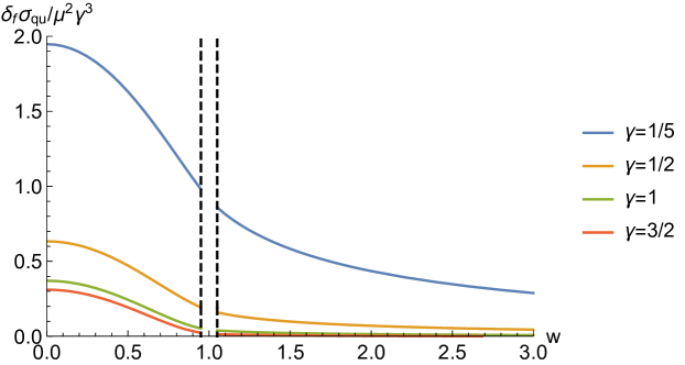
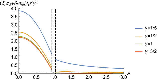
Figure 9: Top: The fermionic quantum one-loop correction $\delta_{f}\sigma_{qu}$ to the domain wall tension. Bottom: The mass renormalization and quantum one-loop correction combined. Note: The dimensionless fermion mass $w$ and Yukawa coupling $\gamma$ are defined in (4.35). Notice that we have divided out by $\mu^{2}\gamma^{3}$. The region near $w=1$ ($m=gv$) is blocked out by dashed lines because the fermions become light and higher derivative corrections become important.

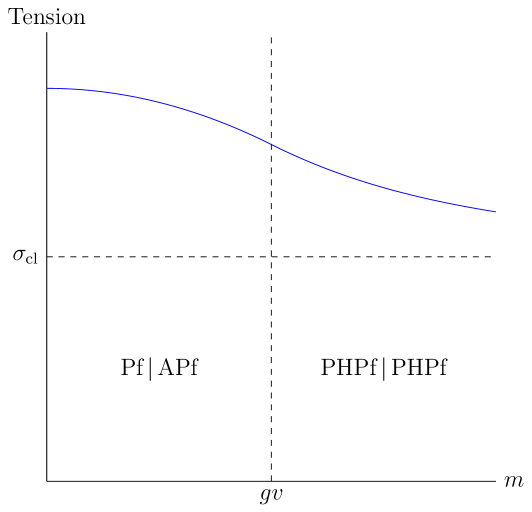
Figure 10: Qualitative dependence of the domain wall tension on the fermion mass $m$, which is a proxy for the disorder strength $\Lambda$. The critical line $m=gv$ separates the Pf/APf and PHPf regimes, and $\sigma_{cl}$ denotes the semi-classical tension in the absence of fermions.

The validity of the lowest order approximation in the derivative expansion was analyzed earlier, and the estimate (4.30) translated to dimensionless quantities becomes

$$|w-1|\gtrsim{{\cal O}(1)\over\gamma}\,.$$ (4.42)

As long as $\gamma$ is ${\cal O}(1)$, the one-loop tension to leading order in the derivative expansion is a valid approximation when $m$ is sufficiently large. Furthermore, if the Yukawa coupling $g$ is large enough relative to $\lambda$, then we can also trust our results in some neighborhood of small $m$. Finally, we have assumed that the couplings $\lambda$ and $g$ are small relative to the masses $w$ and $m$, therefore the higher loop corrections and corrections involving more powers of $\chi$ are suppressed.

4.3.3 The effect of gauging

Let us discuss the effect of the $\mathbb{Z}_{2}$ gauge field on the one-loop tension. Recall that the $\mathbb{Z}_{2}$ gauge field acts as $\Psi^{j}\rightarrow-\Psi^{j}$ and leaves the scalar untouched. In the path integral, having a discrete gauge field amounts to summing over its holonomies. For a domain wall interpolating between two vacua, the Euclidean spacetime is $\mathbb{R}^{3}$ with no boundary or nontrivial cycle, so it is unclear whether the gauging has any effect on the tension at all, even non-perturbatively. On a spacetime with nontrivial cycles, it is logically possible that the sum over holonomies introduces new saddles that dominate over the original saddle (trivial holonomy), but such effects go beyond perturbation theory.

In fact, for the sake of argument, let us imagine that the $\mathbb{Z}_{2}$ is a subgroup of a continuous ${\mathrm{U}}(1)$ gauge symmetry acting on the fermions as $\Psi^{j}\rightarrow\hskip 1.0pt\mathrm{e}^{\hskip 1.0pt\mathrm{i}\hskip 1.0pt\alpha}\Psi^{j}$, with associated gauge connection $A$. In the one-loop effective action from integrating out the fermions, to lowest order in the derivative expansion there in principle is a coupling of the form $(\partial^{\mu}\chi)\,A_{\mu}$. However, we find that the coefficient of this term is zero by an explicit computation in Appendix G.1. Thus the ${\mathrm{U}}(1)$ gauging has no effect at the order of our approximation.

5 Conclusion and future directions

In this work, we have presented an effective field theory that captures the qualitative features of the phase diagram proposed in [15] to describe the $\nu=5/2$ fractional Quantum Hall system. We also studied some simple properties of domain walls present at the time-reversal-symmetric locus (or, in condensed matter terminology, the particle-hole-symmetric locus), including their effective worldvolume theory and their tension, computed to one-loop order in a semiclassical approximation. The tension computed with the EFT is lower in the PH-Pfaffian phase than in the Pfaffian/Anti-Pfaffian phase, suggesting that the former phase may in fact be energetically favored over the latter in the presence of domain walls. This may explain the percolation transition, and serve as a resolution of the dilemma between the experiment [10] (favoring PH-Pfaffian) and bulk energetics studies [18, 19, 20, 21, 22, 23, 24, 25, 26, 27] (favoring Pfaffian/Anti-Pfaffian). We leave a more exhaustive and complete study of bulk/domain wall energetics to future work.

We make some additional remarks related to the bulk and domain wall systems:

1. Pf$\mid$APf domain wall vs PHPf$\mid$PHPf domain wall:
   The Pf$\mid$APf domain wall is well-defined when particle-hole (PH) symmetry is broken, with two different vacua on two sides of bulk. But what do we mean by PHPf$\mid$PHPf domain wall since PHPf presumably has a PH-symmetry preserving bulk? An answer is that in our EFT, the two vacua of the Higgs potential shown in Fig. 5 indeed both break the PH symmetry:

   • The left side of Fig. 5 gives vacua of the PH-symmetry breaking phases Pf and APf.

   • The right side of Fig. 5 gives two vacua both in the PHPf phase, but the two PHPf vacua are exchanged by PH-symmetry. We could have alternatively considered the Higgs potential with the sign of the $\phi^{2}$ term flipped when we are in the PHPf phase — if so, we would have a single PH-symmetry preserving vacuum. But to impose that the $\phi^{2}$ term flips sign around the energy scale $m=gv$ would require a less natural fine-tuning on our EFT. However, the fine tuning could potentially be avoided in the following way. Consider the region near $m=gv$, where the $\phi^{2}$ term sign does not flip “by hand”, but rather the sign flip is induced by the following mechanism. The PH-symmetry breaking Pf$\mid$APf domain wall can transition to the PH-symmetry breaking PHPf$\mid$PHPf domain wall, but the $1+1d$ PHPf$\mid$PHPf domain wall percolation may then induce a $2+1d$ bulk transition to the PHPf phase, which would restore the PH-symmetry dynamically. We propose that this mechanism indeed occurs, while our proposal requires future study.

2. We contrast the order of quantum phase transitions from two perspectives, (i) the domain wall percolating picture [15] versus (ii) our EFT:
   $\bullet$ At zero disorder $\Lambda=0$, both (i) and (ii) have a first order discontinuous phase transition due to PH (or $CT$) breaking and the discontinuity jump at domain wall.
   $\bullet$ At nonzero but small disorder at $\Lambda<\Lambda_{1}$ along the vertical axis $\nu=\nu_{c}$, the case (ii) gives a first order transition, while the case (i) can have a second order transition, or a first order transition effected by disorder broadening the phase boundary (which can result in a new second order transition within the broadening region).
   $\bullet$ Away from the axis $\nu\simeq\nu_{c}$ but within topological orders in the phase diagram Fig. 3, we have second order or continuous transitions derived in our EFT for the case (ii) due to the continuous deformation of mass sign flipping. In the case (i), the percolation phase transition can be indeed a second order transition, at least in the free fermion limit — chiral fermions running on the percolation domain walls where the length scale of puddle diverges at the transition.
   $\bullet$ The upper phase boundary $\Lambda>\Lambda_{2}$ from the topological orders to the thermal metal is also a second order or continuous transition, for both cases (i) and (ii). Physically this transition is similar to an insulator-metal transition driven by strong disorder known as Anderson localization-delocalization transition, which is a second order continuous transition.

3. Our EFT should encode the universality class of gapless topological quantum phase transitions. In our case, we have a second-order continuous phase transition controlled by a free CFT given by 2+1d Dirac or Majorana fermions whose masses flip sign. Naively, the O(2) gauge sector does not directly affect the dynamics and universality class. It will be important to explore further the nature of the phase transitions.

4. We may contrast the emergent global symmetries on the $1+1d$ domain wall (from lower to higher disorder: ${\mathrm{O}}(4)\to{\mathrm{O}}(2)\times{\mathrm{O}}(2)\to\mathbb{Z}_{2}^{F}$ [15]) with the $2+1d$ bulk global symmetries of our $2+1d$ EFT (from lower to higher disorder: $\frac{{\mathrm{O}}(4)}{\mathbb{Z}_{2}}\to\frac{{\mathrm{O}}(2)\times{\mathrm{O}}(2)}{\mathbb{Z}_{2}}\to\mathbb{Z}_{2}^{F}$). The two global symmetry patterns are almost equivalent, but differ by finite group sectors. It turns out that we can also formulate an alternative EFT (by modifying the deformation parameters of the original QFT) to exactly match the bulk and domain wall global symmetry patterns. This will be left for further exploration.

5. Our EFT can choose either two versions PH-Pfaffian_±, depending on how $(CT)^{2}$ assigns to the anyons (they are the same topological order, but different symmetry-enriched topological orders). PH-Pfaffian_+/- have different anomaly, with an anomaly index $\upnu=0$ or $8\in\mathbb{Z}_{16}$, of $CT$ symmetry. If the $\nu=5/2$ system in the lab has PH-Pfaffian_+/- order, then we have less/more IR constraints from the $\upnu=0$ or $8$ anomaly. Moreover, other than this pure $CT$-anomaly, there is also a $CT$-PO(4) mixed anomaly. The ’t Hooft anomaly implies that the associated global symmetry (such as $CT$) is not strictly local and onsite, but it is an emergent global symmetry at low energy and long distances.

We conclude with an incomplete list of additional questions and future directions raised by this study. Of course, most interesting is whether the proposal of [15] indeed provides the correct microscopic description of the $\nu=5/2$ state. If so, we hope our EFT provides a useful conceptual framework for studying aspects of this system.

1. Our effective field theory is a standard relativistic QFT, though various non-relativistic EFTs have been proposed to study quantum Hall systems (see e.g. [6, 7]). Is there a useful non-relativistic bulk EFT description of this system?

   It is worthwhile to note that our EFT is a (super-)renormalizable QFT in $2+1d$, and it is UV complete by itself. Although our EFT does not require a further UV completion at higher energy, it may still be helpful to understand how this relativistic EFT can be obtained from RG flow from a non-relativistic EFT, the electron wavefunctions, or a lattice model at the condensed matter UV cutoff scale.

2. We computed the tension of the domain walls in an approximation where $\lambda/\mu<<1$. Roughly speaking, $\lambda$ and $\mu$ respectively govern the height and width of the domain walls, so that the limit corresponds to studying rigid and thick walls. It would be interesting to determine if the domain walls, assuming they are indeed realized in the $\nu=5/2$ system, actually satisfy this limit so that our tension result can be used reliably to understand energetics of the system.

3. It may be that the particle-hole symmetry is explicitly, weakly broken in the experimental setup. If so, the domain walls would be metastable. It would be instructive to compute the decay rate for these walls in our EFT when one turns on our small but non-vanishing $m_{odd}$ deformation.

4. It would be very instructive to compute the spin-structure-dependent ground state degeneracy by performing an explicit path integral in our EFT. Such a quantity could potentially be measured in a real experimental setting if one fixes the boundary conditions of the lab sample, i.e. periodic or anti-periodic boundary conditions, similar to those on a spatial 2-torus.

6 Acknowledgements

The authors are listed in the alphabetical order by a standard convention. We thank Bert Halperin for a conversation, and Nathan Seiberg and Xiao-Gang Wen for comments on the manuscript. JW thanks Biao Lian for a previous collaboration on [15] and especially acknowledges helpful comments from Jie Wang, Yizhuang You, and Yunqin Zheng. JW also thanks e-mail correspondences from David Mross and Chong Wang, and the feedback from the seminar attendees [65]. YL and NP are each supported by a Sherman Fairchild Postdoctoral Fellowship. JW was supported by NSF Grant PHY-1606531 and Institute for Advanced Study. This work is also supported by NSF Grant DMS-1607871 “Analysis, Geometry and Mathematical Physics” and Center for Mathematical Sciences and Applications at Harvard University. This material is based upon work supported by the U.S. Department of Energy, Office of Science, Office of High Energy Physics, under Award Number DE- SC0011632, and by the Simons Foundation through the Simons Investigator Award.

Appendix A Gravitational Chern-Simons term and thermal Hall response

Any 3-manifold has a spin connection $\omega$. The fermion spinor field of spin $1/2$ couples to the spin connection as $\nabla=\partial-\frac{1}{2}\omega$. Integrating out one massive Majorana fermion $\psi$ gives the gravitational spin Chern-Simons term for positive mass $m$ compared to negative mass:

$$\frac{Z_{\psi,m\gg 0}}{Z_{\psi,m\ll 0}}=\exp\left(\hskip 1.0pt\mathrm{i}\hskip 1.0pt\int_{M_{3}}\text{CS}_{\text{grav}}{\hskip 1.0pt\mathrm{d}^{3}x}\right)~{}.$$ (A.2)

More explicitly,

$$\text{CS}_{\text{grav}}{\hskip 1.0pt\mathrm{d}^{3}x}=\frac{1}{192\pi}\text{Tr }\left(\omega d\omega+\frac{2}{3}\omega^{3}\right)~{}.$$ (A.3)

The spin gravitational Chern-Simons term contributes to the thermal Hall conductivity by a chiral central charge $c_{-}=-1/2$.

Appendix B $\mathbb{Z}_{2}$ gauge theory in $2+1d$

Fermionic SPT phases with an internal unitary $\mathbb{Z}_{2}$ symmetry are known to be classified by $\Omega^{\text{spin}}_{3}=\mathbb{Z}_{8}$. Denote the background $\mathbb{Z}_{2}$ gauge field by $B\in H^{1}(M,\mathbb{Z}_{2})$ for the spacetime $M$. Then the partition function for the $\mathbb{Z}_{2}$ SPT phases can be described using the invertible fermionic TQFT ${\mathrm{SO}}(L)_{1}$ with a special orthogonal ${\mathrm{SO}}(L)$ gauge group as follows:

$$\hskip 1.0pt\mathrm{e}^{\hskip 1.0pt\mathrm{i}\hskip 1.0ptf_{L}(B)}=\left(Z_{{\mathrm{SO}}(L)_{1}}[B]\right)^{*}Z_{{\mathrm{SO}}(L)_{1}}~{},$$ (B.1)

where $Z_{{\mathrm{SO}}(L)_{1}}[B]$ denotes the partition function of ${\mathrm{SO}}(L)_{1}$ coupled to $B$ by the magnetic symmetry $\pi\int w_{2}({\mathrm{SO}}(L))\cup B$, while $\left(Z_{{\mathrm{SO}}(L)_{1}}[B]\right)^{*}$ is its complex conjugate. Since ${\mathrm{SO}}(L)_{1}$ is an invertible spin TQFT, the right hand side is a phase that depends on $B$, which gives the SPT phase $f_{L}(B)$ on the left hand side. By the property ${\mathrm{SO}}(L)_{1}\times{\mathrm{SO}}(L^{\prime})_{1}\leftrightarrow{\mathrm{SO}}(L+L^{\prime})_{1}$, the phase can be written as

$$f_{L}(B)=L\,f(B)~{}$$ (B.2)

for some $f(B)$.

For an even $L$, we can use the property ${\mathrm{SO}}(2)_{1}={\mathrm{U}}(1)_{1}$ to express $Lf(B)=(L/2)\cdot 2f(B)$ as the ${\mathrm{U}}(1)\times{\mathrm{U}}(1)$ Chern-Simons term $-\frac{L/2}{4\pi}B\hskip 1.0pt\mathrm{d}B+\frac{2}{2\pi}B\hskip 1.0pt\mathrm{d}u$ with $u$ constrains $B$ to be a $\mathbb{Z}_{2}$ gauge field. By the field redefinition $u\rightarrow u+B$, we find that for $L=8$ the SPT phase is the same as $L=0$. This reproduces the $\mathbb{Z}_{8}$ classification of the SPT phases

$$L\sim L+8~{}.$$ (B.3)

Gauging the $\mathbb{Z}_{2}$ symmetry with a dynamical gauge field by summing over $B$ gives rise to 8 different $\mathbb{Z}_{2}$ gauge theories. For $L=0$ it is the untwisted $\mathbb{Z}_{2}$ gauge theory (the $\mathbb{Z}_{2}$ toric code), while for $L=4$ it is the Dijkgraaf-Witten twisted $\mathbb{Z}_{2}$ gauge theory (the so-called double semion theory). See the list of 8 different $\mathbb{Z}_{2}$ gauge theories (where $L\in$ even yields an abelian TQFT and $L\in$ odd yields a non-abelian TQFT) in Table 2 of [48].

Appendix C Fermion path integral and counterterms

Consider a $2+1d$ Majorana fermion coupled to a $\mathbb{Z}_{2}$ gauge field $B\in H^{1}(M,\mathbb{Z}_{2})$, and give it a large mass. The fermion path integral depends on the sign of the mass, given by

$$Z[B]_{m>0}=|Z|\exp\left(\frac{\pi\hskip 1.0pt\mathrm{i}\hskip 1.0pt}{2}\eta(B)\right),\quad Z[B]_{m<0}=1~{}.$$ (C.1)

The Atiyah-Patodi-Singer (APS) index theorem relates the exponential of the eta invariant to the topological actions

$$\exp\left(\frac{\pi\hskip 1.0pt\mathrm{i}\hskip 1.0pt}{2}\eta(B)\right)=\exp\left(\hskip 1.0pt\mathrm{i}\hskip 1.0ptf(B)+\hskip 1.0pt\mathrm{i}\hskip 1.0pt\int\text{CS}_{\text{grav}}{\hskip 1.0pt\mathrm{d}^{3}x}\right)~{},$$ (C.2)

where $f(B)$ is the basic fermionic $\mathbb{Z}_{2}$ SPT phase with a $\mathbb{Z}_{2}$ background $B$, and $\int_{\partial Y}\text{CS}_{\text{grav}}{\hskip 1.0pt\mathrm{d}^{3}x}=\frac{1}{192\pi}\int_{Y}\text{Tr}(R\wedge R)$ is the gravitational Chern-Simons term. There are 8 fermionic SPT phases with $\mathbb{Z}_{2}$ symmetry $8f[B]\sim 0$ mod $2\pi$, and they correspond to the 8 pure $\mathbb{Z}_{2}$ gauge theories in $2+1d$ (some of them need a spin structure). We will call them the 8 levels of $2+1d$ $\mathbb{Z}_{2}$ gauge theories; see Appendix B. In our convention, the ${\mathrm{U}}(1)_{4}\times{\mathrm{U}}(1)_{-1}$ theory corresponds to the $6$th class.

The ${\mathrm{O}}(2)$ Chern-Simons gauge theory has two levels: ${\mathrm{O}}(2)_{K,L}$ with the level $K\in\mathbb{Z}$ associated with the instanton number in $4d$, while $L$ represents $8$ $\mathbb{Z}_{2}$ gauge theories $Lf(w_{1}^{{\mathrm{O}}(2)})$, where $w_{1}^{{\mathrm{O}}(2)}$ is the $\mathbb{Z}_{2}$-valued first Stiefel Whitney class of the ${\mathrm{O}}(2)$ bundle.

For massless Majorana fermions in the one-dimensional representation odd under $\mathbb{Z}_{2}$ charge conjugation, we will write the theory using the effective Chern-Simons levels

$${\mathrm{O}}(2)_{K,L}\;\text{CS}+N_{f}\psi\text{ in }\mathbf{1}_{\text{odd}}+M\text{CS}_{\text{grav}}~{},$$ (C.3)

where $M,L$ are integers if $N_{f}$ is even, and half-integers if $N_{f}$ is odd. Integrating out a massive $2+1d$ Majorana fermion shifts the effective Chern-Simons level to be

$$m>0:\;{\mathrm{O}}(2)_{K,L+\frac{1}{2}}\;\text{CS}+(M+\frac{1}{2})\text{CS}_{\text{grav}},\qquad m<0:\;{\mathrm{O}}(2)_{K,L-\frac{1}{2}}\;\text{CS}+(M-\frac{1}{2})\text{CS}_{\text{grav}}~{}.$$ (C.4)

The difference between the shifts for different signs is given by (C.1) and (C.2).

Appendix D Gauging one-form symmetry in $2+1d$ TQFT

Here we review some rules for gauging a one-form symmetry in 2+1$d$ TQFT. For gauging a $\mathbb{Z}_{2}$ one-form symmetry generated by the symmetry generator charge line $a$ of integer spin, the rules are (see e.g. [66, 67, 68, 45]):

• Discard the lines that transform non-trivially under the one-form symmetry. These are the lines (of objects charged under the one-form symmetry) that braid non-trivially with $a$.

• Identify every remaining line $W$ with its fusion with $a$: $W\sim W\cdot a$.

• For the remaining lines that are fixed points under fusion with $a$, there are two copies of the line.

In the corresponding chiral algebra, the procedure is equivalent to extending the chiral algebra by a simple current that obeys, together with the identity, the $\mathbb{Z}_{2}$ fusion algebra.

For instance, ${\mathrm{U}}(1)_{8k}$ Chern-Simons theory has a $\mathbb{Z}_{2}$ subgroup one-form symmetry generated by the Wilson line of charge $4k$ with integer spin. The above procedure produces ${\mathrm{U}}(1)_{2k}$ Chern-Simons theory after gauging one-form $\mathbb{Z}_{2}$ symmetry. Another way to obtain the result is that gauging the one-form symmetry makes the original ${\mathrm{U}}(1)$ gauge field $b$ no longer well-defined, but $b^{\prime}=2b$ is a well-define ${\mathrm{U}}(1)$ gauge field. Expressing the original Chern-Simons term $\frac{8k}{4\pi}b\hskip 1.0pt\mathrm{d}b$ in terms of the ${\mathrm{U}}(1)$ gauge field $b^{\prime}$ gives ${\mathrm{U}}(1)_{2k}$.

Appendix E O(2)_2,L Chern-Simons theories

In this Appendix, we summarize the $2+1d$ O(2)_2,L gauge theories, which are fermionic spin Chern-Simons theories definable on spin manifolds. For the zero level of $2+1d$ $\mathbb{Z}_{2}$ gauge theories (written in terms of ${\mathrm{O}}(2)_{K,L}$ gauge theories with $L\in\mathbb{Z}_{8}$ levels in the previous Appendix), the ${\mathrm{O}}(2)_{2,0}$ gauge theory has the same chiral algebra as the ${\mathrm{U}}(1)_{8}$ gauge theory, and thus we have

$${\mathrm{O}}(2)_{2,0}\;\text{CS}\leftrightarrow{\mathrm{U}}(1)_{8}\;\text{CS}~{}.$$ (E.1)

In general, we denote the $L$th $\mathbb{Z}_{2}$ gauge theory by $T_{L}$ (with an action $Lf[B]$ for the $\mathbb{Z}_{2}$ gauge field $B$), and have the equivalence

$${\mathrm{O}}(2)_{2,L}\;\text{CS}\leftrightarrow\frac{{\mathrm{U}}(1)_{8}\times T_{L}}{\mathbb{Z}_{2}}\;\text{CS}~{},$$ (E.2)

where the quotient denotes gauging a diagonal $\mathbb{Z}_{2}$ one-form symmetry generated by the composite line of the tensor product of the charge 4 Wilson line in ${\mathrm{U}}(1)_{8}$ and the non-transparent fermion line in $T_{L}$ (if we express $T_{L}\leftrightarrow{\mathrm{Spin}}(L)_{-1}\times{\mathrm{SO}}(L)_{1}$, it is the Wilson line in the vector representation of ${\mathrm{Spin}}(L)$).

To compare our present work to Ref.[15], we note that Ref.[15] writes the TQFTs for Pfaffian, PH-Pfaffian, and anti-Pfaffian states as:

Pfaffian $$: \quad\frac{{\mathrm{U}}(1)_{8}\times{{\text{Ising}}}}{\mathbb{Z}_{2}}-4\text{CS}_{\text{grav}},~{}\quad\;\;c_{-}=1+1/2+4/2=7/2.$$ (E.19)

PH-Pfaffian $$: \quad\frac{{\mathrm{U}}(1)_{8}\times{\overline{\text{Ising}}}}{\mathbb{Z}_{2}}-4\text{CS}_{\text{grav}},~{}\quad\;\;c_{-}=1-1/2+4/2=5/2.$$ (E.20)

anti-Pfaffian $$: \quad\frac{{\mathrm{U}}(1)_{8}\times{{\mathrm{SU}}(2)_{-2}}}{\mathbb{Z}_{2}}-4\text{CS}_{\text{grav}},~{}\;c_{-}=1-3/2+4/2=3/2.$$ (E.21)

whereas here we write

Pfaffian $$: \quad{\mathrm{O}}(2)_{2,-1}\;\text{CS}-5\text{CS}_{\text{grav}},~{}\quad c_{-}=1+5/2=7/2.$$ (E.22)

PH-Pfaffian $$: \quad{\mathrm{O}}(2)_{2,1}\;\text{CS}-3\text{CS}_{\text{grav}},~{}\quad\;\;c_{-}=1+3/2=5/2.$$ (E.23)

anti-Pfaffian $$: \quad{\mathrm{O}}(2)_{2,3}\;\text{CS}-\text{CS}_{\text{grav}},~{}\quad\quad\,c_{-}=1+1/2=3/2.$$ (E.24)

In $T_{L}$, the $\mathbb{Z}_{2,[1]}$ symmetry acts on the magnetically charged line, which is the line operator associated to the so-called $\sigma$ anyon. In the condensed matter terminology, this is called the magnetic vortex line or vison loop. $\mathbb{Z}_{2,[1]}$ takes this line to minus itself ($-\sigma$). In the ${\mathrm{U}}(1)_{8}$ Chern-Simons theory, the $\mathbb{Z}_{2,[1]}$ symmetry also transforms the lines with odd ${\mathrm{U}}(1)$ charges to minus themselves. In other words, the line operators of the $\sigma$ anyon in $T_{L}$ and of odd ${\mathrm{U}}(1)$ charge in ${\mathrm{U}}(1)_{8}$ are both charged objects under the diagonal $\mathbb{Z}_{2,[1]}$ 1-form symmetry. As already mentioned in the main text, the $\mathbb{Z}_{2,[1]}$ symmetry generators are line operators in the ${\mathrm{U}}(1)_{8}$ theory with ${\mathrm{U}}(1)$ charge 4 and the fermionic line $f$ in $T_{L}$.

Another way to think of the $\mathbb{Z}_{2,[1]}$ symmetry transformation is that it arises when the charged lines are linked with the symmetry generator lines. Then, the path integral picks up an extra $(-1)$ sign. The link configurations resulting in this sign are

• In the ${\mathrm{U}}(1)_{8}$ Chern-Simons theory, when the odd ${\mathrm{U}}(1)$ charge line links with the ${\mathrm{U}}(1)$ charge 4 line, we get a statistical Berry phase $\exp(\frac{2\pi\hskip 1.0pt\mathrm{i}\hskip 1.0pt}{8}\mathbb{Z}_{odd}\cdot 4)=(-1)$.

• In the $T_{L}$ theory, when the $\sigma$ line links with the the fermionic $f$ line, we get a statistical Berry phase $(-1)$.

We reviewed in Appendix D what it means to gauge a $\mathbb{Z}_{2,[1]}$ symmetry. By gauging the diagonal $\mathbb{Z}_{2,[1]}$ symmetry described above, we reduce the 24 line operators in the ${{\mathrm{U}}(1)_{8}\times T_{L}}$ theory to the 12 line operators in the $\frac{{\mathrm{U}}(1)_{8}\times T_{L}}{\mathbb{Z}_{2}}$ theory. See Tables 1, 2 and 3.

E.1 Hall conductivity

The theory also has a $\mathbb{Z}_{4}$ one-form global symmetry generated by the line with ${\mathrm{U}}(1)$ charge 2 in the ${\mathrm{U}}(1)_{8}$ Chern-Simons theory. One can use this one-form symmetry to couple to a background electromagnetic ${\mathrm{U}}(1)$ gauge field $A$ at level-1 as $\frac{1}{2\pi}(2b)\hskip 1.0pt\mathrm{d}A=\frac{2b}{2\pi}\hskip 1.0pt\mathrm{d}A$. The $U(1)_{8}$ action, including the coupling to the probe electromagnetic background, is:

$$\frac{8}{4\pi}b\hskip 1.0pt\mathrm{d}b+\frac{2b}{2\pi}\hskip 1.0pt\mathrm{d}A~{},$$ (E.25)

where $b$ is the gauge field of ${\mathrm{U}}(1)_{8}$ Chern-Simons theory, and $A$ couples to the properly quantized ${\mathrm{U}}(1)$ gauge field $2b$. This system gives the Hall conductance

$$\sigma_{xy}=2^{2}/8=1/2.$$

In addition, we can add a Chern-Simons action for the background gauge field $A$

$$\int_{3d}\Big{(}\frac{8}{4\pi}b\hskip 1.0pt\mathrm{d}b+\frac{2b}{2\pi}\hskip 1.0pt\mathrm{d}A\Big{)}+\frac{r}{4\pi}A\hskip 1.0pt\mathrm{d}A~{},$$ (E.26)

where the coefficient $r\in\mathbb{Z}$ is quantized to be an integer in fermionic systems. Then the system has a quantum Hall conductance

$$\sigma_{xy}=\frac{1}{2}+r.$$ (E.27)

measured in units of $e^{2}/h$. In the application to the experiment with quantum Hall conductivity $\sigma_{xy}={5\over 2}$ (see [15] and the references therein), we take

$$r=2.$$

Here the $r=2$ corresponds to the lowest (zeroth) Landau levels with both spin-up and spin-down complex fermions, which contribute $\sigma_{xy}=2$ quantum Hall conductance. The first Landau level contributes another $\sigma_{xy}=\frac{1}{2}$ from the half-filled first Landau level with spin-polarized fermions.

The discussion does not change when there are fermions in the nontrivial one-dimensional representation of $\mathbb{Z}_{2}$ (i.e. they are coupled to $T_{L}$ but not ${\mathrm{U}}(1)_{8}$) that do not couple to the background $A$.

There is another way to see the quantum Hall conductance using the $\mathbb{Z}_{4}$ one-form symmetry. The line generating that symmetry has spin $1/4$, and thus the one-form symmetry has the anomaly

$$\frac{8}{4\pi}\int_{4d}B_{2}B_{2}$$ (E.28)

where $B_{2}$ is the two-form background field of the $\mathbb{Z}_{4}$ one-form symmetry. The anomaly then implies that the coupling to $A$ by fixing the value $B_{2}=\frac{1}{4}\hskip 1.0pt\mathrm{d}A$ has a half-integer Hall conductance (see Appendix E of [73]). The one-form symmetry is present in massive or massless theories with the same ’t Hooft anomaly, since the one-form symmetry is preserved by mass deformations, and thus the quantum Hall conductance is the same across the phase diagram.

E.2 Quantum numbers of quasi-excitations

Using (E.2) and (E.26), we see that a line with odd charge in the ${\mathrm{U}}(1)_{8}$ theory is identified with the $\sigma$ line in $T_{L}$ theory. It is therefore the line operator of a non-abelian anyon (when $L$ is odd) with quantum dimension 2. Let us label this line operator as

$$(\text{odd},\sigma).$$

Moreover, we can determine the U(1) electromagnetic charge of this anyonic quasi-excitation from the level $K=8$ and the charge vector ${q}=2$ in (E.26) via

$$Q_{(\text{odd},\sigma)}=\frac{1}{K}{q}=\frac{1}{8}2=\frac{1}{4}.$$

This means our theory has fractional ${\mathrm{U}}(1)$ electromagnetic charges $\pm\frac{1}{4}$ from quasiparticle ${(\text{odd},\sigma)}$ and quasihole excitations.

Two such non-abelian anyons ${(\text{odd},\sigma)}$ fuse to abelian anyons, also called semions, with quantum dimension 1:

$$(\text{even},s).$$

The semions have fractional spin statistics with spin $\frac{1}{4}$, and also have fractional electromagnetic charges:

$$Q_{(\text{even},{s})}=\frac{1}{K}q=\frac{1}{8}2\cdot 2=\frac{1}{2}.$$

Therefore, there are fractional ${\mathrm{U}}(1)$ electromagnetic charges in the theory $\pm\frac{1}{2}$ from the quasiparticle semion ${(\text{even},s)}$ and the corresponding quasihole.

Appendix F Many-body wavefunctions

In this Appendix, we recall and examine the electron wavefunctions for the non-abelian Pf/PHPf/APf states and also abelian states. In contrast to the EFT language used in the bulk of our work (which uses the second-quantization language), this section is formulated in a many-body quantum mechanics picture (the first quantization language). This Appendix can be a companion to the Sec. 3.

F.1 Pfaffian state for $\kappa_{xy}=7/2$

The Pfaffian state wavefunction $\Psi_{\text{Pf}}$ was introduced by Moore-Read [2, 74] for a $\nu=1/2$ fractional quantum Hall state in the zeroth Landau level. It is a rotationally invariant state. The wavefunction is

$$\Psi_{\text{Pf}}(\{z_{i}\})={\rm{Pf}}\left(\frac{1}{z_{i}-z_{j}}\right)\big{(}\prod_{1=i<j}^{N}(z_{i}-z_{j})^{k}\big{)}\hskip 1.0pt\mathrm{e}^{-\sum_{i=1}^{N}|z_{i}|^{2}/4\ell_{B}^{2}}\ .$$ (F.1)

In particular, we look at $k=2$, for $N$ electrons, and for a magnetic length $\ell_{B}=\sqrt{\hbar c/(|e|B)}$ for magnetic field $B$. Here $z_{i}^{*}\equiv\overline{z_{i}}$ is the complex conjugate of the coordinate ${z_{i}}=x_{i}+\hskip 1.0pt\mathrm{i}\hskip 1.0pty_{i}\in\mathbb{C}$. The Pf is the Pfaffian of the rank-$N$ antisymmetric matrix $M_{ij}=1/(z_{i}-z_{j})$, so $({\rm Pf}(M_{ij}))^{2}=\det(M_{ij})$. Namely, for an even positive $N$, we have a degree-$N/2$ polynomial

$${\rm Pf}(M_{ij})={1\over 2^{N/2}(N/2)!}\sum_{\sigma\in S_{N}}{\rm sgn}\sigma\prod_{l=1}^{N/2}M_{\sigma(2l-1)\sigma(2l)},$$

with the symmetry group $S_{N}$ and ${\rm sgn}\sigma=\pm 1$ the signature of the element $\sigma\in S_{N}$, so

$${\rm Pf}(\frac{1}{z_{i}-z_{j}})={1\over 2^{N/2}(N/2)!}\sum_{\sigma\in S_{N}}{\rm sgn}\sigma\prod_{l=1}^{N/2}\frac{1}{z_{\sigma(2l-1)}-z_{\sigma(2l)}}.$$

The ${\rm{Pf}}\left(\frac{1}{z_{i}-z_{j}}\right)$ factor is crucial to obtain an antisymmetric wavefunction, as appropriate for a fermionic electron system. The Laughlin-like factor $\big{(}\prod_{1=i<j}^{N}(z_{i}-z_{j})^{2}\big{)}$ with second-order zeros dictates that there are repulsive interactions between electrons. The ${\rm{Pf}}\left(\frac{1}{z_{i}-z_{j}}\right)$ factor cancels some of the zeros present in the Laughlin-like factor $\big{(}\prod_{1=i<j}^{N}(z_{i}-z_{j})^{2}\big{)}e^{-\sum_{i=1}^{N}|z_{i}|^{2}/4\ell_{B}^{2}}$, making the electrons less repulsive on net. This implies that electrons in $\Psi_{\text{Pf}}$ are closer together than those in a purely Laughlin-like state. All the electrons are spin polarized in the $\Psi_{\text{Pf}}$ state.

Filling fraction: To determine the filling fraction $\nu$ of $\Psi_{\text{Pf}}$, we compute the angular momentum operator $L_{z_{i}}=\hbar({z_{i}}\partial_{z_{i}}-{z_{i}^{*}}\partial_{{z_{i}^{*}}})$ acting on the $i$-th electron. The highest power of $z_{i}$ in $\Psi_{\text{Pf}}$ is $z_{i}^{k(N-1)-1}$ where $k(N-1)-1$ is from the Laughlin factor and $-1$ is from the Pf factor. This gives rise to the angular momentum $k\hbar$ for the $i$-th electron, which encircles the larger area of the droplet with a radius $r_{k}=\sqrt{2(k(N-1)-1)}\ell_{B}$ (at the location where the wavefunction density is maximal). Recall $\Phi_{0}=2\pi(\ell_{B})^{2}B=hc/|e|$, so we verify that $\Psi_{\text{Pf}}$ has the

$$\nu=\frac{\text{number of particles}}{\text{{number of flux quanta}}}=\frac{N}{\Phi_{B}/\Phi_{0}}=\frac{N}{(\pi(r_{k})^{2})/(2\pi(\ell_{B})^{2})}\simeq 1/k,\quad\text{as }N\to\infty,$$

(i.e., $\nu=1/2$ and $\sigma_{xy}=1/2$ for $k=2$ for the Moore-Read Pfaffian). To employ this wavefunction to the study of $\nu=5/2$, we employ the Pf state for the first half-filled, spin-polarized Landau level, while we also include spin up and down electrons fully occupying the zeroth Landau levels. This gives a total filling fraction of $\nu=5/2$; also, $\sigma_{xy}=5/2$. The interaction produces an energy gap the order of the Coulomb interaction energy $e^{2}/\ell_{B}$, so this state is incompressible.

Quasi-excitations: We can obtain a quasihole by adding a hole excitation in a complex coordinate $\zeta$,

$$\Psi_{\text{Pf}}^{\text{hole}}(\zeta;\{z_{i}\})\propto\big{(}\prod_{i^{\prime}=1}^{N}(\zeta-z_{i^{\prime}})\big{)}\Psi_{\text{Pf}}(\{z_{i}\})$$ (F.2)

$$={\rm{Pf}}\left(\frac{(\zeta-z_{i})(\zeta-z_{j})+(\zeta-z_{j})(\zeta-z_{i})}{z_{i}-z_{j}}\right)\big{(}\prod_{1=i<j}^{N}(z_{i}-z_{j})^{k}\big{)}\hskip 1.0pt\mathrm{e}^{-\sum_{i=1}^{N}|z_{i}|^{2}/4\ell_{B}^{2}}.$$

We could view the $z_{i}$ as dynamical variables (that should be integrated over to obtain the density), while viewing $\zeta$ as a background, or probe, parameter. Because the additional factor $\big{(}\prod_{i^{\prime}=1}^{N}(\zeta-z_{i^{\prime}})\big{)}$ introduces more zeros into the wavefunction, the system becomes less repulsive, so also less dense — this is a hallmark of a hole excitation. If $\zeta$ is instead a dynamical variable, then the $(\zeta-z_{i^{\prime}})^{k}$ factor introduces an electron at position $\zeta$. For $\zeta$ a background parameter, this has the interpretation of removing an electron at $\zeta$. Putting this together, a $k$-fold factor $(\zeta-z_{i^{\prime}})^{k}$ removes an electron at $\zeta$ and so, given the electron charge $-|e|$, we have produced a quasihole of charge $|e|/k$. The second line in eqn. (F.2) is a rewriting of the first line, by absorbing the quasihole into the Pf factor: ${\rm{Pf}}\left(\frac{(\zeta_{1}-z_{i})(\zeta_{2}-z_{j})+(\zeta_{2}-z_{j})(\zeta_{1}-z_{i})}{z_{i}-z_{j}}\right)|_{\zeta_{1}=\zeta_{2}=\zeta}$ which can be regarded as the quasihole splitting into two further fractional quasiholes at $\zeta_{1}$ and $\zeta_{2}$, each with charge $|e|/(2k)$. For the Moore-Read Pfaffian at $k=2$, we have a quasihole of charge $|e|/2$ which further fractionate to a quasiholes of charge $|e|/4$.

For each quasihole, there is a corresponding quasiparticle excitation with opposite global symmetry quantum numbers, but with the same spin statistics. The quasiparticles/quasiholes may be regarded as vortices/anti-vortices because the phase of the wavefunction winds when a particle winds around the quasiexcitation at $\zeta$. For example, the fractionalized charge $|e|/4$ or $-|e|/4$ excitations are in fact the $\pm\pi$-vortices, which we shall identify as the non-abelian $\sigma$ anyons in our EFT and TQFTs.

Chiral central charge $c_{-}=c_{L}-c_{R}$ (the degrees of freedom of 1+1$d$ left-moving minus right-moving edge modes) can be determined from two parts of the wavefunctions: first, the Laughlin sector $(z_{i}-z_{j})^{k}$ corresponds to U(1)_k CS theory. It has an edge theory which can be described as a complex chiral boson or fermion, which yields $c_{-}=1$. (The readers can find a systematic description of the $1+1d$ edge theory in Ref. [15].) Second, the Pf factor corresponds to the angular momentum $L_{z}=1$ between the composite fermion with a chiral p-wave ($p_{x}+\hskip 1.0pt\mathrm{i}\hskip 1.0ptp_{y}$) pairing [74]. This gives rise to $c_{-}=1/2$ corresponding to an edge theory given by a real-valued chiral Majorana mode. The total $c_{-}$ for the Pfaffian state eqn. (F.1) is $c_{-}=3/2$.

Composite fermion pairing: The above discussion is consistent with the fact that the Ising TQFT contributes $c_{-}=1/2$ in eqn. (3.3), which can be induced from the $(p_{x}+\hskip 1.0pt\mathrm{i}\hskip 1.0ptp_{y})$-wave pairing of composite fermions (CF), with angular momentum $\propto(k_{x}+\hskip 1.0pt\mathrm{i}\hskip 1.0ptk_{y})$ for $L_{z}=1$. In the Dirac composite Fermi liquid (CFL) picture, the Dirac CF gains a $\pi$-Berry phase around the Fermi surface. For Dirac CF, the pairing becomes the $(d_{x}+\hskip 1.0pt\mathrm{i}\hskip 1.0ptd_{y})$-wave pairing $\propto(k_{x}+\hskip 1.0pt\mathrm{i}\hskip 1.0ptk_{y})^{2}$ with $L_{z}=2$.

F.2 Anti-Pfaffian state for $\kappa_{xy}=3/2$

Anti-Pfaffian (APf) state wavefunction: The bulk system for the Pfaffian state does not have a time-reversal ($CT$)/particle-hole symmetry [28], but Ref. [5] considered the eqn. (F.1)’s particle-hole conjugate wavefunction, dictated by the particle-hole transformation [75], and named it the anti-Pfaffian state:

$$\Psi_{\text{APf}}(\{z_{i}\})=\int(\prod_{{i^{\prime}}=1}^{N}\hskip 1.0pt\mathrm{d}\xi_{i^{\prime}}\hskip 1.0pt\mathrm{d}\xi_{i^{\prime}}^{*})\prod_{i,j^{\prime}=1}^{N}(z_{i}-\xi_{j^{\prime}})\cdot\prod_{1=i^{\prime}<j^{\prime}}^{N}(\xi_{i^{\prime}}-\xi_{j^{\prime}})\hskip 1.0pt\mathrm{e}^{-\sum_{j^{\prime}=1}^{N}|\xi_{j^{\prime}}|^{2}/4\ell_{B}^{2}}\cdot\Psi_{\text{Pf}}(\{\xi_{i^{\prime}}^{*}\})\\ \cdot\prod_{1=i<j}^{N}(z_{i}-z_{j})\cdot\hskip 1.0pt\mathrm{e}^{-\sum_{i=1}^{N}|z_{i}|^{2}/4\ell_{B}^{2}}\ .$$ (F.3)

We can break down the $\Psi_{\text{APf}}$ state we are interested in [4, 5] as a combination of two component pieces. The first piece is the $\nu=1/2$ $\Psi_{\text{APf}}$ with respect to the $\nu=1$ IQH state. The second piece can be viewed as a $\nu=1$ integer quantum Hall state (the IQH state with respect to the $\nu=0$ vacuum). The first part is nothing but the particle-hole conjugate of the $\nu=1/2$ $\Psi_{\text{Pf}}$ with respect to the $\nu=0$ vacuum. Indeed, the first line in eqn. (F.3) corresponds to the first line, while the second line in eqn. (F.3) corresponds to the second part. From this description, we see that the filling fraction is $\nu=1/2$ by construction and the contribution to the chiral central charge of APf from the first part is $c_{-}=-3/2$ and from the second part is $c_{-}=1$ for a total of $c_{-}=-3/2+1=-1/2$.

The ${\mathrm{SU}}(2)_{-2}$ TQFT contributes $c_{-}=-3/2$ in eqn. (3.5), which can be induced from the $(f_{x}-\hskip 1.0pt\mathrm{i}\hskip 1.0ptf_{y})$-wave pairing of CF, with its angular momentum $\propto(k_{x}-\hskip 1.0pt\mathrm{i}\hskip 1.0ptk_{y})^{3}$ for $L_{z}=-3$. For Dirac CF, the pairing becomes the $(d_{x}-\hskip 1.0pt\mathrm{i}\hskip 1.0ptd_{y})$-wave pairing with $L_{z}=-2$.

F.3 Particle-Hole Pfaffian state for $\kappa_{xy}=5/2$

Particle-Hole Pfaffian (PH-Pfaffian, or PHPf) wavefunction [9] (see also [76, 77] and other attempts [78, 79]) can be written as

$$\Psi_{\mathrm{PHPf}}(\{z_{i}\})=\mathcal{P}_{\mathrm{LLL}}\left[\mathrm{Pf}\left(\frac{1}{z_{i}^{*}-z_{j}^{*}}\right)\big{(}\prod_{1=i<j}^{N}(z_{i}-z_{j})^{2}\big{)}e^{-\sum_{i=1}^{N}|z_{i}|^{2}/4\ell_{B}^{2}}\right]\\ \simeq\int(\prod_{{i^{\prime}}=1}^{N}\hskip 1.0pt\mathrm{d}\xi_{i^{\prime}}\hskip 1.0pt\mathrm{d}\xi_{i^{\prime}}^{*})\langle\{z_{i}\}|\{\xi_{i^{\prime}}\}\rangle\left[\mathrm{Pf}\left(\frac{1}{\xi_{i^{\prime}}^{*}-\xi_{j^{\prime}}^{*}}\right)\big{(}\prod_{1=i<j}^{N}(\xi_{i^{\prime}}-\xi_{j^{\prime}})^{2}\big{)}\hskip 1.0pt\mathrm{e}^{-\sum_{i^{\prime}=1}^{N}|\xi_{i^{\prime}}|^{2}/4\ell_{B}^{2}}\right]\\ =\int(\prod_{{i^{\prime}}=1}^{N}\hskip 1.0pt\mathrm{d}\xi_{i^{\prime}}\hskip 1.0pt\mathrm{d}\xi_{i^{\prime}}^{*})\exp\big{(}-(|\xi_{i^{\prime}}|^{2}-2{\xi_{i^{\prime}}^{*}}z_{i}+|z_{i}|^{2})/(4l_{B}^{2})\big{)}\\ \cdot\left[\mathrm{Pf}\left(\frac{1}{\xi_{i^{\prime}}^{*}-\xi_{j^{\prime}}^{*}}\right)\big{(}\prod_{1=i<j}^{N}(\xi_{i^{\prime}}-\xi_{j^{\prime}})^{2}\big{)}\hskip 1.0pt\mathrm{e}^{-\sum_{i^{\prime}=1}^{N}|\xi_{i^{\prime}}|^{2}/4\ell_{B}^{2}}\right].$$ (F.4)

The $\mathcal{P}_{\mathrm{LLL}}$ is the projection onto the lowest Landau level (LLL). From the first line in eqn. (F.4), we can see that the filling fraction is still $\nu=1/2$, as one can read off from the Laughlin factor using the same reasoning from the Pfaffian case. Moreover, the $\mathrm{Pf}\left(\frac{1}{z_{i}^{*}-z_{j}^{*}}\right)$ tells us the pairing of composite fermions possesses angular momentum $L_{z}=-1$ between the composite fermion with an anti-chiral p-wave ($p_{x}-\hskip 1.0pt\mathrm{i}\hskip 1.0ptp_{y}$) pairing[74], which gives rise to $c_{-}=1/2$. The total chiral central charge of the PH-Pfaffian eqn. (F.3) therefore has $c_{-}=1-1/2=1/2$. The second line in eqn. (F.4) rewrites the projection in terms of the coherent state projection so the wave function is projected into the LLL.

The above discussion is consistent with the fact that the $\overline{\text{Ising}}$ TQFT contributes $c_{-}=-1/2$ in eqn. (3.4), which can be induced from the $(p_{x}-\hskip 1.0pt\mathrm{i}\hskip 1.0ptp_{y})$-wave pairing of CF, with angular momentum $\propto(k_{x}-\hskip 1.0pt\mathrm{i}\hskip 1.0ptk_{y})$ at $L_{z}=-1$. For a Dirac CF picture, the pairing becomes the $s$-wave pairing with $L_{z}=0$.

F.4 $K=8$-state for $\kappa_{xy}=3$

$K=8$-state wavefunction is a bosonic wavefunction but can be written as a fermionic wavefunction by dressing it with a fermionic tensor product state:

$$\Psi_{{K=8}}(\{z_{i}\}\})=\big{(}\prod_{1=i<j}^{N}(z_{i}-z_{j})^{8}\big{)}\hskip 1.0pt\mathrm{e}^{-\sum_{i=1}^{N}|z_{i}|^{2}/4\ell_{B}^{2}}\cdot(\text{fermionic tensor product state})\ .$$ (F.5)

The filling fraction is $\nu=1/2$ with an appropriate charge coupling, when the charge $2e$ quasi-excitations are coupled to the ${\mathrm{U}}(1)$ electromagnetic gauge field at level-1. The chiral central charge is $c_{-}=1$, as always for a Laughlin wavefunction. The is consistent with ${\mathrm{U}}(1)_{8}$ TQFT with $c_{-}=1$.

F.5 113-state for $\kappa_{xy}=2$

113-state wavefunction is a special case of the lmn wavefunction, known as the Halperin wavefunction (the multi-component generalization of Laughlin wavefunction) with ${\rm l}=1$, ${\rm m}=1$, ${\rm n}=3$ for some $N+N^{\prime}$ electron system:

$$\Psi_{{113}}(\{z_{i}\},\{w_{i^{\prime}}\})=\big{(}\prod_{1=i<j}^{N}(z_{i}-z_{j})^{\rm l}\big{)}\big{(}\prod_{1=i^{\prime}<j^{\prime}}^{N^{\prime}}(w_{i^{\prime}}-w_{j^{\prime}})^{\rm m}\big{)}\big{(}\prod_{i}^{N}\prod_{j^{\prime}}^{N^{\prime}}(z_{i}-w_{j^{\prime}})^{\rm n}\big{)}\\ \left.\hskip 1.0pt\mathrm{e}^{-\sum_{i=1}^{N}|z_{i}|^{2}/4\ell_{B}^{2}}e^{-\sum_{i^{\prime}=1}^{N}|w_{i^{\prime}}|^{2}/4\ell_{B}^{2}}\right|_{{\rm l}=1,\,{\rm m}=1,\,{\rm n}=3}\ .$$ (F.6)

The filling fraction is $\nu=1/2$ with an appropriate charge coupling. The chiral central charge is $c_{-}=1-1=0$ coming from two modes with opposite chiralities.

In general, we expect that quasiparticles and quasiholes of the above many-body wavefunctions in this Appendix agree with the anyons (and their quantum numbers) of TQFTs shown in Table 1, 2, 3, 4, and 5 in Sec. 3.

Appendix G One-loop computations

G.1 Fermionic functional determinant

We explicitly carry out the computation of some terms in the fermionic functional determinant given by integrating out a Dirac fermion $\Psi$ in the following Lagrangian in $d$ spacetime dimensions:

$${\cal L}=\overline{\Psi}(\hskip 1.0pt\mathrm{i}\hskip 1.0pt{\ooalign{\hfil\hfil/\hfil\cr$D$}}+m-{\ooalign{\hfil\hfil/\hfil\cr$A$}}-\chi)\Psi\,.$$ (G.1)

The quadratic term in the functional determinant effective action is formally written as

$${1\over 2}\,{\rm Tr}\,{{\ooalign{\hfil\hfil/\hfil\cr$p$}}-m\over p^{2}+m^{2}}\,(\chi+{\ooalign{\hfil\hfil/\hfil\cr$A$}})\,{{\ooalign{\hfil\hfil/\hfil\cr$p$}}-m\over p^{2}+m^{2}}\,(\chi+{\ooalign{\hfil\hfil/\hfil\cr$A$}})\,.$$ (G.2)

For the $\chi^{2}$ piece, we simplify by

$${1\over 2}\,{\rm Tr}\,{{\ooalign{\hfil\hfil/\hfil\cr$p$}}-m\over p^{2}+m^{2}}\,\chi\,{{\ooalign{\hfil\hfil/\hfil\cr$p$}}-m\over p^{2}+m^{2}}\,\chi$$ (G.3)

$$={1\over 2}\,{\rm Tr}\,{{\ooalign{\hfil\hfil/\hfil\cr$p$}}-m\over p^{2}+m^{2}}\,{{\ooalign{\hfil\hfil/\hfil\cr$p$}}-\hskip 1.0pt\mathrm{i}\hskip 1.0pt{\ooalign{\hfil\hfil/\hfil\cr$\partial$}}-m\over(p-\hskip 1.0pt\mathrm{i}\hskip 1.0pt\partial)^{2}+m^{2}}\,\chi\,\chi$$

$$={1\over 2}\,{\rm Tr}\,{{-p^{2}+m^{2}-2m{\ooalign{\hfil\hfil/\hfil\cr$p$}}+\hskip 1.0pt\mathrm{i}\hskip 1.0pt(p\partial+m{\ooalign{\hfil\hfil/\hfil\cr$\partial$}})}\over{(p^{2}+m^{2})^{2}}}\sum_{n=0}^{\infty}\left({{2\hskip 1.0pt\mathrm{i}\hskip 1.0ptp\partial+\partial^{2}}\over{p^{2}+m^{2}}}\right)^{n}\,\chi\,\chi\,,$$

where the derivatives only act on the first $\chi$ and not the second. The formal expression can be explicitly evaluated by the momentum space integral

$$\int{\hskip 1.0pt\mathrm{d}^{d}p\over(2\pi)^{d}}\,.$$ (G.4)

The trace simply kills all slashed objects. We will compute up to $\partial^{4}$ order, so we keep up to $n=4$ in the sum. By Lorentz invariance, we can perform the following replacements in the integrand:

$$(p\partial)^{2}\to{1\over d}p^{2}\partial^{2}\,,\quad(p\partial)^{4}\to{3\over d(d+2)}p^{4}\partial^{4}$$ (G.5)

The result is

$${1\over 2}\,\chi\left({|m|\over\pi}-{1\over 12\pi|m|}\partial^{2}-{1\over 240\pi|m|^{3}}\,\partial^{4}+{\cal O}(\partial^{6})\right)\chi\,.$$ (G.6)

Next, let us consider the $\chi A$ piece.

$${1\over 2}\,{\rm Tr}\,{{\ooalign{\hfil\hfil/\hfil\cr$p$}}-m\over p^{2}+m^{2}}\,\chi\,{{\ooalign{\hfil\hfil/\hfil\cr$p$}}-m\over p^{2}+m^{2}}\,{\ooalign{\hfil\hfil/\hfil\cr$A$}}$$ (G.7)

$$={1\over 2}\,{\rm Tr}\,{{\ooalign{\hfil\hfil/\hfil\cr$p$}}-m\over p^{2}+m^{2}}\,{{\ooalign{\hfil\hfil/\hfil\cr$p$}}-\hskip 1.0pt\mathrm{i}\hskip 1.0pt{\ooalign{\hfil\hfil/\hfil\cr$\partial$}}-m\over(p-\hskip 1.0pt\mathrm{i}\hskip 1.0pt\partial)^{2}+m^{2}}\,\chi{\ooalign{\hfil\hfil/\hfil\cr$A$}}$$

$$={1\over 2}\,{\rm Tr}\,{-p^{2}+m^{2}-2m{\ooalign{\hfil\hfil/\hfil\cr$p$}}+\hskip 1.0pt\mathrm{i}\hskip 1.0pt(p\partial+m{\ooalign{\hfil\hfil/\hfil\cr$\partial$}})\over(p^{2}+m^{2})^{2}}\sum_{n=0}^{\infty}\left({2\hskip 1.0pt\mathrm{i}\hskip 1.0ptp\partial+\partial^{2}\over p^{2}+m^{2}}\right)^{n}\,\chi{\ooalign{\hfil\hfil/\hfil\cr$A$}}\,,$$

where the derivatives only act on $\chi$ but not $A$. Evaluating the trace gives

$${2^{\lfloor d/2\rfloor}\over 2}\,{2mp^{\mu}-\hskip 1.0pt\mathrm{i}\hskip 1.0ptm\partial^{\mu}\over(p^{2}+m^{2})^{2}}\sum_{n=0}^{\infty}\left({2\hskip 1.0pt\mathrm{i}\hskip 1.0ptp\partial+\partial^{2}\over p^{2}+m^{2}}\right)^{n}\,\chi A_{\mu}\,.$$ (G.8)

The pieces with only one derivative combine to

$${2^{\lfloor d/2\rfloor}\over 2}{\hskip 1.0pt\mathrm{i}\hskip 1.0ptm}\int{\hskip 1.0pt\mathrm{d}^{d}p\over(2\pi)^{d}}{-(p^{2}+m^{2})\delta^{\mu\nu}+4p^{\mu}p^{\nu}\over(p^{2}+m^{2})^{3}}\,(\partial_{\nu}\chi)\,A_{\mu}$$ (G.9)

$$={2^{\lfloor d/2\rfloor}\over 2}{\hskip 1.0pt\mathrm{i}\hskip 1.0ptm}\int{\hskip 1.0pt\mathrm{d}^{d}p\over(2\pi)^{d}}\,{(4/d-1)p^{2}-m^{2}\over(p^{2}+m^{2})^{3}}(\partial^{\mu}\chi)\,A_{\mu}\,,$$

whose coefficient in $d=3$ evaluates to

$${\hskip 1.0pt\mathrm{i}\hskip 1.0ptm\over 2\pi^{2}}\int_{0}^{\infty}\hskip 1.0pt\mathrm{d}p\,p^{2}\,{(p^{2}/3-m^{2})\over(p^{2}+m^{2})^{3}}=0\,.$$ (G.10)

As for the $A\chi$ piece,

$${1\over 2}\,{\rm Tr}\,{{\ooalign{\hfil\hfil/\hfil\cr$p$}}-m\over p^{2}+m^{2}}\,{\ooalign{\hfil\hfil/\hfil\cr$A$}}\,{{\ooalign{\hfil\hfil/\hfil\cr$p$}}-m\over p^{2}+m^{2}}\,\chi$$ (G.11)

$$={1\over 2}\,{\rm Tr}\,{{\ooalign{\hfil\hfil/\hfil\cr$p$}}-m\over p^{2}+m^{2}}\,\gamma^{\mu}\,{{\ooalign{\hfil\hfil/\hfil\cr$p$}}-\hskip 1.0pt\mathrm{i}\hskip 1.0pt{\ooalign{\hfil\hfil/\hfil\cr$\partial$}}-m\over(p-\hskip 1.0pt\mathrm{i}\hskip 1.0pt\partial)^{2}+m^{2}}\,A_{\mu}\chi$$

$$={1\over 2}\,{\rm Tr}\,{({\ooalign{\hfil\hfil/\hfil\cr$p$}}-m)\gamma^{\mu}({\ooalign{\hfil\hfil/\hfil\cr$p$}}-\hskip 1.0pt\mathrm{i}\hskip 1.0pt{\ooalign{\hfil\hfil/\hfil\cr$\partial$}}-m)\over(p^{2}+m^{2})^{2}}\sum_{n=0}^{\infty}\left({2\hskip 1.0pt\mathrm{i}\hskip 1.0ptp\partial+\partial^{2}\over p^{2}+m^{2}}\right)^{n}\,A_{\mu}\chi$$

$$={1\over 2}\,{\rm Tr}\,{-\hskip 1.0pt\mathrm{i}\hskip 1.0pt{\ooalign{\hfil\hfil/\hfil\cr$p$}}\gamma^{\mu}{\ooalign{\hfil\hfil/\hfil\cr$\partial$}}-m\gamma^{\mu}({\ooalign{\hfil\hfil/\hfil\cr$p$}}-\hskip 1.0pt\mathrm{i}\hskip 1.0pt{\ooalign{\hfil\hfil/\hfil\cr$\partial$}})-m{\ooalign{\hfil\hfil/\hfil\cr$p$}}\gamma^{\mu}\over(p^{2}+m^{2})^{2}}\sum_{n=0}^{\infty}\left({2\hskip 1.0pt\mathrm{i}\hskip 1.0ptp\partial+\partial^{2}\over p^{2}+m^{2}}\right)^{n}\,A_{\mu}\chi$$

$$={2^{\lfloor d/2\rfloor}\over 2}\,{\hskip 1.0pt\mathrm{i}\hskip 1.0pt\varepsilon^{\nu\mu\sigma}p_{\nu}\partial_{\sigma}+m(2p^{\mu}-\hskip 1.0pt\mathrm{i}\hskip 1.0pt\partial^{\mu})\over(p^{2}+m^{2})^{2}}\sum_{n=0}^{\infty}\left({2\hskip 1.0pt\mathrm{i}\hskip 1.0ptp\partial+\partial^{2}\over p^{2}+m^{2}}\right)^{n}\,A_{\mu}\chi\,,$$

where the derivatives act on $A$ but not $\chi$, and the parity odd piece with a Levi-Civita symbol is present only if $d=3$. At one derivative order, the parity odd piece vanishes upon integrating over $p$, and we are left with the same expression as the $\chi A$ term (G.8) except now the derivative acts on $A$ instead of $\chi$. Thus, upon integration by parts, the $A\chi$ term is an identical contribution to the effective action as the $\chi A$ term. When $d=3$, the coefficient of $(\partial_{\mu}\chi)\,A^{\mu}$ in the effective Lagrangian vanishes, as we found in (G.10).

G.2 Domain wall tension

Let us discuss how to practically perform the computation of the fermionic one-loop contribution to the domain wall tension, given by the formula (4.39). The log determinant of the first-order differential operator $\mathbb{D}_{m,g}^{\phi=\phi_{0}}$ can be related to those of second-order differential operators. Let $\varepsilon$ be the Levi-Civita symbol. Formally,

$$\log\det\mathbb{D}_{m,g}^{\phi=\phi_{0}}={1\over 2}\log\det(\varepsilon\mathbb{D}_{m,g}^{\phi=\phi_{0}})^{2}\,.$$ (G.12)

Next, we write everything explicitly in transverse momentum space,

$$\log\det\mathbb{D}_{m,g}^{\phi=\phi_{0}}=\int{\hskip 1.0pt\mathrm{d}^{2}k_{\parallel}\over(2\pi)^{2}}\log\det\mathbb{D}_{m,g;k_{\parallel}}^{\phi=\phi_{0}}={1\over 2}\int{\hskip 1.0pt\mathrm{d}^{2}k_{\parallel}\over(2\pi)^{2}}\log\det(\varepsilon\mathbb{D}_{m,g;k_{\parallel}}^{\phi=\phi_{0}})^{2}\,,$$ (G.13)

where

$$\mathbb{D}_{m,g;k_{\parallel}}^{\phi=\phi_{0}}\equiv\begin{pmatrix}\displaystyle-\partial_{z}+m+g\phi_{0}(z)&k_{0}-\hskip 1.0pt\mathrm{i}\hskip 1.0ptk_{2}\\ -k_{0}-\hskip 1.0pt\mathrm{i}\hskip 1.0ptk_{2}&\displaystyle\partial_{z}+m+g\phi_{0}(z)&\end{pmatrix}\,,$$ (G.14)

and

$$(\varepsilon\mathbb{D}_{m,g;k_{\parallel}}^{\phi=\phi_{0}})^{2}=\begin{pmatrix}-\partial_{z}^{2}+(g\phi_{0}(z)-m)^{2}-g\phi^{\prime}_{0}(z)+k_{\parallel}^{2}&0\\ 0&-\partial_{z}^{2}+(g\phi_{0}(z)-m)^{2}+g\phi^{\prime}_{0}(z)+k_{\parallel}^{2}\end{pmatrix}$$ (G.15)

is a diagonal matrix of second order differential operators. If we define

$$\mathbb{M}_{m,g;k_{\parallel}}^{\phi=\phi_{0}}\equiv-\partial_{z}^{2}+(g\phi_{0}(z)-m)^{2}-g\phi^{\prime}_{0}(z)+k_{\parallel}^{2}\,,$$ (G.16)

then

$$\log\det\mathbb{D}_{m,g;k_{\parallel}}^{\phi=\phi_{0}}={1\over 2}(\log\det\mathbb{M}_{m,g;k_{\parallel}}^{\phi=\phi_{0}}+\log\det\mathbb{M}_{-m,-g;k_{\parallel}}^{\phi=\phi_{0}})\,.$$ (G.17)

Hence, the integral (4.39) can written as

$$\delta_{f}\sigma =-{1\over 2}\int{\hskip 1.0pt\mathrm{d}^{2}k_{\parallel}\over(2\pi)^{2}}\Bigg{[}\log{\det\mathbb{M}_{m,g;k_{\parallel}}^{\phi=\phi_{0}}\over\det\mathbb{M}_{m,g;k_{\parallel}}^{\phi=v}}{\det\mathbb{M}_{-m,g;k_{\parallel}}^{\phi=\phi_{0}}\over\det\mathbb{M}_{-m,g;k_{\parallel}}^{\phi=v}}{\det\mathbb{M}_{m,-g;k_{\parallel}}^{\phi=\phi_{0}}\over\det\mathbb{M}_{m,-g;k_{\parallel}}^{\phi=v}}{\det\mathbb{M}_{-m,-g;k_{\parallel}}^{\phi=\phi_{0}}\over\det\mathbb{M}_{-m,-g;k_{\parallel}}^{\phi=v}}$$ (G.18)

$$\hskip 72.26999pt-{Fg(g+m/v)\over(k_{\parallel}^{2}+(gv+m)^{2})^{1/2}}-{Fg(g-m/v)\over(k_{\parallel}^{2}+(gv-m)^{2})^{1/2}}\Bigg{]}\,.$$

To compute the log determinants in the integrand, we apply the Gel’fand-Yaglom theorem to relate $\log\det\mathbb{M}_{m,g;k_{\parallel}}^{\phi}$ to a boundary value problem for the second order differential operator $\mathbb{M}_{m,g;k_{\parallel}}^{\phi}$, and solve it numerically, as in [56].

References

- [1] R. Willett, J. P. Eisenstein, H. L. Störmer, D. C. Tsui, A. C. Gossard, and J. H. English, “Observation of an even-denominator quantum number in the fractional quantum hall effect,” Phys. Rev. Lett. 59 (Oct, 1987) 1776–1779. https://link.aps.org/doi/10.1103/PhysRevLett.59.1776.
- [2] G. Moore and N. Read, “Nonabelions in the fractional quantum hall effect,” Nucl. Phys. B 360 no. 2, (1991) 362 – 396.
- [3] X. G. Wen, “Non-abelian statistics in the fractional quantum hall states,” Phys. Rev. Lett. 66 (Feb, 1991) 802–805. https://link.aps.org/doi/10.1103/PhysRevLett.66.802.
- [4] M. Levin, B. I. Halperin, and B. Rosenow, “Particle-hole symmetry and the pfaffian state,” Phys. Rev. Lett. 99 (Dec, 2007) 236806. https://link.aps.org/doi/10.1103/PhysRevLett.99.236806.
- [5] S.-S. Lee, S. Ryu, C. Nayak, and M. P. A. Fisher, “Particle-hole symmetry and the quantum hall state,” Phys. Rev. Lett. 99 (Dec, 2007) 236807. https://link.aps.org/doi/10.1103/PhysRevLett.99.236807.
- [6] D. T. Son, “Is the composite fermion a dirac particle?,” Phys. Rev. X 5 (Sep, 2015) 031027, arXiv:1502.03446 [cond-mat.mes-hall].
- [7] B. I. Halperin, P. A. Lee, and N. Read, “Theory of the half-filled landau level,” Phys. Rev. B 47 (Mar, 1993) 7312–7343.
- [8] T. Jolicoeur, “Non-abelian states with negative flux: A new series of quantum hall states,” Physical Review Letters 99 no. 3, (Jul, 2007) , arXiv:0705.1619 [cond-mat.mes-hall]. http://dx.doi.org/10.1103/physrevlett.99.036805.
- [9] P. T. Zucker and D. E. Feldman, “Stabilization of the particle-hole pfaffian order by landau-level mixing and impurities that break particle-hole symmetry,” Phys. Rev. Lett. 117 (Aug, 2016) 096802. https://link.aps.org/doi/10.1103/PhysRevLett.117.096802.
- [10] M. Banerjee, M. Heiblum, V. Umansky, D. E. Feldman, Y. Oreg, and A. Stern, “Observation of half-integer thermal Hall conductance,” Nature 559 no. 7713, (2018) 205–210, arXiv:1710.00492 [cond-mat.mes-hall].
- [11] C. L. Kane and M. P. A. Fisher, “Quantized thermal transport in the fractional quantum hall effect,” Phys. Rev. B 55 (Jun, 1997) 15832–15837. https://link.aps.org/doi/10.1103/PhysRevB.55.15832.
- [12] X.-G. Wen, “Topological order and edge structure of =1/2 quantum hall state,” Phys. Rev. Lett. 70 (Jan, 1993) 355–358. https://link.aps.org/doi/10.1103/PhysRevLett.70.355.
- [13] D. F. Mross, Y. Oreg, A. Stern, G. Margalit, and M. Heiblum, “Theory of disorder-induced half-integer thermal hall conductance,” Phys. Rev. Lett. 121 (Jul, 2018) 026801. https://link.aps.org/doi/10.1103/PhysRevLett.121.026801.
- [14] C. Wang, A. Vishwanath, and B. I. Halperin, “Topological order from disorder and the quantized hall thermal metal: Possible applications to the state,” Phys. Rev. B 98 (Jul, 2018) 045112. https://link.aps.org/doi/10.1103/PhysRevB.98.045112.
- [15] B. Lian and J. Wang, “Theory of the disordered quantum thermal Hall state: Emergent symmetry and phase diagram,” Phys. Rev. B97 no. 16, (2018) 165124, arXiv:1801.10149 [cond-mat.mes-hall].
- [16] X. Chen, L. Fidkowski, and A. Vishwanath, “Symmetry enforced non-abelian topological order at the surface of a topological insulator,” Phys. Rev. B 89 (Apr, 2014) 165132. https://link.aps.org/doi/10.1103/PhysRevB.89.165132.
- [17] M. A. Metlitski, L. Fidkowski, X. Chen, and A. Vishwanath, “Interaction effects on 3D topological superconductors: surface topological order from vortex condensation, the 16 fold way and fermionic Kramers doublets,” arXiv:1406.3032 [cond-mat.str-el].
- [18] R. H. Morf, “Transition from quantum hall to compressible states in the second landau level: New light on the enigma,” Phys. Rev. Lett. 80 (Feb, 1998) 1505–1508. https://link.aps.org/doi/10.1103/PhysRevLett.80.1505.
- [19] E. H. Rezayi and F. D. M. Haldane, “Incompressible paired hall state, stripe order, and the composite fermion liquid phase in half-filled landau levels,” Phys. Rev. Lett. 84 (May, 2000) 4685–4688. https://link.aps.org/doi/10.1103/PhysRevLett.84.4685.
- [20] M. R. Peterson, T. Jolicoeur, and S. Das Sarma, “Finite-layer thickness stabilizes the pfaffian state for the 5/2 fractional quantum hall effect: Wave function overlap and topological degeneracy,” Phys. Rev. Lett. 101 (Jul, 2008) 016807. https://link.aps.org/doi/10.1103/PhysRevLett.101.016807.
- [21] A. E. Feiguin, E. Rezayi, K. Yang, C. Nayak, and S. Das Sarma, “Spin polarization of the quantum hall state,” Phys. Rev. B 79 (Mar, 2009) 115322. https://link.aps.org/doi/10.1103/PhysRevB.79.115322.
- [22] H. Wang, D. N. Sheng, and F. D. M. Haldane, “Particle-hole symmetry breaking and the fractional quantum hall effect,” Phys. Rev. B 80 (Dec, 2009) 241311. https://link.aps.org/doi/10.1103/PhysRevB.80.241311.
- [23] M. Storni, R. H. Morf, and S. Das Sarma, “Fractional quantum hall state at and the moore-read pfaffian,” Phys. Rev. Lett. 104 (Feb, 2010) 076803. https://link.aps.org/doi/10.1103/PhysRevLett.104.076803.
- [24] E. H. Rezayi and S. H. Simon, “Breaking of particle-hole symmetry by landau level mixing in the quantized hall state,” Phys. Rev. Lett. 106 (Mar, 2011) 116801. https://link.aps.org/doi/10.1103/PhysRevLett.106.116801.
- [25] Z. Papić, F. D. M. Haldane, and E. H. Rezayi, “Quantum phase transitions and the fractional hall state in wide quantum wells,” Phys. Rev. Lett. 109 (Dec, 2012) 266806. https://link.aps.org/doi/10.1103/PhysRevLett.109.266806.
- [26] M. P. Zaletel, R. S. K. Mong, F. Pollmann, and E. H. Rezayi, “Infinite density matrix renormalization group for multicomponent quantum hall systems,” Phys. Rev. B 91 (Jan, 2015) 045115. https://link.aps.org/doi/10.1103/PhysRevB.91.045115.
- [27] K. Pakrouski, M. R. Peterson, T. Jolicoeur, V. W. Scarola, C. Nayak, and M. Troyer, “Phase diagram of the fractional quantum hall effect: Effects of landau-level mixing and nonzero width,” Phys. Rev. X 5 (Apr, 2015) 021004. https://link.aps.org/doi/10.1103/PhysRevX.5.021004.
- [28] M. Greiter, X.-G. Wen, and F. Wilczek, “Paired Hall state at half filling,” Phys. Rev. Lett. 66 (1991) 3205–3208.
- [29] Y. Imry and S.-k. Ma, “Random-field instability of the ordered state of continuous symmetry,” Phys. Rev. Lett. 35 (Nov, 1975) 1399–1401. https://link.aps.org/doi/10.1103/PhysRevLett.35.1399.
- [30] J. T. Chalker and P. D. Coddington, “Percolation, quantum tunnelling and the integer hall effect,” J. Phys. C 21 no. 14, (1988) 2665.
- [31] S. H. Simon, “Interpretation of thermal conductance of the ?=5/2 edge,” Phys. Rev. B97 no. 12, (2018) 121406, arXiv:1801.09687 [cond-mat.mes-hall].
- [32] K. K. Ma and D. Feldman, “Partial equilibration of integer and fractional edge channels in the thermal quantum Hall effect,” Phys. Rev. B 99 no. 8, (2019) 085309, arXiv:1809.05488 [cond-mat.mes-hall].
- [33] S. H. Simon and B. Rosenow, “Partial equilibration of the anti-pfaffian edge due to majorana disorder,” arXiv:1906.05294 [cond-mat.str-el].
- [34] S. H. Simon, M. Ippoliti, M. P. Zaletel, and E. H. Rezayi, “Energetics of pfaffian?anti-pfaffian domains,” Physical Review B 101 no. 4, (Jan, 2020) , arXiv:1909.12844 [cond-mat.mes-hall]. http://dx.doi.org/10.1103/physrevb.101.041302.
- [35] H. Asasi and M. Mulligan, “Partial equilibration of anti-pfaffian edge modes at ,” arXiv:2004.04161 [cond-mat.str-el].
- [36] D. E. Feldman, “Comment on ?Interpretation of thermal conductance of the ?=5/2 edge?,” Phys. Rev. B98 no. 16, (2018) 167401, arXiv:1805.03204 [cond-mat.mes-hall].
- [37] C. Córdova, P.-S. Hsin, and N. Seiberg, “Global Symmetries, Counterterms, and Duality in Chern-Simons Matter Theories with Orthogonal Gauge Groups,” SciPost Phys. 4 no. 4, (2018) 021, arXiv:1711.10008 [hep-th].
- [38] P.-S. Hsin and N. Seiberg, “Level/rank Duality and Chern-Simons-Matter Theories,” JHEP 09 (2016) 095, arXiv:1607.07457 [hep-th].
- [39] M. A. Metlitski, L. Fidkowski, X. Chen, and A. Vishwanath, “Interaction effects on 3D topological superconductors: surface topological order from vortex condensation, the 16 fold way and fermionic Kramers doublets,” arXiv:1406.3032 [cond-mat.str-el].
- [40] M. A. Metlitski, “-duality of gauge theory with on non-orientable manifolds: Applications to topological insulators and superconductors,” arXiv:1510.05663 [hep-th].
- [41] C. Wang and M. Levin, “Anomaly indicators for time-reversal symmetric topological orders,” Phys. Rev. Lett. 119 no. 13, (2017) 136801, arXiv:1610.04624 [cond-mat.str-el].
- [42] Y. Tachikawa and K. Yonekura, “On time-reversal anomaly of 2+1d topological phases,” PTEP 2017 no. 3, (2017) 033B04, arXiv:1610.07010 [hep-th].
- [43] C. Córdova, P.-S. Hsin, and N. Seiberg, “Time-Reversal Symmetry, Anomalies, and Dualities in (2+1),” SciPost Phys. 5 no. 1, (2018) 006, arXiv:1712.08639 [cond-mat.str-el].
- [44] D. Gaiotto, A. Kapustin, N. Seiberg, and B. Willett, “Generalized Global Symmetries,” JHEP 02 (2015) 172, arXiv:1412.5148 [hep-th].
- [45] P.-S. Hsin, H. T. Lam, and N. Seiberg, “Comments on One-Form Global Symmetries and Their Gauging in 3d and 4d,” SciPost Phys. 6 no. 3, (2019) 039, arXiv:1812.04716 [hep-th].
- [46] N. Seiberg and E. Witten, “Gapped Boundary Phases of Topological Insulators via Weak Coupling,” PTEP 2016 no. 12, (2016) 12C101, arXiv:1602.04251 [cond-mat.str-el].
- [47] M. V. Medvedyeva, J. Tworzydło, and C. W. J. Beenakker, “Effective mass and tricritical point for lattice fermions localized by a random mass,” Phys. Rev. B 81 (Jun, 2010) 214203. https://link.aps.org/doi/10.1103/PhysRevB.81.214203.
- [48] P. Putrov, J. Wang, and S.-T. Yau, “Braiding Statistics and Link Invariants of Bosonic/Fermionic Topological Quantum Matter in 2+1 and 3+1 dimensions,” Annals Phys. 384 (2017) 254–287, arXiv:1612.09298 [cond-mat.str-el].
- [49] J. Wang, K. Ohmori, P. Putrov, Y. Zheng, Z. Wan, M. Guo, H. Lin, P. Gao, and S.-T. Yau, “Tunneling Topological Vacua via Extended Operators: (Spin-)TQFT Spectra and Boundary Deconfinement in Various Dimensions,” ArXiv e-prints (Jan., 2018) , arXiv:1801.05416 [cond-mat.str-el].
- [50] M. Guo, K. Ohmori, P. Putrov, Z. Wan, and J. Wang, “Fermionic Finite-Group Gauge Theories and Interacting Symmetric/Crystalline Orders via Cobordisms,” Commun. Math. Phys. (2020) 1–82, arXiv:1812.11959 [hep-th].
- [51] R. F. Dashen, B. Hasslacher, and A. Neveu, “Nonperturbative Methods and Extended Hadron Models in Field Theory 1. Semiclassical Functional Methods,” Phys. Rev. D10 (1974) 4114.
- [52] R. F. Dashen, B. Hasslacher, and A. Neveu, “Nonperturbative Methods and Extended Hadron Models in Field Theory 2. Two-Dimensional Models and Extended Hadrons,” Phys. Rev. D10 (1974) 4130–4138.
- [53] T. Dimofte, D. Gaiotto, and N. M. Paquette, “Dual boundary conditions in 3d SCFT?s,” JHEP 05 (2018) 060, arXiv:1712.07654 [hep-th].
- [54] D. Gaiotto, Z. Komargodski, and N. Seiberg, “Time-reversal breaking in QCD4, walls, and dualities in 2 + 1 dimensions,” JHEP 01 (2018) 110, arXiv:1708.06806 [hep-th].
- [55] J. Wang, Y.-Z. You, and Y. Zheng, “Gauge Enhanced Quantum Criticality and Time Reversal Domain Wall: SU(2) Yang-Mills Dynamics with Topological Terms,” arXiv:1910.14664 [cond-mat.str-el].
- [56] A. Parnachev and L. G. Yaffe, “One loop quantum energy densities of domain wall field configurations,” Phys. Rev. D62 (2000) 105034, arXiv:hep-th/0005269 [hep-th].
- [57] A. Rebhan, P. van Nieuwenhuizen, and R. Wimmer, “One loop surface tensions of (supersymmetric) kink domain walls from dimensional regularization,” New J. Phys. 4 (2002) 31, arXiv:hep-th/0203137 [hep-th].
- [58] M. Shifman, Advanced topics in quantum field theory. Cambridge Univ. Press, Cambridge, UK, 2012. http://www.cambridge.org/mw/academic/subjects/physics/theoretical-physics-and-mathematical-physics/advanced-topics-quantum-field-theory-lecture-course?format=AR.
- [59] D. K. Campbell and Y.-T. Liao, “A Semiclassical Analysis of Bound States in the Two-Dimensional Sigma Model,” Phys. Rev. D14 (1976) 2093.
- [60] H. Nastase, M. A. Stephanov, P. van Nieuwenhuizen, and A. Rebhan, “Topological boundary conditions, the BPS bound, and elimination of ambiguities in the quantum mass of solitons,” Nucl. Phys. B542 (1999) 471–514, arXiv:hep-th/9802074 [hep-th].
- [61] E. Farhi, N. Graham, P. Haagensen, and R. L. Jaffe, “Finite quantum fluctuations about static field configurations,” Phys. Lett. B427 (1998) 334–342, arXiv:hep-th/9802015 [hep-th].
- [62] N. Graham and R. L. Jaffe, “Unambiguous one loop quantum energies of (1+1)-dimensional bosonic field configurations,” Phys. Lett. B435 (1998) 145–151, arXiv:hep-th/9805150 [hep-th].
- [63] N. Graham and R. L. Jaffe, “Fermionic one loop corrections to soliton energies in (1+1)-dimensions,” Nucl. Phys. B549 (1999) 516–526, arXiv:hep-th/9901023 [hep-th].
- [64] R. Rajaraman, SOLITONS AND INSTANTONS. AN INTRODUCTION TO SOLITONS AND INSTANTONS IN QUANTUM FIELD THEORY. 1982.
- [65] J. Wang, ““Mother Effective Field Theory for Fractional Quantum Hall Systems near ” https://www.youtube.com/watch?v=FoXUR7K9QmE. https://www.youtube.com/watch?v=nkEf65XK07I.,” (Seminar Talk at Ultra Quantum Matter Simons Collaboration May 26th, 2020 and at Harvard CMSA-Weizmann Institute of Science July 8, 2020) (2020) .
- [66] G. W. Moore and N. Seiberg, “Naturality in Conformal Field Theory,” Nucl. Phys. B313 (1989) 16–40.
- [67] G. W. Moore and N. Seiberg, “Taming the Conformal Zoo,” Phys. Lett. B220 (1989) 422–430.
- [68] F. A. Bais and J. K. Slingerland, “Condensate induced transitions between topologically ordered phases,” Phys. Rev. B79 (2009) 045316, arXiv:0808.0627 [cond-mat.mes-hall].
- [69] A. Kitaev, “Anyons in an exactly solved model and beyond,” Annals of Physics 321 no. 1, (2006) 2 – 111. http://www.sciencedirect.com/science/article/pii/S0003491605002381. January Special Issue.
- [70] K. K. W. Ma and D. E. Feldman, “The sixteenfold way and the quantum Hall effect at half-integer filling factors,” Phys. Rev. B100 no. 3, (2019) 035302, arXiv:1904.02798 [cond-mat.mes-hall].
- [71] R. Ma and Y.-C. He, “Emergent QCD3 Quantum Phase Transitions of Fractional Chern Insulators,” arXiv:2003.05954 [cond-mat.str-el].
- [72] D. Belov and G. W. Moore, “Classification of Abelian spin Chern-Simons theories,” arXiv:hep-th/0505235.
- [73] F. Benini, C. Córdova, and P.-S. Hsin, “On 2-Group Global Symmetries and their Anomalies,” JHEP 03 (2019) 118, arXiv:1803.09336 [hep-th].
- [74] N. Read and D. Green, “Paired states of fermions in two dimensions with breaking of parity and time-reversal symmetries and the fractional quantum hall effect,” Phys. Rev. B 61 (Apr, 2000) 10267–10297.
- [75] S. M. Girvin, “Particle-hole symmetry in the anomalous quantum hall effect,” Phys. Rev. B 29 (May, 1984) 6012–6014. https://link.aps.org/doi/10.1103/PhysRevB.29.6012.
- [76] A. C. Balram, M. Barkeshli, and M. S. Rudner, “Parton construction of a wave function in the anti-pfaffian phase,” Physical Review B 98 no. 3, (Jul, 2018) , arXiv:1803.10427 [cond-mat.str-el]. http://dx.doi.org/10.1103/physrevb.98.035127.
- [77] R. V. Mishmash, D. F. Mross, J. Alicea, and O. I. Motrunich, “Numerical exploration of trial wave functions for the particle-hole-symmetric Pfaffian,” Phys. Rev. B98 no. 8, (2018) 081107, arXiv:1804.01107 [cond-mat.str-el].
- [78] J. Yang, “Particle-hole symmetry and the fractional quantum hall states at 5/2 filling factor,” 2017.
- [79] J. Yang, “A compressed particle-hole symmetric pfaffian state for quantum hall effect,” 2020.