Information scrambling at finite temperature in local quantum systems

Subhayan Sahu Condensed Matter Theory Center and Department of Physics, University of Maryland, College Park, MD 20742, USA    Brian Swingle Condensed Matter Theory Center and Department of Physics, University of Maryland, College Park, MD 20742, USA Maryland Center for Fundamental Physics and Joint Center for Quantum Information and Computer Science, University of Maryland, College Park, MD 20742, USA
Abstract

This paper investigates the temperature dependence of quantum information scrambling in local systems with an energy gap, m𝑚m, above the ground state. We study the speed and shape of growing Heisenberg operators as quantified by out-of-time-order correlators, with particular attention paid to so-called contour dependence, i.e. dependence on the way operators are distributed around the thermal circle. We report large scale tensor network numerics on a gapped chaotic spin chain down to temperatures comparable to the gap which show that the speed of operator growth is strongly contour dependent. The numerics also show a characteristic broadening of the operator wavefront at finite temperature T𝑇T. To study the behavior at temperatures much below the gap, we perform a perturbative calculation in the paramagnetic phase of a 2+1D O(N𝑁N) non-linear sigma model, which is analytically tractable at large N𝑁N. Using the ladder diagram technique, we find that operators spread at a speed T/m𝑇𝑚\sqrt{T/m} at low temperatures, Tmmuch-less-than𝑇𝑚T\ll m. In contrast to the numerical findings of spin chain, the large N𝑁N computation is insensitive to the contour dependence and does not show broadening of operator front. We discuss these results in the context of a recently proposed state-dependent bound on scrambling.

I Introduction

Quantum information scrambling has emerged as an important dynamical feature of interacting quantum systems ranging from tabletop atomic systems to toy models of black holes Sekino and Susskind (2008); Hayden and Preskill (2007); Brown and Fawzi (2012); Lashkari et al. (2013); Shenker and Stanford (2014, 2015); Hosur et al. (2016). Scrambling refers to the way a closed chaotic quantum system delocalizes initially simple information such that it becomes inaccessible to all local measurements. Scrambling can be identified as a quantum analogue of the classical butterfly effect, as first discussed in a condensed matter context Larkin and Ovchinnikov (1969), and more recently explored in the context of holographic field theories and many-body systems such as the SYK model Kitaev (2015); Sachdev (2015); Maldacena and Stanford (2016); Kitaev and Suh (2018). Scrambling can be studied for generic quantum systems by calculating out-of-time-ordered correlation (OTOC) functions, which, for geometrically local systems, gives rise to a state dependent velocity of information propagation—the butterfly velocity Roberts and Swingle (2016); Chowdhury and Swingle (2017); Xu and Swingle (2019a). OTOC functions can be measured for engineered quantum many body systems in the lab, with many proposals Swingle et al. (2016); Zhu et al. (2016); Yao et al. (2016); Yunger Halpern (2017); Yunger Halpern et al. (2018); Campisi and Goold (2017); Yoshida and Kitaev (2017); Vermersch et al. (2019); Qi et al. (2019) and subsequent experiments Gärttner et al. (2017); Wei et al. (2018); Li et al. (2017); Meier et al. (2019); Landsman et al. (2019); Wei et al. (2019); Nie et al. (2019).

For quantum systems at the semiclassical limit, the deviation of an OTOC function from its initial value grows exponentially with time, with an exponent that can be viewed as a quantum analogue of the classical Lyapunov exponent λLsubscript𝜆𝐿\lambda_{L} Kitaev (2015), although the connection to classical chaos is subtle Rozenbaum et al. (2017); Xu et al. (2020). Deforming the contour along which path integrals are evaluated is a general technique one can use to regulate quantities in field theory and it leads to different choices of OTOCs at finite temperature, based on the contour on the thermal circle used to define it. One particular choice of contour leads to a well-behaved version of the OTOC that obeys a bound Maldacena et al. (2016), λL2π/βsubscript𝜆𝐿2𝜋𝛽\lambda_{L}\leq 2\pi/\beta, where β𝛽\beta is the inverse temperature. This bound was later understood in the more general context of the growth of operator complexity and thermalization Parker et al. (2019); Murthy and Srednicki (2019). However, exponents arising from other versions of OTOCs can have a strong dependence on the choice of contour Liao and Galitski (2018); Romero-Bermúdez et al. (2019).

In this work, we systematically study the temperature and contour dependence of OTOCs in generic quantum systems with spatial locality and a mass gap. Our motivation for this study comes from two directions. First, we want to understand possible contour dependence of OTOCs in a non-perturbative calculation. Second, we want to understand the temperature dependence of various characteristics of scrambling as a system is cooled below its mass gap. At high temperature, we indeed find contour dependence of the OTOC. At low temperature, where our expectation is that the physics is that of a weakly interacting dilute gas of quasiparticle excitations, we find that the rate of growth of scrambling is exponentially suppressed while the butterfly velocity is of order the sound speed. Technically, these results are obtained by studying a gapped spin chain at large size numerically and a field theory model analytically. The remainder of the introduction provides neccessary background material for our study.

I.1 Squared commutators

Consider a local quantum system, where the dynamical degrees of freedom are operators supported on local subsystems labelled by their positions in real space, 𝐱𝐱\mathbf{x}. An operator W𝟎subscript𝑊0W_{\mathbf{0}} originally localized at position 𝟎0\mathbf{0} can spread in real space under a Heisenberg time evolution that generates W𝟎(t)subscript𝑊0𝑡W_{\mathbf{0}}(t). The extent of its physical spreading can be diagnosed by taking its commutator with another local operator V𝐱subscript𝑉𝐱V_{\mathbf{x}}, i.e. [W𝟎(t),V𝐱]subscript𝑊0𝑡subscript𝑉𝐱[W_{\mathbf{0}}(t),V_{\mathbf{x}}]. The squared commutator, evaluated on a particular choice of initial state, can quantify the extent of operator growth, as it is a valid norm of the commutator.

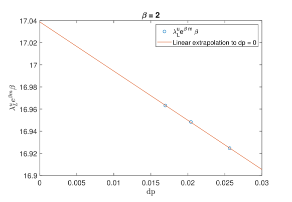
However, in a quantum system at a finite temperature, T, this norm can be evaluated in several ways. Let us denote ρ=eβH/Tr(eβH)𝜌superscript𝑒𝛽𝐻𝑇𝑟superscript𝑒𝛽𝐻\rho=e^{-\beta H}/Tr(e^{-\beta H}) as the thermal density matrix (β=1/T𝛽1𝑇\beta=1/T is the inverse temperature). For any 0α10𝛼10\leq\alpha\leq 1,

𝒞(α)(t,𝐱)=Tr(ρα[W𝟎(t),V𝐱]ρ(1α)[W𝟎(t),V𝐱]),subscript𝒞𝛼𝑡𝐱𝑇𝑟superscript𝜌𝛼superscriptsubscript𝑊0𝑡subscript𝑉𝐱superscript𝜌1𝛼subscript𝑊0𝑡subscript𝑉𝐱\mathcal{C}_{(\alpha)}(t,{\mathbf{x}})=Tr\left(\rho^{\alpha}[W_{\mathbf{0}}(t),V_{\mathbf{x}}]^{\dagger}\rho^{(1-\alpha)}[W_{\mathbf{0}}(t),V_{\mathbf{x}}]\right), (1)

is a Frobenius norm of the thermally smeared commutator ρ(1α)/2[W𝟎(t),V𝐱]ρα/2superscript𝜌1𝛼2subscript𝑊0𝑡subscript𝑉𝐱superscript𝜌𝛼2\rho^{(1-\alpha)/2}[W_{\mathbf{0}}(t),V_{\mathbf{x}}]\rho^{\alpha/2}, which encodes a notion of the size of operator spreading.
Refer to caption
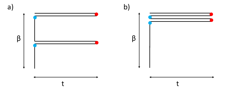
Figure 1: Contour for the (a) regulated and (b) unregulated out of time ordered correlators. The red points refer to the time evolved operators W𝟎(t)subscript𝑊0𝑡W_{\mathbf{0}}(t), and the blue points refer to the probe operators V𝐱subscript𝑉𝐱V_{\mathbf{x}}. The regulated and the unregulated correlators are distributed in distinct ways along the thermal circle.

Two choices of the squared commutator which have been studied in the literature, are the ‘regulated’ squared commutator, Cr(t,𝐱)=𝒞1/2(t,𝐱)subscript𝐶𝑟𝑡𝐱subscript𝒞12𝑡𝐱C_{r}(t,\mathbf{x})=\mathcal{C}_{1/2}(t,\mathbf{x}), and the ‘unregulated’ squared commutator, Cu(t,𝐱)=𝒞1(t,𝐱)subscript𝐶𝑢𝑡𝐱subscript𝒞1𝑡𝐱C_{u}(t,\mathbf{x})=\mathcal{C}_{1}(t,\mathbf{x}). When the expressions of the regulated and unregulated squared commutators are expanded, they contain terms which are thermally smeared versions of out of time ordered four point correlators of the form W𝟎(t)V𝐱W𝟎(t)V𝐱subscript𝑊0𝑡subscript𝑉𝐱subscript𝑊0𝑡subscript𝑉𝐱W_{\mathbf{0}}(t)V_{\mathbf{x}}W_{\mathbf{0}}(t)V_{\mathbf{x}}, evaluated on two distinct thermal contours, as shown in Fig. 1 a and b. In this work, we study these two squared commutators, and explore the difference in the physics that they capture Liao and Galitski (2018); Romero-Bermúdez et al. (2019).

I.2 Lyapunov exponent, butterfly velocity, and wavefront broadening

The squared commutator in holographic models, or in quantum systems with a semiclassical limit, grows exponentially at early times with a ‘Lyapunov exponent’ λLsubscript𝜆𝐿\lambda_{L}, 𝒞(t)eλLtsimilar-to𝒞𝑡superscript𝑒subscript𝜆𝐿𝑡\mathcal{C}(t)\sim e^{\lambda_{L}t}. In spatially local systems, the time argument can be replaced by the appropriate ttx/vB𝑡𝑡𝑥subscript𝑣𝐵t\to t-x/v_{B}, where vBsubscript𝑣𝐵v_{B} is a velocity determining the speed of information scrambling, called the ‘Butterfly velocity’ Roberts and Swingle (2016); Aleiner et al. (2016); Patel et al. (2017); Chowdhury and Swingle (2017). The butterfly velocity is state dependent analogue of the microscopic Lieb Robinson velocity Lieb and Robinson (1972).

However, interacting local quantum systems which are not in a semi-classical limit (that is, the number of local degrees of freedom is finite, and not large as in the case for systems with a semi-classical limit), show a qualitatively different behavior. As studies of random unitary circuits Nahum et al. (2018); von Keyserlingk et al. (2018), stochastic local Hamiltonian spin models Xu and Swingle (2019b), and numerical studies on deterministic quantum spin models Xu and Swingle (2019a); Khemani et al. (2018a); Sahu et al. (2019); Han and Hartnoll (2019) have shown, the near wave-front behavior of the squared commutator is,

𝒞(t,𝐱)exp(λ(x/vBt)1+ptp), for xvBt.similar-to𝒞𝑡𝐱𝜆superscript𝑥subscript𝑣𝐵𝑡1𝑝superscript𝑡𝑝, for 𝑥greater-than-or-equivalent-tosubscript𝑣𝐵𝑡\mathcal{C}(t,\mathbf{x})\sim\exp\left(-\lambda\frac{\left(x/v_{B}-t\right)^{1+p}}{t^{p}}\right)\text{, for }x\gtrsim v_{B}t. (2)

This behavior satisfies a ballistically growing and a broadening operator wavefront, xvBt+#tp/(1+p)similar-to𝑥subscript𝑣𝐵𝑡#superscript𝑡𝑝1𝑝x\sim v_{B}t+\#t^{p/(1+p)}, where vBsubscript𝑣𝐵v_{B} is the Butterfly velocity and p𝑝p is the broadening coefficient. For p=1𝑝1p=1, the broadening is diffusive, which is observed in the case of random unitary circuits Nahum et al. (2018); von Keyserlingk et al. (2018). This ballistic-diffusive form doesn’t exhibit an exponential ‘chaotic’ behavior. Until now, most studies of broadening were done at infinite temperature. However, unlike the ‘Lieb Robinson velocity’ of local quantum systems, the ‘Butterfly velocity’ is a state dependent information spreading velocity, and hence is a temperature dependent quantity. Furthermore the Lyapunov exponent and butterfly velocity could depend non-trivially on the choice of the contour. In this paper we explore these questions through a combination of numerical studies on quantum spin systems and analytical studies of tractable semi-classical field theory models.

I.3 Summary of our results

In this work we use a combination of numerical and analytical techniques to study the temperature and contour dependence of squared commutator in strongly interacting, gapped, local quantum systems. We do this firstly using a novel numerical technique based on matrix product operator (MPO) representation of Heisenberg operators to study scrambling in 1D quantum spin chains. We can access both the regulated and unregulated squared commutators in the early growth regime for a gapped, local Hamiltonian for large spin chains of 𝒪(200)𝒪200\mathcal{O}(200) spins upto long times t100J1similar-to𝑡100superscript𝐽1t\sim 100J^{-1}, where J1superscript𝐽1J^{-1} is the interaction scale of the Hamiltonian. Next, we study the low temperature behavior of the squared commutator in the paramagnetic phase of the 2+1D21𝐷2+1D non-linear O(N)𝑂𝑁O(N) model using perturbative calculation of the ladder-sum for the OTOC functions. We first list out the important results and the structure of the paper,

1. In Sec. II, we introduce the MPO numerical technique and apply it to calculate both the regulated and unregulated squared commutators in 1D mixed field Ising Hamiltonian. We observe a broadening of the expanding operator wave-front at all temperatures. This broadening behavior had been previously observed for the infinite T𝑇T ensemble Nahum et al. (2018); von Keyserlingk et al. (2018); Xu and Swingle (2019a); Khemani et al. (2018a); but here we confirm the persistence of the broadening behavior even at low temperatures.

For the regulated squared commutator we notice a strong temperature dependence of the broadening coefficient and butterfly velocity. We observe that at temperatures lower than the gap, β>m1𝛽superscript𝑚1\beta>m^{-1}, the butterfly velocity is consistent with a power-law ((βm)asuperscript𝛽𝑚𝑎(\beta m)^{-a} with a>0𝑎0a>0) behavior.

For the unregulated squared commutator, on the other hand, we observe that the butterfly velocity and the broadening coefficient have no observable temperature dependence, and in fact remain constant even as the temperature is tuned from β=0𝛽0\beta=0 to β>m1𝛽superscript𝑚1\beta>m^{-1}. This confirms a strong contour dependence of the OTOC Liao and Galitski (2018); Romero-Bermúdez et al. (2019). We also numerically study the contour dependence of tC(α)(t,𝐱)subscript𝑡subscript𝐶𝛼𝑡𝐱\partial_{t}C_{(\alpha)}(t,\mathbf{x}) and make a comparison with the chaos bound to demonstrate that the bound doesn’t apply to these squared commutators.

2. While the MPO technique can access temperatures below the gap, it is challenging to access very low temperatures. In order to calculate the temperature dependence at low temperatures, in Sec. III, we calculate the behavior of the regulated and unregulated squared commutator in the paramagnetic phase of the 2+1D21𝐷2+1D non-linear O(N)𝑂𝑁O(N) model. This is a gapped strongly interacting theory for which we can analytically calculate the scrambling behavior at large N𝑁N using a diagrammatic ladder technique. We find that the Lyapunov exponent is λLeβm/βsimilar-tosubscript𝜆𝐿superscript𝑒𝛽𝑚𝛽\lambda_{L}\sim e^{-\beta m}/\beta, and the butterfly velocity is vB(βm)1/2similar-tosubscript𝑣𝐵superscript𝛽𝑚12v_{B}\sim(\beta m)^{-1/2} at low temperatures such that β>>m1much-greater-than𝛽superscript𝑚1\beta>>m^{-1}. This shows that the butterfly velocity has the same scaling as the speed of sound of semiclassical massive particles. The field theory calculation can’t, however, reproduce the broadening behavior or the contour dependence, indicating that finite N corrections need to be taken into account for those features.

3. In Sec. IV, we summarize our results and compare the numerical and analytical approaches. We discuss the relation between the temperature dependence of butterfly velocity obtained in this paper with a recently derived temperature dependent bound on butterfly velocity Han and Hartnoll (2019). The bound is not sensitive to the contour dependence, and we show that it is consistent with temperature dependence of the butterfly velocities observed in Sec. II and III.

II Matrix product operator method for numerical calculation of scrambling

We now numerically study scrambling in a spatially local quantum system, consisting of tensor product of finite dimensional local Hilbert spaces, like spins on a lattice. The Hamiltonian is assumed to be a sum of geometrically local terms, and the lattice has a well defined position label.

Operators acting on vectors in a Hilbert space \mathcal{H} can be viewed as vectors on a ‘doubled’ Hilbert space LRtensor-productsubscript𝐿subscript𝑅\mathcal{H}_{L}\otimes\mathcal{H}_{R}. Here the tensor product structure refers to the two copies - ‘left’ and ‘right’ - of the state Hilbert spaces. We introduce the notation |..)|..) to denote the operator as a vector. A local operator acting on the 𝟎0\mathbf{0} position in the lattice, |W𝟎)|W_{\mathbf{0}}), can be time evolved in the Heisenberg picture,

|W𝟎(t))=|UtW𝟎Ut)=eit(HLIIHR)|W𝟎).|W_{\mathbf{0}}(t))=|U_{t}W_{\mathbf{0}}U_{t}^{\dagger})=e^{it(H_{L}\otimes I-I\otimes H^{*}_{R})}|W_{\mathbf{0}}). (3)

One can now probe the evolved operator using a second local operator at a position 𝐱𝐱\mathbf{x} by constructing its commutator,

|O(𝐱,t))=|[W𝟎(t),V𝐱])=(1V𝐱TV𝐱I)|W𝟎(t)),|O(\mathbf{x},t))=|[W_{\mathbf{0}}(t),V_{\mathbf{x}}])=(1\otimes V_{\mathbf{x}}^{T}-V_{\mathbf{x}}\otimes I)|W_{\mathbf{0}}(t)), (4)

The squared commutator can be obtained by squaring this operator which measures the extent of quantum information scrambling in the system. The α𝛼\alpha dependent squared commutator defined in Eq. 1 can be expressed as a norm of an operator state, 𝒞(α)=(Oα(𝐱,t,β)|Oα(𝐱,t,β))subscript𝒞𝛼conditionalsubscript𝑂𝛼𝐱𝑡𝛽subscript𝑂𝛼𝐱𝑡𝛽\mathcal{C}_{(\alpha)}=(O_{\alpha}(\mathbf{x},t,\beta)|O_{\alpha}(\mathbf{x},t,\beta)), where,

|Oα(𝐱,t,β))=|ρ(1α)/2O(𝐱,t)ρα/2).|O_{\alpha}(\mathbf{x},t,\beta))=|\rho^{(1-\alpha)/2}O(\mathbf{x},t)\rho^{\alpha/2}). (5)

II.1 Model and numerical method

We consider the mixed field quantum Ising model,

H=1E0(Ji=1L1ZiZi+1+hxi=1LXi+hzi=1LZi)𝐻1subscript𝐸0𝐽superscriptsubscript𝑖1𝐿1subscript𝑍𝑖subscript𝑍𝑖1subscript𝑥superscriptsubscript𝑖1𝐿subscript𝑋𝑖subscript𝑧superscriptsubscript𝑖1𝐿subscript𝑍𝑖H=-\frac{1}{E_{0}}\left(J\sum_{i=1}^{L-1}Z_{i}Z_{i+1}+h_{x}\sum_{i=1}^{L}X_{i}+h_{z}\sum_{i=1}^{L}Z_{i}\right) (6)

with E0=4J2+2hx2+2hz2subscript𝐸04superscript𝐽22superscriptsubscript𝑥22superscriptsubscript𝑧2E_{0}=\sqrt{4J^{2}+2h_{x}^{2}+2h_{z}^{2}}, on a one dimensional lattice. The X𝑋X and Z𝑍Z matrices are the usual Pauli matrices. The parameters chosen are, J=1,hx=1.05,hz=0.5formulae-sequence𝐽1formulae-sequencesubscript𝑥1.05subscript𝑧0.5J=1,h_{x}=1.05,h_{z}=0.5. Time is measured in the units of J1=1superscript𝐽11J^{-1}=1. This is a gapped system, and the spectral gap between the ground state and the first excited state is 1.13similar-toabsent1.13\sim 1.13 as extracted from small size exact diagonalization.

We want to calculate Cu,r(t,x)subscript𝐶𝑢𝑟𝑡𝑥C_{u,r}(t,x) for large system sizes and upto long times, and we employ the Matrix product operators (MPO) based technique to time evolve operator states which extends the time dependent density matrix renormalization group (t-DMRG) technique Vidal (2003, 2004); Daley et al. (2004); White and Feiguin (2004) to super-operators Xu and Swingle (2019a). We first time evolve the local operator W𝑊W by doing time evolution using super-operator HIIHtensor-product𝐻𝐼tensor-product𝐼superscript𝐻H\otimes I-I\otimes H^{*} on the operator state, following Eq. 3. We also obtain |ρ)|\rho) by evolving the identity |I)|I) operator state in imaginary time. Now, we can construct the operator state |Oα(t,𝐱,β))|O_{\alpha}(t,\mathbf{x},\beta)) as defined in Eq. 5, for α=1/2(1)𝛼121\alpha=1/2(1), and its norm squared is the required (un)regulated squared commutator.

In the MPO based method, at each Trotter step, we must truncate the MPO to a fixed bond dimension, thereby introducing errors. However, we will demonstrate that our numerical procedure converges (for small values of the squared commutator) at large system sizes (L200similar-to𝐿200L\sim 200) and upto long times t100similar-to𝑡100t\sim 100, even at low temperatures, which makes it a powerful method to study the temperature and contour dependence of quantum information scrambling.
Refer to caption
Refer to caption
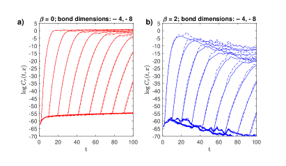
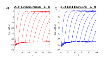
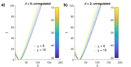
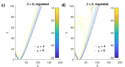
Figure 2: The contours of the logarithm of the regulated and unregulated squared commutator at different temperatures - a) β=0𝛽0\beta=0 (unregulated), b) β=2𝛽2\beta=2 (unregulated), c) β=0𝛽0\beta=0 (regulated) and d) β=2𝛽2\beta=2 (regulated) are shown. For the unregulated case bond dimensions, χ=8𝜒8\chi=8 and χ=16𝜒16\chi=16, and for the regulated case bond dimensions, χ=4𝜒4\chi=4 and χ=8𝜒8\chi=8 are considered. The data shows convergence even at low temperatures for logCr<30subscript𝐶𝑟30\log C_{r}<-30, and for logCu<20subscript𝐶𝑢20\log C_{u}<-20.

We consider a L=200𝐿200L=200 spin chain with the mixed field Ising Hamiltonian as in Eq. 6. We start with an operator X20subscript𝑋20X_{20}, a Pauli X𝑋X operator localized at the site 202020, and construct the squared commutator with Z𝑍Z operators at all sites of the chain. We perform the MPO-TEBD method with Trotter steps, δt=0.005𝛿𝑡0.005\delta t=0.005 for time evolution (to generate X(t)𝑋𝑡X(t)) and δβ=0.05𝛿𝛽0.05\delta\beta=0.05 for imaginary time evolution (to generate ρ𝜌\rho), for bond dimensions χ=4,8𝜒48\chi=4,8 (regulated) and χ=8,16𝜒816\chi=8,16 (unregulated). To calculate the regulated and unregulated squared commutators, we need to construct the MPOs |O1/2(t,x,β))|O_{1/2}(t,x,\beta)) and |O1(t,x,β))|O_{1}(t,x,\beta)), as defined in Eq. 5, respectively. For |O1/2)|O_{1/2}) we need to perform two MPO multiplications, ρ1/4[X20(t),Zx]ρ1/4ρ1/4[X20(t),Zx]ρ1/4superscript𝜌14subscript𝑋20𝑡subscript𝑍𝑥superscript𝜌14superscript𝜌14subscript𝑋20𝑡subscript𝑍𝑥superscript𝜌14\rho^{1/4}\to[X_{20}(t),Z_{x}]\rho^{1/4}\to\rho^{1/4}[X_{20}(t),Z_{x}]\rho^{1/4}, while for |O1)|O_{1}), we need to perform one MPO multiplication, ρ1/2[X20(t),Zx]ρ1/2superscript𝜌12subscript𝑋20𝑡subscript𝑍𝑥superscript𝜌12\rho^{1/2}\to[X_{20}(t),Z_{x}]\rho^{1/2}. The details of the numerical implementation, which include a comparison to exact diagonalization, discussions on convergence with bond dimension, and the fitting procedure, are provided in App. A.

A heuristic justification of why the MPO approximation works is as follows - it was shown in Xu and Swingle (2019a) that the commutator [X(t),Zx]𝑋𝑡subscript𝑍𝑥[X(t),Z_{x}] has a small operator entanglement outside the light-cone. It is also well understood that the thermal density matrix ρ𝜌\rho satisfies an area law in mutual information Wolf et al. (2008), and hence is expected to be reliably approximated by a low bond dimension matrix product operator. These two arguments imply that the operator |Oα(t,𝐱,β))|O_{\alpha}(t,\mathbf{x},\beta)) as defined in Eq. 5, which is an MPO multiplication of powers of ρ𝜌\rho and the commutator [X(t),Zx]𝑋𝑡subscript𝑍𝑥[X(t),Z_{x}], should have a small operator entanglement outside the light-cone (i.e. when the squared commutator is small), and hence can be well approximated by a low bond dimension MPO.

As has been pointed out previously, in Xu and Swingle (2019a); Hémery et al. (2019); Sahu et al. (2019), the MPO-TEBD method can capture the qualitative features of scrambling only if the scrambling data has converged with bond dimension. We ensure that all our further analysis is done on scrambling data only in the spatio-temporal domain where it has converged with bond dimension. We plot the contours of the squared commutator in Fig. 2, and demonstrate that the contours converge very well for small values of the squared commutator. The shape of the contours, where the data has converged, show that the wavefront propagates ballistically with a velocity.

II.2 Broadening of the wavefront
Refer to caption
Refer to caption
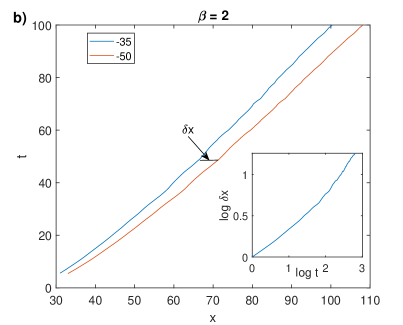
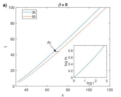
Figure 3: We extract the contours of logCr=35subscript𝐶𝑟35\log C_{r}=-35 and 5050-50 at different temperatures, for the data with χ=8𝜒8\chi=8. From the contours we extract δx𝛿𝑥\delta x, which is the spatial distance between the two contours. The time dependence of δx𝛿𝑥\delta x is shown in the inset; the fact that it is increasing with time demonstrates a broadening of the wavefront. The broadening persists even at a) high temperature β=0𝛽0\beta=0 and b) low temperature β=2𝛽2\beta=2.

Without any numerical fitting, we demonstrate the broadening behavior of the operator wavefront even at low temperatures in the Fig. 3. We extract the spatial separation δx𝛿𝑥\delta x between two chosen contours of the logCrsubscript𝐶𝑟\log C_{r}, and plot its time dependence in the insets of Fig. 3. A positive (and an increasing) slope implies a broadening behavior. In Fig. 3, we show data for the regulated case, but a similar study for the unregulated squared commutator also demonstrates a broadening behavior. Thus, the Figs. 2 and 3 together show that the early time (before the light-cone is reached) behavior of the squared commutator has a ballistic growth and a broadening wavefront.

In Xu and Swingle (2019a, b); Khemani et al. (2018b), it was argued that the squared commutator, near the wavefront, when C(x,t)<<1much-less-than𝐶𝑥𝑡1C(x,t)<<1, can be captured by the following ansatz,

C(x,t)exp(λp((xx0)/vBt)1+ptp).similar-to𝐶𝑥𝑡𝑒𝑥𝑝subscript𝜆𝑝superscript𝑥subscript𝑥0subscript𝑣𝐵𝑡1𝑝superscript𝑡𝑝C(x,t)\sim exp\left(-\lambda_{p}\frac{\left((x-x_{0})/v_{B}-t\right)^{1+p}}{t^{p}}\right). (7)

One can identify the broadening coefficient p𝑝p as,

δlogδxδtpp+1.similar-to𝛿𝛿𝑥𝛿𝑡𝑝𝑝1\frac{\delta\log\delta x}{\delta t}\sim\frac{p}{p+1}. (8)

We now fit our data to the ansatz in Eq. 7 to extract the Lyapunov exponent, butterfly velocity and broadening coefficient.

II.3 Temperature dependence of butterfly velocity
Refer to caption
Refer to caption
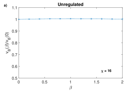
Figure 4: a) We plot the extracted vB(β)/vB(0)subscript𝑣𝐵𝛽subscript𝑣𝐵0v_{B}(\beta)/v_{B}(0) for the unregulated case, as a function of β𝛽\beta. The data is for χ=16𝜒16\chi=16 bond dimension. The butterfly velocity is practically constant at all temperatures. b) For the regulated case, we plot the normalized vBsubscript𝑣𝐵v_{B}, (i.e. vB(β)/vB(0)subscript𝑣𝐵𝛽subscript𝑣𝐵0v_{B}(\beta)/v_{B}(0)), extracted from the χ=8𝜒8\chi=8 data, as a function of β𝛽\beta. In the inset, in the log-log scale, we demonstrate that the low temperature behavior of vBsubscript𝑣𝐵v_{B} is consistent with β1/2superscript𝛽12\beta^{-1/2} (which is the slope of the red line plotted.).

We extract the butterfly velocity, velocity dependent Lyapunov exponent and the broadening coefficient from the obtained numerical data by fitting them to the near wave-front ansatz in Eq. 7. In Fig. 4a, we plot fitted vB(β)/vB(0)subscript𝑣𝐵𝛽subscript𝑣𝐵0v_{B}(\beta)/v_{B}(0) as a function of β𝛽\beta for the unregulated case, and see that the fitted butterfly velocity has almost no discernible temperature dependence. In Fig. 4b, we plot the same for the regulated case, and notice a strong temperature dependence. The low temperature behavior is consistent with a power law decrease in the butterfly velocity as a function of β𝛽\beta, as is shown in the inset of Fig. 4b. In Sec. III, we show that at the low temperature limit of an analytically tractable field theory model with a mass gap m𝑚m, the butterfly velocity has a temperature scaling which is the same as the equipartition behavior - 1/βm1𝛽𝑚\sqrt{1/\beta m}. The asymptotic low temperature behavior in the MPO calculation (even though the temperatures we access here are not very low compared to the spectral gap) is close to the 1/βm1𝛽𝑚\sqrt{1/\beta m} behavior, as is demonstrated in Fig. 4b.

In App. A, we also study the temperature dependence of the broadening coefficient p𝑝p. In Fig. 15, we show that p𝑝p for the unregulated case has a very weak dependence on temperature and remains practically constant as the temperature is lowered. The regulated case, however, has an increasing trend for p𝑝p with decreasing temperature.

II.4 Contour dependence and chaos bound

Refer to caption
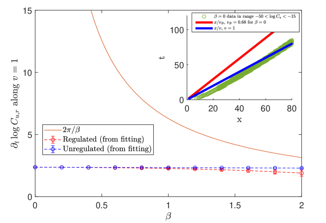
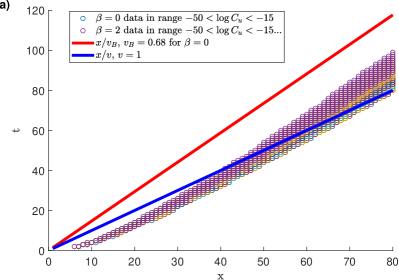
Figure 5: From the fitting of the obtained data of the regulated and unregulated squared commutators, we obtain the tCu,rsubscript𝑡subscript𝐶𝑢𝑟\partial_{t}C_{u,r} from the near wavefront ansatz, along a ‘ray’ x=t𝑥𝑡x=t and compare it against the ‘bound on chaos’ 2π/β2𝜋𝛽2\pi/\beta. In the inset, we show the ‘ray’ x=vt𝑥𝑣𝑡x=vt at v=1𝑣1v=1, and compare that to the butterfly velocity vB=0.68subscript𝑣𝐵0.68v_{B}=0.68 at β=0𝛽0\beta=0 for Cusubscript𝐶𝑢C_{u}.

For a symmetrically defined out of time ordered correlation function, there exists the Maldacena-Shenker-Stanford (MSS) chaos bound λL2π/βsubscript𝜆𝐿2𝜋𝛽\lambda_{L}\leq 2\pi/\beta Maldacena et al. (2016). The symmetric OTOC is defined as,

F(t,𝐱)=Tr(ρ1/4V𝐱ρ1/4W0(t)ρ1/4V𝐱ρ1/4W0(t)).𝐹𝑡𝐱𝑇𝑟superscript𝜌14subscript𝑉𝐱superscript𝜌14subscript𝑊0𝑡superscript𝜌14subscript𝑉𝐱superscript𝜌14subscript𝑊0𝑡F(t,\mathbf{x})=Tr\left(\rho^{1/4}V_{\mathbf{x}}\rho^{1/4}W_{0}(t)\rho^{1/4}V_{\mathbf{x}}\rho^{1/4}W_{0}(t)\right). (9)

This is related to the regulated squared commutator, as the Cr(t,𝐱)subscript𝐶𝑟𝑡𝐱C_{r}(t,\mathbf{x}), when expanded,

Cr(t,𝐱)=2(Tr(ρ1/2V𝐱W0(t)ρ1/2W0(t)V𝐱)ReF(t+iβ/4,𝐱)).subscript𝐶𝑟𝑡𝐱2𝑇𝑟superscript𝜌12subscript𝑉𝐱subscript𝑊0𝑡superscript𝜌12subscript𝑊0𝑡subscript𝑉𝐱𝑅𝑒𝐹𝑡𝑖𝛽4𝐱C_{r}(t,\mathbf{x})=2\left(Tr\left(\rho^{1/2}V_{\mathbf{x}}W_{0}(t)\rho^{1/2}W_{0}(t)V_{\mathbf{x}}\right)-ReF(t+i\beta/4,\mathbf{x})\right). (10)

Let’s introduce a related quantity Fd(t,𝐱)=Tr(ρ1/2V𝐱ρ1/2V𝐱)Tr(ρ1/2W0(tρ1/2W0(t)F_{d}(t,\mathbf{x})=Tr\left(\rho^{1/2}V_{\mathbf{x}}\rho^{1/2}V_{\mathbf{x}}\right)Tr\left(\rho^{1/2}W_{0}(t\rho^{1/2}W_{0}(t\right). In Maldacena et al. (2016), it was proven that the following bound exists,

log(Fd(t,𝐱)F(t,𝐱))t2πβ.subscript𝐹𝑑𝑡𝐱𝐹𝑡𝐱𝑡2𝜋𝛽\frac{\partial\log\left(F_{d}(t,\mathbf{x})-F(t,\mathbf{x})\right)}{\partial t}\leq\frac{2\pi}{\beta}. (11)

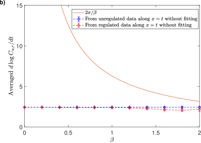
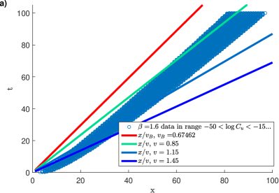
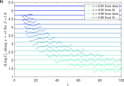
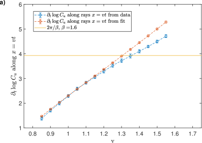
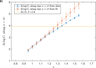
Given this result, one might conjecture that the related quantity tlogCr(t,𝐱)subscript𝑡subscript𝐶𝑟𝑡𝐱\partial_{t}\log C_{r}(t,\mathbf{x}) also satisfies the same bound. To study this, we can calculate tlogCr(t,𝐱)subscript𝑡subscript𝐶𝑟𝑡𝐱\partial_{t}\log C_{r}(t,\mathbf{x}) along different ‘rays’ x=vt𝑥𝑣𝑡x=vt Khemani et al. (2018a); if the near wavefront scrambling ansatz (Eq. 7) is satisfied, then tlogCu,rsubscript𝑡subscript𝐶𝑢𝑟\partial_{t}\log C_{u,r} along a ray of velocity v𝑣v is given by λp(v/vB1)p(1+pv/vB)subscript𝜆𝑝superscript𝑣subscript𝑣𝐵1𝑝1𝑝𝑣subscript𝑣𝐵\lambda_{p}(v/v_{B}-1)^{p}(1+pv/v_{B}). At sufficiently large v𝑣v, this will violate the chaos bound. In Fig. 5, we plot the tlogCr,u(t,𝐱)subscript𝑡subscript𝐶𝑟𝑢𝑡𝐱\partial_{t}\log C_{r,u}(t,\mathbf{x}), for a fixed ‘ray’ x=t𝑥𝑡x=t, obtained from fitting of the unregulated and regulated cases to the ansatz, as a function of β𝛽\beta and notice that the unregulated case is practically constant, and can violate the bound at lower temperatures. We confirm this without numerical fitting, in App. B, Fig. 16. In App. B we also study tlogCr,u(t,x=vt)subscript𝑡subscript𝐶𝑟𝑢𝑡𝑥𝑣𝑡\partial_{t}\log C_{r,u}(t,x=vt), as a function of ‘ray’ velocity v𝑣v. We find that at high ray velocities v𝑣v, both tlogCr(t,vt)subscript𝑡subscript𝐶𝑟𝑡𝑣𝑡\partial_{t}\log C_{r}(t,vt) and tlogCu(t,vt)subscript𝑡subscript𝐶𝑢𝑡𝑣𝑡\partial_{t}\log C_{u}(t,vt) violate the bound. This shows that the MSS bound doesn’t hold for the squared commutators we considered.

II.5 Summary of findings from the MPO numerics

By studying squared commutators for large-sized, gapped spin chain which is spatially local, and has finite dimensional local Hilbert spaces, we got three distinctive features. First, the spatial locality leads to a ballistic wavefront propagating at the butterfly velocity, which has distinct temperature scaling for the regulated and unregulated cases. In the unregulated case the velocity is constant, while for the regulated case, the velocity decreases with temperature. Second, the wavefront broadens with time for both contours, and thus the squared commutator doesn’t have pure exponential growth. Third, there are numerical indications that the chaos bound is not satisfied for these squared commutators.

Can we explain these behaviors using an analytically tractable model? In particular, can we understand the low temperature limit which is not accessible in the spin chain numerics? We explore that in the next section, where we consider a non-linear O(N)𝑂𝑁O(N) model in 2+1D21𝐷2+1D, which is spatially local, and solvable at large N𝑁N. We study the scrambling behavior at low temperatures for the gapped phase of the model, and find that the butterfly velocity indeed varies as T/m𝑇𝑚\sqrt{T/m} at low temperatures. However, we will find that the field theory calculation doesn’t show contour dependence or wavefront broadening.

{fmffile}

whole_file

III Scrambling in the paramagnetic phase of the non-linear O(N)𝑂𝑁O(N) model

Refer to caption
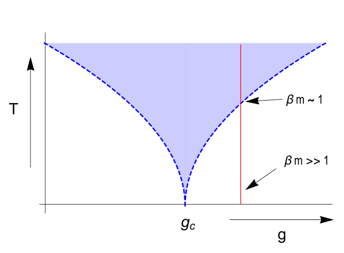
Figure 6: This is the critical phase diagram of the non-linear O(N)𝑂𝑁O(N) model. The blue shaded region is controlled by the critical theory around the quantum critical point at T=0𝑇0T=0 and g=gc𝑔subscript𝑔𝑐g=g_{c}, while the dashed lines indicate a cross-over to the phases controlled by the symmetry of the zero temperature phases away from the critical point. We focus on the low temperature behavior of the symmetry unbroken paramagnetic phase g>gc𝑔subscript𝑔𝑐g>g_{c}.

The non-linear O(N)𝑂𝑁O(N) model is a spatially local field theory of an O(N)𝑂𝑁O(N) symmetric vector field ϕasubscriptitalic-ϕ𝑎\phi_{a}, with a=1,..,Na=1,..,N. The theory is solvable at large N𝑁N, and in this limit this model differs from the spin chain in the fact that the local Hilbert space is not finite. Furthermore, to avoid complications in the field theory at 1+1D11𝐷1+1D due to scattering, we study this model at 2+1D21𝐷2+1D, and we expect that dimensionality will not affect qualitative features of the temperature and contour dependence. The critical phase diagram Sachdev (2011) of this model is shown in Fig. 6. We analyse this model using Ladder sum techniques developed in Stanford (2016); Chowdhury and Swingle (2017) (see also Steinberg and Swingle (2019); Cheng and Swingle (2019); Alavirad and Lavasani (2019); Gu and Kitaev (2019)), and study both the temperature and contour dependence of the squared commutators.

The real time lagrangian for this theory is given by,

=12[a(ϕa)2v2N(ϕa2Ng)2]12delimited-[]subscript𝑎superscriptsubscriptitalic-ϕ𝑎2𝑣2𝑁superscriptsuperscriptsubscriptitalic-ϕ𝑎2𝑁𝑔2\mathcal{L}=\frac{1}{2}\left[\sum_{a}(\partial\phi_{a})^{2}-\frac{v}{2N}\left(\phi_{a}^{2}-\frac{N}{g}\right)^{2}\right] (12)

The action is given by xsubscript𝑥\int_{x}\mathcal{L}, where the space-time integration xsubscript𝑥\int_{x} is over 2+1D21𝐷2+1D. We have set the speed of light c𝑐c and Planck-constant-over-2-pi\hbar to 1. The parameter g𝑔g (which determines the bare mass) can be tuned across a quantum critical point that occurs at g=gc𝑔subscript𝑔𝑐g=g_{c}, and v𝑣v is the self-interaction coupling constant. We consider the strong coupling (large v𝑣v) and large-N𝑁N limit. In Chowdhury and Swingle (2017), scrambling behavior was studied at the critical point gcsubscript𝑔𝑐g_{c}, by evaluating the regulated squared commutator using a perturbative ladder sum calculation with 1/N1𝑁1/N as the small parameter Stanford (2016); Chowdhury and Swingle (2017). Following the diagrammatic techniques used in these studies, we study scrambling on the paramagnetic phase of the model at g>gc𝑔subscript𝑔𝑐g>g_{c}, where there are quasiparticle-like excitations with finite bare mass m𝑚m. We study the temperature dependence of the scrambling in the low temperature limit βm>>1much-greater-than𝛽𝑚1\beta m>>1.

The main goal of this section is to analytically obtain temperature dependence of the butterfly velocity at low temperatures. We didn’t have access to very low temperatures in Sec. II, and we intend to explore the regime βm>>1much-greater-than𝛽𝑚1\beta m>>1 using this field theory model.

The generalized squared commutator in different contours given in Fig. 1 is given by,

Cα(t,𝐱)=1N2abTr(ρα[ϕa(t,𝟎),ϕb(0,𝐱)]ρ1α[ϕa(t,𝟎),ϕb(0,𝐱)]).subscript𝐶𝛼𝑡𝐱1superscript𝑁2subscript𝑎𝑏𝑇𝑟superscript𝜌𝛼subscriptitalic-ϕ𝑎𝑡0subscriptitalic-ϕ𝑏0𝐱superscript𝜌1𝛼subscriptitalic-ϕ𝑎𝑡0subscriptitalic-ϕ𝑏0𝐱C_{\alpha}(t,\mathbf{x})=-\frac{1}{N^{2}}\sum_{ab}Tr\left(\rho^{\alpha}[\phi_{a}(t,\mathbf{0}),\phi_{b}(0,\mathbf{x})]\rho^{1-\alpha}[\phi_{a}(t,\mathbf{0}),\phi_{b}(0,\mathbf{x})]\right). (13)

The regulated and the unregulated squared commutators are given by Cr=C1/2subscript𝐶𝑟subscript𝐶12C_{r}=C_{1/2}, and Cu=C1subscript𝐶𝑢subscript𝐶1C_{u}=C_{1}, respectively.

We summarize the results of this section before showing the explicit calculations. Using the ladder-sum calculation, we find that both the regulated and unregulated squared commutators have the following early time behavior,

Cr,u(t,𝐱)1Neλ0(tx2vBt),similar-tosubscript𝐶𝑟𝑢𝑡𝐱1𝑁superscript𝑒subscript𝜆0𝑡superscript𝑥2subscript𝑣𝐵𝑡C_{r,u}(t,\mathbf{x})\sim\frac{1}{N}e^{\lambda_{0}\left(t-\frac{x^{2}}{v_{B}t}\right)}, (14)

where the ‘Lyapunov’ exponent, λ0eβm/βsimilar-tosubscript𝜆0superscript𝑒𝛽𝑚𝛽\lambda_{0}\sim e^{-\beta m}/\beta, and the butterfly velocity, vB(βm)1/2similar-tosubscript𝑣𝐵superscript𝛽𝑚12v_{B}\sim(\beta m)^{-1/2}. This implies that at low temperatures, the butterfly velocity has the same temperature scaling as the speed of sound (which also scales as (βm)1/2superscript𝛽𝑚12(\beta m)^{-1/2}) of the semi-classical gas of dilute quasiparticle excitations of the paramagnetic phase of the O(N)𝑂𝑁O(N) model at low temperature.

III.1 Basic diagrammatics and low temperature relaxation rate

We introduce auxiliary Hubbard Stratonovich (HS) field λ𝜆\lambda to solve the interacting problem. The Euclidean Lagrangian we consider is

E=12[a(ϕa)2λN(aϕa2Ng)λ24v]subscript𝐸12delimited-[]subscript𝑎superscriptsubscriptitalic-ϕ𝑎2𝜆𝑁subscript𝑎superscriptsubscriptitalic-ϕ𝑎2𝑁𝑔superscript𝜆24𝑣\mathcal{L}_{E}=\frac{1}{2}\left[\sum_{a}(\partial\phi_{a})^{2}-\frac{\lambda}{\sqrt{N}}\left(\sum_{a}\phi_{a}^{2}-\frac{N}{g}\right)-\frac{\lambda^{2}}{4v}\right] (15)

The HS field λ𝜆\lambda is chosen so that it generates a zero temperature mass, m𝑚m, such that, λN=m2delimited-⟨⟩𝜆𝑁superscript𝑚2\frac{-\langle\lambda\rangle}{\sqrt{N}}=m^{2}. The HS field also acts as a Lagrange multiplier, fixing (at large N), ϕa2=Ngdelimited-⟨⟩superscriptsubscriptitalic-ϕ𝑎2𝑁𝑔\langle\sum\phi_{a}^{2}\rangle=\frac{N}{g}. At finite temperature T𝑇T, the constraint imposed by the HS field is

NTiωn𝐤Λ1ωn2+ϵ𝐤2=Ng, where ϵ𝐤=𝐤2+m2.formulae-sequence𝑁𝑇subscript𝑖subscript𝜔𝑛superscriptsubscript𝐤Λ1superscriptsubscript𝜔𝑛2superscriptsubscriptitalic-ϵ𝐤2𝑁𝑔 where subscriptitalic-ϵ𝐤superscript𝐤2superscript𝑚2\begin{split}&NT\sum_{i\omega_{n}}\int_{\mathbf{k}}^{\Lambda}\frac{1}{\omega_{n}^{2}+\epsilon_{\mathbf{k}}^{2}}=\frac{N}{g},\text{ where }\epsilon_{\mathbf{k}}=\sqrt{\mathbf{k}^{2}+m^{2}}.\end{split} (16)

Here, and in the rest of the paper, 𝐩subscript𝐩\int_{\mathbf{p}} stands for d2𝐩(2π)2superscript𝑑2𝐩superscript2𝜋2\int\frac{d^{2}\mathbf{p}}{(2\pi)^{2}}. At β=1T=𝛽1𝑇\beta=\frac{1}{T}=\infty, this fixes g𝑔g in terms of m𝑚m and ΛΛ\Lambda,

14π(Λm)=1g14𝜋Λ𝑚1𝑔\frac{1}{4\pi}(\Lambda-m)=\frac{1}{g} (17)

At finite temperature, the mass will be modified, as a function m(β)𝑚𝛽m(\beta). We restrict ourselves to low temperature, assuming the hierarchy of scales Λ>>m>>β1much-greater-thanΛ𝑚much-greater-thansuperscript𝛽1\Lambda>>m>>\beta^{-1}. This implies m(β)m𝑚𝛽𝑚m(\beta)\approx m, i.e., the thermal mass is approximately the same as the bare mass.

The perturbative calculation of the squared commutator can be set up using the basic ingredients - the real time retarded and Wightman propagators of the fields ϕasubscriptitalic-ϕ𝑎\phi_{a} and the HS field λ𝜆\lambda. The retarded propagators are identified as horizontal lines, while the Wightman propagators are denoted as the vertical lines in the diagrams (in momentum space).

For the ϕitalic-ϕ\phi field, bare Euclidean propagator in imaginary time τ𝜏\tau is 𝒢(τ,𝐱)=Tr(ρϕa(τ,𝐱)ϕb(0,𝟎))𝒢𝜏𝐱𝑇𝑟𝜌subscriptitalic-ϕ𝑎𝜏𝐱subscriptitalic-ϕ𝑏00\mathcal{G}(\tau,\mathbf{x})=Tr\left(\rho\phi_{a}(\tau,\mathbf{x})\phi_{b}(0,\mathbf{0})\right), where, ρ𝜌\rho is the thermal density matrix, ρ=eβH/(Z=Tr(eβH))𝜌superscript𝑒𝛽𝐻𝑍𝑇𝑟superscript𝑒𝛽𝐻\rho=e^{-\beta H}/(Z=Tr(e^{-\beta H})). The retarded propagator is defined as 𝒢R(t,𝐱)δab=iTr(ρ[ϕa(t,𝐱),ϕb(0,𝟎)])θ(t)subscript𝒢𝑅𝑡𝐱subscript𝛿𝑎𝑏𝑖𝑇𝑟𝜌subscriptitalic-ϕ𝑎𝑡𝐱subscriptitalic-ϕ𝑏00𝜃𝑡\mathcal{G}_{R}(t,\mathbf{x})\delta_{ab}=-iTr\left(\rho[\phi_{a}(t,\mathbf{x}),\phi_{b}(0,\mathbf{0})]\right)\theta(t). In the Fourier space, they are related by analytic continuation of the Matsubara frequencies, 𝒢R(ω,𝐤)=𝒢(iωnω,𝐤)subscript𝒢𝑅𝜔𝐤𝒢𝑖subscript𝜔𝑛𝜔𝐤\mathcal{G}_{R}(\omega,\mathbf{k})=-\mathcal{G}(i\omega_{n}\to\omega,\mathbf{k}). We can calculate and denote the retarded bare propagator as,

{fmfgraph} (40,15) \fmflefti \fmfrighto \fmfplain,width=0.5pti,o :=𝒢R(0)(ω,𝐤)=1(ω+i0+)2ϵ𝐤2.\begin{split}\parbox{56.9055pt}{\fmfgraph(40,15) \fmfleft{i} \fmfright{o} \fmf{plain,width=0.5pt}{i,o} }&:=\quad\mathcal{G}^{(0)}_{R}(\omega,\mathbf{k})=\frac{1}{(\omega+i0^{+})^{2}-\epsilon_{\mathbf{k}}^{2}}.\end{split} (18)

The spectral function is defined as A(ω,𝐤)=2Im[𝒢R(ω,𝐤)]𝐴𝜔𝐤2𝐼𝑚delimited-[]subscript𝒢𝑅𝜔𝐤A(\omega,\mathbf{k})=-2Im[\mathcal{G}_{R}(\omega,\mathbf{k})]. The bare ϕitalic-ϕ\phi spectral function is given by,

A(0)(ω,𝐤)=πϵ𝐤[δ(ωϵ𝐤)δ(ω+ϵ𝐤)].superscript𝐴0𝜔𝐤𝜋subscriptitalic-ϵ𝐤delimited-[]𝛿𝜔subscriptitalic-ϵ𝐤𝛿𝜔subscriptitalic-ϵ𝐤A^{(0)}(\omega,\mathbf{k})=\frac{\pi}{\epsilon_{\mathbf{k}}}[\delta(\omega-\epsilon_{\mathbf{k}})-\delta(\omega+\epsilon_{\mathbf{k}})]. (19)

The generalized Wightman function is defined as,

𝒢W(α)(t,𝐱)δab:=Tr(ραϕa(t,𝐱)ρ1αϕb(0,𝟎)).assignsubscriptsuperscript𝒢𝛼𝑊𝑡𝐱subscript𝛿𝑎𝑏𝑇𝑟superscript𝜌𝛼subscriptitalic-ϕ𝑎𝑡𝐱superscript𝜌1𝛼subscriptitalic-ϕ𝑏00\mathcal{G}^{(\alpha)}_{W}(t,\mathbf{x})\delta_{ab}:=Tr\left(\rho^{\alpha}\phi_{a}(t,\mathbf{x})\rho^{1-\alpha}\phi_{b}(0,\mathbf{0})\right). (20)

By going to the spectral representation, we show in App. C,

𝒢W(α)(ω,𝐤)=A(ω,𝐤)2sinhβω2e(α1/2)βω.subscriptsuperscript𝒢𝛼𝑊𝜔𝐤𝐴𝜔𝐤2𝛽𝜔2superscript𝑒𝛼12𝛽𝜔\mathcal{G}^{(\alpha)}_{W}(\omega,\mathbf{k})=\frac{A(\omega,\mathbf{k})}{2\sinh\frac{\beta\omega}{2}}e^{(\alpha-1/2)\beta\omega}. (21)

For the λ𝜆\lambda field, the bare Euclidean propagator is 𝒢λ(0)(iωn,𝐤)=4vsuperscriptsubscript𝒢𝜆0𝑖subscript𝜔𝑛𝐤4𝑣\mathcal{G}_{\lambda}^{(0)}(i\omega_{n},\mathbf{k})=-4v. At infinite v𝑣v, one can dress the λ𝜆\lambda propagators as shown in Fig. 7. In that case,

𝒢λ(iωn,𝐤)=𝒢λ01Π𝒢λ0v1Π(iωn,𝐤),subscript𝒢𝜆𝑖subscript𝜔𝑛𝐤superscriptsubscript𝒢𝜆01Πsuperscriptsubscript𝒢𝜆0subscript𝑣1Π𝑖subscript𝜔𝑛𝐤\mathcal{G}_{\lambda}(i\omega_{n},\mathbf{k})=\frac{\mathcal{G}_{\lambda}^{0}}{1-\Pi\mathcal{G}_{\lambda}^{0}}\underbrace{\longrightarrow}_{v\to\infty}-\frac{1}{\Pi(i\omega_{n},\mathbf{k})}, (22)

where ΠΠ\Pi is the one loop ϕitalic-ϕ\phi bubble,

Π(iνn,𝐤)Π𝑖subscript𝜈𝑛𝐤\displaystyle\Pi(i\nu_{n},\mathbf{k}) =T2iωn𝐪Λ1(ωn+νn)2+ϵ𝐪+𝐤21ωn2+ϵ𝐪2.absent𝑇2subscript𝑖subscript𝜔𝑛superscriptsubscript𝐪Λ1superscriptsubscript𝜔𝑛subscript𝜈𝑛2superscriptsubscriptitalic-ϵ𝐪𝐤21superscriptsubscript𝜔𝑛2superscriptsubscriptitalic-ϵ𝐪2\displaystyle=\frac{T}{2}\sum_{i\omega_{n}}\int_{\mathbf{q}}^{\Lambda}\frac{1}{(\omega_{n}+\nu_{n})^{2}+\epsilon_{\mathbf{q}+\mathbf{k}}^{2}}\frac{1}{\omega_{n}^{2}+\epsilon_{\mathbf{q}}^{2}}. (23)

The retarded polarization bubble is given by analytic continuation, ΠR(ω,𝐤)=Π(iωnω,𝐤)subscriptΠ𝑅𝜔𝐤Π𝑖subscript𝜔𝑛𝜔𝐤\Pi_{R}(\omega,\mathbf{k})=\Pi(i\omega_{n}\to\omega,\mathbf{k}). The resummed retarded λ𝜆\lambda propagator is then denoted as,

{fmfgraph} (40,15) \fmflefti \fmfrighto \fmfdashes,width=2pti,o :=𝒢R,λ(ω,𝐤)=1ΠR(ω,𝐤).\parbox{56.9055pt}{\fmfgraph(40,15) \fmfleft{i} \fmfright{o} \fmf{dashes,width=2pt}{i,o} }:=\quad\mathcal{G}_{R,\lambda}(\omega,\mathbf{k})=\frac{1}{\Pi_{R}(\omega,\mathbf{k})}. (24)

From the λ𝜆\lambda spectral function, Aλ(ω,𝐤)=2Im[𝒢R(ω,𝐤)]subscript𝐴𝜆𝜔𝐤2𝐼𝑚delimited-[]subscript𝒢𝑅𝜔𝐤A_{\lambda}(\omega,\mathbf{k})=-2Im[\mathcal{G}_{R}(\omega,\mathbf{k})], we can define the generalized λ𝜆\lambda Wightman function,

𝒢W,λ(α)(ω,𝐤)=Aλ(ω,𝐤)2sinhβω2e(α1/2)βω.superscriptsubscript𝒢𝑊𝜆𝛼𝜔𝐤subscript𝐴𝜆𝜔𝐤2𝛽𝜔2superscript𝑒𝛼12𝛽𝜔\mathcal{G}_{W,\lambda}^{(\alpha)}(\omega,\mathbf{k})=\frac{A_{\lambda}(\omega,\mathbf{k})}{2\sinh{\frac{\beta\omega}{2}}}e^{(\alpha-1/2)\beta\omega}. (25)
{fmfgraph*}(60,30)\fmfleftl1\fmfrightr1\fmfdashes,width=2ptl1,r1={fmfgraph*}(60,30)\fmfleftl1\fmfrightr1\fmfdashes,width=0.5ptl1,r1+{fmfgraph*}(90,30)\fmfleftl1\fmfrightr1\fmfdashes,width=0.5ptl1,v1\fmfdashes,width=2ptv2,r1\fmfplain,width=0.5pt,tension=0.5,leftv1,v2,v1formulae-sequence{fmfgraph*}6030\fmfleft𝑙1\fmfright𝑟1\fmf𝑑𝑎𝑠𝑒𝑠𝑤𝑖𝑑𝑡2𝑝𝑡𝑙1𝑟1formulae-sequence{fmfgraph*}6030\fmfleft𝑙1\fmfright𝑟1\fmf𝑑𝑎𝑠𝑒𝑠𝑤𝑖𝑑𝑡0.5𝑝𝑡𝑙1𝑟1formulae-sequence{fmfgraph*}9030\fmfleft𝑙1\fmfright𝑟1\fmf𝑑𝑎𝑠𝑒𝑠𝑤𝑖𝑑𝑡0.5𝑝𝑡𝑙1𝑣1\fmf𝑑𝑎𝑠𝑒𝑠𝑤𝑖𝑑𝑡2𝑝𝑡𝑣2𝑟1\fmf𝑝𝑙𝑎𝑖𝑛𝑤𝑖𝑑𝑡0.5𝑝𝑡𝑡𝑒𝑛𝑠𝑖𝑜𝑛0.5𝑙𝑒𝑓𝑡𝑣1𝑣2𝑣1\begin{gathered}\fmfgraph*(60,30)\fmfleft{l1}\fmfright{r1}\fmf{dashes,width=2pt}{l1,r1}\end{gathered}\quad=\quad\begin{gathered}\fmfgraph*(60,30)\fmfleft{l1}\fmfright{r1}\fmf{dashes,width=0.5pt}{l1,r1}\end{gathered}\quad+\quad\begin{gathered}\fmfgraph*(90,30)\fmfleft{l1}\fmfright{r1}\fmf{dashes,width=0.5pt}{l1,v1}\fmf{dashes,width=2pt}{v2,r1}\fmf{plain,width=0.5pt,tension=0.5,left}{v1,v2,v1}\end{gathered}
Figure 7: The resummed λ𝜆\lambda propagator
Σ(iωn,𝐪)={fmfgraph*}(120,80)\fmflefti1,i2,i3,i4,i5,i6\fmfrighto1,o2,o3,o4,o5,o6\fmfplain,width=0.5pti1,v1,v2,o1\fmfdashes,width=2pt,tension=0,leftv1,v2+{fmfgraph*}(120,100)\fmflefti1,i2,i3,i4,i5,i6\fmfrighto1,o2,o3,o4,o5,o6\fmfplain,width=0.5pti1,v1,o1\fmffreeze\fmfdashes,width=2ptv1,v2\fmfphantomi2,v2\fmfphantomo2,v2\fmfphantomi5,v3,o5\fmfphantomi5,v4\fmfphantomv4,i2\fmfphantomv4,o4\fmfphantomo5,v5\fmfphantomv5,o2\fmfphantomv5,i4\fmfplain,width=0.5pt,left=0.8v2,v4\fmfplain,width=0.5pt,left=0.25v4,v5\fmfdashes,width=2pt,left=1.6v4,v5\fmfplain,width=0.5pt,left=0.8v5,v2formulae-sequenceΣ𝑖subscript𝜔𝑛𝐪{fmfgraph*}12080\fmfleft𝑖1𝑖2𝑖3𝑖4𝑖5𝑖6\fmfright𝑜1𝑜2𝑜3𝑜4𝑜5𝑜6\fmf𝑝𝑙𝑎𝑖𝑛formulae-sequence𝑤𝑖𝑑𝑡0.5𝑝𝑡𝑖1𝑣1𝑣2𝑜1\fmf𝑑𝑎𝑠𝑒𝑠formulae-sequence𝑤𝑖𝑑𝑡2𝑝𝑡formulae-sequence𝑡𝑒𝑛𝑠𝑖𝑜𝑛0𝑙𝑒𝑓𝑡𝑣1𝑣2{fmfgraph*}120100\fmfleft𝑖1𝑖2𝑖3𝑖4𝑖5𝑖6\fmfright𝑜1𝑜2𝑜3𝑜4𝑜5𝑜6\fmf𝑝𝑙𝑎𝑖𝑛formulae-sequence𝑤𝑖𝑑𝑡0.5𝑝𝑡𝑖1𝑣1𝑜1\fmffreeze\fmf𝑑𝑎𝑠𝑒𝑠formulae-sequence𝑤𝑖𝑑𝑡2𝑝𝑡𝑣1𝑣2\fmf𝑝𝑎𝑛𝑡𝑜𝑚𝑖2𝑣2\fmf𝑝𝑎𝑛𝑡𝑜𝑚𝑜2𝑣2\fmf𝑝𝑎𝑛𝑡𝑜𝑚𝑖5𝑣3𝑜5\fmf𝑝𝑎𝑛𝑡𝑜𝑚𝑖5𝑣4\fmf𝑝𝑎𝑛𝑡𝑜𝑚𝑣4𝑖2\fmf𝑝𝑎𝑛𝑡𝑜𝑚𝑣4𝑜4\fmf𝑝𝑎𝑛𝑡𝑜𝑚𝑜5𝑣5\fmf𝑝𝑎𝑛𝑡𝑜𝑚𝑣5𝑜2\fmf𝑝𝑎𝑛𝑡𝑜𝑚𝑣5𝑖4\fmf𝑝𝑙𝑎𝑖𝑛formulae-sequence𝑤𝑖𝑑𝑡0.5𝑝𝑡formulae-sequence𝑙𝑒𝑓𝑡0.8𝑣2𝑣4\fmf𝑝𝑙𝑎𝑖𝑛formulae-sequence𝑤𝑖𝑑𝑡0.5𝑝𝑡formulae-sequence𝑙𝑒𝑓𝑡0.25𝑣4𝑣5\fmf𝑑𝑎𝑠𝑒𝑠formulae-sequence𝑤𝑖𝑑𝑡2𝑝𝑡formulae-sequence𝑙𝑒𝑓𝑡1.6𝑣4𝑣5\fmf𝑝𝑙𝑎𝑖𝑛formulae-sequence𝑤𝑖𝑑𝑡0.5𝑝𝑡𝑙𝑒𝑓𝑡0.8𝑣5𝑣2\Sigma(i\omega_{n},\mathbf{q})=\fmfgraph*(120,80)\fmfleft{i1,i2,i3,i4,i5,i6}\fmfright{o1,o2,o3,o4,o5,o6}\fmf{plain,width=0.5pt}{i1,v1,v2,o1}\fmf{dashes,width=2pt,tension=0,left}{v1,v2}+\fmfgraph*(120,100)\fmfleft{i1,i2,i3,i4,i5,i6}\fmfright{o1,o2,o3,o4,o5,o6}\fmf{plain,width=0.5pt}{i1,v1,o1}\fmffreeze\fmf{dashes,width=2pt}{v1,v2}\fmf{phantom}{i2,v2}\fmf{phantom}{o2,v2}\fmf{phantom}{i5,v3,o5}\fmf{phantom}{i5,v4}\fmf{phantom}{v4,i2}\fmf{phantom}{v4,o4}\fmf{phantom}{o5,v5}\fmf{phantom}{v5,o2}\fmf{phantom}{v5,i4}\fmf{plain,width=0.5pt,left=0.8}{v2,v4}\fmf{plain,width=0.5pt,left=0.25}{v4,v5}\fmf{dashes,width=2pt,left=1.6}{v4,v5}\fmf{plain,width=0.5pt,left=0.8}{v5,v2}
Figure 8: The ϕitalic-ϕ\phi self energy

We need to dress the bare ϕitalic-ϕ\phi propagator, for which we need to calculate the self energy as given in Fig. 8, from which one can obtain the retarded self energy by analytic continuation. The resummed retarded propagator is denoted by a thick line,

{fmfgraph} (40,15) \fmflefti \fmfrighto \fmfplain,width=2pti,o :=𝒢R(ω,𝐤)=1(ω+i0+)2ϵ𝐤2+ΣR(ω,𝐤),\begin{split}\parbox{56.9055pt}{\fmfgraph(40,15) \fmfleft{i} \fmfright{o} \fmf{plain,width=2pt}{i,o} }&:=\quad\mathcal{G}_{R}(\omega,\mathbf{k})=\frac{1}{(\omega+i0^{+})^{2}-\epsilon_{\mathbf{k}}^{2}+\Sigma_{R}(\omega,\mathbf{k})},\end{split} (26)

where ΣRsubscriptΣ𝑅\Sigma_{R} is the retarded self energy. In App. D and App. E we calculate the polarization bubble (Fig. 7) and the self energy (Fig. 8) respectively, in the low temperature regime, βm>>1much-greater-than𝛽𝑚1\beta m>>1.

From the self energy, we can obtain the relaxation rate of ϕitalic-ϕ\phi quasiparticles at momentum 𝐪𝐪\mathbf{q}, which is defined as,

Γ𝐪=Im[ΣR(ϵ𝐪,𝐪)]2ϵq.subscriptΓ𝐪𝐼𝑚delimited-[]subscriptΣ𝑅subscriptitalic-ϵ𝐪𝐪2subscriptitalic-ϵ𝑞\Gamma_{\mathbf{q}}=\frac{Im[\Sigma_{R}(\epsilon_{\mathbf{q}},\mathbf{q})]}{2\epsilon_{q}}. (27)

In App. E, we demonstrate that at 𝐪=0𝐪0\mathbf{q}=0, the inverse lifetime τϕ1=Γ𝐪=𝟎superscriptsubscript𝜏italic-ϕ1subscriptΓ𝐪0\tau_{\phi}^{-1}=\Gamma_{\mathbf{q}=\mathbf{0}} Chubukov et al. (1994), can be evaluated at low temperature,

Γ0=1τϕ2πNβeβm.subscriptΓ01subscript𝜏italic-ϕ2𝜋𝑁𝛽superscript𝑒𝛽𝑚\displaystyle\Gamma_{0}=\frac{1}{\tau_{\phi}}\approx\frac{2\pi}{N\beta}e^{-\beta m}. (28)

For general 𝐪𝐪\mathbf{q}, we have,

Γ𝐪12Neβϵ𝐪/2𝐤eβϵ𝐤/21+(1/2)(𝐤,𝐪),subscriptΓ𝐪12𝑁superscript𝑒𝛽subscriptitalic-ϵ𝐪2subscript𝐤superscript𝑒𝛽subscriptitalic-ϵ𝐤2subscriptsuperscript12limit-from1𝐤𝐪\Gamma_{\mathbf{q}}\approx\frac{1}{2N}e^{\beta\epsilon_{\mathbf{q}}/2}\int_{\mathbf{k}}e^{-\beta\epsilon_{\mathbf{k}}/2}\mathcal{R}^{(1/2)}_{1+}(\mathbf{k},\mathbf{q}), (29)

where, 1+(1/2)(𝐤,𝐪)subscriptsuperscript12limit-from1𝐤𝐪\mathcal{R}^{(1/2)}_{1+}(\mathbf{k},\mathbf{q}) is given in Eq. 64 in App. E.

III.2 Ladder sum calculation

{fmfgraph*}(120,80)\fmfstraight\fmflefti1,i2,i3,i4,i5\fmfrighto1,o2,o3,o4,o5\fmfpolyshaded,tension=0v2,v4,v3,v1\fmfplaini2,v1,v2,o2\fmfplaini4,v3,v4,o4formulae-sequence{fmfgraph*}12080\fmfstraight\fmfleft𝑖1𝑖2𝑖3𝑖4𝑖5\fmfright𝑜1𝑜2𝑜3𝑜4𝑜5\fmfpoly𝑠𝑎𝑑𝑒𝑑𝑡𝑒𝑛𝑠𝑖𝑜𝑛0𝑣2𝑣4𝑣3𝑣1\fmf𝑝𝑙𝑎𝑖𝑛𝑖2𝑣1𝑣2𝑜2\fmf𝑝𝑙𝑎𝑖𝑛𝑖4𝑣3𝑣4𝑜4\displaystyle\begin{gathered}\fmfgraph*(120,80)\fmfstraight\fmfleft{i1,i2,i3,i4,i5}\fmfright{o1,o2,o3,o4,o5}\fmfpoly{shaded,tension=0}{v2,v4,v3,v1}\fmf{plain}{i2,v1,v2,o2}\fmf{plain}{i4,v3,v4,o4}\end{gathered} ={fmfgraph*}(60,80)\fmfstraight\fmflefti1,i2,i3,i4,i5\fmfrighto1,o2,o3,o4,o5\fmfplaini2,v1,v2,o2\fmfplaini4,v3,v4,o4+{fmfgraph*}(120,80)\fmfstraight\fmflefti1,i2,i3,i4,i5\fmfrighto1,o2,o3,o4,o5\fmfpolyshaded,tension=0v2,v4,v3,v1\fmfplaini2,v1,v2,o2\fmfplaini4,v3,v4,o4\fmffreeze\fmfphantom,tension=20i2,d1,v1\fmfphantom,tension=20i4,d2,v3\fmfdashesd1,d2+{fmfgraph*}(120,80)\fmfstraight\fmflefti1,i2,i3,i4,i5\fmfrighto1,o2,o3,o4,o5\fmfpolyshaded,tension=0v2,v4,v3,v1\fmfplaini2,v1,v2,o2\fmfplaini4,v3,v4,o4\fmffreeze\fmfphantom,tension=20i2,d1,v1\fmfphantom,tension=20i4,d2,v3\fmfphotond1,d2absent{fmfgraph*}6080\fmfstraight\fmfleft𝑖1𝑖2𝑖3𝑖4𝑖5\fmfright𝑜1𝑜2𝑜3𝑜4𝑜5\fmf𝑝𝑙𝑎𝑖𝑛𝑖2𝑣1𝑣2𝑜2\fmf𝑝𝑙𝑎𝑖𝑛𝑖4𝑣3𝑣4𝑜4formulae-sequence{fmfgraph*}12080\fmfstraight\fmfleft𝑖1𝑖2𝑖3𝑖4𝑖5\fmfright𝑜1𝑜2𝑜3𝑜4𝑜5\fmfpoly𝑠𝑎𝑑𝑒𝑑𝑡𝑒𝑛𝑠𝑖𝑜𝑛0𝑣2𝑣4𝑣3𝑣1\fmf𝑝𝑙𝑎𝑖𝑛𝑖2𝑣1𝑣2𝑜2\fmf𝑝𝑙𝑎𝑖𝑛𝑖4𝑣3𝑣4𝑜4\fmffreeze\fmf𝑝𝑎𝑛𝑡𝑜𝑚𝑡𝑒𝑛𝑠𝑖𝑜𝑛20𝑖2𝑑1𝑣1\fmf𝑝𝑎𝑛𝑡𝑜𝑚𝑡𝑒𝑛𝑠𝑖𝑜𝑛20𝑖4𝑑2𝑣3\fmf𝑑𝑎𝑠𝑒𝑠𝑑1𝑑2formulae-sequence{fmfgraph*}12080\fmfstraight\fmfleft𝑖1𝑖2𝑖3𝑖4𝑖5\fmfright𝑜1𝑜2𝑜3𝑜4𝑜5\fmfpoly𝑠𝑎𝑑𝑒𝑑𝑡𝑒𝑛𝑠𝑖𝑜𝑛0𝑣2𝑣4𝑣3𝑣1\fmf𝑝𝑙𝑎𝑖𝑛𝑖2𝑣1𝑣2𝑜2\fmf𝑝𝑙𝑎𝑖𝑛𝑖4𝑣3𝑣4𝑜4\fmffreeze\fmf𝑝𝑎𝑛𝑡𝑜𝑚𝑡𝑒𝑛𝑠𝑖𝑜𝑛20𝑖2𝑑1𝑣1\fmf𝑝𝑎𝑛𝑡𝑜𝑚𝑡𝑒𝑛𝑠𝑖𝑜𝑛20𝑖4𝑑2𝑣3\fmf𝑝𝑜𝑡𝑜𝑛𝑑1𝑑2\displaystyle=\begin{gathered}\fmfgraph*(60,80)\fmfstraight\fmfleft{i1,i2,i3,i4,i5}\fmfright{o1,o2,o3,o4,o5}\fmf{plain}{i2,v1,v2,o2}\fmf{plain}{i4,v3,v4,o4}\end{gathered}+\begin{gathered}\fmfgraph*(120,80)\fmfstraight\fmfleft{i1,i2,i3,i4,i5}\fmfright{o1,o2,o3,o4,o5}\fmfpoly{shaded,tension=0}{v2,v4,v3,v1}\fmf{plain}{i2,v1,v2,o2}\fmf{plain}{i4,v3,v4,o4}\fmffreeze\fmf{phantom,tension=20}{i2,d1,v1}\fmf{phantom,tension=20}{i4,d2,v3}\fmf{dashes}{d1,d2}\end{gathered}+\begin{gathered}\fmfgraph*(120,80)\fmfstraight\fmfleft{i1,i2,i3,i4,i5}\fmfright{o1,o2,o3,o4,o5}\fmfpoly{shaded,tension=0}{v2,v4,v3,v1}\fmf{plain}{i2,v1,v2,o2}\fmf{plain}{i4,v3,v4,o4}\fmffreeze\fmf{phantom,tension=20}{i2,d1,v1}\fmf{phantom,tension=20}{i4,d2,v3}\fmf{photon}{d1,d2}\end{gathered}
{fmfgraph*}(120,80)\fmfstraight\fmflefti1,i2,i3,i4,i5\fmfrighto1,o2,o3,o4,o5\fmfphantomi2,v1,o2\fmfphantomi4,v2,o4\fmffreeze\fmfphotonv1,v2{fmfgraph*}12080\fmfstraight\fmfleft𝑖1𝑖2𝑖3𝑖4𝑖5\fmfright𝑜1𝑜2𝑜3𝑜4𝑜5\fmf𝑝𝑎𝑛𝑡𝑜𝑚𝑖2𝑣1𝑜2\fmf𝑝𝑎𝑛𝑡𝑜𝑚𝑖4𝑣2𝑜4\fmffreeze\fmf𝑝𝑜𝑡𝑜𝑛𝑣1𝑣2\displaystyle\begin{gathered}\fmfgraph*(120,80)\fmfstraight\fmfleft{i1,i2,i3,i4,i5}\fmfright{o1,o2,o3,o4,o5}\fmf{phantom}{i2,v1,o2}\fmf{phantom}{i4,v2,o4}\fmffreeze\fmf{photon}{v1,v2}\end{gathered} ={fmfgraph*}(120,80)\fmfstraight\fmflefti1,i2,i3,i4,i5\fmfrighto1,o2,o3,o4,o5\fmfphantomi2,v1,o2\fmfphantomi4,v2,o4\fmffreeze\fmfphantom,tension=20i2,d1,v1\fmfphantom,tension=20i4,d2,v2\fmfphantom,tension=20v1,d3,o2\fmfphantom,tension=20v2,d4,o4\fmfdashesd2,d4\fmfdashesd1,d3\fmfplaind1,d2\fmfplaind3,d4absentformulae-sequence{fmfgraph*}12080\fmfstraight\fmfleft𝑖1𝑖2𝑖3𝑖4𝑖5\fmfright𝑜1𝑜2𝑜3𝑜4𝑜5\fmf𝑝𝑎𝑛𝑡𝑜𝑚𝑖2𝑣1𝑜2\fmf𝑝𝑎𝑛𝑡𝑜𝑚𝑖4𝑣2𝑜4\fmffreeze\fmf𝑝𝑎𝑛𝑡𝑜𝑚𝑡𝑒𝑛𝑠𝑖𝑜𝑛20𝑖2𝑑1𝑣1\fmf𝑝𝑎𝑛𝑡𝑜𝑚𝑡𝑒𝑛𝑠𝑖𝑜𝑛20𝑖4𝑑2𝑣2\fmf𝑝𝑎𝑛𝑡𝑜𝑚𝑡𝑒𝑛𝑠𝑖𝑜𝑛20𝑣1𝑑3𝑜2\fmf𝑝𝑎𝑛𝑡𝑜𝑚𝑡𝑒𝑛𝑠𝑖𝑜𝑛20𝑣2𝑑4𝑜4\fmf𝑑𝑎𝑠𝑒𝑠𝑑2𝑑4\fmf𝑑𝑎𝑠𝑒𝑠𝑑1𝑑3\fmf𝑝𝑙𝑎𝑖𝑛𝑑1𝑑2\fmf𝑝𝑙𝑎𝑖𝑛𝑑3𝑑4\displaystyle=\begin{gathered}\fmfgraph*(120,80)\fmfstraight\fmfleft{i1,i2,i3,i4,i5}\fmfright{o1,o2,o3,o4,o5}\fmf{phantom}{i2,v1,o2}\fmf{phantom}{i4,v2,o4}\fmffreeze\fmf{phantom,tension=20}{i2,d1,v1}\fmf{phantom,tension=20}{i4,d2,v2}\fmf{phantom,tension=20}{v1,d3,o2}\fmf{phantom,tension=20}{v2,d4,o4}\fmf{dashes}{d2,d4}\fmf{dashes}{d1,d3}\fmf{plain}{d1,d2}\fmf{plain}{d3,d4}\end{gathered}
Figure 9: Bethe Saltpeter equation for the out of time ordered correlation function. In the diagram, all horizontal lines are retarded propagators, while the vertical lines are the Wightman propagators.

We finally calculate the regulated squared commutator, given in Eq. 13 perturbatively in 1/N1𝑁1/N, using the ladder-sum rules described in Chowdhury and Swingle (2017), which we will extensively use. The calculation boils down to solving a Bethe Saltpeter equation in momentum space for the out of time ordered 4 point function, as shown in Fig. 9. There are two sides of the ladder, which are connected by ‘rungs’ - which are the Wightman functions. The first diagram on the RHS of Fig. 9 is the ‘free’ term 1N[𝒢R(t,𝐱)]21𝑁superscriptdelimited-[]subscript𝒢𝑅𝑡𝐱2\frac{1}{N}[\mathcal{G}_{R}(t,\mathbf{x})]^{2}, which doesn’t have any exponential in time behavior, hence is not important for diagnosing chaos. There are two types of rungs - the Type I and Type II rungs correspond to the second and third diagram on the RHS of the top line in Fig. 9 respectively. The expressions for the two rung contributions can be easily written down from the diagram; for example, the Type I rung can be expressed as,

Cα,Type I(ν,𝐤)=1Ndω2π𝐩dω2π𝐩𝒢R(νω,𝐤𝐩)𝒢R(ω,𝐩)𝒢W,λ(α)(ωω,𝐩𝐩)𝒢R(νω,𝐤𝐩)𝒢R(ω,𝐩).subscript𝐶𝛼Type I𝜈𝐤1𝑁𝑑𝜔2𝜋subscript𝐩𝑑superscript𝜔2𝜋subscriptsuperscript𝐩subscript𝒢𝑅𝜈𝜔𝐤𝐩subscript𝒢𝑅𝜔𝐩subscriptsuperscript𝒢𝛼𝑊𝜆superscript𝜔𝜔superscript𝐩𝐩subscript𝒢𝑅𝜈superscript𝜔𝐤superscript𝐩subscript𝒢𝑅𝜔superscript𝐩\begin{split}C_{\alpha,\text{Type I}}(\nu,\mathbf{k})=\frac{1}{N}\int\frac{d\omega}{2\pi}\int_{\mathbf{p}}\int\frac{d\omega^{\prime}}{2\pi}\int_{\mathbf{p^{\prime}}}\mathcal{G}_{R}(\nu-\omega,\mathbf{k}-\mathbf{p})\mathcal{G}_{R}(\omega,\mathbf{p})\\ \mathcal{G}^{(\alpha)}_{W,\lambda}(\omega^{\prime}-\omega,\mathbf{p^{\prime}}-\mathbf{p})\mathcal{G}_{R}(\nu-\omega^{\prime},\mathbf{k}-\mathbf{p^{\prime}})\mathcal{G}_{R}(\omega,\mathbf{p^{\prime}}).\end{split} (30)

The result for the Type II rung is very similar, with the replacement 𝒢W,λ(α)(ωω,𝐩𝐩)𝒢eff(α)(ω,ω,𝐩,𝐩)subscriptsuperscript𝒢𝛼𝑊𝜆superscript𝜔𝜔superscript𝐩𝐩subscriptsuperscript𝒢𝛼effsuperscript𝜔𝜔superscript𝐩𝐩\mathcal{G}^{(\alpha)}_{W,\lambda}(\omega^{\prime}-\omega,\mathbf{p^{\prime}}-\mathbf{p})\to\mathcal{G}^{(\alpha)}_{\text{eff}}(\omega^{\prime},\omega,\mathbf{p^{\prime}},\mathbf{p}), where,

𝒢eff(α)(ω,ω,𝐩,𝐩)=dω′′2π𝐩′′𝒢W(α)(ω′′ω,𝐩′′𝐩)𝒢W(α)(ωω′′,𝐩𝐩′′)𝒢R,λ(νω′′,𝐩′′)𝒢R,λ(ω′′,𝐩′′).subscriptsuperscript𝒢𝛼effsuperscript𝜔𝜔superscript𝐩𝐩𝑑superscript𝜔′′2𝜋subscriptsuperscript𝐩′′subscriptsuperscript𝒢𝛼𝑊superscript𝜔′′𝜔superscript𝐩′′𝐩subscriptsuperscript𝒢𝛼𝑊superscript𝜔superscript𝜔′′superscript𝐩superscript𝐩′′subscript𝒢𝑅𝜆𝜈superscript𝜔′′superscript𝐩′′subscript𝒢𝑅𝜆superscript𝜔′′superscript𝐩′′\begin{split}\mathcal{G}^{(\alpha)}_{\text{eff}}(\omega^{\prime},\omega,\mathbf{p^{\prime}},\mathbf{p})=\int\frac{d\omega^{\prime\prime}}{2\pi}\int_{\mathbf{p^{\prime\prime}}}\mathcal{G}^{(\alpha)}_{W}(\omega^{\prime\prime}-\omega,\mathbf{p^{\prime\prime}}-\mathbf{p})\mathcal{G}^{(\alpha)}_{W}(\omega^{\prime}-\omega^{\prime\prime},\mathbf{p^{\prime}}-\mathbf{p^{\prime\prime}})\\ \mathcal{G}_{R,\lambda}(\nu-\omega^{\prime\prime},-\mathbf{p^{\prime\prime}})\mathcal{G}_{R,\lambda}(\omega^{\prime\prime},\mathbf{p^{\prime\prime}}).\end{split} (31)

We set up the Bethe Saltpeter equation by defining a function f(ν,𝐤;ω,𝐩)𝑓𝜈𝐤𝜔𝐩f(\nu,\mathbf{k};\omega,\mathbf{p}), such that,

C(α)(ν,𝐤)=1Ndω2π𝐩f(α)(ν,𝐤;ω,𝐩).subscript𝐶𝛼𝜈𝐤1𝑁𝑑𝜔2𝜋subscript𝐩superscript𝑓𝛼𝜈𝐤𝜔𝐩C_{(\alpha)}(\nu,\mathbf{k})=\frac{1}{N}\int\frac{d\omega}{2\pi}\int_{\mathbf{p}}f^{(\alpha)}(\nu,\mathbf{k};\omega,\mathbf{p}). (32)

As was shown in Chowdhury and Swingle (2017), it is convenient to consider the “on-shell” ansatz for f(ν,𝐤;ω,𝐩)𝑓𝜈𝐤𝜔𝐩f(\nu,\mathbf{k};\omega,\mathbf{p}),

f(α)(ν,𝐤;ω,𝐩)=f+(α)(ν,𝐤;𝐩)2ϵ𝐩δ(ωϵ𝐩)+f(α)(ν,𝐤;𝐩)2ϵ𝐩δ(ω+ϵ𝐩).superscript𝑓𝛼𝜈𝐤𝜔𝐩subscriptsuperscript𝑓𝛼𝜈𝐤𝐩2subscriptitalic-ϵ𝐩𝛿𝜔subscriptitalic-ϵ𝐩subscriptsuperscript𝑓𝛼𝜈𝐤𝐩2subscriptitalic-ϵ𝐩𝛿𝜔subscriptitalic-ϵ𝐩f^{(\alpha)}(\nu,\mathbf{k};\omega,\mathbf{p})=\frac{f^{(\alpha)}_{+}(\nu,\mathbf{k};\mathbf{p})}{2\epsilon_{\mathbf{p}}}\delta(\omega-\epsilon_{\mathbf{p}})+\frac{f^{(\alpha)}_{-}(\nu,\mathbf{k};\mathbf{p})}{2\epsilon_{\mathbf{p}}}\delta(\omega+\epsilon_{\mathbf{p}}). (33)

We can approximate the product of the retarded Green functions by their most singular (in ν𝜈\nu) terms (for small k𝑘k, such that Γ𝐤𝐩Γ𝐩subscriptΓ𝐤𝐩subscriptΓ𝐩\Gamma_{\mathbf{k}-\mathbf{p}}\approx\Gamma_{\mathbf{p}}),

GR(νω,𝐤𝐩)𝒢R(ω,𝐩)πi2ϵ𝐩ϵ𝐤𝐩[δ(ωϵ𝐩)ν(ϵ𝐩ϵ𝐤𝐩)+2iΓ𝐩+δ(ω+ϵ𝐩)ν+(ϵ𝐩ϵ𝐤𝐩)+2iΓ𝐩].subscript𝐺𝑅𝜈𝜔𝐤𝐩subscript𝒢𝑅𝜔𝐩𝜋𝑖2subscriptitalic-ϵ𝐩subscriptitalic-ϵ𝐤𝐩delimited-[]𝛿𝜔subscriptitalic-ϵ𝐩𝜈subscriptitalic-ϵ𝐩subscriptitalic-ϵ𝐤𝐩2𝑖subscriptΓ𝐩𝛿𝜔subscriptitalic-ϵ𝐩𝜈subscriptitalic-ϵ𝐩subscriptitalic-ϵ𝐤𝐩2𝑖subscriptΓ𝐩{G}_{R}(\nu-\omega,\mathbf{k}-\mathbf{p})\mathcal{G}_{R}(\omega,\mathbf{p})\to\frac{\pi i}{2\epsilon_{\mathbf{p}}\epsilon_{\mathbf{k}-\mathbf{p}}}\left[\frac{\delta(\omega-\epsilon_{\mathbf{p}})}{\nu-(\epsilon_{\mathbf{p}}-\epsilon_{\mathbf{k}-\mathbf{p}})+2i\Gamma_{\mathbf{p}}}+\frac{\delta(\omega+\epsilon_{\mathbf{p}})}{\nu+(\epsilon_{\mathbf{p}}-\epsilon_{\mathbf{k}-\mathbf{p}})+2i\Gamma_{\mathbf{p}}}\right]. (34)

Further, we have, ϵ𝐩ϵ𝐤𝐩𝐤.𝐩ϵ𝐩formulae-sequencesubscriptitalic-ϵ𝐩subscriptitalic-ϵ𝐤𝐩𝐤subscript𝐩subscriptitalic-ϵ𝐩\epsilon_{\mathbf{p}}-\epsilon_{\mathbf{k}-\mathbf{p}}\approx\mathbf{k}.\nabla_{\mathbf{p}}\epsilon_{\mathbf{p}}, and for small 𝐩𝐩\mathbf{p}, 𝐩ϵ𝐩𝐩/msubscript𝐩subscriptitalic-ϵ𝐩𝐩𝑚\nabla_{\mathbf{p}}\epsilon_{\mathbf{p}}\approx\mathbf{p}/m. The Bethe Saltpeter equation can now be written as Chowdhury and Swingle (2017),

(iν±i𝐤.𝐩m)f±(α)(ν,𝐤;𝐩)=1N𝐩𝒦(α)^(𝐩,𝐩)f±(α)(ν,𝐤;𝐩),plus-or-minus𝑖𝜈𝑖formulae-sequence𝐤𝐩𝑚subscriptsuperscript𝑓𝛼plus-or-minus𝜈𝐤𝐩1𝑁subscriptsuperscript𝐩^superscript𝒦𝛼superscript𝐩𝐩subscriptsuperscript𝑓𝛼plus-or-minus𝜈𝐤superscript𝐩(-i\nu\pm i\frac{\mathbf{k}.\mathbf{p}}{m})f^{(\alpha)}_{\pm}(\nu,\mathbf{k};\mathbf{p})=\frac{1}{N}\int_{\mathbf{p^{\prime}}}\hat{\mathcal{K}^{(\alpha)}}(\mathbf{p^{\prime}},\mathbf{p})f^{(\alpha)}_{\pm}(\nu,\mathbf{k};\mathbf{p^{\prime}}), (35)

where,

𝒦(α)^(𝐩,𝐩)=1(α)(𝐩,𝐩)+2(α)(𝐩,𝐩)2NΓ𝐩(2π)2δ(2)(𝐩𝐩), and,1,2(α)(𝐩,𝐩):=1,2+(α)(𝐩,𝐩)+1,2(α)(𝐩,𝐩), where,1±(α)(𝐩,𝐩):=14ϵ𝐩ϵ𝐩𝒢W,λ(α)(±ϵ𝐩ϵ𝐩,𝐩𝐩) and 2±(α)(𝐩,𝐩):=14ϵ𝐩ϵ𝐩𝒢eff(α)(±ϵ𝐩,ϵ𝐩,𝐩,𝐩).formulae-sequence^superscript𝒦𝛼superscript𝐩𝐩subscriptsuperscript𝛼1superscript𝐩𝐩subscriptsuperscript𝛼2superscript𝐩𝐩2𝑁subscriptΓ𝐩superscript2𝜋2superscript𝛿2superscript𝐩𝐩formulae-sequenceassign and,subscriptsuperscript𝛼12superscript𝐩𝐩subscriptsuperscript𝛼1limit-from2superscript𝐩𝐩subscriptsuperscript𝛼1limit-from2superscript𝐩𝐩assign where,subscriptsuperscript𝛼limit-from1plus-or-minussuperscript𝐩𝐩14subscriptitalic-ϵsuperscript𝐩subscriptitalic-ϵ𝐩subscriptsuperscript𝒢𝛼𝑊𝜆plus-or-minussubscriptitalic-ϵsuperscript𝐩subscriptitalic-ϵ𝐩superscript𝐩𝐩 and subscriptsuperscript𝛼limit-from2plus-or-minussuperscript𝐩𝐩assign14subscriptitalic-ϵsuperscript𝐩subscriptitalic-ϵ𝐩subscriptsuperscript𝒢𝛼effplus-or-minussubscriptitalic-ϵsuperscript𝐩subscriptitalic-ϵ𝐩superscript𝐩𝐩\begin{split}&\hat{\mathcal{K}^{(\alpha)}}(\mathbf{p^{\prime}},\mathbf{p})=\mathcal{R}^{(\alpha)}_{1}(\mathbf{p^{\prime}},\mathbf{p})+\mathcal{R}^{(\alpha)}_{2}(\mathbf{-p^{\prime}},\mathbf{p})-2N\Gamma_{\mathbf{p}}(2\pi)^{2}\delta^{(2)}(\mathbf{p^{\prime}}-\mathbf{p}),\text{ and,}\\ &\mathcal{R}^{(\alpha)}_{1,2}(\mathbf{p^{\prime}},\mathbf{p}):=\mathcal{R}^{(\alpha)}_{1,2+}(\mathbf{p^{\prime}},\mathbf{p})+\mathcal{R}^{(\alpha)}_{1,2-}(\mathbf{p^{\prime}},\mathbf{p}),\text{ where,}\\ &\mathcal{R}^{(\alpha)}_{1\pm}(\mathbf{p^{\prime}},\mathbf{p}):=\frac{1}{4\epsilon_{\mathbf{p^{\prime}}}\epsilon_{\mathbf{p}}}\mathcal{G}^{(\alpha)}_{W,\lambda}(\pm\epsilon_{\mathbf{p^{\prime}}}-\epsilon_{\mathbf{p}},\mathbf{p^{\prime}}-\mathbf{p})\text{ and }\mathcal{R}^{(\alpha)}_{2\pm}(\mathbf{p^{\prime}},\mathbf{p}):=\frac{1}{4\epsilon_{\mathbf{p^{\prime}}}\epsilon_{\mathbf{p}}}\mathcal{G}^{(\alpha)}_{\text{eff}}(\pm\epsilon_{\mathbf{p^{\prime}}},\epsilon_{\mathbf{p}},\mathbf{p^{\prime}},\mathbf{p}).\end{split} (36)

The inverse life-time Γ𝐩subscriptΓ𝐩\Gamma_{\mathbf{p}} was defined in Eq. 29. Recall α=1/2𝛼12\alpha=1/2 refers to the regulated case, while, α=1𝛼1\alpha=1 refers to the unregulated case. Because of the spectral relation in Eq. 21, we have, 𝒢W(1)(ω)=eβω/2𝒢W(1/2)(ω)subscriptsuperscript𝒢1𝑊𝜔superscript𝑒𝛽𝜔2subscriptsuperscript𝒢12𝑊𝜔\mathcal{G}^{(1)}_{W}(\omega)=e^{\beta\omega/2}\mathcal{G}^{(1/2)}_{W}(\omega). Thus, the kernel functions are also related simply as, 1,2(1)(𝐩,𝐩)=eβ(ϵ𝐩ϵ𝐩)/21,2(1/2)(𝐩,𝐩)subscriptsuperscript112superscript𝐩𝐩superscript𝑒𝛽subscriptitalic-ϵsuperscript𝐩subscriptitalic-ϵ𝐩2subscriptsuperscript1212superscript𝐩𝐩\mathcal{R}^{(1)}_{1,2}(\mathbf{p^{\prime}},\mathbf{p})=e^{\beta\left(\epsilon_{\mathbf{p^{\prime}}}-\epsilon_{\mathbf{p}}\right)/2}\mathcal{R}^{(1/2)}_{1,2}(\mathbf{p^{\prime}},\mathbf{p}). We calculate the kernel functions from the Type I and Type II rungs, 1,2±(1/2)subscriptsuperscript121limit-from2plus-or-minus\mathcal{R}^{(1/2)}_{1,2\pm}, at low temperature, in App. G.

III.2.1 Kernel functions at low temperature

From the expressions for the kernel functions 1,2(1/2)(𝐩,𝐩)subscriptsuperscript1212superscript𝐩𝐩\mathcal{R}^{(1/2)}_{1,2}(\mathbf{p^{\prime}},\mathbf{p}), obtained in Eqs. 64, 71, 75 and 76 in App. G, it becomes clear that the kernel functions are exponentially suppressed as exp(β(ϵ𝐩ϵ𝐩)/2)𝛽subscriptitalic-ϵsuperscript𝐩subscriptitalic-ϵ𝐩2\exp{\left(-\beta(\epsilon_{\mathbf{p^{\prime}}}-\epsilon_{\mathbf{p}})/2\right)}. Expanding in terms of the small parameter |𝐩𝐩|superscript𝐩𝐩|\mathbf{p^{\prime}}-\mathbf{p}| in the kernel functions, we get the following low temperature approximation,

1(1/2)(𝐩,𝐩)=2(1/2)(𝐩,𝐩)=eβm8π2πβm|𝐩𝐩|m2eβ(|𝐩𝐩|2/8m).subscriptsuperscript121superscript𝐩𝐩subscriptsuperscript122superscript𝐩𝐩superscript𝑒𝛽𝑚8𝜋2𝜋𝛽𝑚superscript𝐩𝐩superscript𝑚2superscript𝑒𝛽superscriptsuperscript𝐩𝐩28𝑚\mathcal{R}^{(1/2)}_{1}(\mathbf{p^{\prime}},\mathbf{p})=\mathcal{R}^{(1/2)}_{2}(\mathbf{p^{\prime}},\mathbf{p})=e^{-\beta m}\frac{8\pi\sqrt{2\pi}}{\sqrt{\beta m}|\mathbf{p^{\prime}}-\mathbf{p}|m^{2}}e^{-\beta(|\mathbf{p^{\prime}}-\mathbf{p}|^{2}/8m)}. (37)

We can extract the temperature scaling of the kernel integration, by rescaling 𝐩,𝐩𝐩m/β,𝐩m/βformulae-sequence𝐩superscript𝐩𝐩𝑚𝛽superscript𝐩𝑚𝛽\mathbf{p},\mathbf{p^{\prime}}\to\mathbf{p}\sqrt{m}/\sqrt{\beta},\mathbf{p^{\prime}}\sqrt{m}/\sqrt{\beta}. Furthermore, to solve the Bethe Saltpeter equation numerically, we need to create a discrete 2D grid of momenta, with momentum spacing ΔpΔ𝑝\Delta p. We can thus replace the integral in Eq. 35 with a discrete sum,

(iν±i𝐤.𝐩βm)f±(α)(ν,𝐤;𝐩)=(Δp)24π2Neβmβ𝐩K^𝐩𝐩(α)f±(α)(ν,𝐤;𝐩),plus-or-minus𝑖𝜈formulae-sequence𝑖𝐤𝐩𝛽𝑚subscriptsuperscript𝑓𝛼plus-or-minus𝜈𝐤𝐩superscriptΔ𝑝24superscript𝜋2𝑁superscript𝑒𝛽𝑚𝛽subscriptsuperscript𝐩subscriptsuperscript^𝐾𝛼superscript𝐩𝐩subscriptsuperscript𝑓𝛼plus-or-minus𝜈𝐤superscript𝐩(-i\nu\pm\frac{i\mathbf{k}.\mathbf{p}}{\sqrt{\beta m}})f^{(\alpha)}_{\pm}(\nu,\mathbf{k};\mathbf{p})=\frac{(\Delta p)^{2}}{4\pi^{2}N}\frac{e^{-\beta m}}{\beta}\sum_{\mathbf{p}^{\prime}}\hat{K}^{(\alpha)}_{\mathbf{p}^{\prime}\mathbf{p}}f^{(\alpha)}_{\pm}(\nu,\mathbf{k};\mathbf{p}^{\prime}), (38)

with the kernel matrix defined as,

K^𝐩𝐩(α)=[R^1(α)]𝐩𝐩+[R^2(α)]𝐩𝐩2Γ^𝐩δ𝐩𝐩 and, Γ^𝐩=12e(𝐩2𝐩2)/4(Δp)2[R^1(1/2)]𝐩𝐩 where,[R^1(α)]𝐩𝐩=[R^2(α)]𝐩𝐩=8π2π|𝐩𝐩|e(|𝐩𝐩|2/8)e(α1/2)(𝐩2𝐩2)/2.subscriptsuperscript^𝐾𝛼superscript𝐩𝐩subscriptdelimited-[]subscriptsuperscript^𝑅𝛼1superscript𝐩𝐩subscriptdelimited-[]subscriptsuperscript^𝑅𝛼2superscript𝐩𝐩2subscript^Γ𝐩subscript𝛿superscript𝐩𝐩 and, subscript^Γ𝐩12superscript𝑒superscript𝐩2superscriptsuperscript𝐩24superscriptΔ𝑝2subscriptdelimited-[]subscriptsuperscript^𝑅121superscript𝐩𝐩 where,subscriptdelimited-[]subscriptsuperscript^𝑅𝛼1superscript𝐩𝐩subscriptdelimited-[]subscriptsuperscript^𝑅𝛼2superscript𝐩𝐩8𝜋2𝜋superscript𝐩𝐩superscript𝑒superscriptsuperscript𝐩𝐩28superscript𝑒𝛼12superscriptsuperscript𝐩2superscript𝐩22\begin{split}&\hat{K}^{(\alpha)}_{\mathbf{p}^{\prime}\mathbf{p}}=\left[\hat{R}^{(\alpha)}_{1}\right]_{\mathbf{p}^{\prime}\mathbf{p}}+\left[\hat{R}^{(\alpha)}_{2}\right]_{\mathbf{p}^{\prime}\mathbf{p}}-2\hat{\Gamma}_{\mathbf{p}}\delta_{\mathbf{p}^{\prime}\mathbf{p}}\text{ and, }\hat{\Gamma}_{\mathbf{p}}=\frac{1}{2}e^{\left(\mathbf{p}^{2}-\mathbf{p^{\prime}}^{2}\right)/4}(\Delta p)^{2}\left[\hat{R}^{(1/2)}_{1}\right]_{\mathbf{p}^{\prime}\mathbf{p}}\text{ where,}\\ &\left[\hat{R}^{(\alpha)}_{1}\right]_{\mathbf{p}^{\prime}\mathbf{p}}=\left[\hat{R}^{(\alpha)}_{2}\right]_{\mathbf{p}^{\prime}\mathbf{p}}=\frac{8\pi\sqrt{2\pi}}{|\mathbf{p^{\prime}}-\mathbf{p}|}e^{-(|\mathbf{p^{\prime}}-\mathbf{p}|^{2}/8)}e^{\left(\alpha-1/2\right)\left(\mathbf{p^{\prime}}^{2}-\mathbf{p}^{2}\right)/2}.\end{split} (39)

We create a discrete 2D grid of rescaled non-dimensionalized momenta, with a hard cutoff of Λ=1Λ1\Lambda=1. This is justified as the kernel matrix is exponentially suppressed in |𝐩𝐩|2superscriptsuperscript𝐩𝐩2|\mathbf{p^{\prime}}-\mathbf{p}|^{2}.

We want to find the temporal behavior of Cr,u(t,𝐱)subscript𝐶𝑟𝑢𝑡𝐱C_{r,u}(t,\mathbf{x}). We can thus replace iνt𝑖𝜈subscript𝑡-i\nu\to\partial_{t} in Eq. 38 and solve the matrix equation for its eigenvalues. If there are real positive eigenvalues, we can infer that there is an exponential growth in the regulated squared commutator. We denote the leading eigenvalue as λLr,u(𝐤)subscriptsuperscript𝜆𝑟𝑢𝐿𝐤\lambda^{r,u}_{L}(\mathbf{k}).

Refer to caption
Figure 10: Scaled maximal eigenvalue of the Eq. 38 at 𝐤=0𝐤0\mathbf{k}=0, λL(k=0)eβmβNsubscript𝜆𝐿𝑘0superscript𝑒𝛽𝑚𝛽𝑁\lambda_{L}(k=0)e^{\beta m}\beta N, is plotted as a function of inverse temperature β𝛽\beta in the log-log scale (we rescaled factors of N in the numerics). The errorbars are estimated from the uncertainty of extrapolating the eigenvalues to the continuous limit dp0𝑑𝑝0dp\to 0. The behaviour is constant with temperature, confirming λLeβm/βNsimilar-tosubscript𝜆𝐿superscript𝑒𝛽𝑚𝛽𝑁\lambda_{L}\sim e^{-\beta m}/\beta N. Also, the result is same for both the regulated and unregulated cases showing that the ladder method is contour-independent.

III.2.2 Temperature scaling of the butterfly velocity

First, let us restrict to k=0𝑘0k=0. From Eq. 38, we have, λLr,u(k=0)eβm/βNsimilar-tosubscriptsuperscript𝜆𝑟𝑢𝐿𝑘0superscript𝑒𝛽𝑚𝛽𝑁\lambda^{r,u}_{L}(k=0)\sim e^{-\beta m}/\beta N. By numerically finding the largest eigenvalue of the matrix equation we assert that the leading eigenvalue is always real and positive, leading to an exponential growth in the squared commutator. The details of the numerical computation are given in Appendix H, and the results for both the regulated and the unregulated cases are demonstrated in Fig. 10. Furthermore, the relevant inverse time-scale is also given by Γ0=eβm/βNsubscriptΓ0superscript𝑒𝛽𝑚𝛽𝑁\Gamma_{0}=e^{-\beta m}/\beta N, (Eq. 28). Hence, we can rescale the Bethe Saltpeter equation by this scale, and introduce a rescaled external momentum, 𝐮=𝐤/(βmΓ0)𝐮𝐤𝛽𝑚subscriptΓ0\mathbf{u}=\mathbf{k}/\left(\sqrt{\beta m}\Gamma_{0}\right), and a rescaled time t~=Γ0t~𝑡subscriptΓ0𝑡\tilde{t}=\Gamma_{0}t.

The matrix equation can be now recast as,

(t~±i𝐮.𝐩)f±(α)(ν,𝐤;𝐩)𝐩K^𝐩𝐩f±(α)(ν,𝐤;𝐩).\left(\partial_{\tilde{t}}\pm i\mathbf{u}.\mathbf{p}\right)f^{(\alpha)}_{\pm}(\nu,\mathbf{k};\mathbf{p})\sim\sum_{\mathbf{p^{\prime}}}\hat{K}_{\mathbf{p}^{\prime}\mathbf{p}}f^{(\alpha)}_{\pm}(\nu,\mathbf{k};\mathbf{p}^{\prime}). (40)
Refer to caption
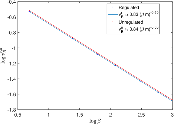
Figure 11: Using the fitted λ0subscript𝜆0\lambda_{0}, λ2subscript𝜆2\lambda_{2} and λisubscript𝜆𝑖\lambda_{i}, the butterfly velocity vBsubscript𝑣𝐵v_{B} is calculated from Eq. 45, and plotted against β𝛽\beta in a log-log scale. The low temperature behavior of vBsubscript𝑣𝐵v_{B} is vB0.83βmsubscript𝑣𝐵0.83𝛽𝑚v_{B}\approx\frac{0.83}{\sqrt{\beta m}} - for both the regulated and the unregulated cases.

For small u𝑢u, the eigenvalues of this matrix equation can be approximated by

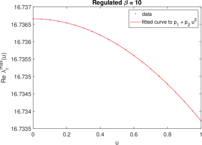
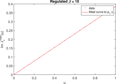
λ~L(u)λ~0λ~2u2±iλ~iu,subscript~𝜆𝐿𝑢plus-or-minussubscript~𝜆0subscript~𝜆2superscript𝑢2𝑖subscript~𝜆𝑖𝑢\tilde{\lambda}_{L}(u)\approx\tilde{\lambda}_{0}-\tilde{\lambda}_{2}u^{2}\pm i\tilde{\lambda}_{i}u, (41)

because of the spherical symmetry of the leading eigenvector at 𝐤=0𝐤0\mathbf{k}=0. Here, λ~0,2,i𝒪(1)similar-tosubscript~𝜆02𝑖𝒪1\tilde{\lambda}_{0,2,i}\sim\mathcal{O}(1), and by rescaling back, λ0,2,ieβm/βNsimilar-tosubscript𝜆02𝑖superscript𝑒𝛽𝑚𝛽𝑁\lambda_{0,2,i}\sim e^{-\beta m}/\beta N. The quadratic form of the real part and the linear form for the imaginary part have been verified numerically in Fig. 20 in App. H. Now, the regulated and unregulated squared commutator can be evaluated as,

Cr,u(t,𝐱)=1Nν𝐤𝐩ei𝐤.𝐱iνt(f+r,u(ν,𝐤;𝐩)2ϵ𝐩+fr,u(ν,𝐤;𝐩)2ϵ𝐩)=1N𝐤ei𝐤.𝐱+λ0tλ2u2t(eiλiutχ𝐤r,u,++eiλiutχ𝐤r,u,),subscript𝐶𝑟𝑢𝑡𝐱1𝑁subscript𝜈subscript𝐤subscript𝐩superscript𝑒formulae-sequence𝑖𝐤𝐱𝑖𝜈𝑡subscriptsuperscript𝑓𝑟𝑢𝜈𝐤𝐩2subscriptitalic-ϵ𝐩subscriptsuperscript𝑓𝑟𝑢𝜈𝐤𝐩2subscriptitalic-ϵ𝐩1𝑁subscript𝐤superscript𝑒formulae-sequence𝑖𝐤𝐱subscript𝜆0𝑡subscript𝜆2superscript𝑢2𝑡superscript𝑒𝑖subscript𝜆𝑖𝑢𝑡subscriptsuperscript𝜒𝑟𝑢𝐤superscript𝑒𝑖subscript𝜆𝑖𝑢𝑡subscriptsuperscript𝜒𝑟𝑢𝐤\begin{split}C_{r,u}(t,\mathbf{x})&=\frac{1}{N}\int_{\nu}\int_{\mathbf{k}}\int_{\mathbf{p}}e^{i\mathbf{k}.\mathbf{x}-i\nu t}\left(\frac{f^{r,u}_{+}(\nu,\mathbf{k};\mathbf{p})}{2\epsilon_{\mathbf{p}}}+\frac{f^{r,u}_{-}(\nu,\mathbf{k};\mathbf{p})}{2\epsilon_{\mathbf{p}}}\right)\\ &=\frac{1}{N}\int_{\mathbf{k}}e^{i\mathbf{k}.\mathbf{x}+\lambda_{0}t-\lambda_{2}u^{2}t}\left(e^{i\lambda_{i}ut}\chi^{r,u,+}_{\mathbf{k}}+e^{-i\lambda_{i}ut}\chi^{r,u,-}_{\mathbf{k}}\right),\end{split} (42)

where, χ𝐤r,u,±subscriptsuperscript𝜒𝑟𝑢plus-or-minus𝐤\chi^{r,u,\pm}_{\mathbf{k}} is the eigenvector of the matrix eigenvalue in Eq. 38. If there are no singularities in χ𝐤r,u,±subscriptsuperscript𝜒𝑟𝑢plus-or-minus𝐤\chi^{r,u,\pm}_{\mathbf{k}}, we can assume the two terms in the integral depends only on the saddle points of the exponents. Recalling u=k/(βmΓ0)𝑢𝑘𝛽𝑚subscriptΓ0u=k/\left(\sqrt{\beta m}\Gamma_{0}\right), the two saddle points are given by,

𝐤±=(βmΓo2)i(𝐱±λitβmΓ0)2λ2t.subscriptsuperscript𝐤plus-or-minus𝛽𝑚superscriptsubscriptΓ𝑜2𝑖plus-or-minus𝐱subscript𝜆𝑖𝑡𝛽𝑚subscriptΓ02subscript𝜆2𝑡\mathbf{k}^{*}_{\pm}=(\beta m\Gamma_{o}^{2})\frac{i\left(\mathbf{x}\pm\frac{\lambda_{i}t}{\sqrt{\beta m}\Gamma_{0}}\right)}{2\lambda_{2}t}. (43)

When Cr,u(t,𝐱)subscript𝐶𝑟𝑢𝑡𝐱C_{r,u}(t,\mathbf{x}) is evaluated, one of the terms will be exponentially suppressed in x𝑥x compared to the other. Keeping only the leading term, we get,

Cr,u(t,𝐱)1Nexp[λ0tβmΓ02(xλitβmΓ0)24λ2t].similar-tosubscript𝐶𝑟𝑢𝑡𝐱1𝑁subscript𝜆0𝑡𝛽𝑚superscriptsubscriptΓ02superscript𝑥subscript𝜆𝑖𝑡𝛽𝑚subscriptΓ024subscript𝜆2𝑡C_{r,u}(t,\mathbf{x})\sim\frac{1}{N}\exp\left[\lambda_{0}t-\frac{\beta m\Gamma_{0}^{2}\left(x-\frac{\lambda_{i}t}{\sqrt{\beta m}\Gamma_{0}}\right)^{2}}{4\lambda_{2}t}\right]. (44)

The first term comes from the pure exponential growth that was present for the u=0𝑢0u=0 case, and the second term is reminiscent of the broadening form of the squared commutator in Eq. 7. By finding the level sets of the exponential for the ballistic condition xvBtsimilar-to𝑥subscript𝑣𝐵𝑡x\sim v_{B}t, we have the following expression for the butterfly velocity vBsubscript𝑣𝐵v_{B},

vBr,u=4λ0λ2βmΓ02+λiβmΓ02.superscriptsubscript𝑣𝐵𝑟𝑢4subscript𝜆0subscript𝜆2𝛽𝑚superscriptsubscriptΓ02subscript𝜆𝑖𝛽𝑚superscriptsubscriptΓ02\begin{split}v_{B}^{r,u}=\sqrt{\frac{4\lambda_{0}\lambda_{2}}{\beta m\Gamma_{0}^{2}}}+\frac{\lambda_{i}}{\sqrt{\beta m\Gamma_{0}^{2}}}.\end{split} (45)

Since λ0,2,iΓ0similar-tosubscript𝜆02𝑖subscriptΓ0\lambda_{0,2,i}\sim\Gamma_{0}, we get the following temperature dependence of the butterfly velocity,

vBr,u1βm.similar-tosuperscriptsubscript𝑣𝐵𝑟𝑢1𝛽𝑚v_{B}^{r,u}\sim\sqrt{\frac{1}{\beta m}}. (46)

Note that this is the same scale as the speed of sound of the ideal classical gas at finite temperature. Hence the butterfly velocity from the regulated squared commutator of this essentially classical gas has the same temperature scaling as the speed of sound. Furthermore, the particular temperature scaling 1/βm1𝛽𝑚\sqrt{1/\beta m} of the butterfly velocity arises because the thermal scale is the appropriate scale to non-dimensionalize the momenta, and doesn’t depend on the exact form of λ~L(u)subscript~𝜆𝐿𝑢\tilde{\lambda}_{L}(u).

From the numerically obtained eigenvalues, we can see from Fig. 11, that the butterfly velocity from regulated and unregulated squared commutators are the same at low temperatures,

vB0.83βm.subscript𝑣𝐵0.83𝛽𝑚v_{B}\approx\frac{0.83}{\sqrt{\beta m}}. (47)

This shows that the ladder calculation is insensitive to contour dependence.

At fixed t𝑡t, for a fixed difference of Cr,u(t,𝐱)subscript𝐶𝑟𝑢𝑡𝐱C_{r,u}(t,\mathbf{x}), one finds from Eq. 44 that the spread ϵ=xvBtitalic-ϵ𝑥subscript𝑣𝐵𝑡similar-toabsent\epsilon=x-v_{B}t\sim constant. This implies that this form of the squared commutator doesn’t have a broadening behavior. A similar exercise for the spin chain result in Eq. 7, would show a time dependent spread, ϵtp/(p+1)similar-toitalic-ϵsuperscript𝑡𝑝𝑝1\epsilon\sim t^{p/(p+1)}, implying broadening.

In deriving these results, we assumed that the integral expression of the squared commutator in Eq. 42 is dominated by the saddle point contribution. In Gu and Kitaev (2019), it was noted that OTOCs obtained from ladder sum calculations generically have a pole in momentum space wherever λL(k)=2π/βsubscript𝜆𝐿𝑘2𝜋𝛽\lambda_{L}(k)=2\pi/\beta,

C(t,𝐱)1N𝐤ei𝐤.𝐱+λL(k)tcosλL(k)β4.similar-to𝐶𝑡𝐱1𝑁subscript𝐤superscript𝑒formulae-sequence𝑖𝐤𝐱subscript𝜆𝐿𝑘𝑡subscript𝜆𝐿𝑘𝛽4C(t,\mathbf{x})\sim\frac{1}{N}\int_{\mathbf{k}}\frac{e^{i\mathbf{k}.\mathbf{x}+\lambda_{L}(k)t}}{\cos\frac{\lambda_{L}(k)\beta}{4}}. (48)

However, in the O(N)𝑂𝑁O(N) theory, the chaos exponent λL(k)1/Nsimilar-tosubscript𝜆𝐿𝑘1𝑁\lambda_{L}(k)\sim 1/N is N𝑁N suppressed, hence these poles occur at parametrically large values of the momentum. Provided that x/t𝑥𝑡x/t is N𝑁N-independent, the saddle point momentum is always closer to the real axis than the pole and hence controls the integral. For example, as we have seen from the k𝑘k dependence of λL(k)subscript𝜆𝐿𝑘\lambda_{L}(k) in Fig. 19 in Appendix. H, if λL(k=i|k|)λ0β|k|2/msimilar-tosubscript𝜆𝐿𝑘𝑖𝑘subscript𝜆0𝛽superscript𝑘2𝑚\lambda_{L}(k=i|k|)\sim\lambda_{0}\beta|k|^{2}/m at large imaginary k𝑘k, then the closest pole in the upper half plane would be at |k|mβNλmaxλ0similar-to𝑘𝑚𝛽𝑁subscript𝜆maxsubscript𝜆0|k|\sim\sqrt{\frac{m}{\beta}\frac{N\lambda_{\text{max}}}{\lambda_{0}}}. This momentum is very large due to large N𝑁N and the large ratio λmax/λ0subscript𝜆maxsubscript𝜆0\lambda_{\text{max}}/\lambda_{0}.

III.3 Summary of findings from the field theory calculation

In this section, we studied the temperature and contour dependence of squared commutator in a solvable large N𝑁N local model using the ladder technique. We find that our analysis can describe the temperature scaling of the butterfly velocity. However, it is insensitive to the contour of thermal ordering. This is not unexpected, as the ladder method is not expected to exhibit contour dependence Kobrin et al. (2020). It also doesn’t capture the broadening behavior that was observed in Sec. II.

The field theory model differs from the spin chain numerics in two ways - the number of spatial dimensions, and in the fact that the spin chain has finite local Hilbert space unlike the field theory model, which is solvable at large N𝑁N - an effectively classical description. It is thus likely that the broadening and the contour dependence are sourced by quantum fluctuations due to the finiteness of the local Hilbert space Xu and Swingle (2019b), which is not captured in this calculation.

IV Discussions

In this paper we have studied the temperature and contour dependence of quantum information scrambling for local gapped interacting systems in two different models and for a wide range of temperatures.

We first introduced a tensor network based technique to calculate both regulated and unregulated squared commutators in quantum spin chains at temperatures ranging across the spectral gap. For the regulated case, the butterfly velocity decreases with lowering temperature, and is consistent with a power law vBβasimilar-tosubscript𝑣𝐵superscript𝛽𝑎v_{B}\sim\beta^{-a} for a>0𝑎0a>0 at intermediate-to-large β𝛽\beta. We also observe a strong contour dependence, and point out that the butterfly velocity obtained from the unregulated squared commutator remains insensitive to the temperature variation. In fact, a careful study of tC(t,𝐱)subscript𝑡𝐶𝑡𝐱\partial_{t}C(t,\mathbf{x}) shows that the chaos bound cannot be generalized away from the special contour ordering used to prove it.

To get an analytical handle on local gapped systems at temperatures lower than what can be accessed in the spin chain numerics, we use a perturbative field theoretic ladder sum technique, and calculate the temperature dependence of the squared commutator in the paramagnetic phase of the O(N)𝑂𝑁O(N) model. There we confirmed that the characteristic speed of information scrambling at low temperature is proportional to the speed of sound of a classical gas, i.e. vBβ1/2similar-tosubscript𝑣𝐵superscript𝛽12v_{B}\sim\beta^{-1/2}, confirming the intuition that the low temperature state can be accurately modeled as a weakly interacting dilute gas of massive quasiparticles. However, the scrambling in this model is insensitive to the contour, and also doesn’t have the broadening feature.

The strong contour dependence we observe in our spin-chain numerics is in the spirit of the results from previous Schwinger-Keldysh calculations in Liao and Galitski (2018); Romero-Bermúdez et al. (2019), which showed similar contour dependence. Our result for the strongly interacting quantum spin chain compliments their perturbative arguments. These results taken together suggest that the unregulated case accesses high energy modes even at low temperatures, thereby remaining insensitive to the effects of temperature. Although we did not find such behavior in the O(N)𝑂𝑁O(N) model at leading order in 1/N1𝑁1/N, we expect higher order corrections will modify this conclusion since there are multiple energy scales in the problem in addition to temperature.

The numerical study also reveals the existence of a wave-front broadening effect that persists even at low temperatures. This feature is not captured in the field theory calculations, and remains an interesting theoretical challenge for the future. As was suggested in Xu and Swingle (2019b), quantum fluctuations due to the finiteness of the local Hilbert spaces will play a significant role in the broadening behavior.

Using Lieb Robinson Lieb and Robinson (1972) bounds, it has recently been demonstrated Han and Hartnoll (2019) that locality and short ranged correlations imply temperature dependent bounds on the butterfly velocity defined from the unregulated squared commutator. In App. I, we review the derivation of this bound and extend it to the regulated case. In particular, it can be shown that the butterfly velocity (obtained from either unregulated or regulated cases) obeys the bound,

βvB0, as β.subscript𝛽subscript𝑣𝐵0, as 𝛽\partial_{\beta}v_{B}\to 0\text{, as }\beta\to\infty. (49)

These bounds are consistent with a constant butterfly velocity at low temperatures vBconstantsimilar-tosubscript𝑣𝐵constantv_{B}\sim\text{constant} (unregulated case from spin chain numerics) and with a butterfly velocity proportional to a power of temperature vBβasimilar-tosubscript𝑣𝐵superscript𝛽𝑎v_{B}\sim\beta^{-a} for a>0𝑎0a>0 (regulated case from the spin chain dynamics and field theory calculation, with a=1/2𝑎12a=1/2). The existing bounds are contour independent and hence cannot constrain the contour dependence.

The strong contour dependence that we observe has non-trivial implications for temperature dependent scrambling studies in future experiments. Our work shows that the regulated and the unregulated cases capture different physics, thus enriching the large set of phenomena falling under the umbrella of scrambling.

V Acknowledgement

The authors would like to thank Shenglong Xu for useful discussions, and Shenglong Xu and Gregory Bentsen for comments on the manuscript. The authors acknowledge the University of Maryland supercomputing resources (http://hpcc.umd.edu) made available for conducting the research reported in this paper. This material is based upon work supported by the Air Force Office of Scientific Research under award number FA9550-17-1-0180.

References

Appendix A Details of MPO numerics

Refer to caption
Refer to caption
Figure 12: We demonstrate the convergence of our numerical method with exact diagonalization for small systems. a) For the regulated case, the χ=8𝜒8\chi=8 result has excellent agreement with exact diagonalization for L=10𝐿10L=10 spin chain at β=1𝛽1\beta=1. b) For the unregulated case, the same agreement is demonstrated for χ=16𝜒16\chi=16 result at β=1𝛽1\beta=1.

We first check the MPO TEBD numerical technique against exact diagonalization. In Fig. 12, we show the comparison of the MPO method to the results of exact diagonalization for a L=10𝐿10L=10 sized spin chain. The machine precision of MATLAB being e36similar-toabsentsuperscript𝑒36\sim e^{-36}, accuracy of logC𝐶\log C from exact diagonalization is 30similar-toabsent30\sim-30. However, in our MPO numerical method, we express the squared commutator as the square of a norm, hence the precision is squared, with reliable numerical data of C𝐶C down to e60similar-toabsentsuperscript𝑒60\sim e^{-60}.

Refer to caption
Refer to caption
Figure 13: a, b) The log of the regulated squared commutator is plotted as a function of time, for the case of an operator X20(t)subscript𝑋20𝑡X_{20}(t) and Zrsubscript𝑍𝑟Z_{r}, with r=30,40,..,200r=30,40,..,200, for bond dimensions χ=4𝜒4\chi=4 (dotted) and χ=8𝜒8\chi=8. The left and the right figures correspond to β=0𝛽0\beta=0 (a) and β=2𝛽2\beta=2 (b) respectively. Even at the low temperature, the data is seen to be converged for the range 50<logCr<3550subscript𝐶𝑟35-50<\log C_{r}<-35. Note we are able to access such small values accurately because we have expressed the regulated squared commutator as a square of a norm, and the norm can be estimated upto the numerical precision of MATLAB which is e36similar-toabsentsuperscript𝑒36\sim e^{-36}, allowing us to push to around e60superscript𝑒60e^{-60} in precision. c, d) The log of the unregulated squared commutator is plotted as a function of time, for the case of an operator X20(t)subscript𝑋20𝑡X_{20}(t) and Zrsubscript𝑍𝑟Z_{r}, with r=30,40,..,200r=30,40,..,200, for bond dimensions χ=8𝜒8\chi=8 (dotted) and χ=16𝜒16\chi=16. The left and the right figures correspond to β=0𝛽0\beta=0 (c) and β=2𝛽2\beta=2 (d) respectively. Even at the low temperature, the data is seen to be converged for the range 50<logCu<1550subscript𝐶𝑢15-50<\log C_{u}<-15.

In order to demonstrate the convergence of the obtained squared commutator with bond dimension, we plot the log of the regulated and unregulated squared commutators as a function of time for different spatial differences in Fig. 13. Even without numerical fitting, it is clear from Fig. 13 that the regulated squared commutator has a strong temperature dependence, while the unregulated squared commutator is much less sensitive to temperature even when the temperature is tuned from β=0𝛽0\beta=0 to β=2>m1𝛽2superscript𝑚1\beta=2>m^{-1}, where the mass is the spectral gap 1.13similar-toabsent1.13\sim 1.13.

It is also seen that the early time data converges well with bond dimension. As has been noted before in Hémery et al. (2019), the qualitative lightcone behavior of the unconverged data obtained from the MPO method can be qualitatively different; hence for all our analysis and fitting we only use numerical data which are shown to converge.

Refer to caption
Figure 14: The collapse of the obtained regulated squared commutator for the data range 50<logCr<3550subscript𝐶𝑟35-50<\log C_{r}<-35, 20<x<20020𝑥20020<x<200 and 20<t<10020𝑡10020<t<100, to the near wave-front ansatz by least squared method. We have chosen this data range as we have confirmed the convergence of our numerical procedure in this range.
Refer to caption
Refer to caption
Figure 15: a) Broadening coefficient p𝑝p obtained from the numerical fitting of regulated squared commutator is plotted as a function of β𝛽\beta. b) p𝑝p from fitting of the unregulated squared commutator is plotted as a function of β𝛽\beta. The errorbars are from the 95% confidence intervals of the fit. To compare the regulated and the unregulated cases we have fixed the y-axis scales to be the same in the two plots.

We fit the converged data using least squared error method to the near wave-front ansatz of Eq. 7. The goodness of fit is studied in Fig. 14, where the data collapse to the fitted model is shown at different temperatures.

The unregulated squared commutator was studied using a similar numerical technique in Han and Hartnoll (2019). Our results indicate that the butterfly velocity obtained from the unregulated squared commutator is constant as function of temperature, even at temperatures lower than the gap, in contradiction with the indicated result from Han and Hartnoll (2019). We checked the case for the [Z(t),Z]𝑍𝑡𝑍[Z(t),Z] type squared commutators as well, and our results are the same for both cases. In Han and Hartnoll (2019), the fitting was done for a much smaller spatio-temporal region 20<x<4520𝑥4520<x<45 and 1<t<51𝑡51<t<5 (in our units), and for a much smaller range logCu>22subscript𝐶𝑢22\log C_{u}>-22, as compared to the situation considered here.

We also study the temperature dependence of the broadening coefficient obtained from the fitting in Fig. 15a (regulated) and Fig. 15b(unregulated). For the unregulated case, we see a fairly constant p𝑝p which is insensitive to decreasing temperature. The regulated case shows an increasing trend with decreasing temperature.

Appendix B Contour dependence and chaos bound

Refer to caption
Refer to caption
Figure 16: a) The data of the unregulated squared commutator for the data range 50<logCu<1550subscript𝐶𝑢15-50<\log C_{u}<-15, is picked out along the ‘ray’ x=t𝑥𝑡x=t. tCusubscript𝑡subscript𝐶𝑢\partial_{t}C_{u} is evaluated in this domain, and the averaged tCusubscript𝑡subscript𝐶𝑢\partial_{t}C_{u} along x=t𝑥𝑡x=t is plotted as a function of β𝛽\beta in b). Similarly data for the unregulated case can be picked up. b) The averaged tCu,rsubscript𝑡subscript𝐶𝑢𝑟\partial_{t}C_{u,r} along x=t𝑥𝑡x=t is plotted as a function of β𝛽\beta.

We analyse in detail the contour dependence of tCu,rsubscript𝑡subscript𝐶𝑢𝑟\partial_{t}C_{u,r}, as was done in Sec. II.4. In Fig. 16, we sketch how tCu,rsubscript𝑡subscript𝐶𝑢𝑟\partial_{t}C_{u,r} is found without numerical fitting. We first pick out data along a ‘ray’ x=t𝑥𝑡x=t, wherever the squared commutator has converged, and study tCu,rsubscript𝑡subscript𝐶𝑢𝑟\partial_{t}C_{u,r} numerically. In Fig. 16b the averaged tlogCu,rsubscript𝑡subscript𝐶𝑢𝑟\partial_{t}\log C_{u,r} along this ray is plotted as a function of β𝛽\beta, and compared against the bound on chaos. The result is similar to Fig. 5, which was obtained by fitting to the near wavefront ansatz. Given the constancy of the unregulated case, the chaos bound could be violated at lower temperatures. These results are for a particular ray x=t𝑥𝑡x=t, and as a function of β𝛽\beta. We can also study tlogCu,rsubscript𝑡subscript𝐶𝑢𝑟\partial_{t}\log C_{u,r} as function of the ray velocity v𝑣v, where x=vt𝑥𝑣𝑡x=vt, for a particular β𝛽\beta. If the near wavefront scrambling ansatz (Eq. 7) is satisfied, then tlogCu,rsubscript𝑡subscript𝐶𝑢𝑟\partial_{t}\log C_{u,r} along a ray of velocity v𝑣v is given by λp(v/vB1)p(1+pv/vB)subscript𝜆𝑝superscript𝑣subscript𝑣𝐵1𝑝1𝑝𝑣subscript𝑣𝐵\lambda_{p}(v/v_{B}-1)^{p}(1+pv/v_{B}). As v𝑣v is increased beyond the vBsubscript𝑣𝐵v_{B}, the near wavefront ansatz predicts that the chaos bound can be violated. We test this numerically in Fig. 17, and we see that indeed tlogCu,r(t,vt)subscript𝑡subscript𝐶𝑢𝑟𝑡𝑣𝑡\partial_{t}\log C_{u,r}(t,vt) deviates from its near ansatz prediction at higher v𝑣v.

Refer to caption
Refer to caption
Figure 17: a) The data of the unregulated squared commutator for the data range 50<logCu<1550subscript𝐶𝑢15-50<\log C_{u}<-15, is picked up along different‘rays’ x=vt𝑥𝑣𝑡x=vt. This procedure can be repeated for the regulated case. b) For different v𝑣v-s, tlogCusubscript𝑡subscript𝐶𝑢\partial_{t}\log C_{u} is plotted as a function of t𝑡t (dots), and compared against the prediction from the near wavefront ansatz (constant lines whose thickness signify the confidence interval from the fitting to the ansatz). For lower v𝑣v (i.e.) closer to the butterfly velocity vBsubscript𝑣𝐵v_{B}, the near wavefront behavior and the numerical result are the same, but they deviate for high ray velocities. The constancy of tlogCusubscript𝑡subscript𝐶𝑢\partial_{t}\log C_{u} along rays allow us to study their time averages as a function of β𝛽\beta.

We also compare tlogCu,r(t,vt)subscript𝑡subscript𝐶𝑢𝑟𝑡𝑣𝑡\partial_{t}\log C_{u,r}(t,vt) against the chaos bound as a function of ray velocity v𝑣v in Fig. 18, and see that for high ray velocities, the bound is violated for both the regulated and unregulated cases. Note however that the analysis on the data is done only on the domain where the data has converged and also lies along the rays - severely restricting the domain on which numerical differentiation can be reliably done to obtain tlogCu,r(t,vt)subscript𝑡subscript𝐶𝑢𝑟𝑡𝑣𝑡\partial_{t}\log C_{u,r}(t,vt).

Refer to caption
Refer to caption
Figure 18: a) Time average of tlogCu(t,vt)subscript𝑡subscript𝐶𝑢𝑡𝑣𝑡\partial_{t}\log C_{u}(t,vt) is plotted for β=1.6𝛽1.6\beta=1.6 as a function of ray velocity v𝑣v (blue dots), and compared against the prediction from the near wavefront ansatz (red dots). b) Same analysis is done for the regulated case. The yellow line in both case refer to the chaos bound at β=1.6𝛽1.6\beta=1.6.

Appendix C Spectral representation and the generalized Wightman function

From the definition of the generalized Wightman function in Eq. 20, we go to the Fourier space, and expand in terms of many body eigenstates |nket𝑛|n\rangle with energy Ensubscript𝐸𝑛E_{n} and momentum Pnsubscript𝑃𝑛P_{n},

𝒢Wα(ω,𝐤)=1(2π)3𝑑teiωtd2xmnn|ραϕ(t,𝐱)|mm|ρ1αϕ(0,𝟎)|n.superscriptsubscript𝒢𝑊𝛼𝜔𝐤1superscript2𝜋3differential-d𝑡superscript𝑒𝑖𝜔𝑡superscript𝑑2𝑥subscript𝑚𝑛quantum-operator-product𝑛superscript𝜌𝛼italic-ϕ𝑡𝐱𝑚quantum-operator-product𝑚superscript𝜌1𝛼italic-ϕ00𝑛\mathcal{G}_{W}^{\alpha}(\omega,\mathbf{k})=\frac{1}{(2\pi)^{3}}\int dte^{i\omega t}\int d^{2}x\sum_{mn}\langle n|\rho^{\alpha}\phi(t,\mathbf{x})|m\rangle\langle m|\rho^{1-\alpha}\phi(0,\mathbf{0})|n\rangle. (50)

In Heisenberg representation, ϕ(t,𝐱)=eiPxeiHtϕ(0,𝟎)eiPxeiHtitalic-ϕ𝑡𝐱superscript𝑒𝑖𝑃𝑥superscript𝑒𝑖𝐻𝑡italic-ϕ00superscript𝑒𝑖𝑃𝑥superscript𝑒𝑖𝐻𝑡\phi(t,\mathbf{x})=e^{-iPx}e^{iHt}\phi(0,\mathbf{0})e^{iPx}e^{-iHt}. This allows us to write the spectral representation of the generalized Wightman function,

𝒢Wα(ω,𝐤)=1Zmn|n|ϕ|m|2δ(ω(EmEn))δ(𝐤(PmPn))eβ(αEn+(1α)Em).superscriptsubscript𝒢𝑊𝛼𝜔𝐤1𝑍subscript𝑚𝑛superscriptquantum-operator-product𝑛italic-ϕ𝑚2𝛿𝜔subscript𝐸𝑚subscript𝐸𝑛𝛿𝐤subscript𝑃𝑚subscript𝑃𝑛superscript𝑒𝛽𝛼subscript𝐸𝑛1𝛼subscript𝐸𝑚\mathcal{G}_{W}^{\alpha}(\omega,\mathbf{k})=\frac{1}{Z}\sum_{mn}|\langle n|\phi|m\rangle|^{2}\delta\left(\omega-(E_{m}-E_{n})\right)\delta\left(\mathbf{k}-(P_{m}-P_{n})\right)e^{-\beta\left(\alpha E_{n}+(1-\alpha)E_{m}\right)}. (51)

The spectral function can be similarly expanded in the spectral representation,

A(ω,𝐤)=1Zmn|n|ϕ|m|2δ(ω(EmEn))δ(𝐤(PmPn))eβEn(1eβω).𝐴𝜔𝐤1𝑍subscript𝑚𝑛superscriptquantum-operator-product𝑛italic-ϕ𝑚2𝛿𝜔subscript𝐸𝑚subscript𝐸𝑛𝛿𝐤subscript𝑃𝑚subscript𝑃𝑛superscript𝑒𝛽subscript𝐸𝑛1superscript𝑒𝛽𝜔A(\omega,\mathbf{k})=\frac{1}{Z}\sum_{mn}|\langle n|\phi|m\rangle|^{2}\delta\left(\omega-(E_{m}-E_{n})\right)\delta\left(\mathbf{k}-(P_{m}-P_{n})\right)e^{-\beta E_{n}}\left(1-e^{-\beta\omega}\right). (52)

Comparing the two spectral representations, we get the following relation,

𝒢Wα(ω,𝐤)=A(ω,𝐤)2sinhβω2e(α12)βω.superscriptsubscript𝒢𝑊𝛼𝜔𝐤𝐴𝜔𝐤2𝛽𝜔2superscript𝑒𝛼12𝛽𝜔\mathcal{G}_{W}^{\alpha}(\omega,\mathbf{k})=\frac{A(\omega,\mathbf{k})}{2\sinh{\frac{\beta\omega}{2}}}e^{\left(\alpha-\frac{1}{2}\right)\beta\omega}. (53)

Appendix D Polarization bubble calculation

T=0

At T=0𝑇0T=0, the polarization bubble can be evaluated exactly, by changing the Matsubara sum to an integral,

ΠT=0(iνn,𝐪)=12𝐤𝐑(ϵ,ϵ)dω2π1(ω+νn)2+(𝐤+𝐪)2+m21ω2+𝐤2+m2.superscriptΠ𝑇0𝑖subscript𝜈𝑛𝐪12subscript𝐤subscript𝐑italic-ϵitalic-ϵ𝑑𝜔2𝜋1superscript𝜔subscript𝜈𝑛2superscript𝐤𝐪2superscript𝑚21superscript𝜔2superscript𝐤2superscript𝑚2\displaystyle\Pi^{T=0}\left(i\nu_{n},\mathbf{q}\right)=\frac{1}{2}\int_{\mathbf{k}}\int_{\mathbf{R}-(-\epsilon,\epsilon)}\frac{d\omega}{2\pi}\frac{1}{\left(\omega+\nu_{n}\right)^{2}+\left(\mathbf{k}+\mathbf{q}\right)^{2}+m^{2}}\frac{1}{\omega^{2}+\mathbf{k}^{2}+m^{2}}. (54)

The retarded Polarization bubble is obtained by analytically continuing to real frequencies, Π(𝐪,iνnν+i0+)Π𝐪𝑖subscript𝜈𝑛𝜈𝑖superscript0\Pi(\mathbf{q},i\nu_{n}\to\nu+i0^{+}). The integral can be exactly evaluated, and we obtain,

ΠRT=0(ν,𝐪)superscriptsubscriptΠ𝑅𝑇0𝜈𝐪\displaystyle\Pi_{R}^{T=0}\left(\nu,\mathbf{q}\right) =18π1𝐪2ν2arctan𝐪2ν22m.absent18𝜋1superscript𝐪2superscript𝜈2superscript𝐪2superscript𝜈22𝑚\displaystyle=\frac{1}{8\pi}\frac{1}{\sqrt{\mathbf{q}^{2}-\nu^{2}}}\arctan{\frac{\sqrt{\mathbf{q}^{2}-\nu^{2}}}{2m}}. (55)

For ν2𝐪2+4m2superscript𝜈2superscript𝐪24superscript𝑚2\nu^{2}\geq\mathbf{q}^{2}+4m^{2},

Im[ΠRT=0(ν+i0+,𝐪,)]=116ν2𝐪2Re[ΠRT=0(ν+i0+,𝐪)]=116πν2𝐪2log(ν2𝐪2+2mν2𝐪22m).\begin{split}Im[\Pi_{R}^{T=0}(\nu+i0^{+},\mathbf{q},)]&=-\frac{1}{16\sqrt{\nu^{2}-\mathbf{q}^{2}}}\\ Re[\Pi_{R}^{T=0}(\nu+i0^{+},\mathbf{q})]&=\frac{1}{16\pi\sqrt{\nu^{2}-\mathbf{q}^{2}}}\log\left(\frac{\sqrt{\nu^{2}-\mathbf{q}^{2}}+2m}{\sqrt{\nu^{2}-\mathbf{q}^{2}}-2m}\right).\end{split} (56)

For ν2<𝐪2+4m2superscript𝜈2superscript𝐪24superscript𝑚2\nu^{2}<\mathbf{q}^{2}+4m^{2},

Im[ΠRT=0(ν+i0+,𝐪)]=0Re[ΠRT=0(ν+i0+,𝐪)]=18π1𝐪2ν2arctan𝐪2ν22.𝐼𝑚delimited-[]superscriptsubscriptΠ𝑅𝑇0𝜈𝑖superscript0𝐪0𝑅𝑒delimited-[]superscriptsubscriptΠ𝑅𝑇0𝜈𝑖superscript0𝐪18𝜋1superscript𝐪2superscript𝜈2superscript𝐪2superscript𝜈22\begin{split}Im[\Pi_{R}^{T=0}(\nu+i0^{+},\mathbf{q})]&=0\\ Re[\Pi_{R}^{T=0}(\nu+i0^{+},\mathbf{q})]&=\frac{1}{8\pi}\frac{1}{\sqrt{\mathbf{q}^{2}-\nu^{2}}}\arctan{\frac{\sqrt{\mathbf{q}^{2}-\nu^{2}}}{2}}.\end{split} (57)

Finite T

Here, we obtain the low temperature correction to the T=0𝑇0T=0 polarization. At finite T, we introduce the function b(z)=(eβz1)1𝑏𝑧superscriptsuperscript𝑒𝛽𝑧11b(z)=(e^{\beta z}-1)^{-1} and the ϕitalic-ϕ\phi polarization bubble can be calculated,

Π(iνn,𝐪)=T2iωn𝐤Λ1(ωn+νn)2+ϵ𝐤+𝐪21ωn2+ϵ𝐤2=12𝐤Λdz2πib(z)1(z+iωn)2ϵ𝐤+𝐪21z2ϵ𝐤2=12𝐤Λ14ϵ𝐤ϵ𝐤+𝐪[b(ϵ𝐤)b(ϵ𝐤+𝐪)ϵ𝐤ϵ𝐤+𝐪+iνnb(ϵ𝐤)+b(ϵ𝐤+𝐪)ϵ𝐤+ϵ𝐤+𝐪+iνnb(ϵ𝐤)+b(ϵ𝐤+𝐪)ϵ𝐤+ϵ𝐤+𝐪iνnb(ϵ𝐤)b(ϵ𝐤+𝐪)ϵ𝐤+𝐪ϵ𝐤+iνn]Π𝑖subscript𝜈𝑛𝐪𝑇2subscript𝑖subscript𝜔𝑛superscriptsubscript𝐤Λ1superscriptsubscript𝜔𝑛subscript𝜈𝑛2superscriptsubscriptitalic-ϵ𝐤𝐪21superscriptsubscript𝜔𝑛2superscriptsubscriptitalic-ϵ𝐤212superscriptsubscript𝐤Λcontour-integral𝑑𝑧2𝜋𝑖𝑏𝑧1superscript𝑧𝑖subscript𝜔𝑛2superscriptsubscriptitalic-ϵ𝐤𝐪21superscript𝑧2superscriptsubscriptitalic-ϵ𝐤212superscriptsubscript𝐤Λ14subscriptitalic-ϵ𝐤subscriptitalic-ϵ𝐤𝐪delimited-[]𝑏subscriptitalic-ϵ𝐤𝑏subscriptitalic-ϵ𝐤𝐪subscriptitalic-ϵ𝐤subscriptitalic-ϵ𝐤𝐪𝑖subscript𝜈𝑛𝑏subscriptitalic-ϵ𝐤𝑏subscriptitalic-ϵ𝐤𝐪subscriptitalic-ϵ𝐤subscriptitalic-ϵ𝐤𝐪𝑖subscript𝜈𝑛𝑏subscriptitalic-ϵ𝐤𝑏subscriptitalic-ϵ𝐤𝐪subscriptitalic-ϵ𝐤subscriptitalic-ϵ𝐤𝐪𝑖subscript𝜈𝑛𝑏subscriptitalic-ϵ𝐤𝑏subscriptitalic-ϵ𝐤𝐪subscriptitalic-ϵ𝐤𝐪subscriptitalic-ϵ𝐤𝑖subscript𝜈𝑛\begin{split}\Pi(i\nu_{n},\mathbf{q})&=\frac{T}{2}\sum_{i\omega_{n}}\int_{\mathbf{k}}^{\Lambda}\frac{1}{(\omega_{n}+\nu_{n})^{2}+\epsilon_{\mathbf{k}+\mathbf{q}}^{2}}\frac{1}{\omega_{n}^{2}+\epsilon_{\mathbf{k}}^{2}}\\ &=\frac{1}{2}\int_{\mathbf{k}}^{\Lambda}\oint\frac{dz}{2\pi i}b(z)\frac{1}{(z+i\omega_{n})^{2}-\epsilon_{\mathbf{k}+\mathbf{q}}^{2}}\frac{1}{z^{2}-\epsilon_{\mathbf{k}}^{2}}\\ &=-\frac{1}{2}\int_{\mathbf{k}}^{\Lambda}\frac{1}{4\epsilon_{\mathbf{k}}\epsilon_{\mathbf{k}+\mathbf{q}}}\left[\frac{b(\epsilon_{\mathbf{k}})-b(\epsilon_{\mathbf{k}+\mathbf{q}})}{\epsilon_{\mathbf{k}}-\epsilon_{\mathbf{k}+\mathbf{q}}+i\nu_{n}}-\frac{b(\epsilon_{\mathbf{k}})+b(\epsilon_{\mathbf{k}+\mathbf{q}})}{\epsilon_{\mathbf{k}}+\epsilon_{\mathbf{k}+\mathbf{q}}+i\nu_{n}}\right.\\ &\left.-\frac{b(-\epsilon_{\mathbf{k}})+b(\epsilon_{\mathbf{k}+\mathbf{q}})}{\epsilon_{\mathbf{k}}+\epsilon_{\mathbf{k}+\mathbf{q}}-i\nu_{n}}-\frac{b(\epsilon_{\mathbf{k}})-b(\epsilon_{\mathbf{k}+\mathbf{q}})}{\epsilon_{\mathbf{k}+\mathbf{q}}-\epsilon_{\mathbf{k}}+i\nu_{n}}\right]\end{split} (58)

Using b(z)=b(z)1𝑏𝑧𝑏𝑧1b(-z)=-b(z)-1 and for our hierarchy of scales, b(ϵ𝐤)eβϵ𝐤<<1𝑏subscriptitalic-ϵ𝐤superscript𝑒𝛽subscriptitalic-ϵ𝐤much-less-than1b(\epsilon_{\mathbf{k}})\approx e^{-\beta\epsilon_{\mathbf{k}}}<<1 for any 𝐤𝐤\mathbf{k}, we can replace b(z)1𝑏𝑧1b(-z)\to-1. The retarded polarization bubble is obtained by analytically continuing from the imaginary Matsubara frequency to real frequency, Π(iνn,𝐪)ΠR(ν+i0+,𝐪)Π𝑖subscript𝜈𝑛𝐪subscriptΠ𝑅𝜈𝑖superscript0𝐪\Pi(i\nu_{n},\mathbf{q})\to\Pi_{R}(\nu+i0^{+},\mathbf{q}). Using Cauchy imaginary value theorem, the imaginary part can be obtained to be (restricting to ν>0𝜈0\nu>0)

Im[ΠR(ν+i0+,𝐪)]=12𝐤Λπ4ϵ𝐤ϵ𝐤+𝐪[δ(ϵ𝐤+ϵ𝐤+𝐪ν)+2(eβϵ𝐤+𝐪eβϵ𝐤)δ(ϵ𝐤+𝐪ϵ𝐤+ν)].𝐼𝑚delimited-[]subscriptΠ𝑅𝜈𝑖superscript0𝐪12superscriptsubscript𝐤Λ𝜋4subscriptitalic-ϵ𝐤subscriptitalic-ϵ𝐤𝐪delimited-[]𝛿subscriptitalic-ϵ𝐤subscriptitalic-ϵ𝐤𝐪𝜈2superscript𝑒𝛽subscriptitalic-ϵ𝐤𝐪superscript𝑒𝛽subscriptitalic-ϵ𝐤𝛿subscriptitalic-ϵ𝐤𝐪subscriptitalic-ϵ𝐤𝜈Im[\Pi_{R}(\nu+i0^{+},\mathbf{q})]=\frac{1}{2}\int_{\mathbf{k}}^{\Lambda}\frac{\pi}{4\epsilon_{\mathbf{k}}\epsilon_{\mathbf{k}+\mathbf{q}}}\left[\delta(\epsilon_{\mathbf{k}}+\epsilon_{\mathbf{k}+\mathbf{q}}-\nu)+2\left(e^{-\beta\epsilon_{\mathbf{k}+\mathbf{q}}}-e^{-\beta\epsilon_{\mathbf{k}}}\right)\delta(\epsilon_{\mathbf{k}+\mathbf{q}}-\epsilon_{\mathbf{k}}+\nu)\right]. (59)

The first term is the T=0𝑇0T=0 result, which was also obtained in the previous paragraph. At finite T𝑇T, the only modification is the second term, which we now evaluate.

In order to evaluate this integral, we need to impose the delta function condition. First we shift the 𝐤𝐤\mathbf{k} integral to 𝐤+𝐪/2𝐤𝐪2\mathbf{k}+\mathbf{q}/2. We also change notation ϵ±=ϵ𝐤±𝐪/2subscriptitalic-ϵplus-or-minussubscriptitalic-ϵplus-or-minus𝐤𝐪2\epsilon_{\pm}=\epsilon_{\mathbf{k}\pm\mathbf{q}/2}. The delta function conditions are then, ϵ++sϵ=sνsubscriptitalic-ϵ𝑠subscriptitalic-ϵ𝑠𝜈\epsilon_{+}+s\epsilon_{-}=s\nu, for s=1𝑠1s=-1. Imposing the delta function condition, we get, k=ν2ν2q24m2ν2q2cos2θsuperscript𝑘𝜈2superscript𝜈2superscript𝑞24superscript𝑚2superscript𝜈2superscript𝑞2superscript2𝜃k^{*}=\frac{\nu}{2}\sqrt{\frac{\nu^{2}-q^{2}-4m^{2}}{\nu^{2}-q^{2}\cos^{2}\theta}}, and ϵ±=ν/2kqcosθ/νsubscriptsuperscriptitalic-ϵplus-or-minusminus-or-plus𝜈2superscript𝑘𝑞𝜃𝜈\epsilon^{*}_{\pm}=\mp\nu/2-k^{*}q\cos\theta/\nu. For this to be consistent with the positivity of ϵ±subscriptitalic-ϵplus-or-minus\epsilon_{\pm}, θ(πcos1ν/q,π+cos1ν/q)𝜃𝜋superscript1𝜈𝑞𝜋superscript1𝜈𝑞\theta\in\left(\pi-\cos^{-1}\nu/q,\pi+\cos^{-1}\nu/q\right).

Now, by change of variable in the delta function,

δ(ν+ϵ+ϵ)𝛿𝜈subscriptitalic-ϵsubscriptitalic-ϵ\displaystyle\delta\left(\nu+\epsilon_{+}-\epsilon_{-}\right) =|f(𝐤)|k=k1δ(kk) where,absentsuperscriptsubscript𝑓𝐤𝑘superscript𝑘1𝛿𝑘superscript𝑘 where,\displaystyle=\left|\nabla f(\mathbf{k})\right|_{k=k^{*}}^{-1}\delta(k-k^{*})\text{ where,}
f(𝐤)𝑓𝐤\displaystyle f(\mathbf{k}) =(𝐤+𝐪/2)2+m2(𝐤𝐪/2)2+m2+ν.absentsuperscript𝐤𝐪22superscript𝑚2superscript𝐤𝐪22superscript𝑚2𝜈\displaystyle=\sqrt{(\mathbf{k}+\mathbf{q}/2)^{2}+m^{2}}-\sqrt{(\mathbf{k}-\mathbf{q}/2)^{2}+m^{2}}+\nu.

We then do the radial k𝑘k integral, by setting kk𝑘superscript𝑘k\to k^{*}. In order to do the θ𝜃\theta integral, we can employ the Laplace method, as the integrand has the exponential factor, eβqcosθq2ν2+4m22q2cos2θν2superscript𝑒𝛽𝑞𝜃superscript𝑞2superscript𝜈24superscript𝑚22superscript𝑞2superscript2𝜃superscript𝜈2e^{\frac{\beta q\cos\theta\sqrt{q^{2}-\nu^{2}+4m^{2}}}{2\sqrt{q^{2}\cos^{2}\theta-\nu^{2}}}}, and βm>>1much-greater-than𝛽𝑚1\beta m>>1. The exponent has a maxima at θ=π𝜃𝜋\theta=\pi, which lies in the allowed domain of θ𝜃\theta. Doing the integral, we get the full correction, for ν<q𝜈𝑞\nu<q,

ImΠR(ν,𝐪)=18π4πβsinh(βν2)(1q2(4m2ν2+q2)(q2ν2))1/4eβq24m2ν2+q2q2ν2𝐼𝑚subscriptΠ𝑅𝜈𝐪18𝜋4𝜋𝛽𝛽𝜈2superscript1superscript𝑞24superscript𝑚2superscript𝜈2superscript𝑞2superscript𝑞2superscript𝜈214superscript𝑒βq24superscript𝑚2superscript𝜈2superscript𝑞2superscript𝑞2superscript𝜈2Im\Pi_{R}(\nu,\mathbf{q})=\frac{1}{8\pi}\sqrt{\frac{4\pi}{\beta}}\sinh\left(\frac{\beta\nu}{2}\right)\left(\frac{1}{q^{2}\left(4m^{2}-\nu^{2}+q^{2}\right)\left(q^{2}-\nu^{2}\right)}\right)^{1/4}e^{-\frac{\text{$\beta$q}}{2}\sqrt{\frac{4m^{2}-\nu^{2}+q^{2}}{q^{2}-\nu^{2}}}} (60)

Appendix E Self Energy calculation

To study the temperature dependent relaxation time of the bosonic quasiparticles, we need to evaluate the self energy of ϕitalic-ϕ\phi. The relevant diagrams are shown in Fig. 8. The imaginary part of the self energy has contribution only from the first diagram in Fig. 8, and can be evaluated to give,

Im[ΣR(ω+i0+,𝐪)]=1N𝐤sinhβω/24ϵ𝐤sinhβϵ𝐤/2×[Im[ΠR1(ϵkω,𝐤𝐪)]sinh[β(ϵkω)/2]+Im[ΠR1(ϵkω,𝐤𝐪)]sinh[β(ϵk+ω)/2]].𝐼𝑚delimited-[]subscriptΣ𝑅𝜔𝑖superscript0𝐪1𝑁subscript𝐤𝛽𝜔24subscriptitalic-ϵ𝐤𝛽subscriptitalic-ϵ𝐤2delimited-[]𝐼𝑚delimited-[]superscriptsubscriptΠ𝑅1subscriptitalic-ϵ𝑘𝜔𝐤𝐪𝛽subscriptitalic-ϵ𝑘𝜔2𝐼𝑚delimited-[]superscriptsubscriptΠ𝑅1subscriptitalic-ϵ𝑘𝜔𝐤𝐪𝛽subscriptitalic-ϵ𝑘𝜔2\begin{split}Im[\Sigma_{R}(\omega+i0^{+},\mathbf{q})]&=-\frac{1}{N}\int_{\mathbf{k}}\frac{\sinh{\beta\omega/2}}{4\epsilon_{\mathbf{k}}\sinh{\beta\epsilon_{\mathbf{k}}/2}}\times\\ &\left[\frac{Im[\Pi_{R}^{-1}(\epsilon_{k}-\omega,\mathbf{k}-\mathbf{q})]}{\sinh[\beta(\epsilon_{k}-\omega)/2]}+\frac{Im[\Pi_{R}^{-1}(-\epsilon_{k}-\omega,\mathbf{k}-\mathbf{q})]}{\sinh[-\beta(\epsilon_{k}+\omega)/2]}\right].\end{split} (61)

Note, at low temperature, the second term in the imaginary part of the self-energy can be ignored. Recalling the definition of the Wightman function, we have,

Im[ΣR(ω+i0+,𝐪)]1N𝐤sinhβω/24ϵ𝐤sinhβϵ𝐤/2GW,λ(1/2)(ϵkω,𝐤𝐪).𝐼𝑚delimited-[]subscriptΣ𝑅𝜔𝑖superscript0𝐪1𝑁subscript𝐤𝛽𝜔24subscriptitalic-ϵ𝐤𝛽subscriptitalic-ϵ𝐤2superscriptsubscript𝐺𝑊𝜆12subscriptitalic-ϵ𝑘𝜔𝐤𝐪Im[\Sigma_{R}(\omega+i0^{+},\mathbf{q})]\approx\frac{1}{N}\int_{\mathbf{k}}\frac{\sinh{\beta\omega/2}}{4\epsilon_{\mathbf{k}}\sinh{\beta\epsilon_{\mathbf{k}}/2}}G_{W,\lambda}^{(1/2)}\left(\epsilon_{k}-\omega,\mathbf{k}-\mathbf{q}\right). (62)

The inverse lifetime, or the relaxation rate of ϕitalic-ϕ\phi can be written in terms of the imaginary part of the self energy,

Γ𝐪=Im[ΣR(ϵ𝐪,𝐪)]2ϵq=12N𝐤Λsinh(βϵ𝐪/2)sinh(βϵ𝐤/2)1+(1/2)(𝐤,𝐪), where we have defined,1+(1/2)(𝐤,𝐪)=GW,λ(1/2)(ϵkϵq,𝐤𝐪)4ϵkϵq.subscriptΓ𝐪𝐼𝑚delimited-[]subscriptΣ𝑅subscriptitalic-ϵ𝐪𝐪2subscriptitalic-ϵ𝑞12𝑁superscriptsubscript𝐤Λ𝛽subscriptitalic-ϵ𝐪2𝛽subscriptitalic-ϵ𝐤2subscriptsuperscript12limit-from1𝐤𝐪, where we have defined,subscriptsuperscript12limit-from1𝐤𝐪superscriptsubscript𝐺𝑊𝜆12subscriptitalic-ϵ𝑘subscriptitalic-ϵ𝑞𝐤𝐪4subscriptitalic-ϵ𝑘subscriptitalic-ϵ𝑞\begin{split}\Gamma_{\mathbf{q}}=\frac{Im[\Sigma_{R}(\epsilon_{\mathbf{q}},\mathbf{q})]}{2\epsilon_{q}}&=\frac{1}{2N}\int_{\mathbf{k}}^{\Lambda}\frac{\sinh\left(\beta\epsilon_{\mathbf{q}}/2\right)}{\sinh\left(\beta\epsilon_{\mathbf{k}}/2\right)}\mathcal{R}^{(1/2)}_{1+}(\mathbf{k},\mathbf{q})\text{, where we have defined,}\\ \mathcal{R}^{(1/2)}_{1+}(\mathbf{k},\mathbf{q})&=\frac{G_{W,\lambda}^{(1/2)}\left(\epsilon_{k}-\epsilon_{q},\mathbf{k}-\mathbf{q}\right)}{4\epsilon_{k}\epsilon_{q}}.\end{split} (63)

Note, |ϵkϵq|<|𝐤𝐪|subscriptitalic-ϵ𝑘subscriptitalic-ϵ𝑞𝐤𝐪|\epsilon_{k}-\epsilon_{q}|<|\mathbf{k}-\mathbf{q}|. The Wightman function 𝒢W,λ(1/2)(ϵkϵq,𝐤𝐪)superscriptsubscript𝒢𝑊𝜆12subscriptitalic-ϵ𝑘subscriptitalic-ϵ𝑞𝐤𝐪\mathcal{G}_{W,\lambda}^{(1/2)}(\epsilon_{k}-\epsilon_{q},\mathbf{k}-\mathbf{q}) can be expressed as

Im[𝒢R((ϵkϵq,𝐤𝐪)]sinhβ(ϵ𝐤ϵ𝐪)/2,\frac{-Im[\mathcal{G}_{R}((\epsilon_{k}-\epsilon_{q},\mathbf{k}-\mathbf{q})]}{\sinh{\beta(\epsilon_{\mathbf{k}}-\epsilon_{\mathbf{q}})/2}},

where, Im[𝒢R]𝐼𝑚delimited-[]subscript𝒢𝑅Im[\mathcal{G}_{R}] is given by Im[ΠR1]=Im[ΠR]Re[ΠR]2+Im[ΠR]2𝐼𝑚delimited-[]superscriptsubscriptΠ𝑅1𝐼𝑚delimited-[]subscriptΠ𝑅𝑅𝑒superscriptdelimited-[]subscriptΠ𝑅2𝐼𝑚superscriptdelimited-[]subscriptΠ𝑅2Im[\Pi_{R}^{-1}]=-\frac{Im[\Pi_{R}]}{Re[\Pi_{R}]^{2}+Im[\Pi_{R}]^{2}}. From the calculations in Sec. D, one can read off the expression for Im[ΠR]𝐼𝑚delimited-[]subscriptΠ𝑅Im[\Pi_{R}] which is exponentially suppressed in βm𝛽𝑚\beta m. In the denominator, any temperature dependence can be ignored, because of the leading T=0𝑇0T=0 behavior of Re[ΠR]𝑅𝑒delimited-[]subscriptΠ𝑅Re[\Pi_{R}]. Thus, we have the following approximation for 1(𝐤,𝐪)subscript1𝐤𝐪\mathcal{R}_{1}(\mathbf{k},\mathbf{q}),

1+(1/2)(𝐤,𝐪)18π4πβm14ϵ𝐤ϵ𝐪exp(β|𝐤𝐪|(𝐤𝐪)2(ϵ𝐤ϵ𝐪)2+4m22(𝐤𝐪)2(ϵ𝐤ϵ𝐪)2)×((|𝐤𝐪|2(ϵ𝐤ϵ𝐪)2)3/4|𝐤𝐪|1/2(4m2(ϵ𝐤ϵ𝐪)2+|𝐤𝐪|2)1/4)64π2arctan2(|𝐤𝐪|2(ϵ𝐤ϵ𝐪)2)2.subscriptsuperscript12limit-from1𝐤𝐪18𝜋4𝜋𝛽𝑚14subscriptitalic-ϵ𝐤subscriptitalic-ϵ𝐪𝛽𝐤𝐪superscript𝐤𝐪2superscriptsubscriptitalic-ϵ𝐤subscriptitalic-ϵ𝐪24superscript𝑚22superscript𝐤𝐪2superscriptsubscriptitalic-ϵ𝐤subscriptitalic-ϵ𝐪2superscriptsuperscript𝐤𝐪2superscriptsubscriptitalic-ϵ𝐤subscriptitalic-ϵ𝐪234superscript𝐤𝐪12superscript4superscript𝑚2superscriptsubscriptitalic-ϵ𝐤subscriptitalic-ϵ𝐪2superscript𝐤𝐪21464superscript𝜋2superscript2superscript𝐤𝐪2superscriptsubscriptitalic-ϵ𝐤subscriptitalic-ϵ𝐪22\begin{split}\mathcal{R}^{(1/2)}_{1+}(\mathbf{k},\mathbf{q})\approx\frac{1}{8\pi}\sqrt{\frac{4\pi}{\beta m}}\frac{1}{4\epsilon_{\mathbf{k}}\epsilon_{\mathbf{q}}}\exp\left(-\frac{\beta|\mathbf{k}-\mathbf{q}|\sqrt{(\mathbf{k}-\mathbf{q})^{2}-\left(\epsilon_{\mathbf{k}}-\epsilon_{\mathbf{q}}\right)^{2}+4m^{2}}}{2\sqrt{(\mathbf{k}-\mathbf{q})^{2}-\left(\epsilon_{\mathbf{k}}-\epsilon_{\mathbf{q}}\right)^{2}}}\right)\times\\ \left(\frac{\left(\left|\mathbf{k}-\mathbf{q}\right|^{2}-(\epsilon_{\mathbf{k}}-\epsilon_{\mathbf{q}})^{2}\right)^{3/4}}{\left|\mathbf{k}-\mathbf{q}\right|^{1/2}\left(4m^{2}-(\epsilon_{\mathbf{k}}-\epsilon_{\mathbf{q}})^{2}+\left|\mathbf{k}-\mathbf{q}\right|^{2}\right)^{1/4}}\right)\frac{64\pi^{2}}{\arctan^{2}\frac{\sqrt{\left(\left|\mathbf{k}-\mathbf{q}\right|^{2}-(\epsilon_{\mathbf{k}}-\epsilon_{\mathbf{q}})^{2}\right)}}{2}}.\end{split} (64)

At low temperature, the relaxation rate can be approximated by the Laplace method, since the integrand has a factor exponential in βm𝛽𝑚\beta m (arising from both the prefactor sinh\sinh and 1subscript1\mathcal{R}_{1} functions in Eq. 63).

We define the phase coherence inverse time scale as, τϕ1=Γ𝐪=𝟎superscriptsubscript𝜏italic-ϕ1subscriptΓ𝐪0\tau_{\phi}^{-1}=\Gamma_{\mathbf{q}=\mathbf{0}} Chubukov et al. (1994), which can be evaluated,

Γ0=1τϕ2πNβeβm.subscriptΓ01subscript𝜏italic-ϕ2𝜋𝑁𝛽superscript𝑒𝛽𝑚\displaystyle\Gamma_{0}=\frac{1}{\tau_{\phi}}\approx\frac{2\pi}{N\beta}e^{-\beta m}. (65)

The momentum dependent Γ𝐪subscriptΓ𝐪\Gamma_{\mathbf{q}} can be evaluated numerically,

Γ𝐪12Neβϵ𝐪/2𝐤eβϵ𝐤/21+(1/2)(𝐤,𝐪).subscriptΓ𝐪12𝑁superscript𝑒𝛽subscriptitalic-ϵ𝐪2subscript𝐤superscript𝑒𝛽subscriptitalic-ϵ𝐤2subscriptsuperscript12limit-from1𝐤𝐪\Gamma_{\mathbf{q}}\approx\frac{1}{2N}e^{\beta\epsilon_{\mathbf{q}}/2}\int_{\mathbf{k}}e^{-\beta\epsilon_{\mathbf{k}}/2}\mathcal{R}^{(1/2)}_{1+}(\mathbf{k},\mathbf{q}). (66)

Appendix F Ladder calculation in different contours

The ladder calculation sets up a diagrammatic calculation of the squared commutator in terms of retarded Green functions and Wightman functions of the fields ϕitalic-ϕ\phi and λ𝜆\lambda. Here we give a sketch of how it works, following Chowdhury and Swingle (2017), while also extending their results to the unregulated squared commutator.

Consider the generalized squared commutator,

C(α)(t,𝐱)=1N2abTr(ρα[ϕa,0(t,𝐱),ϕb,0(0,𝟎)]ρ(1α)[ϕa,0(t,𝐱),ϕb,0(0,𝟎)]).subscript𝐶𝛼𝑡𝐱1superscript𝑁2subscript𝑎𝑏𝑇𝑟superscript𝜌𝛼subscriptitalic-ϕ𝑎0𝑡𝐱subscriptitalic-ϕ𝑏000superscript𝜌1𝛼subscriptitalic-ϕ𝑎0𝑡𝐱subscriptitalic-ϕ𝑏000C_{(\alpha)}(t,\mathbf{x})=-\frac{1}{N^{2}}\sum_{ab}Tr\left(\rho^{\alpha}[\phi_{a,0}(t,\mathbf{x}),\phi_{b,0}(0,\mathbf{0})]\rho^{(1-\alpha)}[\phi_{a,0}(t,\mathbf{x}),\phi_{b,0}(0,\mathbf{0})]\right). (67)

To go to the interaction representation for the ϕitalic-ϕ\phi fields, we introduce time evolution operators in the interaction picture,

UI=𝒯exp(i2Na0t𝑑s𝐱λ0(s,𝐱)ϕ02(s,𝐱)),subscript𝑈𝐼𝒯𝑖2𝑁subscript𝑎superscriptsubscript0𝑡differential-d𝑠subscript𝐱subscript𝜆0𝑠𝐱superscriptsubscriptitalic-ϕ02𝑠𝐱U_{I}=\mathcal{T}\exp\left(\frac{i}{2\sqrt{N}}\sum_{a}\int_{0}^{t}ds\int_{\mathbf{x}}\lambda_{0}(s,\mathbf{x})\phi_{0}^{2}(s,\mathbf{x})\right), (68)

where the subscript 00 indicates that the fields time evolve under the non-interacting part of the Hamiltonian. We further drop the factors of N𝑁N and the index structure to obtain,

C(α)(t,𝐱)Tr(ρα[UIϕ0(t,𝐱)UI,ϕ0(0,𝟎)]ρ(1α)[UIϕ0(t,𝐱)UI,ϕ0(0,𝟎)]).similar-tosubscript𝐶𝛼𝑡𝐱𝑇𝑟superscript𝜌𝛼superscriptsubscript𝑈𝐼subscriptitalic-ϕ0𝑡𝐱subscript𝑈𝐼subscriptitalic-ϕ000superscript𝜌1𝛼superscriptsubscript𝑈𝐼subscriptitalic-ϕ0𝑡𝐱subscript𝑈𝐼subscriptitalic-ϕ000C_{(\alpha)}(t,\mathbf{x})\sim-Tr\left(\rho^{\alpha}[U_{I}^{\dagger}\phi_{0}(t,\mathbf{x})U_{I},\phi_{0}(0,\mathbf{0})]\rho^{(1-\alpha)}[U_{I}^{\dagger}\phi_{0}(t,\mathbf{x})U_{I},\phi_{0}(0,\mathbf{0})]\right). (69)

By expanding up to second order of λ𝜆\lambda, we get,

UIϕ0(t)UIϕ0(t)+i20t𝑑s[ϕ0(t),λ0(s)ϕ02(s)]+(i2)20t𝑑s10s1𝑑s2[[ϕ0(t),λ0(s1)ϕ02(s1)],ϕ0(t),λ0(s2)ϕ02(s2)]+,superscriptsubscript𝑈𝐼subscriptitalic-ϕ0𝑡subscript𝑈𝐼subscriptitalic-ϕ0𝑡𝑖2superscriptsubscript0𝑡differential-d𝑠subscriptitalic-ϕ0𝑡subscript𝜆0𝑠superscriptsubscriptitalic-ϕ02𝑠superscript𝑖22superscriptsubscript0𝑡differential-dsubscript𝑠1superscriptsubscript0subscript𝑠1differential-dsubscript𝑠2subscriptitalic-ϕ0𝑡subscript𝜆0subscript𝑠1superscriptsubscriptitalic-ϕ02subscript𝑠1subscriptitalic-ϕ0𝑡subscript𝜆0subscript𝑠2superscriptsubscriptitalic-ϕ02subscript𝑠2\begin{split}U_{I}^{\dagger}\phi_{0}(t)U_{I}\approx\phi_{0}(t)+\frac{i}{2}\int_{0}^{t}ds\left[\phi_{0}(t),\lambda_{0}(s)\phi_{0}^{2}(s)\right]+\\ \left(\frac{i}{2}\right)^{2}\int_{0}^{t}ds_{1}\int_{0}^{s_{1}}ds_{2}\left[\left[\phi_{0}(t),\lambda_{0}(s_{1})\phi_{0}^{2}(s_{1})\right],\phi_{0}(t),\lambda_{0}(s_{2})\phi_{0}^{2}(s_{2})\right]+...,\end{split} (70)

where we have suppressed the spatial dimension.

By combining fields from both ‘sides of the ladder’ in the expanded expression Eq. 69, we get the two distinct types of rungs - the contributions which are called the Type I and Type II rungs in Sec. III.2. The contour dependence appears in the form of the contour dependence of the Wightman functions. For example, the Type I rung is a contour dependent λ𝜆\lambda-Wightman function, Tr(ραλ0(s)ρ1αλ0(s))𝑇𝑟superscript𝜌𝛼subscript𝜆0𝑠superscript𝜌1𝛼subscript𝜆0superscript𝑠Tr\left(\rho^{\alpha}\lambda_{0}(s)\rho^{1-\alpha}\lambda_{0}(s^{\prime})\right), or, 𝒢W,λ(α)(ss)superscriptsubscript𝒢𝑊𝜆𝛼𝑠superscript𝑠\mathcal{G}_{W,\lambda}^{(\alpha)}(s-s^{\prime}). Similarly, for Type II, we get the corresponding contour dependent Wightman functions.

Appendix G Kernel functions at low temperature

G.0.1 1(1/2)subscriptsuperscript121\mathcal{R}^{(1/2)}_{1} kernel

We already calculated the 1+(1/2)subscriptsuperscript12limit-from1\mathcal{R}^{(1/2)}_{1+} kernel in Sec. E, as given in Eq. 64. We now calculate 1(1/2)subscriptsuperscript12limit-from1\mathcal{R}^{(1/2)}_{1-} at low temperatures,

1(1/2)(𝐩,𝐩):=𝒢W,λ(1/2)(ϵ𝐩ϵ𝐩)4ϵ𝐩ϵ𝐩12ϵ𝐩ϵ𝐩eβ(ϵ𝐩+ϵ𝐩)2ImΠRT=0(ϵ𝐩+ϵ𝐩,𝐩𝐩)|ΠR(ϵ𝐩+ϵ𝐩,𝐩𝐩)|2=132ϵ𝐩ϵ𝐩eβ(ϵ𝐩+ϵ𝐩)21(ϵ𝐩+ϵ𝐩)2(𝐩𝐩)21|ΠRT=0(ϵ𝐩+ϵ𝐩,𝐩𝐩)|2.\begin{split}\mathcal{R}^{(1/2)}_{1-}(\mathbf{p^{\prime}},\mathbf{p})&:=\frac{\mathcal{G}^{(1/2)}_{W,\lambda}(-\epsilon_{\mathbf{p}\prime}-\epsilon_{\mathbf{p}})}{4\epsilon_{\mathbf{p}\prime}\epsilon_{\mathbf{p}}}\\ &\approx\frac{1}{2\epsilon_{\mathbf{p}\prime}\epsilon_{\mathbf{p}}}e^{-\frac{\beta(\epsilon_{\mathbf{p}}+\epsilon_{\mathbf{p}\prime})}{2}}\frac{Im\Pi_{R}^{T=0}(\epsilon_{\mathbf{p}\prime}+\epsilon_{\mathbf{p}},\mathbf{p}\prime-\mathbf{p})}{\left|\Pi_{R}(\epsilon_{\mathbf{p}\prime}+\epsilon_{\mathbf{p}},\mathbf{p}\prime-\mathbf{p})\right|^{2}}\\ &=\frac{1}{32\epsilon_{\mathbf{p}\prime}\epsilon_{\mathbf{p}}}e^{-\frac{\beta(\epsilon_{\mathbf{p}}+\epsilon_{\mathbf{p}\prime})}{2}}\frac{1}{\sqrt{(\epsilon_{\mathbf{p}}+\epsilon_{\mathbf{p}\prime})^{2}-(\mathbf{p}\prime-\mathbf{p})^{2}}}\frac{1}{\left|\Pi_{R}^{T=0}(\epsilon_{\mathbf{p}\prime}+\epsilon_{\mathbf{p}},\mathbf{p}\prime-\mathbf{p})\right|^{2}}.\end{split} (71)

1(1/2)(𝐩,𝐩)subscriptsuperscript12limit-from1superscript𝐩𝐩\mathcal{R}^{(1/2)}_{1-}(\mathbf{p^{\prime}},\mathbf{p}) is exponentially suppressed unless p,p<<1much-less-than𝑝superscript𝑝1p,p^{\prime}<<1, while 1+(1/2)(𝐩,𝐩)subscriptsuperscript12limit-from1superscript𝐩𝐩\mathcal{R}^{(1/2)}_{1+}(\mathbf{p^{\prime}},\mathbf{p}) is exponentially suppressed unless |𝐩𝐩|<<1much-less-thansuperscript𝐩𝐩1|\mathbf{p}^{\prime}-\mathbf{p}|<<1. Furthermore, even in the domain where both the exponents are comparable, it can be numerically verified that 1(1/2)(𝐩,𝐩)subscriptsuperscript12limit-from1superscript𝐩𝐩\mathcal{R}^{(1/2)}_{1-}(\mathbf{p^{\prime}},\mathbf{p}) is negligible compared to 1+(1/2)(𝐩,𝐩)subscriptsuperscript12limit-from1superscript𝐩𝐩\mathcal{R}^{(1/2)}_{1+}(\mathbf{p^{\prime}},\mathbf{p}). Hence for the ladder calculation, we ignore 1subscriptlimit-from1\mathcal{R}_{1-}.

G.0.2 2(1/2)subscriptsuperscript122\mathcal{R}^{(1/2)}_{2} kernel

In order to evaluate the 2(1/2)subscriptsuperscript122\mathcal{R}^{(1/2)}_{2} integration, we first need an expression for 𝒢eff(1/2)subscriptsuperscript𝒢12eff\mathcal{G}^{(1/2)}_{\text{eff}} that was defined in Eq. 31. For results correct to the required order of 1/N1𝑁1/N, it is enough to consider 𝒢W(1/2)(ω)𝒬(ω)A(0)(ω)similar-tosubscriptsuperscript𝒢12𝑊𝜔𝒬𝜔superscript𝐴0𝜔\mathcal{G}^{(1/2)}_{W}(\omega)\sim\mathcal{Q}(\omega)A^{(0)}(\omega), where A(0)superscript𝐴0A^{(0)} is the bare ϕitalic-ϕ\phi spectral function, given in Eq. 19. We have also defined the function, 𝒬(ω)=[2sinh(βω/2)]1𝒬𝜔superscriptdelimited-[]2𝛽𝜔21\mathcal{Q}(\omega)=[2\sinh(\beta\omega/2)]^{-1}. Inserting the spectral function in the expression for 𝒢W(1/2)(ω′′ω,𝐩′′𝐩)𝒢W(ωω′′,𝐩𝐩′′)subscriptsuperscript𝒢12𝑊superscript𝜔′′𝜔superscript𝐩′′𝐩subscript𝒢𝑊superscript𝜔superscript𝜔′′superscript𝐩superscript𝐩′′\mathcal{G}^{(1/2)}_{W}(\omega^{\prime\prime}-\omega,\mathbf{p^{\prime\prime}}-\mathbf{p})\mathcal{G}_{W}(\omega^{\prime}-\omega^{\prime\prime},\mathbf{p^{\prime}}-\mathbf{p^{\prime\prime}}) in Eq. 31, allows us to integrate over ω′′superscript𝜔′′\omega^{\prime\prime}. We introduce notation x=𝐩𝐩𝑥superscript𝐩𝐩x=\mathbf{p^{\prime}}-\mathbf{p}, y=𝐩+𝐩2𝑦superscript𝐩𝐩2y=\frac{\mathbf{p^{\prime}}+\mathbf{p}}{2} and ω¯=ωω¯𝜔superscript𝜔𝜔\overline{\omega}=\omega^{\prime}-\omega. We also denote ϵx/2±𝐩′′=:ϵ±\epsilon_{x/2\pm\mathbf{p^{\prime\prime}}}=:\epsilon_{\pm}. We now have the following expression for 𝒢eff(1/2)subscriptsuperscript𝒢12eff\mathcal{G}^{(1/2)}_{\text{eff}},

𝒢eff(1/2)(ω,ω,𝐩,𝐩)=12N𝐩′′πϵ+ϵ(𝒬(ϵ+)𝒬(ω¯ϵ+)𝒢R,λ(ωϵ+,𝐩′′y)𝒢R,λ(ω+ϵ+,𝐩′′+y)[δ(ω¯ϵ+ϵ)δ(ω¯ϵ++ϵ)]𝒬(ϵ+)𝒬(ω¯+ϵ+)𝒢R,λ(ω+ϵ+,𝐩′′y)𝒢R,λ(ωϵ+,𝐩′′+y)[δ(ω¯+ϵ+ϵ)δ(ω¯+ϵ++ϵ)]).subscriptsuperscript𝒢12effsuperscript𝜔𝜔superscript𝐩𝐩12𝑁subscriptsuperscript𝐩′′𝜋subscriptitalic-ϵsubscriptitalic-ϵlimit-from𝒬subscriptitalic-ϵ𝒬¯𝜔subscriptitalic-ϵsubscript𝒢𝑅𝜆𝜔subscriptitalic-ϵsuperscript𝐩′′𝑦subscript𝒢𝑅𝜆𝜔subscriptitalic-ϵsuperscript𝐩′′𝑦delimited-[]𝛿¯𝜔subscriptitalic-ϵsubscriptitalic-ϵ𝛿¯𝜔subscriptitalic-ϵsubscriptitalic-ϵ𝒬subscriptitalic-ϵ𝒬¯𝜔subscriptitalic-ϵsubscript𝒢𝑅𝜆𝜔subscriptitalic-ϵsuperscript𝐩′′𝑦subscript𝒢𝑅𝜆𝜔subscriptitalic-ϵsuperscript𝐩′′𝑦delimited-[]𝛿¯𝜔subscriptitalic-ϵsubscriptitalic-ϵ𝛿¯𝜔subscriptitalic-ϵsubscriptitalic-ϵ\begin{split}\mathcal{G}^{(1/2)}_{\text{eff}}(\omega^{\prime},\omega,\mathbf{p^{\prime}},\mathbf{p})=\frac{1}{2N}\int_{\mathbf{p^{\prime\prime}}}\frac{\pi}{\epsilon_{+}\epsilon_{-}}\bigg{(}\mathcal{Q}(\epsilon_{+})\mathcal{Q}(\overline{\omega}-\epsilon_{+})\mathcal{G}_{R,\lambda}(-\omega-\epsilon_{+},-\mathbf{p^{\prime\prime}}-y)\mathcal{G}_{R,\lambda}(\omega+\epsilon_{+},\mathbf{p^{\prime\prime}}+y)\\ \left[\delta(\overline{\omega}-\epsilon_{+}-\epsilon_{-})-\delta(\overline{\omega}-\epsilon_{+}+\epsilon_{-})\right]\\ -\quad\mathcal{Q}(-\epsilon_{+})\mathcal{Q}(\overline{\omega}+\epsilon_{+})\mathcal{G}_{R,\lambda}(-\omega+\epsilon_{+},-\mathbf{p^{\prime\prime}}-y)\mathcal{G}_{R,\lambda}(\omega-\epsilon_{+},\mathbf{p^{\prime\prime}}+y)\\ \left[\delta(\overline{\omega}+\epsilon_{+}-\epsilon_{-})-\delta(\overline{\omega}+\epsilon_{+}+\epsilon_{-})\right]\bigg{)}.\end{split} (72)

In this expression, because of the delta functions, one can replace the arguments of 𝒬𝒬\mathcal{Q} by ±ϵ±plus-or-minussubscriptitalic-ϵplus-or-minus\pm\epsilon_{\pm}. Note, at low temperature, 𝒬(ϵ±)eβϵ±/2𝒬subscriptitalic-ϵplus-or-minussuperscript𝑒𝛽subscriptitalic-ϵplus-or-minus2\mathcal{Q}(\epsilon_{\pm})\approx e^{-\beta\epsilon_{\pm}/2}, and 𝒬(ϵ±)eβϵ±/2𝒬subscriptitalic-ϵplus-or-minussuperscript𝑒𝛽subscriptitalic-ϵplus-or-minus2\mathcal{Q}(-\epsilon_{\pm})\approx-e^{-\beta\epsilon_{\pm}/2}. We can also use the fact that 𝒢R,λ(ω,𝐪)=𝒢R,λ(ω,𝐪)subscript𝒢𝑅𝜆𝜔𝐪subscript𝒢𝑅𝜆𝜔𝐪\mathcal{G}_{R,\lambda}(\omega,-\mathbf{q})=\mathcal{G}_{R,\lambda}(\omega,\mathbf{q}), and that the real and imaginary parts of 𝒢R,λ(ω,𝐪)subscript𝒢𝑅𝜆𝜔𝐪\mathcal{G}_{R,\lambda}(\omega,\mathbf{q}) are even and odd functions of ω𝜔\omega respectively. This allows for the following simplification,

𝒢R,λ(ω+ϵ+,𝐩′′y)𝒢R,λ(ωϵ+,𝐩′′+y)=1Re[ΠR(ωϵ+,𝐩′′+y)]2+Im[ΠR(ωϵ+,𝐩′′+y)]21|ΠRT=0(ωϵ+,𝐩′′+y)|2.subscript𝒢𝑅𝜆𝜔subscriptitalic-ϵsuperscript𝐩′′𝑦subscript𝒢𝑅𝜆𝜔subscriptitalic-ϵsuperscript𝐩′′𝑦1𝑅𝑒superscriptdelimited-[]subscriptΠ𝑅𝜔subscriptitalic-ϵsuperscript𝐩′′𝑦2𝐼𝑚superscriptdelimited-[]subscriptΠ𝑅𝜔subscriptitalic-ϵsuperscript𝐩′′𝑦21superscriptsuperscriptsubscriptΠ𝑅𝑇0𝜔subscriptitalic-ϵsuperscript𝐩′′𝑦2\begin{split}\mathcal{G}_{R,\lambda}(-\omega+\epsilon_{+},-\mathbf{p^{\prime\prime}}-y)&\mathcal{G}_{R,\lambda}(\omega-\epsilon_{+},\mathbf{p^{\prime\prime}}+y)\\ &=\frac{1}{Re[\Pi_{R}(\omega-\epsilon_{+},\mathbf{p^{\prime\prime}}+y)]^{2}+Im[\Pi_{R}(\omega-\epsilon_{+},\mathbf{p^{\prime\prime}}+y)]^{2}}\\ &\approx\frac{1}{|\Pi_{R}^{T=0}(\omega-\epsilon_{+},\mathbf{p^{\prime\prime}}+y)|^{2}}.\end{split} (73)

We finally arrive at a simple expression for 𝒢eff(1/2)subscriptsuperscript𝒢12eff\mathcal{G}^{(1/2)}_{\text{eff}},

𝒢eff(1/2)(ω,ω,𝐩,𝐩)=12N𝐩′′πeβ(ϵ++ϵ)2ϵ+ϵ(|ΠRT=0(ω+ϵ+,𝐩′′+y)|2[δ(ω¯ϵ+ϵ)+δ(ω¯ϵ++ϵ)]|ΠRT=0(ωϵ+,𝐩′′+y)|2[δ(ω¯+ϵ+ϵ)+δ(ω¯+ϵ++ϵ)]).subscriptsuperscript𝒢12effsuperscript𝜔𝜔superscript𝐩𝐩12𝑁subscriptsuperscript𝐩′′𝜋superscript𝑒𝛽subscriptitalic-ϵsubscriptitalic-ϵ2subscriptitalic-ϵsubscriptitalic-ϵsuperscriptsuperscriptsubscriptΠ𝑅𝑇0𝜔subscriptitalic-ϵsuperscript𝐩′′𝑦2delimited-[]𝛿¯𝜔subscriptitalic-ϵsubscriptitalic-ϵ𝛿¯𝜔subscriptitalic-ϵsubscriptitalic-ϵsuperscriptsuperscriptsubscriptΠ𝑅𝑇0𝜔subscriptitalic-ϵsuperscript𝐩′′𝑦2delimited-[]𝛿¯𝜔subscriptitalic-ϵsubscriptitalic-ϵ𝛿¯𝜔subscriptitalic-ϵsubscriptitalic-ϵ\begin{split}\mathcal{G}^{(1/2)}_{\text{eff}}(\omega^{\prime},\omega,\mathbf{p^{\prime}},\mathbf{p})=\frac{1}{2N}\int_{\mathbf{p^{\prime\prime}}}\frac{\pi e^{-\frac{\beta(\epsilon_{+}+\epsilon_{-})}{2}}}{\epsilon_{+}\epsilon_{-}}\\ \bigg{(}\left|\Pi_{R}^{T=0}(\omega+\epsilon_{+},\mathbf{p^{\prime\prime}}+y)\right|^{-2}\left[\delta(\overline{\omega}-\epsilon_{+}-\epsilon_{-})+\delta(\overline{\omega}-\epsilon_{+}+\epsilon_{-})\right]\\ \left|\Pi_{R}^{T=0}(\omega-\epsilon_{+},\mathbf{p^{\prime\prime}}+y)\right|^{-2}\left[\delta(\overline{\omega}+\epsilon_{+}-\epsilon_{-})+\delta(\overline{\omega}+\epsilon_{+}+\epsilon_{-})\right]\bigg{)}.\end{split} (74)

G.0.3 2+(1/2)subscriptsuperscript12limit-from2\mathcal{R}^{(1/2)}_{2+} kernel

For 2+(1/2)subscriptsuperscript12limit-from2\mathcal{R}^{(1/2)}_{2+}, the relevant function is 𝒢eff(1/2)(ϵ𝐩,ϵ𝐩,𝐩,𝐩)subscriptsuperscript𝒢12effsubscriptitalic-ϵsuperscript𝐩subscriptitalic-ϵ𝐩superscript𝐩𝐩\mathcal{G}^{(1/2)}_{\text{eff}}(\epsilon_{\mathbf{p}^{\prime}},\epsilon_{\mathbf{p}},\mathbf{p}^{\prime},\mathbf{p}), where ω¯=ϵ𝐩ϵ𝐩¯𝜔subscriptitalic-ϵsuperscript𝐩subscriptitalic-ϵ𝐩\overline{\omega}=\epsilon_{\mathbf{p}^{\prime}}-\epsilon_{\mathbf{p}}, and 𝐱=𝐩𝐩𝐱superscript𝐩𝐩\mathbf{x}=\mathbf{p^{\prime}}-\mathbf{p}. The only delta functions in the equation above that can be satisfied are δ(ω¯+ϵ+ϵ)𝛿¯𝜔subscriptitalic-ϵsubscriptitalic-ϵ\delta(\overline{\omega}+\epsilon_{+}-\epsilon_{-}) and δ(ω¯ϵ++ϵ)𝛿¯𝜔subscriptitalic-ϵsubscriptitalic-ϵ\delta(\overline{\omega}-\epsilon_{+}+\epsilon_{-}). We can impose the delta function to do the pp\prime\prime radial integration, which fixes the radial component at p′′(θ)=ω¯2ω¯2x24m2ω¯2x2cos2θsubscriptsuperscript𝑝′′𝜃¯𝜔2superscript¯𝜔2superscript𝑥24superscript𝑚2superscript¯𝜔2superscript𝑥2superscript2𝜃p^{\prime\prime}_{*}(\theta)=\frac{\overline{\omega}}{2}\sqrt{\frac{\overline{\omega}^{2}-x^{2}-4m^{2}}{\overline{\omega}^{2}-x^{2}\cos^{2}{\theta}}}, where θ𝜃\theta is the angle with 𝐱𝐱\mathbf{x}. This can be followed by the angular integration approximated by the Laplace method, since there is an exponential factor with large βm𝛽𝑚\beta m in the exponent. The calculation closely follows the evaluation of ImΠR𝐼𝑚subscriptΠ𝑅Im\Pi_{R} at finite T𝑇T in Appendix D. The final expression for 2+(1/2)subscriptsuperscript12limit-from2\mathcal{R}^{(1/2)}_{2+} is,

2+(1/2)(𝐩,𝐩)18π4πβm14ϵ𝐩ϵ𝐩exp(β|𝐩𝐩|(𝐩𝐩)2(ϵ𝐩ϵ𝐩)2+4m22(𝐩𝐩)2(ϵ𝐩ϵ𝐩)2)×(1|𝐩𝐩|1/2(4m2(ϵ𝐩ϵ𝐩)2+|𝐩𝐩|2)1/4(|𝐩𝐩|2(ϵ𝐩ϵ𝐩)2)1/4)×(|ΠRT=0(ϵ𝐩+ϵ𝐩2xp′′(θ=π)ω¯,𝐩+𝐩2+p′′(θ=π))|2+|ΠRT=0(ϵ𝐩+ϵ𝐩2+xp′′(θ=0)ω¯,𝐩+𝐩2+p′′(θ=0))|2).subscriptsuperscript12limit-from2superscript𝐩𝐩18𝜋4𝜋𝛽𝑚14subscriptitalic-ϵsuperscript𝐩subscriptitalic-ϵ𝐩𝛽superscript𝐩𝐩superscriptsuperscript𝐩𝐩2superscriptsubscriptitalic-ϵsuperscript𝐩subscriptitalic-ϵ𝐩24superscript𝑚22superscriptsuperscript𝐩𝐩2superscriptsubscriptitalic-ϵsuperscript𝐩subscriptitalic-ϵ𝐩21superscriptsuperscript𝐩𝐩12superscript4superscript𝑚2superscriptsubscriptitalic-ϵsuperscript𝐩subscriptitalic-ϵ𝐩2superscriptsuperscript𝐩𝐩214superscriptsuperscriptsuperscript𝐩𝐩2superscriptsubscriptitalic-ϵsuperscript𝐩subscriptitalic-ϵ𝐩214superscriptsuperscriptsubscriptΠ𝑅𝑇0subscriptitalic-ϵsuperscript𝐩subscriptitalic-ϵ𝐩2𝑥subscriptsuperscript𝑝′′𝜃𝜋¯𝜔superscript𝐩𝐩2subscriptsuperscript𝑝′′𝜃𝜋2superscriptsuperscriptsubscriptΠ𝑅𝑇0subscriptitalic-ϵsuperscript𝐩subscriptitalic-ϵ𝐩2𝑥subscriptsuperscript𝑝′′𝜃0¯𝜔superscript𝐩𝐩2subscriptsuperscript𝑝′′𝜃02\begin{split}\mathcal{R}^{(1/2)}_{2+}(\mathbf{p}^{\prime},\mathbf{p})\approx\frac{1}{8\pi}\sqrt{\frac{4\pi}{\beta m}}\frac{1}{4\epsilon_{\mathbf{p}^{\prime}}\epsilon_{\mathbf{p}}}\exp\left(-\frac{\beta|\mathbf{p}^{\prime}-\mathbf{p}|\sqrt{(\mathbf{p}^{\prime}-\mathbf{p})^{2}-\left(\epsilon_{\mathbf{p}^{\prime}}-\epsilon_{\mathbf{p}}\right)^{2}+4m^{2}}}{2\sqrt{(\mathbf{p}^{\prime}-\mathbf{p})^{2}-\left(\epsilon_{\mathbf{p}^{\prime}}-\epsilon_{\mathbf{p}}\right)^{2}}}\right)\times\\ \left(\frac{1}{\left|\mathbf{p}^{\prime}-\mathbf{p}\right|^{1/2}\left(4m^{2}-(\epsilon_{\mathbf{p}^{\prime}}-\epsilon_{\mathbf{p}})^{2}+\left|\mathbf{p}^{\prime}-\mathbf{p}\right|^{2}\right)^{1/4}\left(\left|\mathbf{p}^{\prime}-\mathbf{p}\right|^{2}-(\epsilon_{\mathbf{p}^{\prime}}-\epsilon_{\mathbf{p}})^{2}\right)^{1/4}}\right)\times\\ \left(\left|\Pi_{R}^{T=0}\left(\frac{\epsilon_{\mathbf{p}^{\prime}}+\epsilon_{\mathbf{p}}}{2}-\frac{xp^{\prime\prime}_{*}(\theta=\pi)}{\overline{\omega}},\frac{\mathbf{p}^{\prime}+\mathbf{p}}{2}+p^{\prime\prime}_{*}(\theta=\pi)\right)\right|^{-2}\right.\\ \\ +\left.\left|\Pi_{R}^{T=0}\left(\frac{\epsilon_{\mathbf{p}^{\prime}}+\epsilon_{\mathbf{p}}}{2}+\frac{xp^{\prime\prime}_{*}(\theta=0)}{\overline{\omega}},\frac{\mathbf{p}^{\prime}+\mathbf{p}}{2}+p^{\prime\prime}_{*}(\theta=0)\right)\right|^{-2}\right).\end{split} (75)

G.0.4 2(1/2)subscriptsuperscript12limit-from2\mathcal{R}^{(1/2)}_{2-} kernel

We can similarly evaluate the 2(1/2)subscriptsuperscript12limit-from2\mathcal{R}^{(1/2)}_{2-}, for which the relevant function is 𝒢eff(ϵ𝐩,ϵ𝐩,𝐩,𝐩)subscript𝒢effsubscriptitalic-ϵsuperscript𝐩subscriptitalic-ϵ𝐩superscript𝐩𝐩\mathcal{G}_{\text{eff}}(-\epsilon_{\mathbf{p}^{\prime}},\epsilon_{\mathbf{p}},\mathbf{p}^{\prime},\mathbf{p}). We further define, ω¯=ϵ𝐩+ϵ𝐩¯𝜔subscriptitalic-ϵsuperscript𝐩subscriptitalic-ϵ𝐩\overline{\omega}=\epsilon_{\mathbf{p}^{\prime}}+\epsilon_{\mathbf{p}}, and 𝐱=𝐩𝐩𝐱superscript𝐩𝐩\mathbf{x}=\mathbf{p^{\prime}}-\mathbf{p}. The only delta function in the equation above that can be satisfied is δ(ω¯ϵ+ϵ)𝛿¯𝜔subscriptitalic-ϵsubscriptitalic-ϵ\delta(\overline{\omega}-\epsilon_{+}-\epsilon_{-}). We can impose the delta function to do the pp\prime\prime radial integration, which fixes the radial component at p′′(θ)=ω¯2ω¯2x24m2ω¯2x2cos2θsubscriptsuperscript𝑝′′𝜃¯𝜔2superscript¯𝜔2superscript𝑥24superscript𝑚2superscript¯𝜔2superscript𝑥2superscript2𝜃p^{\prime\prime}_{*}(\theta)=\frac{\overline{\omega}}{2}\sqrt{\frac{\overline{\omega}^{2}-x^{2}-4m^{2}}{\overline{\omega}^{2}-x^{2}\cos^{2}{\theta}}}. This brings an exponential factor of eβ(ϵ𝐩+ϵ𝐩)2superscript𝑒𝛽subscriptitalic-ϵsuperscript𝐩subscriptitalic-ϵ𝐩2e^{-\frac{\beta(\epsilon_{\mathbf{p}^{\prime}}+\epsilon_{\mathbf{p}})}{2}} to the expression for 2(1/2)subscriptsuperscript12limit-from2\mathcal{R}^{(1/2)}_{2-}, and hence 2(1/2)(𝐩,𝐩)subscriptsuperscript12limit-from2superscript𝐩𝐩\mathcal{R}^{(1/2)}_{2-}(\mathbf{p}^{\prime},\mathbf{p}) is substantial only at p,p<<1much-less-than𝑝superscript𝑝1p,p^{\prime}<<1. The approximate expression (after the angular integration) is,

2(1/2)(𝐩,𝐩)18ϵ𝐩ϵ𝐩eβ(ϵ𝐩+ϵ𝐩)2ω¯24m2ω¯2|ΠRT=0(ϵ𝐩ϵ𝐩2,ω¯24m22)|2.subscriptsuperscript12limit-from2superscript𝐩𝐩18subscriptitalic-ϵsuperscript𝐩subscriptitalic-ϵ𝐩superscript𝑒𝛽subscriptitalic-ϵsuperscript𝐩subscriptitalic-ϵ𝐩2superscript¯𝜔24superscript𝑚2superscript¯𝜔2superscriptsuperscriptsubscriptΠ𝑅𝑇0subscriptitalic-ϵ𝐩subscriptitalic-ϵsuperscript𝐩2superscript¯𝜔24superscript𝑚222\begin{split}\mathcal{R}^{(1/2)}_{2-}(\mathbf{p}^{\prime},\mathbf{p})\approx\frac{1}{8\epsilon_{\mathbf{p}^{\prime}}\epsilon_{\mathbf{p}}}e^{-\frac{\beta(\epsilon_{\mathbf{p}^{\prime}}+\epsilon_{\mathbf{p}})}{2}}\frac{\sqrt{\overline{\omega}^{2}-4m^{2}}}{\overline{\omega}^{2}}\left|\Pi_{R}^{T=0}\left(\frac{\epsilon_{\mathbf{p}}-\epsilon_{\mathbf{p}^{\prime}}}{2},\frac{\sqrt{\overline{\omega}^{2}-4m^{2}}}{2}\right)\right|^{-2}.\end{split} (76)

Numerically, it can be verified that 2(1/2)(𝐩,𝐩)subscriptsuperscript12limit-from2superscript𝐩𝐩\mathcal{R}^{(1/2)}_{2-}(\mathbf{p}^{\prime},\mathbf{p}) can always be ignored with respect to 2+(1/2)(𝐩,𝐩)subscriptsuperscript12limit-from2superscript𝐩𝐩\mathcal{R}^{(1/2)}_{2+}(\mathbf{p}^{\prime},\mathbf{p}), for similar reasons as 1subscript1\mathcal{R}_{1}. Hence, for the ladder calculation, we can ignore 2(𝐩,𝐩)subscriptlimit-from2superscript𝐩𝐩\mathcal{R}_{2-}(\mathbf{p}^{\prime},\mathbf{p}).

Appendix H Details of numerics of ladder calculation

Here we provide some details of the numerical computation of the ladder sum. We fix the mass as m=1𝑚1m=1, and do all the calculation in these units. Having determined the approximate values of the kernel functions 1,2subscript12\mathcal{R}_{1,2}, we need to discretize the 2D momentum space to set up the matrix form of the kernel integration. For that purpose, we set up a hard momentum cut-off of |𝐩x|,|𝐩y|1subscript𝐩𝑥subscript𝐩𝑦1|\mathbf{p}_{x}|,|\mathbf{p}_{y}|\leq 1. The choice is justified for the kernel in rescaled momenta, which is exponentially suppressed - exp(|𝐩𝐩|2/8)superscript𝐩superscript𝐩28\exp\left(-|\mathbf{p}-\mathbf{p^{\prime}}|^{2}/8\right). Next, we create 2D grid of momenta, with the momentum interval dp𝑑𝑝dp determined by the number of points that we consider - 40 by 40, 50 by 50 and 60 by 60 grids. Next, we set up the matrix form of the kernel, K^𝐩𝐩=dp2𝒦^(𝐩,𝐩)subscript^𝐾superscript𝐩𝐩𝑑superscript𝑝2^𝒦superscript𝐩𝐩\hat{K}_{\mathbf{p}^{\prime}\mathbf{p}}=dp^{2}\hat{\mathcal{K}}(\mathbf{p}^{\prime},\mathbf{p}), given in Eq. 38. The matrices are of sizes, 1600 by 1600, 2500 by 2500, and 3600 by 3600, respectively. In constructing the matrix, we need to evaluate Γ𝐩subscriptΓ𝐩\Gamma_{\mathbf{p}} by performing a 2D integration (in Eq. 29) within the grid area (|𝐩x|,|𝐩y|1subscript𝐩𝑥subscript𝐩𝑦1|\mathbf{p}_{x}|,|\mathbf{p}_{y}|\leq 1). We find the maximum magnitude eigenvalue of the matrix, and find that the largest magnitude eigenvalue has a positive real part, thereby resulting in exponential growth. The eigenvalues are then extrapolated to the dp0𝑑𝑝0dp\to 0 limit by a linear extrapolation. Errors in the estimation are denoted as the errorbars for this eigenvalue (see Fig. 19).

Refer to caption
Figure 19: The maximum eigenvalue λLeβmβsubscript𝜆𝐿superscript𝑒𝛽𝑚𝛽\lambda_{L}e^{\beta m}\beta is determined by taking the linear extrapolation of λLeβmβsubscript𝜆𝐿superscript𝑒𝛽𝑚𝛽\lambda_{L}e^{\beta m}\beta at each grid interval dp𝑑𝑝dp to dp0𝑑𝑝0dp\to 0. The error is determined as the uncertainty in the extrapolation from its 95%percent9595\% confidence interval. The graph here is shown for the unregulated calculation at β=2𝛽2\beta=2.
Refer to caption
Refer to caption
Figure 20: A sample fit of the numerically obtained λLr(u)superscriptsubscript𝜆𝐿𝑟𝑢\lambda_{L}^{r}(u), at β=10𝛽10\beta=10. m𝑚m is chosen to be 1. The real part is fit to f(u)=λ0λ2u2𝑓𝑢subscript𝜆0subscript𝜆2superscript𝑢2f(u)=\lambda_{0}-\lambda_{2}u^{2}, while the imaginary part is fit to f(u)=λiu𝑓𝑢subscript𝜆𝑖𝑢f(u)=\lambda_{i}u, and the fit works very well even at quite large u.

In Fig. 20, we study the external momentum dependence of the largest magnitude eigenvalue of the kernel equation λL(u)subscript𝜆𝐿𝑢\lambda_{L}(u) at non zero external momentum u𝑢u. The real part of λL(u)subscript𝜆𝐿𝑢\lambda_{L}(u) shows a quadratically decreasing behavior, λ0λ2u2subscript𝜆0subscript𝜆2superscript𝑢2\lambda_{0}-\lambda_{2}u^{2} even at significantly high u𝑢u, while the the imaginary part shows a linear behavior, λiusubscript𝜆𝑖𝑢\lambda_{i}u. At u=0𝑢0u=0, the eigenvalue is real and positive.

Appendix I Bounds on temperature dependence of butterfly velocity
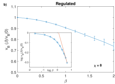
Locality in gapped quantum spin chains can lead to microcausality and short ranged correlation Hastings and Koma (2006). Can we use similar techniques to bound the behavior of butterfly velocity?

In this Appendix we discuss state dependent bounds on butterfly velocity in local gapped systems which were introduced in Han and Hartnoll (2019). The general definition of squared commutator in Eq. 1 can be rewritten as 𝒞α(t,𝐱,ρ)=Tr(ραOρ1αO)subscript𝒞𝛼𝑡𝐱𝜌𝑇𝑟superscript𝜌𝛼𝑂superscript𝜌1𝛼𝑂\mathcal{C}_{\alpha}(t,\mathbf{x},\rho)=-Tr\left(\rho^{\alpha}O\rho^{1-\alpha}O\right), where, O=i[W𝟎(t),V𝐱]𝑂𝑖subscript𝑊0𝑡subscript𝑉𝐱O=i\left[W_{\mathbf{0}}(t),V_{\mathbf{x}}\right]. By restricting to x=vt𝑥𝑣𝑡x=vt, one can define the velocity dependent Lyapunov exponents,

λ(v,ρ)=limt1tlnC(vt,t,ρ).𝜆𝑣𝜌subscript𝑡1𝑡𝐶𝑣𝑡𝑡𝜌\lambda(v,\rho)=\lim_{t\to\infty}\frac{1}{t}\ln C(vt,t,\rho). (77)

The butterfly velocity can be defined as the largest velocity for which the Lyapunov exponent is positive,

vB(ρ)=sup{v:λ(v,ρ)0}.subscript𝑣𝐵𝜌supremumconditional-set𝑣𝜆𝑣𝜌0v_{B}(\rho)=\sup\left\{v:\lambda(v,\rho)\geq 0\right\}. (78)

We define the support of the commutator, O𝑂O as a region S of diameter 2R(v,t)2𝑅𝑣𝑡2R(v,t), around a point 𝟎0\mathbf{0}. The scrambling velocity is defined as the rate of increase of this support,

vS(ρ)=limtR(v,t)t.subscript𝑣𝑆𝜌subscript𝑡𝑅𝑣𝑡𝑡v_{S}(\rho)=\lim_{t\to\infty}\frac{R(v,t)}{t}. (79)

We consider the Hamiltonian H𝐻H to be defined on a lattice, composed of geometrically local terms, and such that it has a finite gap. We introduce the shifted zero expectation-value Hamiltonian, H~=HTr(ρH)~𝐻𝐻𝑇𝑟𝜌𝐻\tilde{H}=H-Tr(\rho H). We can divide the shifted Hamiltonian into terms supported inside and outside S𝑆S,

H~=iSh~i+jΛSh~j.~𝐻subscript𝑖𝑆subscript~𝑖subscript𝑗Λ𝑆subscript~𝑗\tilde{H}=\sum_{i\in S}\tilde{h}_{i}+\sum_{j\in\Lambda-S}\tilde{h}_{j}. (80)

Let us consider the near wavefront ansatz,

λ(v,ρ)=λ(vvB1)1+p.𝜆𝑣𝜌𝜆superscript𝑣subscript𝑣𝐵11𝑝\lambda(v,\rho)=-\lambda\left(\frac{v}{v_{B}}-1\right)^{1+p}. (81)

In Han and Hartnoll (2019), it was shown that for the unregulated squared commutator, the rate of change of butterfly velocity with temperature, βvBsubscript𝛽subscript𝑣𝐵\partial_{\beta}v_{B} can be bounded,

λ(Δv)p(Δv+1)|βlnvB|2h(vS(ρ)ξλ(v,ρ)),𝜆superscriptΔ𝑣𝑝Δ𝑣1subscript𝛽subscript𝑣𝐵2subscript𝑣𝑆𝜌𝜉𝜆𝑣𝜌\lambda(\Delta v)^{p}(\Delta v+1)|\partial_{\beta}\ln v_{B}|\leq 2h\left(v_{S}(\rho)-\xi\lambda(v,\rho)\right), (82)

where Δv=v/vB1Δ𝑣𝑣subscript𝑣𝐵1\Delta v=v/v_{B}-1, ξ>0𝜉0\xi>0 is the finite correlation length, and hh is given by,

h=supi|Tr(ρh~iρOO)|Tr(ρOO).subscriptsup𝑖𝑇𝑟𝜌subscript~𝑖𝜌𝑂𝑂𝑇𝑟𝜌𝑂𝑂h=\text{sup}_{i}\frac{\left|Tr\left(\sqrt{\rho}\tilde{h}_{i}\sqrt{\rho}OO\right)\right|}{Tr\left(\rho OO\right)}. (83)

At low temperature, β𝛽\beta\to\infty, ρ|00|similar-to𝜌ket0bra0\rho\sim|0\rangle\langle 0|. From Eq. 83, h0|h~i|0proportional-toquantum-operator-product0subscript~𝑖0h\propto\langle 0|\tilde{h}_{i}|0\rangle, and hence 0, which implies,

βlnvB0 as β.subscript𝛽subscript𝑣𝐵0 as 𝛽\partial_{\beta}\ln v_{B}\to 0\text{ as }\beta\to\infty. (84)

We first review the proof for the unregulated case due to Han and Hartnoll (2019) and then also extend the bound to the butterfly velocity obtained from the regulated squared commutator, and show that the same low temperature behavior as in Eq. 84 holds in that case as well. However, we note that the bound can’t differentiate between a power-law vanishing butterfly velocity at low temperature and a constant butterfly velocity. Low temperature behaviors of both the regulated and unregulated cases which were obtained in Sec. II, i.e., vBβ1/2similar-tosubscript𝑣𝐵superscript𝛽12v_{B}\sim\beta^{-1/2} and vBconstantsimilar-tosubscript𝑣𝐵constantv_{B}\sim\text{constant} respectively, are consistent with Eq. 84.

We first discuss the bound on butterfly velocity obtained from the unregulated squared commutator as given in Han and Hartnoll (2019). We differentiate Cusubscript𝐶𝑢C_{u} with respect to the inverse temperature β𝛽\beta to obtain,

βCu=Tr(H~ρOO)).\partial_{\beta}C_{u}=-Tr\left(\tilde{H}\rho OO)\right). (85)

We want to upper bound |βCu|subscript𝛽subscript𝐶𝑢|\partial_{\beta}C_{u}|. By separating out the contributing terms to two parts - inside and outside a ball of radius R+δ𝑅𝛿R+\delta around the point x0subscript𝑥0x_{0} (a region we call Ssuperscript𝑆S^{\prime}), we have,

|βCu|iS|Tr(ρOOh~i)|+jΛS|Tr(ρOOh~j)|.subscript𝛽subscript𝐶𝑢subscript𝑖superscript𝑆𝑇𝑟𝜌𝑂𝑂subscript~𝑖subscript𝑗Λsuperscript𝑆𝑇𝑟𝜌𝑂𝑂subscript~𝑗|\partial_{\beta}C_{u}|\leq\sum_{i\in S^{\prime}}\left|Tr\left(\rho OO\tilde{h}_{i}\right)\right|+\sum_{j\in\Lambda-S^{\prime}}\left|Tr\left(\rho OO\tilde{h}_{j}\right)\right|. (86)

For the terms outside the ball Ssuperscript𝑆S^{\prime}, we invoke the Exponential Clustering Theorem, which states, for two operators W1subscript𝑊1W_{1} and W2subscript𝑊2W_{2} supported on non-overlapping regions A𝐴A and B𝐵B on a lattice system with a gapped Hamiltonian, there exist, ξ𝜉\xi and 𝒩𝒩\mathcal{N}, such that,

|Tr(ρW1W2)Tr(ρW1)Tr(ρW2)|𝒩min{|A|,|B|}W1W2e|AB|/ξ,𝑇𝑟𝜌subscript𝑊1subscript𝑊2𝑇𝑟𝜌subscript𝑊1𝑇𝑟𝜌subscript𝑊2𝒩𝑚𝑖𝑛𝐴𝐵delimited-∥∥subscript𝑊1delimited-∥∥subscript𝑊2superscript𝑒𝐴𝐵𝜉\left|Tr\left(\rho W_{1}W_{2}\right)-Tr\left(\rho W_{1}\right)Tr\left(\rho W_{2}\right)\right|\leq\mathcal{N}min\{|\partial A|,|\partial B|\}\lVert W_{1}\rVert\lVert W_{2}\rVert e^{-|A-B|/\xi}, (87)

where, |AB|𝐴𝐵|A-B| is the minimum distance between the regions A𝐴A and B𝐵B. Here, ξ𝜉\xi is the correlation length, which is finite because of the presence of the gap. The Exponential Clustering Theorem can be proved using Lieb Robinson bound techniques Hastings and Koma (2006). Now, Tr(ρh~i)=0𝑇𝑟𝜌subscript~𝑖0Tr\left(\rho\tilde{h}_{i}\right)=0. Thus the sum of ‘outside’ terms in the RHS of Eq. 86, can bounded in the following way -

j2𝒩min{|A|,|B|}O2j=δej/ξ=δ𝑑xex/ξ where  is suitably defined,=ξeδ/ξ.subscript𝑗2𝒩𝑚𝑖𝑛𝐴𝐵superscriptdelimited-∥∥𝑂2superscriptsubscript𝑗𝛿superscript𝑒𝑗𝜉superscriptsubscript𝛿differential-d𝑥superscript𝑒𝑥𝜉 where  is suitably defined,𝜉superscript𝑒𝛿𝜉\begin{split}\sum_{j}...&\leq 2\mathcal{N}min\{|\partial A|,|\partial B|\}\lVert O\rVert^{2}\sum_{j=\delta}^{\infty}e^{-j/\xi}\\ &=\mathcal{M}\int_{\delta}^{\infty}dxe^{-x/\xi}\text{ where $\mathcal{M}$ is suitably defined,}\\ &=\mathcal{M}\xi e^{-\delta/\xi}.\end{split} (88)

The ‘inside’ terms in the RHS of Eq. 86, can be bounded in the following way,

ihiS|Tr(ρOO)|=VR+δCu(t,vt,ρ),subscript𝑖subscript𝑖superscript𝑆𝑇𝑟𝜌𝑂𝑂subscript𝑉𝑅𝛿subscript𝐶𝑢𝑡𝑣𝑡𝜌\begin{split}\sum_{i}...&\leq h\sum_{i\in S^{\prime}}|Tr\left(\rho OO\right)|\\ &=V_{R+\delta}C_{u}(t,vt,\rho),\end{split} (89)

where, hh is a maximum over the different terms of the shifted Hamiltonian, and Vrsubscript𝑉𝑟V_{r} is the size of the region of radius r𝑟r, i.e., Vr=2r+1subscript𝑉𝑟2𝑟1V_{r}=2r+1. Two convenient choices of hh are,

h\displaystyle h =2 supihi or,absent2subscript sup𝑖delimited-∥∥subscript𝑖 or,\displaystyle=2\text{ sup}_{i}\lVert h_{i}\rVert\text{ or,} (90)
h\displaystyle h =supi|Tr(ρh~iρOO)|Tr(ρOO).absentsubscriptsup𝑖𝑇𝑟𝜌subscript~𝑖𝜌𝑂𝑂𝑇𝑟𝜌𝑂𝑂\displaystyle=\text{sup}_{i}\frac{\left|Tr\left(\sqrt{\rho}\tilde{h}_{i}\sqrt{\rho}OO\right)\right|}{Tr\left(\rho OO\right)}. (91)

Combining both the contributions, we get,

|βCu|VR+δhCu(t,vt,ρ)+ξeδ/ξsubscript𝛽subscript𝐶𝑢subscript𝑉𝑅𝛿subscript𝐶𝑢𝑡𝑣𝑡𝜌𝜉superscript𝑒𝛿𝜉|\partial_{\beta}C_{u}|\leq V_{R+\delta}hC_{u}(t,vt,\rho)+\mathcal{M}\xi e^{-\delta/\xi} (92)

Usually at late times, C(t)=eλ(v,ρ)t𝐶𝑡superscript𝑒𝜆𝑣𝜌𝑡C(t\to\infty)=e^{\lambda(v,\rho)t}. For v>vB𝑣subscript𝑣𝐵v>v_{B}, λ(v,ρ)<0𝜆𝑣𝜌0\lambda(v,\rho)<0. We can choose δ=(ξλ(v,ρ)+ϵ)t𝛿𝜉𝜆𝑣𝜌italic-ϵ𝑡\delta=(-\xi\lambda(v,\rho)+\epsilon)t for some positive ϵitalic-ϵ\epsilon, which makes the second term in Eq. 92 subleading compared to the first term, and hence can be dropped. Essentially, the contribution to the bound from sufficiently outside the support of the operator O𝑂O can be dropped.

Now, using the ansatz Cu=eλ(v,ρ)tsubscript𝐶𝑢superscript𝑒𝜆𝑣𝜌𝑡C_{u}=e^{\lambda(v,\rho)t}, we obtain the following bound for the rate of change of the Lyapunov exponent,

|βλ|hlimtVRξλ(v,ρ)tt=2h(limtRtξλ(v,ρ))=2h(vS(ρ)ξλ(v,ρ)) from the definition of the scrambling velocity from Eq. 79.subscript𝛽𝜆subscript𝑡subscript𝑉𝑅𝜉𝜆𝑣𝜌𝑡𝑡2subscript𝑡𝑅𝑡𝜉𝜆𝑣𝜌2subscript𝑣𝑆𝜌𝜉𝜆𝑣𝜌 from the definition of the scrambling velocity from Eq. 79.\begin{split}|\partial_{\beta}\lambda|&\leq h\lim_{t\to\infty}\frac{V_{R-\xi\lambda(v,\rho)t}}{t}\\ &=2h\left(\lim_{t\to\infty}\frac{R}{t}-\xi\lambda(v,\rho)\right)\\ &=2h\left(v_{S}(\rho)-\xi\lambda(v,\rho)\right)\text{ from the definition of the scrambling velocity from Eq. \ref{scrvel_eq}.}\end{split} (93)

We can further analyze this scrambling bound by using the near wavefront ansatz,

λ(v,ρ)=λ(vvB1)1+p.𝜆𝑣𝜌𝜆superscript𝑣subscript𝑣𝐵11𝑝\lambda(v,\rho)=-\lambda\left(\frac{v}{v_{B}}-1\right)^{1+p}. (94)

Let’s introduce the short hand Δv=v/vB1Δ𝑣𝑣subscript𝑣𝐵1\Delta v=v/v_{B}-1. For this ansatz, we have,

βλ(v,ρ)=λ(Δv)1+p[βlnλ+ln(Δv)βp(1+p)v/vBΔvβlnvB]subscript𝛽𝜆𝑣𝜌𝜆superscriptΔ𝑣1𝑝delimited-[]subscript𝛽𝜆Δ𝑣subscript𝛽𝑝1𝑝𝑣subscript𝑣𝐵Δ𝑣subscript𝛽subscript𝑣𝐵\partial_{\beta}\lambda(v,\rho)=\lambda(\Delta v)^{1+p}\left[\partial_{\beta}\ln\lambda+\ln(\Delta v)\partial_{\beta}p-(1+p)\frac{v/v_{B}}{\Delta v}\partial_{\beta}\ln v_{B}\right] (95)

Close to the Butterfly velocity, i.e., when vvBgreater-than-or-equivalent-to𝑣subscript𝑣𝐵v\gtrsim v_{B}, the last term is the leading term. Thus for Δv=0+Δ𝑣superscript0\Delta v=0^{+}, we have the bound on rate of change of butterfly velocity,

λ(Δv)p(Δv+1)|βlnvB|2h(vS(ρ)ξλ(v,ρ))𝜆superscriptΔ𝑣𝑝Δ𝑣1subscript𝛽subscript𝑣𝐵2subscript𝑣𝑆𝜌𝜉𝜆𝑣𝜌\lambda(\Delta v)^{p}(\Delta v+1)|\partial_{\beta}\ln v_{B}|\leq 2h\left(v_{S}(\rho)-\xi\lambda(v,\rho)\right) (96)

Now, say β𝛽\beta\to\infty. For the gapped system, ρ=|00|𝜌ket0bra0\rho=|0\rangle\langle 0|. We can estimate hh using the definition, in Eq. 83. For this ρ𝜌\rho, h0|hi~|0proportional-toquantum-operator-product0~subscript𝑖0h\propto\langle 0|\tilde{h_{i}}|0\rangle, and hence 0, which implies,

βlnvB0 as βsubscript𝛽subscript𝑣𝐵0 as 𝛽\partial_{\beta}\ln v_{B}\to 0\text{ as }\beta\to\infty (97)

Note, however, unlike the assertion in Han and Hartnoll (2019), this doesn’t imply a freezing out of the Butterfly Velocity at temperatures below the gap. In fact, even power-law ansatz, vBβasimilar-tosubscript𝑣𝐵superscript𝛽𝑎v_{B}\sim\beta^{-a} for a>0𝑎0a>0, satisfies the above bound, and our observation vBβ1/2similar-tosubscript𝑣𝐵superscript𝛽12v_{B}\sim\beta^{-1/2} is certainly admissable.

Appendix J Scrambling bounds for regulated squared commutator

We can extend the bounds to the butterfly velocity from regulated squared commutator, Cr=Tr(ρOρO)subscript𝐶𝑟𝑇𝑟𝜌𝑂𝜌𝑂C_{r}=-Tr\left(\sqrt{\rho}O\sqrt{\rho}O\right), as well. Differentiating with β𝛽\beta, we obtain,

βCr=Tr(H~ρOρO)=Tr(H~ρOρ1/2Oρ1/2).subscript𝛽subscript𝐶𝑟𝑇𝑟~𝐻𝜌𝑂𝜌𝑂𝑇𝑟~𝐻𝜌𝑂superscript𝜌12𝑂superscript𝜌12\begin{split}\partial_{\beta}C_{r}&=-Tr\left(\tilde{H}\sqrt{\rho}O\sqrt{\rho}O\right)\\ &=-Tr\left(\tilde{H}\rho O\rho^{1/2}O\rho^{-1/2}\right).\end{split} (98)

Now, we invoke the Araki bound Araki (1969), which states, in 1 dimensional quantum lattice systems with a gap, for any finitely supported operator A𝐴A with support R𝑅R, the operator ρsAρssuperscript𝜌𝑠𝐴superscript𝜌𝑠\rho^{s}A\rho^{-s} is also supported, upto exponential correction, on a ball of support R+l(βs)𝑅𝑙𝛽𝑠R+l(\beta s), where l(x)𝑙𝑥l(x) is and entire function not larger than exponential in x𝑥x. Thus, the support of ρ1/2Oρ1/2superscript𝜌12𝑂superscript𝜌12\rho^{1/2}O\rho^{-1/2}, and hence of Oρ1/2Oρ1/2𝑂superscript𝜌12𝑂superscript𝜌12O\rho^{1/2}O\rho^{-1/2} has radius R+𝒜eβsimilar-toabsent𝑅𝒜superscript𝑒𝛽\sim R+\mathcal{A}e^{\mathcal{B}\beta}, for appropriately defined numbers 𝒜,𝒜\mathcal{A},\mathcal{B}. Hence, the entire argument of the previous section follows by replacing RR+l(β/2)𝑅𝑅𝑙𝛽2R\to R+l(\beta/2), and we can bound the rate of change of Lyapunov exponent and Butterfly velocity obtained from the regulated squared commutator as well. In particular, in deriving these bounds, the effect of this thermal broadening can be ignored, since, l(β)/t0𝑙𝛽𝑡0l(\beta)/t\to 0, as t𝑡t\to\infty. Hence, all the scrambling bounds derived for the unregulated case also follow naturally for the regulated case.

Appendix K Carbon cost of simulations

Here we quote the approximate carbon cost of the numerical simulations. The template is from scientific-conduct.github.io. This provides a lower bound of the carbon cost.

Numerical simulations
Total Kernel Hours [hh\mathrm{h}] (approx) 3000
Thermal Design Power Per Kernel [WW\mathrm{W}] 11.5
Total Energy Consumption Simulations [kWhkWh\mathrm{kWh}] 34.5
Average Emission Of CO2 In Maryland (2017) [kg/kWhkgkWh\mathrm{kg/kWh}] 0.39
Total CO2-Emission For Numerical Simulations [kgkg\mathrm{kg}] 13.5
Were The Emissions Offset? No