Efficient Ensemble Model Generation for Uncertainty Estimation with Bayesian Approximation in Segmentation

Abstract

Recent studies have shown that ensemble approaches could not only improve accuracy and but also estimate model uncertainty in deep learning. However, it requires a large number of parameters according to the increase of ensemble models for better prediction and uncertainty estimation. To address this issue, a generic and efficient segmentation framework to construct ensemble segmentation models is devised in this paper. In the proposed method, ensemble models can be efficiently generated by using the stochastic layer selection method. The ensemble models are trained to estimate uncertainty through Bayesian approximation. Moreover, to overcome its limitation from uncertain instances, we devise a new pixel-wise uncertainty loss, which improves the predictive performance. To evaluate our method, comprehensive and comparative experiments have been conducted on two datasets. Experimental results show that the proposed method could provide useful uncertainty information by Bayesian approximation with the efficient ensemble model generation and improve the predictive performance.

1 Introduction

Semantic segmentation is widely used in real-world applications such as road scene analysis and medical diagnosis. With the development of deep learning technology, considerable accurate segmentation methods have been reported [7, 8, 50, 3, 38, 30, 49]. Although these methods have achieved high performance in public benchmark datasets, the deep networks sometimes predict overly confident results although the decision is not correct. Such overconfident predictions lead to critical problems in safety-critical applications such as medical diagnosis or autonomous driving. For example, in the autonomous driving system, the network may segment a person as a tree with high probability. For better behavior decisions, it is desirable to know the model uncertainty and reject uncertain predictions. Also, in the medical applications, if a model can indicate uncertain decisions whether it is a lesion or not, the physicians would widely adopt the model in clinical work-flows. Therefore, it is useful to know the uncertainty of segmentation models in real-world applications.

To address this issue, several studies have been reported to estimate the model uncertainty [14, 22, 40, 23, 4, 11, 24, 33, 39, 37]. There are two approaches to estimate the model uncertainty: 1) Bayesian approach [14, 23, 4, 22], 2) ensemble approach [28]. The Bayesian approaches are widely used tools to estimate the uncertainty of models [47]. The main purpose of the Bayesian approaches is to approximate the posterior distribution of the network weight parameters. However, the Bayesian approaches are not easy to handle directly in the deep neural networks (DNNs) since it requires a large computational cost. To handle the uncertainty in the DNNs, [14] approximates Bayesian inference by using dropout [43]. This stochastic regularization inference is referred to as Monte Carlo dropout (MC-dropout). Inspired by this work, [22] proposed Bayesian approximation for semantic segmentation by applying MC-dropout to convolution layers. The model uncertainty is estimated by calculating the variance of each pixel. [33] also reported the quality control method by using the uncertainty estimation with MC-dropout in medical segmentation tasks. Bayesian approaches are presented based on the assumption that the dropout rates are well-tuned based on the training data to estimate model uncertainty [28].

Recent studies have shown that the ensemble approaches are effective to improve accuracy and estimate model uncertainty [2, 46, 12]. In ensemble studies[28, 18], $M$ different models which have different weight parameters could be constructed and the mean of the predictions is used for the final prediction. The variance could be used as the uncertainty of the model. Lakshminarayanan et al. [28] have proposed a simple and scalable non-bayesian approach to estimate model uncertainty with ensemble models for regression and classification tasks. The posterior of the model’s parameters is estimated via random changes during the training. As a result, they improve the predictive uncertainty for detecting out-of-distribution inputs. Although this method has achieved successes in estimating uncertainty with a simple implementation, it requires a large number of parameters according to the increase of ensemble models for better prediction. To estimate the uncertainty with a large number of samples, the number of network parameters linearly grows.

Most of these studies have focused on estimating the uncertainty of the model at the inference. A few studies have investigated the use of uncertainty to improve the model in training, e.g., robust learning under noisy data [23], multitask learning [24], and confidence calibration [41]. However, it has not been thoroughly investigated to use the uncertainty for model improvement by guiding the model gradually overcoming its limitation. Note that a problem of learning from uncertainty is not well defined in general because it is an unsupervised problem where each model could have different ground-truth for uncertain and certain samples. It should be updated according to the time during the training. This is similar to the human whose uncertainty assessments tend to be personal and vary over time according to the experience. Therefore, an uncertainty estimator should be operated in an unsupervised manner and model specific.

In this paper, we focus on tackling the problem of parameter increase in the ensemble model for segmentation tasks. For this purpose, a generic and efficient segmentation framework to construct ensemble segmentation models is devised. We define a network model set which consists of M submodels with L layers. Each submodel has the same encoder-decoder architecture with different weights. Ensemble models can be generated by stochastically selecting layers from the submodels in the model set. To train the model set that can predict accurately and estimate model uncertainty, we propose a novel two-stage training method by leveraging uncertainty for the segmentation tasks. In the first step, various networks are constructed by stochastic layer selection method, and the network model set is optimized to be able to predict reliable results over various ensemble models. By selecting each layer according to the Bernoulli distribution, the networks are trained to estimate uncertainty through Bayesian approximation. In the second step, we devise a pixel-wise uncertainty loss to train the model in the segmentation task. In the segmentation task, we can make good use of pixel-wise uncertainty estimation that indicate uncertain pixel. Instead of learning the model to perform on every pixel at once, the pixel-wise uncertainty loss guides the model to gradually overcome its limitation from uncertain pixels, which improves the segmentation performance. At the inference time, we can ideally construct ${{M}^{L}}$ ensemble models with M submodels through the stochastic layer selection method. The proposed model samples the prediction with randomly selected layers by Monte Carlo (MC) sampling, which can estimate the predictive uncertainty. Our contributions are summarized as follows:

• We propose a novel segmentation framework to efficiently generate ensemble models by using the stochastic layer selection method. We can effectively construct ${{M}^{L}}$ ensemble models with M submodels and estimate model uncertainty through Bayesian approximation.

• We propose a novel pixel-wise uncertainty loss, which encourages the segmentation model to focus on uncertain regions. By leveraging the uncertainty, the segmentation model could gradually learn from uncertain pixels which is easier than hard negative samples in training.

• By comprehensive and comparative experiments, we verify the effectiveness of the proposed method for both the performance improvement and the segmentation quality control.

2 Related Work

Uncertainty Estimation. Uncertainty estimation is an essential issue for bringing deep learning technology to real-world applications such as autonomous driving and medical diagnosis. To address this issue, considerable research efforts have been devoted to uncertainty modeling and estimation in deep neural networks. Bayesian approach [43, 17, 5, 19, 14] is a representative method for uncertainty estimation with a mathematical framework. Bayesian neural networks model parameter uncertainty explicitly by approximately learning the posterior distribution of the parameters, which induce uncertainty over neural network activations and predictions. Gal and Ghahramani [14] proposed a simple way to estimate uncertainty by an MC-dropout sampling. The MC-dropout sampling simply approximates Bayesian neural networks by using dropout [43] at the inference time. Inspired by this works, the MC-dropout sampling method has been widely used in various applications including medical segmentation [33, 39], autonomous driving [4, 11], multi-task learning [24], and active learning [15, 26]. Kendall and Gal have extended this Bayesian approximation to computer vision tasks and differentiate the epistemic uncertainty with aleatoric uncertainty [23]. From these studies, MC-dropout sampling approaches are presented based on the assumption that the dropout rates are well-tuned based on the training data to estimate model uncertainty.

Ensemble Modeling. Deep ensembles have shown to be effective to improve accuracy [28, 12], estimate uncertainty [34, 28, 40], and increase robustness to adversarial examples [35, 45, 28]. Lakshminarayanan et al. [28] have proposed ensemble modeling as a non-Bayesian solution to quantify predictive uncertainty. Ilg et al. [40] utilized boot-strapped ensembles to predict uncertainty in optical flow prediction. Ovadia et al. [42] and Gustafsson et al. [18] observed that ensemble models tend to outperform than Bayesian neural networks in terms of accuracy and uncertainty estimation, particularly under dataset shift. Compared with Bayesian modeling which assumes that the true model lies within the hypothesis class of the prior, and performs soft model selection to find the single best model within the hypothesis class [32], ensembles perform the model combination. In other words, ensembles combine the models to obtain a more powerful model and it can be expected to be better when the true model does not lie within the hypothesis class[28]. Although these ensemble approaches show superior results in terms of uncertainty estimation and improve accuracy, it requires a large number of parameters according to the increase of ensemble models for better prediction. To estimate the uncertainty with a large number of samples, the number of network parameters linearly grows.

Segmentation. Segmentation is widely used in real-world applications such as road scene analysis and medical diagnosis. Due to its importance, many accurate algorithms have been reported [51, 7, 52, 50]. Most of these methods focus on improving segmentation accuracy. Some works have handled uncertainty estimation in segmentation task [33, 39, 22, 20] because of its importance. [22] has proposed Bayesian approximation for semantic segmentation. To estimate the posterior distribution of pixel class labels, they applied Monte Carlo sampling with dropout. Huang et al. [20] proposed fast uncertainty estimation methods for video segmentation. They utilized the temporal information based on the properties of video continuity. They showed their effectiveness by using Tiramusi [21] and Bayesian SegNet [22] on CamVid dataset [6].

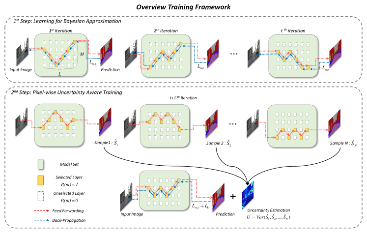
Figure 1: Overview of the proposed training framework. It consists of learning for Bayesian approximation and pixel-wise uncertainty aware training.

3 Proposed Method

In this section, we describe our proposed stochastic layer selection method and learning strategy. Figure 1 shows an overview of the proposed training framework. As shown in the Figure 1, a model set consist of $M$ submodels with $L$ layers. The model set is trained with two steps in our method. In the first step, the model set is constructed by randomly selected layers for each iteration. The model set is optimized by a segmentation loss function to be able to reliably predict the output from arbitrary models, which consist of random combinations of layers. In this step the model set is learned to predict segmentation map and estimate uncertainty. Then, in the second step, the model set is optimized by two loss functions. One is the segmentation loss function that is used in the first step and the other one is a pixel-wise uncertainty loss that encourages the network to learn from the uncertain part of the predicted segmentation map. These loss values are back-propagated to selected layers and update the corresponding weight parameters. For the testing, we sample $N$ segmentation maps with randomly selected layers. We use the mean of samples as a segmentation prediction and use the pixel variance as a predictive uncertainty.

3.1 Stochastic Layer Selection

In this section, we describe how to design the model set and how to select layers stochastically. The proposed model set consists of $M$ (where $M\geq 2$) parallel submodels and each submodel has $L$ layers. Then, we can sample a model with random variable ${P}_{l}(m)$ as follow

$${{P}_{l}}(m)=\left\{\begin{matrix}1,\ \text{if}\ Layer_{m}^{l}\ \text{is}\ \text{selected,}\\ 0,\ \text{otherwise}.\,\,\,\,\,\,\,\,\,\,\,\,\,\,\,\,\,\,\,\,\,\,\,\,\,\,\,\ \\ \end{matrix}\right.$$ (1)

In order to ensure that each layer is selected from one submodel, we constrain the ${{P}_{l}}(m)$ as follow

$$\sum\limits_{m=1}^{M}{{{P}_{l}}(m)=1},$$ (2)

$${P}_{l}\sim categorical({{x}_{1}},{{x}_{2}},...,{{x}_{M}};{{\mu}_{1}},{{\mu}_{2}},...,{{\mu}_{M}}),$$ (3)

where ${{P}_{l}}$ is a $1\times M$ dimension vector of categorical random variables with probability ${{\mu}_{m}}$ of being 1. Then, the total weight ($W$) and random selecting vector of the model set can be defined as follow

$$W=\begin{Bmatrix}{w}_{1,1}&\dots&{w}_{1,L}\\ \vdots&\ddots&\vdots\\ {w}_{M,1}&\dots&{w}_{M,L}\end{Bmatrix},$$ (4)

$$P=\begin{Bmatrix}{P}_{1}\\ \vdots\\ {P}_{L}\end{Bmatrix},$$ (5)

where ${w}_{m,l}$ denotes the weight of $Layer_{m}^{l}$. Then, we sample a model which has same structure of sub model with $P_{l}(m)$. The weights of sampled model can be represented as follow

$${w}^{Sample}=diag(P\times W).$$ (6)

In contrast to dropout method that apply masking the perceptrons, our proposed method applies categorical random variables to each layer. We can construct ${{M}^{L}}$ ensemble models only with $M$ submodels which have same structure while have different weights. Furthermore, since the distribution of categorical random variables follows Bernoulli distribution, the model set can estimate the posterior distribution over the model weight parameters by Bayesian approximation. Therefore, our model can leverage both the effect of ensemble model that improve predictive performance [9, 28], and Bayesian approximation.

3.2 Uncertainty Measure using Stochastic Layer Selection

By the stochastic layer selection method, we can construct a large number of ensemble models within the limited number of parameters. It is well known fact that ensemble model can predict uncertainty by approximating the posterior with an ensemble of sample distributions [10, 34, 28]. We leverage the ensemble learning to perform our probabilistic inference. For given trained model set, we sample $N$ models with the random layer selection as in Eq.1 and predict $N$ segmentation prediction $\mathbf{S}=\{{{\hat{S}}_{1}},{{\hat{S}}_{2}},...,{{\hat{S}}_{N}}\}$. To estimate uncertainty, we take a variance of predicted samples as $U=var\{{{\hat{S}}_{1}},{{\hat{S}}_{2}},...,{{\hat{S}}_{N}}\}$.

3.3 Learning with Stochastic Layer Selection

As shown in Figure 1, our proposed stochastic layer selection learning method consists of two steps. In the first step, we train model set to be able to predict reliable segmentation map and estimate uncertainty by Bayesian approximation. In the second step, we utilize predictive uncertainty to encourage the model to focus on uncertain predictions and gradually overcome its limitation.

3.3.1 Learning for Bayesian Approximation

In the first step, we train the model set to be able to predict uncertainty. To this end, we find the posterior distribution over the model weight parameters $W$, with the given training data $X$, and training label $Y$. The posterior distribution can be defined as $p(w|X,Y)$. We can estimate the posterior by variational approximation. This approximation can be formulated as follow

$${\mathcal{L}_{\operatorname{var}}}=-\sum\limits_{i=1}^{K}{\int\limits_{w}{{{q}_{\theta}}(w)\log p({{y}_{i}}|{{x}_{i}},w)dw}}+KL({{q}_{\theta}}(w)||p(w)),$$ (7)

where ${{q}_{\theta}}(w)$ denotes approximate posterior and $KL({{q}_{\theta}}(w)||p(w))$ denotes Kullback-Leibler (KL) divergence with true posterior. $K$ denotes the number of example in dataset. However, this form of distribution is intractable, since we have to integrate over the all data. Therefore, we approximate the posterior distribution by Monte Carlo method. This approximation can be written as

$${\mathcal{L}_{\operatorname{var}}}=-\frac{1}{BN}\sum\limits_{i=1}^{B}{{}}\sum\limits_{j=1}^{N}{\log p({{y}_{i}}|{{x}_{i}},{{{\hat{w}}}_{i,j}})}+KL({{q}_{\theta}}(w)||p(w)),$$ (8)

where $B$ and $N$ denote the size of a batch and the number of samples, respectively. ${{\hat{w}}_{i,j}}\sim{{q}_{\theta}}(w)$ denotes a sample from the approximate distribution. Note that randomized weights that have Bernoulli distribution can approximate model of the Gaussian process [13]. Then, it can be approximated by minimizing the KL divergence.

Since we select the layers along with categorical random distribution ($P_{l}$) that follows Bernoulli distribution, we can approximate posterior by replacing $\hat{w}_{i,j}\leftarrow{w}^{Sample}$ in Eq. 8. Therefore, we approximate our posterior by minimizing KL divergence. Since minimizing the KL divergence term has the same effect of minimizing the cross entropy loss [13] , we optimize the model by reducing the cross entropy loss with our stochastic layer selection inference. Therefore, in the first step, we train the model with cross entropy loss. It enables the model set reliably predict the segmentation map and estimate uncertainty. This step continues until the validation loss is converged.

3.3.2 Pixel-wise Uncertainty Aware Training

After the first training step is finished, in the second step, we improve the segmentation prediction by pixel-wise uncertainty loss, as illustrated in Figure 1. To this end, during the training, we generate pixel-wise uncertainty map $U_{i}=var\{{{\hat{S}}_{1}},{{\hat{S}}_{2}},...,{{\hat{S}}_{N}}\}$, where ${\hat{S}}_{n}$ denotes the sample prediction with randomly seleced layers. $U_{i}$ means the pixel-wise variations between $N$ samples. With the pixel-wise uncertainty map, the pixel-wise uncertainty loss function can be defined as follows

$${\mathcal{L}_{U}}=-\sum\limits_{i=1}{({{U}_{i}}\otimes{{Y}_{i}})\log({{U}_{i}}\otimes{{{\hat{Y}}}_{i}})},$$ (9)

$${{\hat{Y}}_{i}}=f({{X}_{i}},{{P}_{1}},{{P}_{2}},...,{{P}_{L}}),$$ (10)

where $i$ denotes the index of training image, and $f(\cdot)$ is a function that maps the given input image $X$ to segmentation map with selected layers. $\otimes$ denotes an element-wise multiplication. The re-weighting of uncertain areas with large weights allows the model to improve on these samples. Therefore, the pixel-wise uncertainty loss encourages the model gradually to improve its limitation. Finally, in the second training step, a total loss can be written as follows,

$${\mathcal{L}_{total}}=\underbrace{-\sum\limits_{i=1}{{{Y}_{i}}\log({{{\hat{Y}}}_{i}})}}_{\text{Cross Entropy}}-\underbrace{\lambda\sum\limits_{i=1}{({{U}_{i}}\otimes{{Y}_{i}})\log({{U}_{i}}\otimes{{{\hat{Y}}}_{i}})}}_{\text{Pixel-wise Uncertainty}},$$ (11)

where $\lambda$ denotes a balancing hyper-parameter. The algorithms for the training and the test are described in Appendix A.

4 Experiment

To verify the effectiveness of the proposed method, we evaluate our method on two possible safe-critical applications. Firstly, for the autonomous driving application, we use CamVid[6] dataset which is widely used for road scene understanding and uncertainty estimation. For the medical diagnosis, we use Transvaginal Ultrasound (TVUS) dataset which is an in-house dataset for the experiment.

4.1 Experiment Setting

4.1.1 CamVid Dataset

The dataset is a publically available semantic segmentation dataset for road scene understanding, which has applications for autonomous driving. The dataset is also widely used to analyze the predictive uncertainty [22, 20, 28, 37]. It consists of 367 training and 233 testing images of day and dusk scenes. Following the experimental protocol in [3], we use 11 classes such as road, building, cars, etc. To avoid overfitting, we conduct data augmentation (vertical flip, random crop, resize, and random rotation).

For the model set design, we use the FC-DenseNet 103 [21] as a submodel. Then, we construct a model set with two submodels (M=2). We define the layers as ’Dense Block’ unit for our model set. Therefore, in our experiments we set M=2 and L=11. This model set is annotated as DenseNet-2 in the following experiment table and figure. We optimize the model set by using RMS-Prop [44] with a learning rate of 0.001 and exponential decay of 0.995 after each epoch. To get the mean prediction and predictive uncertainty, we sample 50 times N=50.

4.1.2 TVUS Dataset

The private dataset is collected from three hospitals. The purpose of this dataset is to segment endometrium regions on Transvaginal Ultrasound (TVUS) image. The dataset can be used to diagnose infertility by considering the shape and size of the endometrium. All the images are annotated by experienced gynecologists. To minimize the annotation inconsistency between gynecologists, we define the 4 gynecological points (cavity tip, internal os, and two thickest points between the two basal layers) [31, 16, 36] with the gynecologists. Then, they tried to annotate the GT mask while considering the point definition. After that, they cross-checked the annotations of each other and eliminated inconsistent annotations. As a result, we could build a well-annotated database with 3,372 images and corresponding endometrium segmentation maps. The full size of the image is 256$\times$320. To avoid overfitting, we also conduct data augmentation (vertical & horizontal flip, random rotation). For the evaluation, we conduct 5 folds cross-validation.

For the model set design, we use an U-Net architecture [38] which is widely used for medical segmentation. Then, we construct a model set with two submodels ($M=2$). We duplicate the every convolution layer in U-Net. We train the model from scratch without any preprocessing. Therefore, in our experiments we set $M=2$ and $L=18$. This model set is annotated as U-Net-2. We optimize our model set using ADAM optimizer [25] with a fixed learning rate 0.0001. To get the mean prediction and predictive uncertainty, we sample 50 times ($N=50$).

4.2 Quantitative Evaluation

Table 1: Comparison of Mean Intersection over Union (mIoU) and the number of network parameter on CamVid dataset.

Method	mIoU	Number of
		Parameter (M)
SegNet [3]	46.4	29.5
FCN-8s [30]	57.0	134.5
DeepLab-LFOV [7]	61.6	37.3
DFANet [29]	64.7	-
Dilation8 [49]	65.3	-
Dilation8 + FSO [27]	66.1	140.8
DenseNet [21](Our Implementation)	66.9(66.4)	9.4
G-FRNet [1]	68.0	29.5
Bi-Senet [48]	68.7	49.0
Uncertainty-Based Method
Bayesian SegNet [22]	63.1	29.5
Bayesian SegNet-2 (ours)	64.5	59.0
Bayesian SegNet-2 + Pixel-wise	65.3	59.0
Uncertainty Loss (ours)
Kendall et al. [23]	67.5	9.4
DenseNet-2 (ours)	67.4	18.8
DenseNet-2 + Pixel-wise	68.2	18.8
Uncertainty Loss (ours)

Table 2: Dice and Jaccard coefficient comparison of our method and other methods on TVUS dataset. The fourth column denotes the number of each network parameter.

Method	Dice Coefficient	Jaccard Coefficient	Number of
			Parameter (M)
U-Net [38]	82.30	70.38	31.0
FCN-8s [30]	81.19	69.12	134.5
Dilation8 [49]	82.40	70.36	140.8
Endometrium SegNet [36]	82.67	70.46	-
Uncertainty-Based Method
U-Net + MC-dropout [33]	82.00	68.92	31.0
U-Net-2 (ours)	82.72	70.09	62.0
U-Net-2 + Pixel-wise	83.51	71.40	62.0
Uncertainty Loss (ours)

To demonstrate the advantage of proposed method, we compare with other methods on two different datasets. Table 1 shows the mean intersection over union (mIoU) score on Camvid dataset. The DenseNet-2 is trained by our stochastic layer selection method without pixel-wise uncertainty loss. The DenseNet-2 + Pixel-wise Uncertainty Loss is trained by our stochastic layer selection method with pixel-wise uncertainty loss. In the case of DenseNet-2 + Pixel-wise Uncertainty Loss, the mIoU score achieves 68.2%. It has been improved to 1.3% compared to original DenseNet. Also, compared with other semantic segmentation networks, our method shows comparable performance. Furthermore, we compare the proposed method with recent uncertainty-based semantic segmentation methods. Our method shows better performance than other uncertainty-based methods. We observe that, compare to DenseNet-2, DenseNet-2+Pixelwise Uncertainty Loss shows better performance. This result can be interpreted in a way that our pixel-wise uncertainty loss improves the network effectively by gradually reducing the uncertain region during training. Also, to verify applicability of the proposed method, we applied the proposed method to Bayesian SegNet [22]. The results show that our method also achieves better performance than Bayesian SegNet, which indicates that our method could be applicable to other segmentation model.

For further evaluation of our method in medical application, we conduct more experiments on a challenging TVUS dataset. Table 2 shows the comparison with the conventional segmentation networks (FCN-8s and Dilation8) and an Endometrium SegNet according to Dice Coefficient Score (DCS) and Jaccard Coefficient Score (JCS). In the case of U-Net-2 + Pixel-wise Uncertainty Loss, we achieve 83.51% in DCS and 71.40% in JCS respectively. It has improved to 1.21% compared to the original U-Net. To prove that the performance improvement is statistical significance, we conduct a paired t-test. The paired t-test provides the statistical evaluation and qualification procedure of the segmentation network. The performance improvement is statistically significant ($p$<0.01 by paired t-test). Our method is also higher than U-Net+MC-dropout which samples 50 times with dropout. The proposed U-Net + Pixel-wise Uncertainty Loss shows 1.51% higher performance than U-Net+MC-dropout [33]. Furthermore, it shows superior performance compared to Endometrium SegNet [36]. Since our method encourages the model to gradually learn the uncertain part by pixel-wise uncertainty loss, it shows better performance than other methods.

4.3 Quantitative Comparison with Ensemble Model

Table 3: Comparison with ensemble model and our proposed method.

# of Network	CamVid (DenseNet)		TVUS (U-Net)
	mIOU	# of Parameters (M)	Dice Coefficient	# of Parameters (M)
Ensemble (1)	66.4	9.4	82.30	31.0
Ensemble (2)	66.8	18.8	82.51	62.0
Ensemble (3)	67.0	28.2	83.12	93.1
Ensemble (4)	67.1	37.6	83.20	124.1
Ensemble (5)	67.2	47.0	83.38	155.1
Ours	68.2	18.8	83.51	62.0

One of the our main contributions is that our model efficiently generates ensemble models. Therefore, in this section, we verify the effectiveness of our method by comparing with the vanilla ensemble models in terms of the number of parameters and the performance. To this end, we trained five different networks (DenseNet, U-Net) separately and estimate mean prediction and uncertainty with 5 samples. For each training setting, we use the same training hyper-parameters, e.g., learning rate, training iteration, optimizer, etc. The initial weights are set differently for each network. Table 3 shows the experiment results according to the number of sub-network in the ensemble model. As shown in Table 3, in the case of CamVid dataset with DensNet, our method shows 1.4% higher mIoU than Ensemble (2) which has the same number of parameters. Also our method shows 0.13% higher mIoU than Ensemble (5) which has a large number of parameters than our method. In the case of TVUS dataset with U-Net, our method shows 1% higher mIoU than Ensemble (2) which has the same number of parameter. Also our method shows 0.2% higher mIoU than Ensemble (5) which has a large number of parameters than our method. These results show that the proposed method effectively generates the ensemble models.

4.4 Quantitative Evaluation with Uncertainty-based Pixel Rejection

In this section, we demonstrate that our method effectively predicts the uncertain regions. To verify this, we conduct uncertainty-based pixel rejection experiment. For the pixel rejection experiment, we normalize the estimated uncertainty map from 0 to 1. Then, by sorting the uncertainty in descending order, we remove the pixels that the models indicate high uncertainty. We evaluate the performance on the remaining pixels in testing images.

In the CamVid dataset, we reject the uncertain pixels from 0% to 20% of total testing image pixels with an interval of 2.5%. Then, we measure the mIoU with remaining pixels. Figure 2 (a) shows the pixel rejection results on CamVid dataset. For the DenseNet + MC-dropout and DenseNet + Pixel-wise Uncertainty Loss, we estimate uncertainty with 50 samples. The DenseNet Ensemble (5) is a simple ensemble model with five different DenseNet network. We train the networks separately with random weight initialization. Then, we estimate the uncertainty with variance of each network prediction. In the case of random rejection, we randomly remove the pixel. As shown in Figure 2 (a), removing the pixel randomly does not help to improve the performance. In the case of DenseNet Ensemble (5), by removing the uncertain pixel, the mIoU is increased. It shows better performance than MC-dropout method at the beginning. However, since the number of samples is limited, DensNet Ensemble (5) could not estimate uncertainty well than MC-dropout method. Note that the number of parameter increases to increase the number of sample in the vanilla ensemble model. The MC-dropout method shows better performance than ensemble model from the moment 10% of uncertain pixels are removed. In the case of our method, as the uncertain pixels are removed, the mIoU score increased. Also, it shows better performance than MC-dropout method.

In the TVUS dataset, we reject the uncertain pixels from 0% to 5% of total testing image pixels with an interval of 0.5%. Figure 2 (b) shows the pixel rejection results on TVUS dataset. For the U-Net + MC-dropout and U-Net + Pixel-wise Uncertainty Loss, we estimate with 50 samples. In the case of U-Net Ensemble (5), we trained five different U-net separately and estimate uncertainty with 5 samples. As shown in Figure 2 (b), the random rejection does not help to improve the performance. Also, in the case of the ensemble networks, the result shows same tendency as shown in the previous experiment. It could not indicate uncertain pixels well than MC-dropout method since its limitation of the number of samples. In the case of our method, as the uncertain pixels are removed, the dice coefficient score is increased. Also, it shows better performance than MC-dropout method. Note that although our method utilizes the uncertainty to improve the model performance in training, the uncertainty at the inference time is still meaningful to indicate the confidence of the model’s prediction. The proposed method can guarantee the performance by rejecting to operate on samples where it is likely to fail.

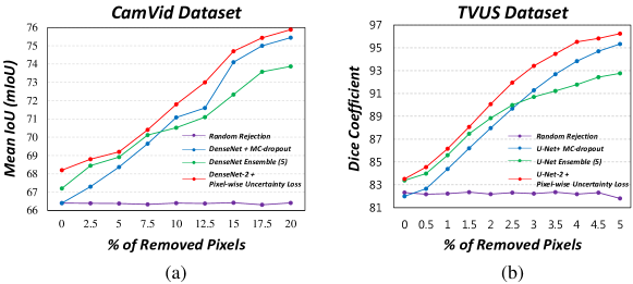
Figure 2: (a) Mean IOU according to pixel-wise rejection on CamVid dataset. (b) Dice coefficient according to pixel-wise rejection on TVUS dataset.

4.5 Qualitative Results

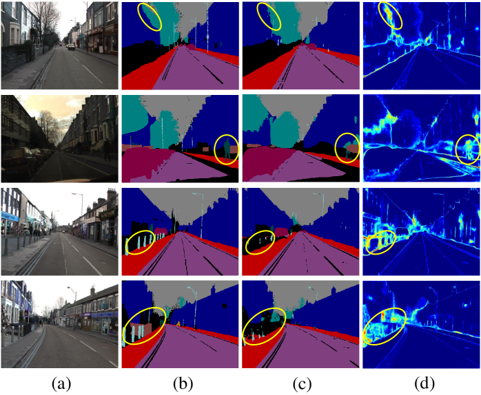
Figure 3: Qualitative results of segmentation and uncertainty estimation in our method on CamVid dataset. (a) is input images, (b) is ground truth maps, (c) is our mean prediction results with 50 samples, and (d) is our uncertainty map estimation results. The yellow circle denotes incorrect segmentation regions.

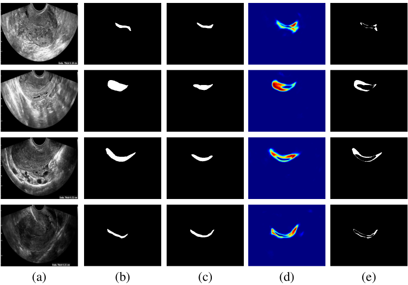
Figure 4: Qualitative results of segmentation and uncertainty estimation in our method on TVUS dataset. (a) is input images, (b) ground truth maps, (c) is mean prediction results with 50 samples, (d) uncertainty map by the proposed method, (e) is the difference between ground truth and segmentation results.

In this section, we visually observe the segmentation results and uncertainty estimation results. Figure 3 shows the predicted segmentation map and corresponding uncertainty map on CamVid dataset. As shown in the figure, although the network predicts incorrect segmentation results, the network estimate that the region is uncertain. In the case of the first and second rows, the network estimates uncertain regions where the object is hard to be observed because of the surrounding background and illumination. In the case of the third and fourth row, the network estimates uncertain regions where the unseen classes (black color in ground truth map) appeared. This allows the user to make comprehensive decisions by utilizing the uncertainty as well as predicted results.

For further evaluation, we visually observe the segmentation results and uncertainty estimation results on TVUS dataset. Figure 4 shows the predicted segmentation map and corresponding uncertainty map. As shown in the figure, the uncertain region and mis-segmentation region are similar. These results indicate that although the network predicts incorrectly, the user can make comprehensive decisions by utilizing the uncertainty.

4.6 Effect of number of sample

In this section, we analyze the effect of the number of sample in terms of mean prediction performance. Figure 5 (a) shows the mIoU score on CamVid dataset. Figure 5 (b) shows Dice Coefficient Score on TVUS dataset. Both results show that as the number of increase, the performance also increases. Then, our proposed method shows better performance with a few number of sample. In the Appendix C, we further discuss about pixel rejection results and quantitative results according the number of sample.

4.7 Discussion

Training time: Our method increases training time due to the multiple predictions for uncertainty estimation. However, the sampling process is only executed at the second training step. Therefore, the total training time does not increase so much compare to training two ensemble models. Also, our method takes less time than training five ensemble models while achieving better performance.

Generalization: In this paper, we verify the effectiveness of our method by setting $M=2$. With only 2 submodels, experimental results show that our method can get plausible uncertainty and achieve comparable performance. Note that we can theoretically generate 2048 ensemble models with DenseNet ($M=2$ and $L=11$) and 262,144 ensemble models with U-Net ($M=2$ and $L=18$). Additional results with $M=3$ are attached to the Appendix F.

Deep ensembles have been shown to be a promising approach to not only uncertainty estimation but also increase the adversarial robustness [28, 35]. Therefore, it is interesting to generalize our idea to other tasks such as classification and adversarial attack detection. In the Appendix E, we briefly verify that our method is robust to adversarial attacks.

Future work: The generalization of our idea to different tasks and various network architectures would be an interesting research agenda. In the autonomous driving system, not only segmentation but also depth estimation is important. It would be meaningful to extend our idea to other datasets and various network structures.

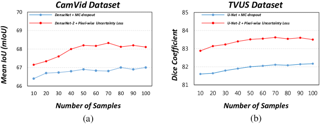
Figure 5: Effect of the number of sample on the performance. (a) Mean IOU measured on CamVid dataset. (b) Dice Coefficient measured on TVUS dataset.

5 Conclusion

This paper presents an efficient ensemble model generation method for uncertainty estimation through Bayesian approximation in segmentation. To generate ensemble models with a few numbers of sub-models, the stochastic layer selection learning method is proposed. The stochastic layer selection learning methods enabled the efficient generation of ensemble models. Then, through the stochastic layer selection learning, our ensemble model can estimate uncertainty with Bayesian approximation. Furthermore, the pixel-wise uncertainty loss is devised to use the uncertainty of the model in training. The re-weighting of uncertain areas with large weights allows the model to improve on these samples. Comprehensive and comparative experiments show that the proposed method could provide useful uncertainty information which can be used in the quality control and improve the predictive performance.

See pages - of ./Figure/Supplementary.pdf

References

- [1] Amirul Islam, M., Rochan, M., Bruce, N.D., Wang, Y.: Gated feedback refinement network for dense image labeling. In: Proceedings of the IEEE Conference on Computer Vision and Pattern Recognition. pp. 3751–3759 (2017)
- [2] Ashukha, A., Lyzhov, A., Molchanov, D., Vetrov, D.: Pitfalls of in-domain uncertainty estimation and ensembling in deep learning. arXiv preprint arXiv:2002.06470 (2020)
- [3] Badrinarayanan, V., Kendall, A., Cipolla, R.: Segnet: A deep convolutional encoder-decoder architecture for image segmentation. IEEE transactions on pattern analysis and machine intelligence 39(12), 2481–2495 (2017)
- [4] Bhattacharyya, A., Fritz, M., Schiele, B.: Long-term on-board prediction of people in traffic scenes under uncertainty. In: Proceedings of the IEEE Conference on Computer Vision and Pattern Recognition. pp. 4194–4202 (2018)
- [5] Blundell, C., Cornebise, J., Kavukcuoglu, K., Wierstra, D.: Weight uncertainty in neural networks. arXiv preprint arXiv:1505.05424 (2015)
- [6] Brostow, G.J., Fauqueur, J., Cipolla, R.: Semantic object classes in video: A high-definition ground truth database. Pattern Recognition Letters 30(2), 88–97 (2009)
- [7] Chen, L.C., Papandreou, G., Kokkinos, I., Murphy, K., Yuille, A.L.: Deeplab: Semantic image segmentation with deep convolutional nets, atrous convolution, and fully connected crfs. IEEE transactions on pattern analysis and machine intelligence 40(4), 834–848 (2017)
- [8] Chen, L.C., Zhu, Y., Papandreou, G., Schroff, F., Adam, H.: Encoder-decoder with atrous separable convolution for semantic image segmentation. In: Proceedings of the European conference on computer vision (ECCV). pp. 801–818 (2018)
- [9] Dietterich, T.G.: Ensemble methods in machine learning. In: International workshop on multiple classifier systems. pp. 1–15. Springer (2000)
- [10] Efron, B., Tibshirani, R.J.: An introduction to the bootstrap. CRC press (1994)
- [11] Feng, D., Rosenbaum, L., Dietmayer, K.: Towards safe autonomous driving: Capture uncertainty in the deep neural network for lidar 3d vehicle detection. In: 2018 21st International Conference on Intelligent Transportation Systems (ITSC). pp. 3266–3273. IEEE (2018)
- [12] Fort, S., Hu, H., Lakshminarayanan, B.: Deep ensembles: A loss landscape perspective. arXiv preprint arXiv:1912.02757 (2019)
- [13] Gal, Y., Ghahramani, Z.: Bayesian convolutional neural networks with bernoulli approximate variational inference. International Conference on Learning Representations Workshop (2016)
- [14] Gal, Y., Ghahramani, Z.: Dropout as a bayesian approximation: Representing model uncertainty in deep learning. In: international conference on machine learning. pp. 1050–1059 (2016)
- [15] Gal, Y., Islam, R., Ghahramani, Z.: Deep bayesian active learning with image data. In: Proceedings of the 34th International Conference on Machine Learning-Volume 70. pp. 1183–1192. JMLR. org (2017)
- [16] Gonen, Y., Casper, R.F., Jacobson, W., Blankier, J.: Endometrial thickness and growth during ovarian stimulation: a possible predictor of implantation in in vitro fertilization. Fertility and Sterility 52(3), 446–450 (1989)
- [17] Graves, A.: Practical variational inference for neural networks. In: Advances in neural information processing systems. pp. 2348–2356 (2011)
- [18] Gustafsson, F.K., Danelljan, M., Schön, T.B.: Evaluating scalable bayesian deep learning methods for robust computer vision. arXiv preprint arXiv:1906.01620 (2019)
- [19] Hernández-Lobato, J.M., Adams, R.: Probabilistic backpropagation for scalable learning of bayesian neural networks. In: International Conference on Machine Learning. pp. 1861–1869 (2015)
- [20] Huang, P.Y., Hsu, W.T., Chiu, C.Y., Wu, T.F., Sun, M.: Efficient uncertainty estimation for semantic segmentation in videos. In: Proceedings of the European Conference on Computer Vision (ECCV). pp. 520–535 (2018)
- [21] Jégou, S., Drozdzal, M., Vazquez, D., Romero, A., Bengio, Y.: The one hundred layers tiramisu: Fully convolutional densenets for semantic segmentation. In: Proceedings of the IEEE conference on computer vision and pattern recognition workshops. pp. 11–19 (2017)
- [22] Kendall, A., Badrinarayanan, V., Cipolla, R.: Bayesian segnet: Model uncertainty in deep convolutional encoder-decoder architectures for scene understanding. British Machine Vision Conference (BMVC) (2017)
- [23] Kendall, A., Gal, Y.: What uncertainties do we need in bayesian deep learning for computer vision? In: Advances in neural information processing systems. pp. 5574–5584 (2017)
- [24] Kendall, A., Gal, Y., Cipolla, R.: Multi-task learning using uncertainty to weigh losses for scene geometry and semantics. In: Proceedings of the IEEE conference on computer vision and pattern recognition. pp. 7482–7491 (2018)
- [25] Kingma, D.P., Ba, J.: Adam: A method for stochastic optimization. International Conference on Learning Representations (ICLR) (2014)
- [26] Kirsch, A., van Amersfoort, J., Gal, Y.: Batchbald: Efficient and diverse batch acquisition for deep bayesian active learning. In: Advances in Neural Information Processing Systems. pp. 7024–7035 (2019)
- [27] Kundu, A., Vineet, V., Koltun, V.: Feature space optimization for semantic video segmentation. In: Proceedings of the IEEE Conference on Computer Vision and Pattern Recognition. pp. 3168–3175 (2016)
- [28] Lakshminarayanan, B., Pritzel, A., Blundell, C.: Simple and scalable predictive uncertainty estimation using deep ensembles. In: Advances in neural information processing systems. pp. 6402–6413 (2017)
- [29] Li, H., Xiong, P., Fan, H., Sun, J.: Dfanet: Deep feature aggregation for real-time semantic segmentation. In: Proceedings of the IEEE Conference on Computer Vision and Pattern Recognition. pp. 9522–9531 (2019)
- [30] Long, J., Shelhamer, E., Darrell, T.: Fully convolutional networks for semantic segmentation. In: Proceedings of the IEEE conference on computer vision and pattern recognition. pp. 3431–3440 (2015)
- [31] Machtinger, R., Korach, J., Padoa, A., Fridman, E., Zolti, M., Segal, J., Yefet, Y., Goldenberg, M., Ben-Baruch, G.: Transvaginal ultrasound and diagnostic hysteroscopy as a predictor of endometrial polyps: risk factors for premalignancy and malignancy. International Journal of Gynecologic Cancer 15(2), 325–328 (2005)
- [32] Minka, T.P.: Bayesian model averaging is not model combination. Available electronically at http://www. stat. cmu. edu/minka/papers/bma. html pp. 1–2 (2000)
- [33] Nair, T., Precup, D., Arnold, D.L., Arbel, T.: Exploring uncertainty measures in deep networks for multiple sclerosis lesion detection and segmentation. Medical image analysis 59, 101557 (2020)
- [34] Osband, I., Blundell, C., Pritzel, A., Van Roy, B.: Deep exploration via bootstrapped dqn. In: Advances in neural information processing systems. pp. 4026–4034 (2016)
- [35] Pang, T., Xu, K., Du, C., Chen, N., Zhu, J.: Improving adversarial robustness via promoting ensemble diversity. arXiv preprint arXiv:1901.08846 (2019)
- [36] Park, H., Lee, H.J., Kim, H.G., Ro, Y.M., Shin, D., Lee, S.R., Kim, S.H., Kong, M.: Endometrium segmentation on tvus image using key-point discriminator. Medical physics (2019)
- [37] Postels, J., Ferroni, F., Coskun, H., Navab, N., Tombari, F.: Sampling-free epistemic uncertainty estimation using approximated variance propagation. In: Proceedings of the IEEE International Conference on Computer Vision. pp. 2931–2940 (2019)
- [38] Ronneberger, O., Fischer, P., Brox, T.: U-net: Convolutional networks for biomedical image segmentation. In: International Conference on Medical image computing and computer-assisted intervention. pp. 234–241. Springer (2015)
- [39] Roy, A.G., Conjeti, S., Navab, N., Wachinger, C., Initiative, A.D.N., et al.: Bayesian quicknat: model uncertainty in deep whole-brain segmentation for structure-wise quality control. NeuroImage 195, 11–22 (2019)
- [40] Rupprecht, C., Laina, I., DiPietro, R., Baust, M., Tombari, F., Navab, N., Hager, G.D.: Learning in an uncertain world: Representing ambiguity through multiple hypotheses. In: Proceedings of the IEEE International Conference on Computer Vision. pp. 3591–3600 (2017)
- [41] Seo, S., Seo, P.H., Han, B.: Learning for single-shot confidence calibration in deep neural networks through stochastic inferences. In: Proceedings of the IEEE Conference on Computer Vision and Pattern Recognition. pp. 9030–9038 (2019)
- [42] Snoek, J., Ovadia, Y., Fertig, E., Lakshminarayanan, B., Nowozin, S., Sculley, D., Dillon, J., Ren, J., Nado, Z.: Can you trust your model’s uncertainty? evaluating predictive uncertainty under dataset shift. In: Advances in Neural Information Processing Systems. pp. 13969–13980 (2019)
- [43] Srivastava, N., Hinton, G., Krizhevsky, A., Sutskever, I., Salakhutdinov, R.: Dropout: a simple way to prevent neural networks from overfitting. The journal of machine learning research 15(1), 1929–1958 (2014)
- [44] Tieleman, T., Hinton, G.: Lecture 6.5-rmsprop: Divide the gradient by a running average of its recent magnitude. COURSERA: Neural networks for machine learning 4(2), 26–31 (2012)
- [45] Tramèr, F., Kurakin, A., Papernot, N., Goodfellow, I., Boneh, D., McDaniel, P.: Ensemble adversarial training: Attacks and defenses. International Conference on Learning Representations (ICLR) (2018)
- [46] Valdenegro-Toro, M.: Deep sub-ensembles for fast uncertainty estimation in image classification. arXiv preprint arXiv:1910.08168 (2019)
- [47] Welling, M., Teh, Y.W.: Bayesian learning via stochastic gradient langevin dynamics. In: Proceedings of the 28th international conference on machine learning (ICML-11). pp. 681–688 (2011)
- [48] Yu, C., Wang, J., Peng, C., Gao, C., Yu, G., Sang, N.: Bisenet: Bilateral segmentation network for real-time semantic segmentation. In: Proceedings of the European Conference on Computer Vision (ECCV). pp. 325–341 (2018)
- [49] Yu, F., Koltun, V.: Multi-scale context aggregation by dilated convolutions. arXiv preprint arXiv:1511.07122 (2015)
- [50] Yuan, Y., Chen, X., Wang, J.: Object-contextual representations for semantic segmentation. arXiv preprint arXiv:1909.11065 (2019)
- [51] Zhao, H., Shi, J., Qi, X., Wang, X., Jia, J.: Pyramid scene parsing network. In: Proceedings of the IEEE conference on computer vision and pattern recognition. pp. 2881–2890 (2017)
- [52] Zhu, Y., Sapra, K., Reda, F.A., Shih, K.J., Newsam, S., Tao, A., Catanzaro, B.: Improving semantic segmentation via video propagation and label relaxation. In: Proceedings of the IEEE Conference on Computer Vision and Pattern Recognition. pp. 8856–8865 (2019)