Tensor Clustering with Planted Structures: Statistical Optimality and Computational Limits

Abstract

This paper studies the statistical and computational limits of high-order clustering with planted structures. We focus on two clustering models, constant high-order clustering (CHC) and rank-one higher-order clustering (ROHC), and study the methods and theory for testing whether a cluster exists (detection) and identifying the support of cluster (recovery).

Specifically, we identify the sharp boundaries of signal-to-noise ratio for which CHC and ROHC detection/recovery are statistically possible. We also develop the tight computational thresholds: when the signal-to-noise ratio is below these thresholds, we prove that polynomial-time algorithms cannot solve these problems under the computational hardness conjectures of hypergraphic planted clique (HPC) detection and hypergraphic planted dense subgraph (HPDS) recovery. We also propose polynomial-time tensor algorithms that achieve reliable detection and recovery when the signal-to-noise ratio is above these thresholds. Both sparsity and tensor structures yield the computational barriers in high-order tensor clustering. The interplay between them results in significant differences between high-order tensor clustering and matrix clustering in literature in aspects of statistical and computational phase transition diagrams, algorithmic approaches, hardness conjecture, and proof techniques. To our best knowledge, we are the first to give a thorough characterization of the statistical and computational trade-off for such a double computational-barrier problem. Finally, we provide evidence for the computational hardness conjectures of HPC detection (via low-degree polynomial and Metropolis methods) and HPDS recovery (via low-degree polynomial method).

and

1 Introduction

The high-dimensional tensor data have been increasingly prevalent in many domains, such as genetics, social sciences, engineering. In a wide range of applications, unsupervised analysis, in particular the high-order clustering, can be applied to discover the hidden modules in these high-dimensional tensor data. For example, in microbiome studies, microbiome samples are often measured across multiple body sites from multiple subjects (Faust et al., 2012; Flores et al., 2014), resulting in the three-way tensors with subjects, body sites, and bacteria taxa as three modes. It has been reported that multiple microbial taxa can coexist within or across multiple body sites and subjects can form different subpopulations (Faust et al., 2012). Similar data structures can also be found in multi-tissue multi-individual gene expression data (Wang, Fischer and Song, 2019). Mathematically, these patterns correspond to high-order clusters, i.e., the underlying multi-way block structures in the data tensor. We also refer readers to the recent survey (Henriques and Madeira, 2019) on high-order clustering in applications.

In the literature, a number of methods have been proposed for triclustering or high-order clustering of tensor data, such as divide and conquer (Li and Tuck, 2009), seed growth (Sim, Aung and Gopalkrishnan, 2010), stochastic approach (Amar et al., 2015), exhaustive approaches (Jiang et al., 2004), pattern-based approach (Ji, Tan and Tung, 2006), etc. However, the theoretical guarantees for those existing procedures are not well established to our best knowledge.

This paper aims to fill the void of theory in high-order clustering. Suppose we observe an $n_{1}\times\cdots\times n_{d}$-dimensional order-$d$ tensor ${\mathbfcal{Y}}$ that satisfies

$${\mathbfcal{Y}}={\mathbfcal{X}}+{\mathbfcal{Z}},$$ (1)

where ${\mathbfcal{X}}\in\mathbb{R}^{n_{1}\times\cdots\times n_{d}}$ is the underlying signal with planted structure and ${\mathbfcal{Z}}$ is the noise that has i.i.d standard normal distributed entries. Our goal is to detect or recover the “planted structure" of the signal ${\mathbfcal{X}}$. The specific problems in this paper are listed below.

1.1 Problem Formulations

First, we consider the signal tensor ${\mathbfcal{X}}$ that contains a constant planted structure:

$${\mathbfcal{X}}\in\mathscr{X}_{{\rm{CHC}}}(\mathbf{k},\mathbf{n},\lambda),\quad\mathscr{X}_{{\rm{CHC}}}(\mathbf{k},\mathbf{n},\lambda)=\left\{\lambda^{\prime}\mathbf{1}_{I_{1}}\circ\cdots\circ\mathbf{1}_{I_{d}}:I_{i}\subseteq[n_{i}],|I_{i}|=k_{i},\lambda^{\prime}\geq\lambda\right\}.$$ (2)

Here, “$\circ$" denotes the vector outer product, $\mathbf{1}_{I_{i}}$ is the $n_{i}$-dimensional indicator vector such that $(\mathbf{1}_{I_{i}})_{j}=1$ if $j\in I_{i}$ and $(\mathbf{1}_{I_{i}})_{j}=0$ if $j\notin I_{i}$; $\lambda$ represents the signal strength. We collectively denote $\mathbf{k}=(k_{1},\ldots,k_{d})$ and $\mathbf{n}=(n_{1},\ldots,n_{d})$ for convenience. The support of the planted structure of ${\mathbfcal{X}}$ is denoted as $\mathcal{S}({\mathbfcal{X}}):=(I_{1},\ldots,I_{d})$. We refer to this model (1)(2) as the constant high-order clustering (CHC). The constant planted clustering model in tensor or matrix biclustering (BC) data has been considered in a number of recent literature (see, e.g., Butucea and Ingster (2013); Butucea, Ingster and Suslina (2015); Sun and Nobel (2013); Brennan, Bresler and Huleihel (2018); Chi, Allen and Baraniuk (2017); Cai, Liang and Rakhlin (2017); Brennan, Bresler and Huleihel (2019); Kolar et al. (2011); Chen and Xu (2016); Xia and Zhou (2019)).

We also consider a more general setting that ${\mathbfcal{X}}$ contains a rank-one planted structure:

$${\mathbfcal{X}}\in\mathscr{X}_{{\rm{ROHC}}}(\mathbf{k},\mathbf{n},\mu),\quad\mathscr{X}_{{\rm{ROHC}}}(\mathbf{k},\mathbf{n},\mu)=\left\{\mu^{\prime}\mathbf{v}_{1}\circ\cdots\circ\mathbf{v}_{d}:\mathbf{v}_{i}\in\mathcal{V}_{n_{i},k_{i}},\mu^{\prime}\geq\mu\right\},$$ (3)

where

$$\mathcal{V}_{n,k}:=\left\{\mathbf{v}\in\mathbb{S}^{n-1}:k/C_{1}\leq\|\mathbf{v}\|_{0}\leq k\text{ and }k^{-1/2}\leq|\mathbf{v}_{i}|\leq C_{2}k^{-1/2}\text{ for }i\in S(\mathbf{v})\right\},\quad C_{1},C_{2}>1$$

is the set of all $k$-sparse unit vectors with near-uniform magnitude. Here $S(\mathbf{v})$ denotes the support of the vector $\mathbf{v}$ and its formal definition is given in Section 2. Throughout the paper, we refer to the model in (1)(3) as the rank-one high-order clustering (ROHC). Especially if $d=2$, i.e., in the matrix case, this model (rank-one submatrix (ROS)) was considered in Sun and Nobel (2013); Busygin, Prokopyev and Pardalos (2008); Madeira and Oliveira (2004); Brennan, Bresler and Huleihel (2018). For both models, we hope to answer the following questions on detection ($\mathcal{P}_{D}$) and recovery ($\mathcal{P}_{R}$):

1. When we can detect if any high-order cluster exists and when such conclusion cannot be made. To be specific, consider the following hypothesis tests:

   $$\begin{split}{\rm{CHC}}_{D}(\mathbf{n},\mathbf{k},\lambda):&\quad H_{0}:{\mathbfcal{X}}=\mathbf{0}\quad\text{v.s.}\quad\quad H_{1}:{\mathbfcal{X}}\in\mathscr{X}_{{\rm{CHC}}}(\mathbf{k},\mathbf{n},\lambda),\\ {\rm{ROHC}}_{D}(\mathbf{n},\mathbf{k},\mu):&\quad H_{0}:{\mathbfcal{X}}=\mathbf{0}\quad\text{v.s.}\quad\quad H_{1}:{\mathbfcal{X}}\in\mathscr{X}_{{\rm{ROHC}}}(\mathbf{k},\mathbf{n},\mu),\end{split}$$ (4)

   we ask when there is a sequence of algorithms that can achieve reliable detection, i.e., both type-I and II errors tend to zero.

2. How to recover the support of the cluster when it exists. Specifically, we assume $H_{1}$ holds and aim to develop an algorithm that recovers the support $S({\mathbfcal{X}})$ based on the observation of ${\mathbfcal{Y}}$. Denote the CHC and ROHC recovery problems considered in this paper as ${\rm{CHC}}_{R}(\mathbf{n},\mathbf{k},\lambda)$ and ${\rm{ROHC}}_{R}(\mathbf{n},\mathbf{k},\mu)$, respectively. We would like to know when there exists a sequence of algorithms that can achieve reliable recovery, i.e., the probability of correctly recovering $S({\mathbfcal{X}})$ tends to one.

We study the performance of both unconstrained-time algorithms and polynomial-time algorithms for both detection $\mathcal{P}_{D}$ and recovery $\mathcal{P}_{R}$. The class of unconstrained algorithms includes all procedures with unlimited computational resources, while an algorithm that runs in polynomial-time has access to poly($n$) independent random bits and must finish in poly$(n)$ time, where $n$ is the size of input. For convenience of exposition, we assume the explicit expressions can be exactly computed and $N(0,1)$ random variable can be sampled in $O(1)$ time.

1.2 Main Results

In this paper, we give a comprehensive characterization of the statistical and computational limits of the detection and recovery for both ${\rm{CHC}}$ and ${\rm{ROHC}}$ models. Denote $n:=\max_{i}n_{i},k:=\max_{i}k_{i}$, and assume $d$ is fixed. For technical convenience, our discussions are based on two asymptotic regimes:

$$\forall i\in[d],\quad n_{i}\to\infty,\quad k_{i}\to\infty\quad\text{and}\quad k_{i}/n_{i}\to 0;$$ (A1)

$$\begin{split}\text{or}\qquad&\text{for fixed $0\leq\alpha\leq 1,\beta\in\mathbb{R}$ },n\to\infty,\quad n_{1}=\cdots=n_{d}=\tilde{\Theta}(n),\\ &k=k_{1}=\cdots=k_{d}=\tilde{\Theta}(n^{\alpha}),\quad\lambda=\tilde{\Theta}(n^{-\beta}),\quad\mu/\sqrt{k^{d}}=\tilde{\Theta}(n^{-\beta}).\end{split}$$ (A2)

In (A2), $\alpha$ and $\beta$ represent the sparsity level and the signal strength of the cluster, respectively. The cluster becomes sparser as $\alpha$ decreases and the signal becomes stronger as $\beta$ decreases. A rescaling of $\mu$ in (A2) is to make the magnitude of normalized entries in cluster of ${\rm{ROHC}}$ to be approximately one, which enables a valid comparison between the computational hardness of ${\rm{CHC}}$ and ${\rm{ROHC}}$.

The following informal statements summarize the main results of this paper.

Theorem 1 (Informal: Phase Transitions in CHC)

Define

$$\begin{split}&\beta^{s}_{{\rm{CHC}}_{D}}:=\left(d\alpha-d/2\right)\lor(d-1)\alpha/2,\quad\beta^{s}_{{\rm{CHC}}_{R}}:=(d-1)\alpha/2,\\ &\beta^{c}_{{\rm{CHC}}_{D}}:=\left(d\alpha-d/2\right)\lor 0,\quad\beta^{c}_{{\rm{CHC}}_{R}}:=\left((d-1)\alpha-(d-1)/2\right)\lor 0.\end{split}$$ (5)

Under the asymptotic regime (A2), the statistical and computational limits of ${\rm{CHC}}_{D}(\mathbf{k},\mathbf{n},\lambda)$ and ${\rm{CHC}}_{R}(\mathbf{k},\mathbf{n},\lambda)$ exhibit the following phase transitions:

• CHC Detection:

  1. $\beta>\beta^{s}_{{\rm{CHC}}_{D}}$: reliable detection is information-theoretically impossible.

  2. $\beta^{c}_{{\rm{CHC}}_{D}}<\beta<\beta^{s}_{{\rm{CHC}}_{D}}$: the computational inefficient test $\psi_{{\rm{CHC}}_{D}}^{s}$ in Section 4.1 succeeds, but polynomial-time reliable detection is impossible based on the hypergraphic planted clique (HPC) conjecture (Conjecture 1).

  3. $\beta<\beta^{c}_{{\rm{CHC}}_{D}}$: the polynomial-time test $\psi_{{\rm{CHC}}_{D}}^{c}$ in Section 4.2 based on combination of sum and max statistics succeeds.

• CHC Recovery:

  1. $\beta>\beta^{s}_{{\rm{CHC}}_{R}}$: reliable recovery is information-theoretically impossible.

  2. $\beta^{c}_{{\rm{CHC}}_{D}}<\beta<\beta^{s}_{{\rm{CHC}}_{R}}$: the exhaustive search (Algorithm 1) succeeds, but polynomial-time reliable recovery is impossible based on HPC conjecture (Conjecture 1) and hypergraphic planted dense subgraph (HPDS) recovery conjecture (Conjecture 2).

  3. $\beta<\beta^{c}_{{\rm{CHC}}_{D}}$: the combination of polynomial-time Algorithms 3 and 5 succeeds.

Theorem 2 (Informal: Phase Transitions in ROHC)

Define

$$\begin{split}&\beta^{s}_{{\rm{ROHC}}}=\beta^{s}_{{\rm{ROHC}}_{D}}=\beta^{s}_{{\rm{ROHC}}_{R}}:=(d-1)\alpha/2,\\ &\beta^{c}_{{\rm{ROHC}}}=\beta^{c}_{{\rm{ROHC}}_{D}}=\beta^{c}_{{\rm{ROHC}}_{R}}:=\left(\alpha d/2-d/4\right)\lor 0.\end{split}$$ (6)

Under the asymptotic regime (A2), the statistical and computational limits of ${\rm{ROHC}}_{D}(\mathbf{k},\mathbf{n},\mu)$ and ${\rm{ROHC}}_{R}(\mathbf{k},\mathbf{n},\mu)$ exhibit the following phase transitions:

1. $\beta>\beta^{s}_{{\rm{ROHC}}}$: reliable detection and recovery are information-theoretically impossible.

2. $\beta^{c}_{{\rm{ROHC}}}<\beta<\beta^{s}_{{\rm{ROHC}}}$: the computational inefficient test $\psi_{{\rm{ROHC}}_{D}}^{s}$ in Section 4.1 succeeds in detection and the search Algorithm 2 succeeds in recovery, but polynomial-time reliable detection and recovery are impossible based on the HPC conjecture (Conjecture 1).

3. $\beta<\beta^{c}_{{\rm{ROHC}}}$: the polynomial-time test $\psi_{{\rm{ROHC}}_{D}}^{c}$ in Section 4.2 succeeds in detection and the combination of polynomial-time Algorithms 3 and 4 succeeds in recovery.

In Table 1, we summarize the statistical and computational limits in Theorems 1 and 2 in terms of the original parameters $k,n,\lambda,\mu$ and provide the corresponding algorithms that achieve these limits.

	${\rm{CHC}}_{D}$	${\rm{CHC}}_{R}$	${\rm{ROHC}}_{D}$ & ${\rm{ROHC}}_{R}$
Impossible	$\lambda^{2}\ll\frac{n^{d}}{k^{2d}}\wedge\frac{1}{k^{d-1}}$	$\lambda^{2}\ll\frac{1}{k^{d-1}}$	$\frac{\mu^{2}}{k^{d}}\ll\frac{1}{k^{d-1}}$
Hard	$\frac{n^{d}}{k^{2d}}\wedge\frac{1}{k^{d-1}}\lesssim\lambda^{2}\ll\frac{n^{d}}{k^{2d}}\wedge 1$	$\frac{1}{k^{d-1}}\lesssim\lambda^{2}\ll\frac{n^{d-1}}{k^{2(d-1)}}\wedge 1$	$\frac{1}{k^{d-1}}\lesssim\frac{\mu^{2}}{k^{d}}\ll\frac{n^{d/2}}{k^{d}}\wedge 1$
Algorithms	$\psi_{{\rm{CHC}}_{D}}^{s}$	Alg 1	$\psi_{{\rm{ROHC}}_{D}}^{s}$& Alg 2
Easy	$\lambda^{2}\gtrsim\frac{n^{d}}{k^{2d}}\wedge 1$	$\lambda^{2}\gtrsim\frac{n^{d-1}}{k^{2(d-1)}}\wedge 1$	$\frac{\mu^{2}}{k^{d}}\gtrsim\frac{n^{d/2}}{k^{d}}\wedge 1$
Algorithms	$\psi_{{\rm{CHC}}_{D}}^{c}$	Algs 3 and 5	$\psi_{{\rm{ROHC}}_{D}}^{c}$ & Algs 3 and 4

Table 1: Phase transition and algorithms for detection and recovery in CHC and ROHC under the asymptotic regime (A2). Here, easy, hard, and impossible mean polynomial-time solvable, unconstrained-time solvable but polynomial-time unsolvable, and unconstrained-time unsolvable, respectively.

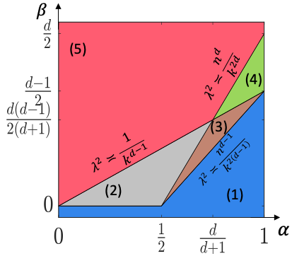
(a) Constant high-order clustering (${\rm{CHC}}$)

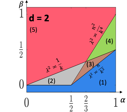
(b) Matrix biclustering (${\rm{BC}}$)

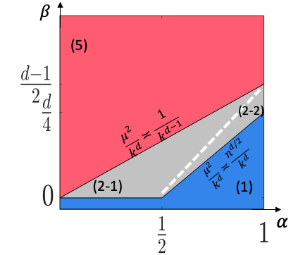
(c) Rank-one high-order clustering (${\rm{ROHC}}$)

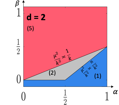
(d) Rank-one submatrix clustering (${\rm{ROS}}$)

Figure 1: Statistical and computational phase transition diagrams for constant high-order and rank-one high-order ($d\geq 3$) clustering models (CHC and ROHC) (left two panels) and constant biclustering and rank-one submatrix ($d=2$) clustering models (BC and ROS) (right two panels) under asymptotic regime (A2). Meaning of each region: (1) all problems detection and recovery both easy; (2),(2-1),(2-2) all problems detection hard and recovery hard; (3) CHC and BC detection easy and recovery hard; (4) CHC and BC detection easy and recovery impossible; (5) all problems detection and recovery impossible.

We also illustrate the phase transition diagrams for both ${\rm{CHC}},{\rm{ROHC}}$ $(d\geq 3)$ in Figure 1, Panels (a) and (c). When $d=2$, the phase transition diagrams in Panels (a) and (c) of Figure 1 reduce to constant biclustering (${\rm{BC}}$) diagram (Ma and Wu, 2015; Cai, Liang and Rakhlin, 2017; Brennan, Bresler and Huleihel, 2018; Chen and Xu, 2016) and rank-one submatrix (${\rm{ROS}}$) diagram (Brennan, Bresler and Huleihel, 2018) in Panels (b) and (d) of Figure 1.

1.3 Comparison with Matrix Clustering and Our Contributions

The high-order ($d\geq 3$) clustering problems show many distinct aspects from their matrix counterparts ($d=2$). We summarize the differences and highlight our contributions in the aspects of phase transition diagrams, algorithms, hardness conjecture, and proof techniques below.

(Phase transition diagrams) We can see the order-$d$ ($d\geq 3$) tensor clustering has an additional regime: (2-2) in Figure 1 Panel (c). Specifically if $d=2$, ${\rm{CHC}}_{R},{\rm{ROHC}}_{R}$ become ${\rm{BC}}_{R},{\rm{ROS}}_{R}$ that share the same computational limit and there is no gap between the statistical limit and computational efficiency for $\alpha=1$ in ${\rm{ROS}}_{R}$ (see Panels (b) and (d), Figure 1). If $d\geq 3$, we need a strictly stronger signal-to-noise ratio to solve ${\rm{ROHC}}_{R}$ than ${\rm{CHC}}_{R}$ and there is always a gap between the statistical optimality and computational efficiency for ${\rm{ROHC}}_{R}$. This difference roots in two level computation barriers, sparsity and tensor structure, in high-order ($d\geq 3$) clustering. To our best knowledge, we are the first to characterize such double computational barriers.

(Algorithms) In addition, we develop new algorithms for high-order clustering. For ${\rm{CHC}}_{R}$ and ${\rm{ROHC}}_{R}$, we introduce polynomial-time algorithms Power-iteration (Algorithm 4), Aggregated-SVD (Algorithm 5), both of which can be viewed as high-order analogues of the matrix spectral clustering. Also, see Section 1.4 for a comparison with the methods in the literature. We compare these algorithms and the exhaustive search (Algorithms 1 and 2) under the asymptotic regime (A2) in Figure 2. Compared to matrix clustering recovery diagram, i.e. Figure 1(d), a new Regime (2) appears in the high-order ($d\geq 3$) clustering diagram. Different from the matrix clustering, where the polynomial-time spectral method reaches the computational limits for both ${\rm{BC}}_{R}$ and ${\rm{ROS}}_{R}$ when $\frac{1}{2}\leq\alpha\leq 1$, the optimal polynomial-time algorithms for ${\rm{CHC}}_{R}$ and ${\rm{ROHC}}_{R}$ are distinct: Power-iteration is optimal for ${\rm{ROHC}}_{R}$ but is suboptimal for ${\rm{CHC}}_{R}$; the Aggregated-SVD is optimal for ${\rm{CHC}}_{R}$ but does not apply for ${\rm{ROHC}}_{R}$. This difference stems from the unique tensor algebraic structure in CHC.

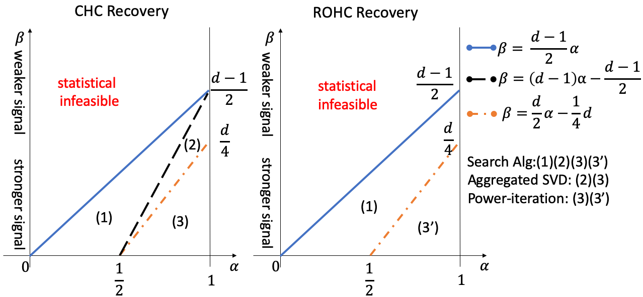
Figure 2: ${\rm{CHC}}_{R}$ and ${\rm{ROHC}}_{R}$ diagrams for Exhaustive search, Aggregated-SVD and Power-iteration algorithms under asymptotic regime (A2). In the right bottom corner, we provide the feasible signal-to-noise ratio regimes for each algorithm.

(Hardness conjecture) We adopt the average-case reduction approach to establish the computational lower bounds. It would be ideal to do average-case reduction from the commonly raised conjectures, such as the planted clique (PC) detection or Boolean satisfiability (SAT), so that all of the hardness results of these well-studied conjectures can be inherited to the target problem. However, this route is complicated by the multiway structure in the high-order clustering. Instead, we apply a new average-case reduction scheme from hypergraphic planted clique (HPC) and the hypergraphic planted dense subgraph (HPDS) since HPC and HPDS have a more natural tensor structure that enables a more straightforward average-case reduction. Despite the widely studied planted clique (PC) and planted dense subgraph (PDS) in literature, the HPC and HPDS are far less understood and so are their computational hardness conjectures. The relationship between the computational hardness of PC and HPC remains an open problem (Luo and Zhang, 2020a). This paper is among the first to explore the average computational complexities of HPC and HPDS. To provide evidence for the computation hardness conjecture, we show a class of powerful algorithms, including the polynomial-time low-degree polynomials and Metropolis algorithms, are not able to solve HPC detection unless the clique size is sufficiently large. Also, we show low-degree polynomial method only succeeds in HPDS recovery in a restricted parameter regime. These results on HPC and HPDS may be of independent interests in analyzing average-case computational complexity, given the steadily increasing popularity on tensor data analysis recently and the commonly observed statistical-computational gaps therein (Richard and Montanari, 2014; Barak and Moitra, 2016; Zhang and Xia, 2018; Perry et al., 2020; Hopkins, Shi and Steurer, 2015; Lesieur et al., 2017; Wein, El Alaoui and Moore, 2019; Dudeja and Hsu, 2021).

(Proof techniques) The theoretical analysis in high-order clustering incorporates sparsity, low-rankness, and tensor algebra simultaneously, which is significantly more challenging than its counterpart in matrix clustering. Specifically, to prove the statistical lower bound of ${\rm{ROHC}}_{D}$, we introduce the new Lemma 8, which gives an upper bound for the moment generating function of any power of a symmetric random walk on $\mathbb{Z}$ stopped after a hypergeometric distributed number of steps. This lemma is proved by utilizing Hoeffding’s inequality and the tail bound integration, which is different from the literature and can be of independent interest. To prove the statistical lower bound of ${\rm{CHC}}_{D}$, we introduce a new technique that “sequentially decompose event" to bound the second moment of the truncated likelihood ratio (see Lemma 5). To prove the computational lower bounds, we introduce new average-case reduction schemes from ${\rm{HPC}}$ and ${\rm{HPDS}}$, including a new reduction technique of tensor reflection cloning (Algorithm 7). This technique spreads the signal in the planted high-order cluster along each mode evenly, maintains the independence of entries in the tensor, and only mildly reduces the signal magnitude.

1.4 Related Literature

This work is related to a wide range of literature on biclustering, tensor decomposition, tensor SVD, and theory of computation. When the order of the observation $d=2$, the problem (1) reduces to the matrix clustering (Ames and Vavasis, 2011; Butucea, Ingster and Suslina, 2015; Chi, Allen and Baraniuk, 2017; Mankad and Michailidis, 2014; Tanay, Sharan and Shamir, 2002; Busygin, Prokopyev and Pardalos, 2008). The statistical and computational limits of matrix clustering have been extensively studied in the literature (Balakrishnan et al., 2011; Kolar et al., 2011; Butucea and Ingster, 2013; Ma and Wu, 2015; Chen and Xu, 2016; Cai, Liang and Rakhlin, 2017; Brennan, Bresler and Huleihel, 2018, 2019; Schramm and Wein, 2020). As discussed in Section 1.3, the high-order ($d\geq 3$) tensor clustering exhibits significant differences from the matrix problems in various aspects.

Another related topic is on tensor decomposition and best low-rank tensor approximation. Although the best low-rank matrix approximation can be efficiently solved by the matrix singular value decomposition (Eckart$-$Young$-$Mirsky Theorem), the best low-rank tensor approximation is NP-hard to calculate in general (Hillar and Lim, 2013). Various polynomial-time algorithms, which can be seen as the polynomial-time relaxations of the best low-rank tensor approximation, have been proposed in the literature, including the Newton method (Zhang and Golub, 2001), alternating minimization (Zhang and Golub, 2001; Richard and Montanari, 2014), high-order singular value decomposition (De Lathauwer, De Moor and Vandewalle, 2000a), high-order orthogonal iteration (De Lathauwer, De Moor and Vandewalle, 2000b), $k$-means power iteration (Anandkumar, Ge and Janzamin, 2014; Sun et al., 2017), sparse high-order singular value decomposition (Zhang and Han, 2019), regularized gradient descent (Han, Willett and Zhang, 2020), etc. The readers are referred to surveys Kolda and Bader (2009); Cichocki et al. (2015). Departing from most of these previous results, the high-order clustering considered this paper involves both sparsity and low-rankness structures, which requires new methods and theoretical analysis as discussed in Section 1.3.

Our work is also related to a line of literature on average-case computational hardness and the statistical and computational trade-offs. The average-case reduction approach has been commonly used to show computational lower bounds for many recent high-dimensional problems, such as testing $k$-wise independence (Alon et al., 2007), biclustering (Ma and Wu, 2015; Cai, Liang and Rakhlin, 2017; Cai et al., 2020), community detection (Hajek, Wu and Xu, 2015), RIP certification (Wang, Berthet and Plan, 2016; Koiran and Zouzias, 2014), matrix completion (Chen, 2015), sparse PCA (Berthet and Rigollet, 2013a, b; Brennan, Bresler and Huleihel, 2018; Gao, Ma and Zhou, 2017; Wang, Berthet and Samworth, 2016; Brennan and Bresler, 2019a), universal submatrix detection (Brennan, Bresler and Huleihel, 2019), sparse mixture and robust estimation (Brennan and Bresler, 2019b), a financial model with asymmetry information (Arora et al., 2011), finding dense common subgraphs (Charikar, Naamad and Wu, 2018), graph logistic regression (Berthet and Baldin, 2020), online local learning (Awasthi et al., 2015). See also a web of average-case reduction to a number of problems in Brennan, Bresler and Huleihel (2018); Brennan and Bresler (2020) and a recent survey (Wu and Xu, 2021). The average-case reduction is delicate, requiring that a distribution over instances in a conjecturally hard problem be mapped precisely to the target distribution. For this reason, many recent literature turn to show computational hardness results under the restricted models of computation, such as sum of squares (Ma and Wigderson, 2015; Hopkins et al., 2017; Barak et al., 2019), statistical query (Feldman et al., 2017; Diakonikolas, Kane and Stewart, 2017; Diakonikolas, Kong and Stewart, 2019; Feldman, Perkins and Vempala, 2018; Wang, Gu and Liu, 2015; Fan et al., 2018; Kannan and Vempala, 2017), class of circuit (Rossman, 2008, 2014), convex relaxation (Chandrasekaran and Jordan, 2013), local algorithms (Gamarnik and Sudan, 2014), meta-algorithms based on low-degree polynomials (Hopkins and Steurer, 2017; Kunisky, Wein and Bandeira, 2019) and others. As discussed in Section 1.3, this paper is among the first to investigate the hypergraphic planted clique (HPC) and hypergraphic planted dense subgraph (HPDS) problems and their computational hardness. We perform new average-case reduction scheme from these conjectures and develop the computational lower bounds for CHC and ROHC.

1.5 Organization

The rest of this article is organized as follows. After a brief introduction of notation and preliminaries in Section 2, the statistical limits of high-order cluster recovery and detection are given in Sections 3 and 4, respectively. In Section 5, we establish the computational limits of high-order clustering, along with the hypergraphic planted clique (HPC) and hypergraphic planted dense subgraph (HPDS) models, computational hardness conjectures, and evidence. Discussion and future work are given in Section 6. The technical proofs are collected in supplementary materials Luo and Zhang (2020b).

2 Notation and Definitions

The following notation will be used throughout this article. For any non-negative integer $n$, let $[n]=\{1,\ldots,n\}$. The lowercase letters (e.g., $a,b$), lowercase boldface letters (e.g., $\mathbf{u},\mathbf{v}$), uppercase boldface letters (e.g., ${\mathbf{A}},{\mathbf{U}}$), and boldface calligraphic letters (e.g., ${\mathbfcal{A}},{\mathbfcal{X}}$) are used to denote scalars, vectors, matrices, and order-3-or-higher tensors respectively. For any two series of numbers, say $\{a_{n}\}$ and $\{b_{n}\}$, denote $a\asymp b$ if there exist uniform constants $c,C>0$ such that $ca_{n}\leq b_{n}\leq Ca_{n},\forall n$; and $a=\Omega(b)$ if there exists uniform constant $c>0$ such that $a_{n}\geq cb_{n},\forall n$. The notation $a=\tilde{\Theta}(b)$ and $a\gg b$ mean $\lim_{n\to\infty}a_{n}/n=\lim_{n\to\infty}b_{n}/n$ and $\lim_{n\to\infty}\log(a_{n})/\log n>\lim_{n\to\infty}\log(b_{n})/\log n$, respectively. $a\lesssim b$ means $a\leq b$ up to polylogarithmic factors in $n$. We use bracket subscripts to denote sub-vectors, sub-matrices, and sub-tensors. For example, $\mathbf{v}_{[2:r]}$ is the vector with the $2$nd to $r$th entries of $\mathbf{v}$; ${\mathbf{D}}_{[(r+1):n_{1},:]}$ contains the $(r+1)$-th to the $n_{1}$-th rows of ${\mathbf{D}}$; ${\mathbfcal{A}}_{[1:s_{1},1:s_{2},1:s_{3}]}$ is the $s_{1}$-by-$s_{2}$-by-$s_{3}$ sub-tensor of ${\mathbfcal{A}}$ with index set $\{(i_{1},i_{2},i_{3}):1\leq i_{1}\leq s_{1},1\leq i_{2}\leq s_{2},1\leq i_{3}\leq s_{3}\}$. For any vector $\mathbf{v}\in\mathbb{R}^{n_{1}}$, define its $\ell_{2}$ norm as $\|\mathbf{v}\|_{2}=\left(\sum_{i}|\mathbf{v}_{i}|^{2}\right)^{1/2}$ and $\|\mathbf{v}\|_{0}$ is defined to be the number of non-zero entries in $\mathbf{v}$. Given vectors $\{\mathbf{v}_{i}\}_{i=1}^{d}\in\mathbb{R}^{n_{i}}$, the outer product ${\mathbfcal{A}}\in\mathbb{R}^{n_{1}\times\cdots\times n_{d}}=\mathbf{v}_{1}\circ\cdots\circ\mathbf{v}_{d}$ is defined such that ${\mathbfcal{A}}_{[i_{1},\ldots,i_{d}]}=(\mathbf{v}_{1})_{i_{1}}\cdots(\mathbf{v}_{d})_{i_{d}}$. For any event $A$, let $\mathbb{P}(A)$ be the probability that $A$ occurs.

For any order-$d$ tensor ${\mathbfcal{A}}\in\mathbb{R}^{n_{1}\times\cdots\times n_{d}}$. The matricization $\mathcal{M}(\cdot)$ is the operation that unfolds or flattens the order-$d$ tensor ${\mathbfcal{A}}\in\mathbb{R}^{n_{1}\times\cdots\times n_{d}}$ into the matrix $\mathcal{M}_{z}({\mathbfcal{A}})\in\mathbb{R}^{n_{z}\times\prod_{j\neq z}n_{j}}$ for $z=1,\ldots,d$. Specifically, the mode-$z$ matricization of ${\mathbfcal{A}}$ is formally defined as

$${\mathbfcal{A}}_{[i_{1},\ldots,i_{d}]}=\left(\mathcal{M}_{z}({\mathbfcal{A}})\right)_{\left[i_{z},j\right]},\quad j=1+\sum_{\begin{subarray}{c}l=1\\ l\neq z\end{subarray}}^{d}\left\{(i_{l}-1)\prod_{\begin{subarray}{c}m=1\\ m\neq z\end{subarray}}^{l-1}n_{m}\right\}$$

for any $1\leq i_{l}\leq n_{l},l=1,\ldots,d$. Also see (Kolda and Bader, 2009, Section 2.4) for more discussions on tensor matricizations. The mode-$z$ product of ${\mathbfcal{A}}\in\mathbb{R}^{n_{1}\times\cdots\times n_{d}}$ with a matrix ${\mathbf{U}}\in\mathbb{R}^{k_{z}\times n_{z}}$ is denoted by ${\mathbfcal{A}}\times_{z}{\mathbf{U}}$ and is of size $n_{1}\times\cdots\times n_{z-1}\times k_{z}\times n_{z+1}\times\cdots\times n_{d}$, such that

$$({\mathbfcal{A}}\times_{z}{\mathbf{U}})_{[i_{1},\ldots,i_{z-1},j,i_{z+1},\ldots,i_{d}]}=\sum_{i_{z}=1}^{n_{z}}{\mathbfcal{A}}_{[i_{1},i_{2},\ldots,i_{d}]}{\mathbf{U}}_{[j,i_{z}]}.$$

For any two distinct $k_{1},k_{2}\in[d]\,(k_{1}<k_{2})$ and $j_{1}\in[n_{k_{1}}]$ and $j_{2}\in[n_{k_{2}}]$, we denote

$${\mathbfcal{A}}^{(k_{1},k_{2})}_{j_{1},j_{2}}={\mathbfcal{A}}_{\Big{[}:,~{}\ldots~{},:,\underbrace{j_{1}}_{k_{1}\text{th index}},:,~{}\ldots,~{}:,\underbrace{j_{2}}_{k_{2}\text{th index}},:~{}\ldots,~{}:\Big{]}}\in\mathbb{R}^{n_{1}\times\cdots\times n_{k_{1}-1}\times n_{k_{1}+1}\times\cdots\times n_{k_{2}-1}\times n_{k_{2}+1}\times\cdots\times n_{d}}$$

as a subtensor of ${\mathbfcal{A}}$. The support of an order-$d$ tensor ${\mathbfcal{X}}\in\mathbb{R}^{n_{1}\times\cdots\times n_{d}}$ is denoted by $S({\mathbfcal{X}}):=(I_{1},\cdots,I_{d})$ where $I_{j}\in\mathbb{R}^{n_{j}}$ and $(I_{j})_{i}$ equals to zero when $\mathcal{M}_{j}({\mathbfcal{X}})_{[i,:]}$ is a zero vector and equals to one otherwise. In particular, when the tensor order is $1$, we simply have the support of a vector $\mathbf{v}$ is $S(\mathbf{v})=\{j:\mathbf{v}_{j}\neq 0\}$.

Given a distribution $Q$, let $Q^{\otimes n}$ be the distribution of $(X_{1},\ldots,X_{n})$ if $\{X_{i}\}_{i=1}^{n}$ are i.i.d. copies of $Q$. Similarly, let $Q^{\otimes m\times n}$ and $Q^{\otimes(n^{\otimes d})}$ denote the distribution on $\mathbb{R}^{m\times n}$ and $\mathbb{R}^{n^{\otimes d}}$ with i.i.d. entries distributed as $Q$. Here $n^{\otimes d}:=n\times n\times\cdots\times n$ denotes the order-$d$ Cartesian product. In addition, we use $C,C_{1},C_{2},c$ and other variations to represent the large and small constants, whose actual values may vary from line to line.

Next, we formally define the statistical and computational risks to quantify the fundamental limits of high-order clustering. First, we define the risk of testing procedure $\phi_{D}({\mathbfcal{Y}})\in\{0,1\}$ as the sum of Type-I and Type-II errors for detection problems ${\rm{CHC}}_{D}$ and ${\rm{ROHC}}_{D}$:

$$\mathcal{E}_{\mathcal{P}_{D}}(\phi_{D})=\mathbb{P}_{0}(\phi_{D}({\mathbfcal{Y}})=1)+\sup_{\begin{subarray}{c}{\mathbfcal{X}}\in\mathscr{X}_{{\rm{CHC}}}(\mathbf{k},\mathbf{n},\lambda)\\ (\text{or }{\mathbfcal{X}}\in\mathscr{X}_{{\rm{ROHC}}}(\mathbf{k},\mathbf{n},\mu))\end{subarray}}\mathbb{P}_{{\mathbfcal{X}}}(\phi_{D}({\mathbfcal{Y}})=0),$$

where $\mathbb{P}_{0}$ is the probability under $H_{0}$ and $\mathbb{P}_{{\mathbfcal{X}}}$ is the probability under $H_{1}$ with the signal tensor ${\mathbfcal{X}}$. We say $\{\phi_{D}\}_{n}$ reliably detect in $\mathcal{P}_{D}$ if $\lim_{n\to\infty}\mathcal{E}_{\mathcal{P}_{D}}(\phi_{D})=0$. Second, for recovery problem ${\rm{CHC}}_{R}$ and ${\rm{ROHC}}_{R}$, define the recovery error for any recovery algorithm $\phi_{R}({\mathbfcal{Y}})\in\{(I_{1},\ldots,I_{d}):I_{i}\subseteq\{1,\ldots,n_{i}\}\}$ as

$$\mathcal{E}_{\mathcal{P}_{R}}(\phi_{R})=\sup_{{\mathbfcal{X}}\in\mathscr{X}_{{\rm{CHC}}}(\mathbf{k},\mathbf{n},\lambda)}\mathbb{P}_{{\mathbfcal{X}}}(\phi_{R}({\mathbfcal{Y}})\neq S({\mathbfcal{X}}))\quad\text{or}\quad\sup_{{\mathbfcal{X}}\in\mathscr{X}_{{\rm{ROHC}}}(\mathbf{k},\mathbf{n},\mu)}\mathbb{P}_{{\mathbfcal{X}}}(\phi_{R}({\mathbfcal{Y}})\neq S({\mathbfcal{X}})).$$

We say $\{\phi_{R}\}_{n}$ reliably recover in $\mathcal{P}_{R}$ if $\lim_{n\to\infty}\mathcal{E}_{\mathcal{P}_{R}}(\phi_{R})=0$. Third, denote ${\rm{AllAlg}}^{D}$, ${\rm{AllAlg}}^{R}$, ${\rm{PolyAlg}}^{D}$, ${\rm{PolyAlg}}^{R}$ as the collections of unconstrained-time algorithms and polynomial-time algorithms for detection and recover problems, respectively. Then we can define four different statistical and computational risks as follows,

$$\mathcal{E}^{s}_{\mathcal{P}_{D}}:=\inf_{\phi_{D}\in{\rm{AllAlg}}^{D}}\mathcal{E}_{\mathcal{P}_{D}}(\phi_{D}),\quad\mathcal{E}^{c}_{\mathcal{P}_{D}}:=\inf_{\phi_{D}\in{\rm{PolyAlg}}^{D}}\mathcal{E}_{\mathcal{P}_{D}}(\phi_{D}),$$

$$\mathcal{E}^{s}_{\mathcal{P}_{R}}:=\inf_{\phi_{R}\in{\rm{AllAlg}}^{R}}\mathcal{E}_{\mathcal{P}_{R}}(\phi_{R}),\quad\mathcal{E}^{c}_{\mathcal{P}_{R}}:=\inf_{\phi_{R}\in{\rm{PolyAlg}}^{R}}\mathcal{E}_{\mathcal{P}_{R}}(\phi_{R}).$$

3 High-order Cluster Recovery: Statistical Limits and Polynomial-time Algorithms

This section studies the statistical limits of high-order cluster recovery. We first present the statistical lower bounds of $\lambda$ and $\mu$ that guarantee reliable recovery, then we give unconstrained-time algorithms that achieves these lower bounds. We also propose computationally efficient algorithms, Thresholding Algorithm, Power-iteration, and Aggregated-SVD, with theoretical guarantees.

3.1 ${\rm{CHC}}_{R}$ and ${\rm{ROHC}}_{R}$: Statistical Limits

Recall (5) and (6), we first present the statistical lower bounds for reliable recovery of ${\rm{CHC}}_{R}$ and ${\rm{ROHC}}_{R}$.

Theorem 3 (Statistical Lower Bounds for ${\rm{CHC}}_{R}$ and ${\rm{ROHC}}_{R}$)

Consider ${\rm{CHC}}_{R}(\mathbf{k},\mathbf{n},\lambda)$ and ${\rm{ROHC}}_{R}(\mathbf{k},\mathbf{n},\mu)$. Let $0<\eta<\frac{1}{8}$ be fixed. Under the asymptotic regime (A1), if

$$\lambda\leq\max\left(\left\{\sqrt{\frac{\eta\log(n_{i}-k_{i})}{\prod_{z=1,z\neq i}^{d}k_{z}}}\right\}_{i=1}^{d}\right)\quad\left(\text{ or }\quad\frac{\mu}{\sqrt{\prod_{i=1}^{d}k_{i}}}\leq\max\left(\left\{\sqrt{\frac{\eta\log(n_{i}-k_{i})}{\prod_{z=1,z\neq i}^{d}k_{z}}}\right\}_{i=1}^{d}\right)\right),$$

we have

$$\mathcal{E}_{{\rm{CHC}}_{R}}^{s}(\text{ or }\mathcal{E}^{s}_{{\rm{ROHC}}_{R}})\geq\frac{\sqrt{M}}{1+\sqrt{M}}\left(1-2\eta-\frac{2\eta}{\log M}\right)\to 1-2\eta,$$

where $M=\max(\{n_{i}-k_{i}\}_{i=1}^{d})$. Moreover, under the asymptotic regime (A2), if $\beta>\beta^{s}_{{\rm{CHC}}_{R}}$ (or $\beta^{s}_{{\rm{ROHC}}_{R}}$), we have $\mathcal{E}^{s}_{{\rm{CHC}}_{R}}(\text{ or }\mathcal{E}^{s}_{{\rm{ROHC}}_{R}})\to 1-2\eta$.

We further propose the ${\rm{CHC}}_{R}$ Search (Algorithm 1) and ${\rm{ROHC}}_{R}$ Search (Algorithm 2) with the following theoretical guarantees. These algorithms exhaustively search all possible cluster positions and find one that best matches the data. In particular, Algorithm 1 is exactly the maximum likelihood estimator. It is note worthy in Algorithm 2, we generate ${\mathbfcal{Z}}_{1}$ with i.i.d. standard Gaussian entries and construct ${\mathbfcal{A}}=\frac{{\mathbfcal{Y}}+{\mathbfcal{Z}}_{1}}{\sqrt{2}}$ and ${\mathbfcal{B}}=\frac{{\mathbfcal{Y}}-{\mathbfcal{Z}}_{1}}{\sqrt{2}}$. In that case, ${\mathbfcal{A}}$ and ${\mathbfcal{B}}$ becomes two independent sample tensors, which facilitate the theoretical analysis. Such a scheme is mainly for technical convenience and not necessary in practice.

Theorem 4 (Guarantee of ${\rm{CHC}}_{R}$ Search)

Consider ${\rm{CHC}}_{R}(\mathbf{k},\mathbf{n},\lambda)$ under the asymptotic regime (A1). There exists $C_{0}>0$ such that when $\lambda\geq C_{0}\sqrt{\frac{\sum_{i=1}^{d}\log(n_{i}-k_{i})}{\underset{1\leq i\leq d}{\min}\{\prod_{z=1,z\neq i}^{d}k_{z}\}}}$, Algorithm 1 identifies the true support of ${\mathbfcal{X}}$ with probability at least $1-C\sum_{i=1}^{d}(n_{i}-k_{i})^{-c}$ for some $c,C>0$. Moreover, under the asymptotic regime (A2), Algorithm 1 achieves the reliable recovery of ${\rm{CHC}}_{R}$ when $\beta<\beta^{s}_{{\rm{CHC}}_{R}}$.

Theorem 5 (Guarantee of ${\rm{ROHC}}_{R}$ Search)

Consider ${\rm{ROHC}}_{R}(\mathbf{k},\mathbf{n},\mu)$ under the asymptotic regime (A1). There is an absolute constant $C_{0}>0$ such that if $\mu\geq C_{0}\sqrt{k\log n}$, then Algorithm 2 identifies the true support of ${\mathbfcal{X}}$ with probability at least $1-C\sum_{i=1}^{d}(n_{i}-k_{i})^{-1}$ for some constant $C>0$. Moreover, under the asymptotic regime (A2), Algorithm 2 achieves the reliable recovery of ${\rm{ROHC}}_{R}$ when $\beta<\beta^{s}_{{\rm{ROHC}}_{R}}$.

Algorithm 1 ${\rm{CHC}}_{R}$ Search

1:Input: ${\mathbfcal{Y}}\in\mathbb{R}^{n_{1}\times\cdots\times n_{d}}$, sparsity level $\mathbf{k}=(k_{1},\ldots,k_{d})$.

2:Output:

$$(\hat{I}_{1},\ldots,\hat{I}_{d})=\arg\max_{\begin{subarray}{c}I_{i}\subseteq[n_{i}],|I_{i}|=k_{i}\\ i=1,\ldots,d\end{subarray}}\sum_{i_{1}\in I_{1}}\ldots\sum_{i_{d}\in I_{d}}{\mathbfcal{Y}}_{[i_{1},\ldots,i_{d}]}.$$

Algorithm 2 ${\rm{ROHC}}_{R}$ Search

1:Input: ${\mathbfcal{Y}}\in\mathbb{R}^{n_{1}\times\cdots\times n_{d}}$, sparsity upper bound $\mathbf{k}$.

2:Sample ${\mathbfcal{Z}}_{1}\sim N(0,1)^{\otimes n_{1}\times\cdots\times n_{d}}$ and construct ${\mathbfcal{A}}=\frac{{\mathbfcal{Y}}+{\mathbfcal{Z}}_{1}}{\sqrt{2}}$ and ${\mathbfcal{B}}=\frac{{\mathbfcal{Y}}-{\mathbfcal{Z}}_{1}}{\sqrt{2}}$.

3:For each $\{\bar{k}_{i}\}_{i=1}^{d}$ satisfying $\bar{k}_{i}\in[1,k_{i}]\,(1\leq i\leq d)$ do:

1. Compute

   $$(\hat{\mathbf{u}}_{1},\ldots,\hat{\mathbf{u}}_{d})=\arg\max_{(\mathbf{u}_{1},\ldots,\mathbf{u}_{d})\in S_{\bar{k}_{1}}^{n_{1}}\times\cdots\times S_{\bar{k}_{d}}^{n_{d}}}{\mathbfcal{A}}\times_{1}\mathbf{u}_{1}^{\top}\times\cdots\times_{d}\mathbf{u}_{d}^{\top}.$$

   Here, $S_{t}^{n}$ is the set of vectors $\mathbf{u}\in\{-1,1,0\}^{n}$ with exactly $t$ nonzero entries.

2. For each tuple $(\hat{\mathbf{u}}_{1},\ldots,\hat{\mathbf{u}}_{d})$ computed from Step (a), mark it if it satisfies

   $$\left\{j:\left({\mathbfcal{B}}\times_{1}\hat{\mathbf{u}}_{1}^{\top}\times\cdots\times_{i-1}\hat{\mathbf{u}}_{i-1}^{\top}\times_{i+1}\hat{\mathbf{u}}_{i+1}^{\top}\times\cdots\times_{d}\hat{\mathbf{u}}_{d}^{\top}\right)_{j}(\hat{\mathbf{u}}_{i})_{j}\geq\frac{1}{2\sqrt{2}}\frac{\mu}{\sqrt{\prod_{i=1}^{d}k_{i}}}\prod_{z\neq i}\bar{k}_{z}\right\}$$

   is exactly the support of $\hat{\mathbf{u}}_{i}$, $S(\hat{\mathbf{u}}_{i})$ for all $1\leq i\leq d$.

4:Among all marked tuples $(\hat{\mathbf{u}}_{1},\ldots,\hat{\mathbf{u}}_{d})$, we find the one, say $(\tilde{\mathbf{u}}_{1},\ldots,\tilde{\mathbf{u}}_{d})$, that maximizes $\sum_{i=1}^{d}|S(\hat{\mathbf{u}}_{i})|$.

5:Output: $\hat{I}_{i}=S(\tilde{\mathbf{u}}_{i})\,(1\leq i\leq d)$.

Algorithm 3 ${\rm{CHC}}_{R}$ and ${\rm{ROHC}}_{R}$ Thresholding Algorithm

1:Input: ${\mathbfcal{Y}}\in\mathbb{R}^{n_{1}\times\cdots\times n_{d}}$.

2:Output:

$$(\hat{I}_{1},\ldots,\hat{I}_{d})=\{(i_{1},\ldots,i_{d}):|{\mathbfcal{Y}}_{[i_{1},\ldots,i_{d}]}|\geq\sqrt{2(d+1)\log n}\}.$$

Combining Theorems 3, 4, and 5, we can see if $k_{1}\asymp k_{2}\asymp\cdots\asymp k_{d}$, Algorithms 1, 2 achieve the minimax statistical lower bounds for ${\rm{CHC}}_{R}$, ${\rm{ROHC}}_{R}$. On the other hand, Algorithms 1 and 2 are based on computationally inefficient exhaustive search. Next, we introduce the polynomial-time algorithms.

3.2 ${\rm{CHC}}_{R}$ and ${\rm{ROHC}}_{R}$: Polynomial-time Algorithms

The polynomial-time algorithms for solving ${\rm{CHC}}_{R}$ and ${\rm{ROHC}}_{R}$ rely on the sparsity level $k_{i}\,(1\leq i\leq d)$. First, when $k\lesssim\sqrt{n}$ (sparse regime), we propose Thresholding Algorithm (Algorithm 3) that selects the high-order cluster based on the largest entry in absolute value from each tensor slice. The theoretical guarantee of this algorithm is given in Theorem 6.

Theorem 6 (Guarantee of Thresholding Algorithm for ${\rm{CHC}}_{R}$ and ${\rm{ROHC}}_{R}$)

Consider ${\rm{CHC}}_{R}(\mathbf{k},\mathbf{n},\lambda)$ and ${\rm{ROHC}}_{R}(\mathbf{k},\mathbf{n},\mu)$. If $\lambda\geq 2\sqrt{2(d+1)\log n}$ (or $\mu/\sqrt{\prod_{i=1}^{d}k_{i}}\geq 2\sqrt{2(d+1)\log n}$), Algorithm 3 exactly recovers the true support of ${\mathbfcal{X}}$ with probability at least $1-O(n^{-1})$. Moreover, under the asymptotic regime (A2), Algorithm 3 achieves the reliable recovery of ${\rm{CHC}}_{R}$ and ${\rm{ROHC}}_{R}$ when $\beta<0$.

Second, when $k\gtrsim\sqrt{n}$ (dense regime), we consider the Power-iteration given in Algorithm 4, which is a modification of the tensor PCA methods in the literature (Richard and Montanari, 2014; Anandkumar, Ge and Janzamin, 2014; Zhang and Xia, 2018) and can be seen as an tensor analogue of the matrix spectral clustering method.

Algorithm 4 Power-iteration for ${\rm{CHC}}_{R}$ and ${\rm{ROHC}}_{R}$

1:Input: ${\mathbfcal{Y}}\in\mathbb{R}^{n_{1}\times\cdots\times n_{d}}$, maximum number of iterations $t_{max}$.

2:Sample ${\mathbfcal{Z}}_{1}\sim N(0,1)^{\otimes n_{1}\times\cdots\times n_{d}}$ and construct ${\mathbfcal{A}}=({\mathbfcal{Y}}+{\mathbfcal{Z}}_{1})/\sqrt{2}$ and ${\mathbfcal{B}}=({\mathbfcal{Y}}-{\mathbfcal{Z}}_{1})/\sqrt{2}$.

3:(Initiation) Set $t=0$. For $i=1:d$, compute the top left singular vector of $\mathcal{M}_{i}({\mathbfcal{A}})$ and denote it as $\hat{\mathbf{u}}_{i}^{(0)}$.

4:For $t=1,\ldots,t_{\max}$, do

1. For $i=1$ to $d$, update

   $$\hat{\mathbf{u}}_{i}^{(t)}={\rm{NORM}}({\mathbfcal{A}}\times_{1}(\hat{\mathbf{u}}_{1}^{(t)})^{\top}\times\cdots\times_{i-1}(\hat{\mathbf{u}}_{i-1}^{(t)})^{\top}\times_{i+1}(\hat{\mathbf{u}}_{i+1}^{(t-1)})^{\top}\times\cdots\times_{d}(\hat{\mathbf{u}}_{d}^{(t-1)})^{\top}).$$

   Here, ${\rm{NORM}}(\mathbf{v})=\mathbf{v}/\|\mathbf{v}\|_{2}$ is the normalization of vector $\mathbf{v}$.

5:Let $(\hat{\mathbf{u}}_{1},\ldots,\hat{\mathbf{u}}_{d}):=(\hat{\mathbf{u}}_{1}^{(t_{\max})},\ldots,\hat{\mathbf{u}}_{d}^{(t_{\max})})$. For $i=1,\ldots,d$, calculate

$$\mathbf{v}_{i}:={\mathbfcal{B}}\times_{1}\hat{\mathbf{u}}_{1}^{\top}\times\cdots\times_{i-1}\hat{\mathbf{u}}_{i-1}^{\top}\times_{i+1}\hat{\mathbf{u}}_{i+1}^{\top}\times\cdots\times_{d}\hat{\mathbf{u}}_{d}^{\top}\in\mathbb{R}^{n_{i}}.$$ (7)

• If the problem is ${\rm{CHC}}_{R}$, the component values of $\mathbf{v}_{i}$ form two clusters. Sort $\{(\mathbf{v}_{i})_{j}\}_{j=1}^{n_{i}}$ and cut the sequence at the largest gap between the consecutive values. Let the index subsets of two parts be $\hat{I}_{i}$ and $[n_{i}]\setminus\hat{I}_{i}$. Output: $\hat{I}_{i}$

• If the problem is ${\rm{ROHC}}_{R}$, the component values of $\mathbf{v}_{i}$ form three clusters. Sort the sequence $\{(\mathbf{v}_{i})_{j}\}_{j=1}^{n_{i}}$, cut at the two largest gaps between the consecutive values, and form three parts. Among the three parts, pick the two smaller-sized ones, and let the index subsets of these two parts be $\hat{I}^{1}_{i},\hat{I}^{2}_{i}$. Output: $\hat{I}_{i}=\hat{I}^{1}_{i}\bigcup\hat{I}^{2}_{i}$

6:Output: $\{\hat{I}_{i}\}_{i=1}^{d}$.

We also propose another polynomial-time algorithm, Aggregated SVD, in Algorithm 5 for the dense regime of ${\rm{CHC}}_{R}$. As its name suggests, the central idea is to first transform the tensor ${\mathbfcal{Y}}$ into a matrix by taking average, then apply matrix SVD. Aggregated-SVD is in a similar vein of the hypergraph adjacency matrix construction in the hypergraph community recovery literature (Ghoshdastidar and Dukkipati, 2017; Kim, Bandeira and Goemans, 2017).

Algorithm 5 Aggregated-SVD for ${\rm{CHC}}_{R}$

1:Input: ${\mathbfcal{Y}}\in\mathbb{R}^{n_{1}\times\cdots\times n_{d}}$.

2:For $i=1,2,\ldots,d$, do:

1. Find $i^{*}=\arg\min_{j\neq i}n_{j}$ and calculate ${\mathbf{Y}}^{(i,i^{*})}\in\mathbb{R}^{n_{i}\times n_{i^{*}}}$ where ${\mathbf{Y}}^{(i,i^{*})}_{[k_{1},k_{2}]}:={\rm{SUM}}({\mathbfcal{Y}}^{(i,i^{*})}_{k_{1},k_{2}})/\sqrt{\prod_{j=1,j\neq i,i^{*}}^{d}n_{j}}$ for $1\leq k_{1}\leq n_{i},1\leq k_{2}\leq n_{i^{*}}$. Here ${\rm{SUM}}({\mathbfcal{A}}):=\sum_{i_{1}}\cdots\sum_{i_{d}}{\mathbfcal{A}}_{[i_{1},\ldots,i_{d}]}$ and ${\mathbfcal{Y}}_{k_{1},k_{2}}^{(i,i^{*})}$ is the subtensor of ${\mathbfcal{Y}}$ defined in Section 2.

2. Sample ${\mathbf{Z}}_{1}\sim N(0,1)^{\otimes n_{i}\times n_{i^{*}}}$ and form ${\mathbf{A}}^{(i,i^{*})}=({\mathbf{Y}}^{(i,i^{*})}+{\mathbf{Z}}_{1})/\sqrt{2}$ and ${\mathbf{B}}^{(i,i^{*})}=({\mathbf{Y}}^{(i,i^{*})}-{\mathbf{Z}}_{1})/\sqrt{2}$. Compute the top right singular vector of ${\mathbf{A}}^{(i,i^{*})}$, denote it as $\mathbf{v}$.

3. To compute $\hat{I}_{i}$, calculate $\left({\mathbf{B}}^{(i,i^{*})}_{[j,:]}\cdot\mathbf{v}\right)$ for $1\leq j\leq n_{j}$. These values form two data driven clusters and a cut at the largest gap at the ordered value of $\left\{{\mathbf{B}}^{(i,i^{*})}_{[j,:]}\cdot\mathbf{v}\right\}_{j=1}^{n_{i}}$ returns the set $\hat{I}_{i}$ and $[n_{i}]\setminus\hat{I}_{i}$.

3:Output: $\{\hat{I}_{i}\}_{i=1}^{d}$.

We give guarantees of Power-iteration and Aggregated-SVD for high-order cluster recovery. In particular, Aggregated SVD achieves strictly better performance than Power-iteration in ${\rm{CHC}}_{R}$, but does not apply for ${\rm{ROHC}}_{R}$.

Theorem 7 (Guarantee of Power-iteration for ${\rm{CHC}}_{R}$ and ${\rm{ROHC}}_{R}$)

Consider ${\rm{CHC}}_{R}(\mathbf{k},\mathbf{n},\lambda)$ and ${\rm{ROHC}}_{R}(\mathbf{k},\mathbf{n},\mu)$. Assume $n_{i}\geq c_{0}n\,(1\leq i\leq d)$ for constant $c_{0}>0$ where $n:=\max_{i}n_{i}$. Under the asymptotic regime (A1), there exists a uniform constant $C_{0}>0$ such that if $\lambda\sqrt{\prod_{i=1}^{d}k_{i}}\geq C_{0}n^{\frac{d}{4}}$ (or $\mu\geq C_{0}n^{\frac{d}{4}})$

$$\text{and}\quad t_{\max}\geq C\log\left(\frac{n}{\lambda\sqrt{\prod_{i=1}^{d}k_{i}}}\right)\lor C\quad\left(\text{ or }t_{\max}\geq C(\log(n/\mu)\lor 1)\right),$$

Algorithm 4 identifies the true support of ${\mathbfcal{X}}$ with probability at least $1-\sum_{i=1}^{d}n_{i}^{-c}-C{\rm{exp}}(-cn)$ for constants $c,C>0$. Moreover, under the asymptotic regime (A2), Algorithm 4 achieves the reliable recovery of ${\rm{CHC}}_{R}$ and ${\rm{ROHC}}_{R}$ when $\beta<(\alpha-1/2)d/2$.

Theorem 8 (Guarantee of Aggregated-SVD for ${\rm{CHC}}_{R}$)

Consider ${\rm{CHC}}_{R}(\mathbf{k},\mathbf{n},\lambda)$ and Algorithm 5. There exists a uniform constant $C_{0}>0$ such that if

$$\lambda\geq C_{0}\frac{k\sqrt{\prod_{i=1}^{d}n_{i}}}{\sqrt{n_{\min}}\prod_{i=1}^{d}k_{i}}\left(1+\sqrt{\frac{k\log n}{n_{\min}}}\right),$$ (8)

the support recovery algorithm based on Aggregated-SVD identifies the true support of ${\mathbfcal{X}}$ with probability at least $1-\sum_{i=1}^{d}n_{i}^{-c}-C{\rm{exp}}(-cn_{\min})$. Here, $n_{\min}=\min(n_{1},\ldots,n_{d})$. Moreover, under the asymptotic regime (A2), Aggregated-SVD achieves reliable recovery of ${\rm{CHC}}_{R}$ when $\beta<(\alpha-1/2)(d-1)$.

Combining Theorems 6–8, we can see the reliable recovery of ${\rm{CHC}}_{R}$ and ${\rm{ROHC}}_{R}$ is polynomial-time possible if $\beta<\beta^{c}_{{\rm{CHC}}_{R}}:=(\alpha-1/2)(d-1)\vee 0$ and $\beta<\beta^{c}_{{\rm{ROHC}}_{R}}:=(\alpha-1/2)d/2\vee 0.$ Since $\beta^{c}_{{\rm{CHC}}_{R}}<\beta^{s}_{{\rm{CHC}}_{R}}$ and $\beta^{c}_{{\rm{ROHC}}_{R}}<\beta^{s}_{{\rm{ROHC}}_{R}}$, the proposed polynomial-time algorithms (Algorithms 3, 4 and 5) require a strictly stronger signal-to-noise ratio than the proposed unconstrained-time ones (Algorithms 1 and 2) which leaves a significant gap between statistical optimality and computational efficiency to be discussed in Section 5.

4 High-order Cluster Detection: Statistical Limits and Polynomial-time Algorithms

In this section, we investigate the statistical limits of both ${\rm{CHC}}_{D}$ and ${\rm{ROHC}}_{D}$. For each model, we first present the statistical lower bounds of signal strength that guarantees reliable detection, then we propose the algorithms, though being computationally intense, that provably achieve the statistical lower bounds. Finally, we introduce the computationally efficient algorithms and provide the theoretical guarantees under the stronger signal-to-noise ratio.

4.1 ${\rm{CHC}}_{D}$ and ${\rm{ROHC}}_{D}$: Statistical Limits

Recall (5) and (6), Theorems 9 and 10 below give the statistical lower bounds that guarantee reliable detection for ${\rm{CHC}}_{D}$ and ${\rm{ROHC}}_{D}$, respectively.

Theorem 9 (Statistical Lower Bound of ${\rm{CHC}}_{D}$)

Consider ${\rm{CHC}}_{D}(\mathbf{k},\mathbf{n},\lambda)$ under the asymptotic regime (A1) and assume

$$\frac{\log(n_{j}/k_{j})}{k_{i}}\to 0,\quad\frac{\log\log(n_{i}/k_{i})}{\log(n_{j}/k_{j})}\to 0,\quad\text{ and }\quad k_{i}\log\frac{n_{i}}{k_{i}}\asymp k_{j}\log\frac{n_{j}}{k_{j}}$$ (9)

for all $i,j\in[d],i\neq j$. Then if

$$\frac{\lambda\prod_{i=1}^{d}k_{i}}{\sqrt{\prod_{i=1}^{d}n_{i}}}\to 0\quad\text{ and }\quad\limsup_{n\to\infty}\frac{\lambda(\prod_{i=1}^{d}k_{i})^{\frac{1}{2}}}{\sqrt{2(\sum_{i=1}^{d}k_{i}\log(n_{i}/k_{i}))}}<1,$$ (10)

we have $\mathcal{E}_{{\rm{CHC}}_{D}}^{s}\to 1$. Moreover, under (A2), if $\beta>\beta^{s}_{{\rm{CHC}}_{D}}$, $\mathcal{E}^{s}_{{\rm{CHC}}_{D}}\to 1$.

Theorem 10 (Statistical Lower Bound of ${\rm{ROHC}}_{D}$)

Consider ${\rm{ROHC}}_{D}(\mathbf{k},\mathbf{n},\mu)$. Under the asymptotic regime (A1), if $\frac{\mu}{\sqrt{k\log(en/k)}}\to 0$, then $\mathcal{E}^{s}_{{\rm{ROHC}}_{D}}\to 1$. Under the asymptotic regime (A2), if $\beta>\beta^{s}_{{\rm{ROHC}}_{D}}$, $\mathcal{E}^{s}_{{\rm{ROHC}}_{D}}\to 1$.

Next, we present the hypothesis tests $\psi_{{\rm{CHC}}_{D}}^{s}$ and $\psi_{{\rm{ROHC}}_{D}}^{s}$ that achieve reliable detection on the statistical limits in Theorems 9 and 10. For ${\rm{CHC}}_{D}$, define $\psi_{{\rm{CHC}}_{D}}^{s}:=\psi_{sum}\lor\psi_{scan}$. Here, $\psi_{sum}$ and $\psi_{scan}$ are respectively the sum and scan tests:

$$\psi_{sum}=\mathbf{1}\left(\sum_{i_{1}=1}^{n_{1}}\cdots\sum_{i_{d}=1}^{n_{d}}{\mathbfcal{Y}}_{[i_{1},\ldots,i_{d}]}/\sqrt{n_{1}\cdots n_{d}}>W\right)$$ (11)

for some to-be-specified $W>0$ and

$$\psi_{scan}=\mathbf{1}\left(T_{scan}>\sqrt{2\log(G_{\mathbf{k}}^{\mathbf{n}})}\right),\quad T_{scan}=\max_{C\in\mathcal{S}_{\mathbf{k},\mathbf{n}}}\frac{\sum_{(i_{1},\ldots,i_{d})\in C}{\mathbfcal{Y}}_{[i_{1},\ldots,i_{d}]}}{\sqrt{k_{1}\cdots k_{d}}},$$ (12)

where $G_{\mathbf{k}}^{\mathbf{n}}=\binom{n_{1}}{k_{1}}\binom{n_{2}}{k_{2}}\cdots\binom{n_{d}}{k_{d}}$ and $\mathcal{S}_{\mathbf{k},\mathbf{n}}$ represents the set of all possible supports of planted signal:

$$\mathcal{S}_{\mathbf{k},\mathbf{n}}=\left\{(I_{1}\times I_{2}\times\cdots\times I_{d}):I_{1}\subseteq[n_{1}],I_{2}\subseteq[n_{2}],\ldots,I_{d}\subseteq[n_{d}]\text{ and }|I_{i}|=k_{i},1\leq i\leq d\right\}.$$ (13)

The following Theorem 11 provides the statistical guarantee for $\psi_{{\rm{CHC}}_{D}}^{s}$.

Theorem 11 (Guarantee for $\psi_{{\rm{CHC}}_{D}}^{s}$)

Consider ${\rm{CHC}}_{D}(\mathbf{k},\mathbf{n},\lambda)$. Under the asymptotic regime (A1), when

$$\frac{\lambda\prod_{i=1}^{d}k_{i}}{\sqrt{\prod_{i=1}^{d}n_{i}}}\to\infty,\quad W\to\infty,\quad W\leq c\lambda\frac{\prod_{i=1}^{d}k_{i}}{\sqrt{\prod_{i=1}^{d}n_{i}}}(0<c<1),$$ (14)

or when

$$\liminf_{n\to\infty}\frac{\lambda(\prod_{i=1}^{d}k_{i})^{\frac{1}{2}}}{\sqrt{2(\sum_{i=1}^{d}k_{i}\log(\frac{n_{i}}{k_{i}}))}}>1,$$ (15)

we have $\mathcal{E}_{{\rm{CHC}}_{D}}(\psi_{{\rm{CHC}}_{D}}^{s})\to 0$. Under the asymptotic regime (A2), $\psi^{s}_{{\rm{CHC}}_{D}}$ succeeds in reliable detection when $\beta<\beta^{s}_{{\rm{CHC}}_{D}}$.

The test for ${\rm{ROHC}}_{D}$ is built upon the ${\rm{ROHC}}$ Search (Algorithm 2 in Section 3) designed for ${\rm{ROHC}}_{R}$. To be specific, generate ${\mathbfcal{Z}}_{1}$ with i.i.d. standard Gaussian entries and calculate ${\mathbfcal{A}}=\frac{{\mathbfcal{Y}}+{\mathbfcal{Z}}_{1}}{\sqrt{2}}$ and ${\mathbfcal{B}}=\frac{{\mathbfcal{Y}}-{\mathbfcal{Z}}_{1}}{\sqrt{2}}$. Then ${\mathbfcal{A}}$ and ${\mathbfcal{B}}$ becomes two independent samples. Apply Algorithm 2 on ${\mathbfcal{A}}$ and let $(\mathbf{u}_{1},\ldots,\mathbf{u}_{d})$ be the output of Step 4 of Algorithm 2. Define the test statistic as

$$\psi_{{\rm{ROHC}}_{D}}^{s}=\mathbf{1}\left({\mathbfcal{B}}\times_{1}\mathbf{u}_{1}^{\top}/\sqrt{k_{1}}\times\cdots\times_{d}\mathbf{u}_{d}^{\top}/\sqrt{k_{d}}\geq C\sqrt{k}\right),$$

where $C>0$ is a fixed constant. We have the following theoretical guarantee for $\psi_{{\rm{ROHC}}_{D}}^{s}$.

Theorem 12 (Guarantee for $\psi_{{\rm{ROHC}}_{D}}^{s}$)

Consider ${\rm{ROHC}}_{D}(\mathbf{k},\mathbf{n},\mu)$ under the asymptotic regime (A1). There exists some constant $C>0$ such that when $\mu\geq C\sqrt{k\log n}$, $\mathcal{E}_{{\rm{ROHC}}_{D}}(\psi_{{\rm{ROHC}}_{D}}^{s})\to 0$. Moreover, under the asymptotic regime (A2), $\psi^{s}_{{\rm{ROHC}}_{D}}$ succeeds in reliable detection when $\beta<\beta^{s}_{{\rm{ROHC}}_{D}}$.

Combining Theorems 9 and 11, we have shown $\psi_{{\rm{CHC}}_{D}}^{s}$ achieves sharply minimax lower bound of $\lambda$ for reliable detection of ${\rm{CHC}}_{D}$. From Theorems 10 and 12, we see $\psi_{{\rm{ROHC}}}^{s}$ achieves the minimax optimal rate of $\mu$ for reliable detection of ${\rm{ROHC}}_{D}$. However, both $\psi_{{\rm{CHC}}_{D}}^{s}$ and $\psi_{{\rm{ROHC}}_{D}}^{s}$ are computationally inefficient.

Remark 1

The proposed $\psi_{{\rm{CHC}}_{D}}^{s}$ and $\psi_{ROHC_{D}}^{s}$ share similar spirits with the matrix clustering algorithms in the literature (Butucea and Ingster, 2013; Brennan, Bresler and Huleihel, 2018), though the tensor structure here causes extra layer of difficulty. Particularly when $d=2$, the lower and upper bounds results in Theorem 9-12 match the ones in Butucea and Ingster (2013); Brennan, Bresler and Huleihel (2018), although the proof for high-order clustering is much more complicated.

4.2 ${\rm{CHC}}_{D}$ and ${\rm{ROHC}}_{D}$: Polynomial-time Algorithms

Next, we introduce polynomial-time algorithms for high-order cluster detection. For ${\rm{CHC}}_{D}$, define $\psi_{{\rm{CHC}}_{D}}^{c}:=\psi_{sum}\lor\psi_{max}$, where $\psi_{sum}$ is defined in (11) and $\psi_{max}$ is defined below based on max statistic,

$$\psi_{max}=\mathbf{1}\left(\max_{\begin{subarray}{c}1\leq i_{j}\leq n_{j}\\ j=1,\ldots,d\end{subarray}}{\mathbfcal{Y}}_{[i_{1},\ldots,i_{d}]}>\sqrt{2\sum_{i=1}^{d}\log n_{i}}\right).$$ (16)

Theorem 13 (Theoretical Guarantee for $\psi_{{\rm{CHC}}_{D}}^{c}$)

Consider ${\rm{CHC}}_{D}(\mathbf{k},\mathbf{n},\lambda)$. Under the asymptotic regime (A1), if condition (14) holds or

$$\liminf_{n\to\infty}\frac{\lambda}{\sqrt{2\sum_{i=1}^{d}\log n_{i}}}>1,$$ (17)

holds, then $\mathcal{E}_{{\rm{CHC}}_{D}}(\psi_{{\rm{CHC}}_{D}}^{c})\to 0$. Moreover, under the asymptotic regime (A2), $\psi^{c}_{{\rm{CHC}}_{D}}$ succeeds in reliable detection when $\beta<\beta^{c}_{{\rm{CHC}}_{D}}$.

We also propose a polynomial-time algorithm for ${\rm{ROHC}}_{D}$ based on a high-order analogue of the largest matrix singular value in tensor. Following the procedure of $\psi_{{\rm{ROHC}}_{D}}^{s}$, we construct ${\mathbfcal{A}}$ and ${\mathbfcal{B}}$ as two independent copies. Apply Algorithm 4 in Section 3 on ${\mathbfcal{A}}$ and let $(\mathbf{u}_{1},\ldots,\mathbf{u}_{d})$ to be the output of Step 4 of Algorithm 4. We define

$$\psi_{{\rm{ROHC}}_{D}}^{c}=\psi_{sing}\lor\psi_{max},\quad\psi_{sing}=\mathbf{1}\left({\mathbfcal{B}}\times_{1}\mathbf{u}_{1}^{\top}\times\cdots\times_{d}\mathbf{u}_{d}^{\top}\geq C\sqrt{k}\right),$$ (18)

where $\psi_{max}$ is defined in (16) and $C>0$ is a fixed constant.

Theorem 14 (Theoretical Guarantee for $\psi_{{\rm{ROHC}}_{D}}^{c}$)

Consider ${\rm{ROHC}}_{D}(\mathbf{k},\mathbf{n},\mu)$ under the asymptotic regime (A1). There exists a constant $C>0$ such that when

$$\mu\geq Cn^{\frac{d}{4}}\quad\text{ or }\quad\liminf_{n\to\infty}\frac{\mu}{\sqrt{2(\prod_{i=1}^{d}k_{i})(\sum_{i=1}^{d}\log n_{i})}}>1,$$ (19)

we have $\mathcal{E}_{{\rm{ROHC}}_{D}}(\psi_{{\rm{ROHC}}_{D}}^{c})\to 0$. Moreover, under the asymptotic regime (A2), $\psi^{c}_{{\rm{ROHC}}_{D}}$ succeeds in reliable detection when $\beta<\beta^{c}_{{\rm{ROHC}}_{D}}$.

Since $\beta^{c}_{{\rm{CHC}}_{D}}<\beta^{s}_{{\rm{CHC}}_{D}}$ and $\beta^{c}_{{\rm{ROHC}}_{D}}<\beta^{s}_{{\rm{ROHC}}_{D}}$, the proposed polynomial-time algorithms $\psi_{{\rm{CHC}}_{D}}^{c}$ and $\psi_{{\rm{ROHC}}_{D}}^{c}$ require a strictly stronger signal-noise-ratio than the unrestricted-time algorithms.

5 Computational Lower Bounds

To provide the computational lower bounds for high-order clustering, it suffices to focus on the asymptotic regime (A2) as it also implies the computational lower bounds in the general parameterization regime (A1). We first consider the detection of ${\rm{CHC}}$. Theorem 15 below and Theorem 13 in Section 4.2 together yield a tight computational lower bound for ${\rm{CHC}}_{D}$.

Theorem 15 (Computational Lower Bound of ${\rm{CHC}}_{D}$)

Consider ${\rm{CHC}}_{D}(\mathbf{k},\mathbf{n},\lambda)$ under the asymptotic regime (A2). If $\beta>\beta^{c}_{{\rm{CHC}}_{D}}$, then $\liminf_{n\to\infty}\mathcal{E}^{c}_{{\rm{CHC}}_{D}}\geq 1/2$ under the HPC detection conjecture 1.

Next, Theorems 6, 8, and Theorem 16 below together give a tight computational lower bound for ${\rm{CHC}}_{R}$.

Theorem 16 (Computational Lower Bound of ${\rm{CHC}}_{R}$)

Consider ${\rm{CHC}}_{R}(\mathbf{k},\mathbf{n},\lambda)$ under the asymptotic regime (A2). If $\alpha\geq 1/2$ and $\beta>(d-1)\alpha-(d-1)/2$, then $\liminf_{n\to\infty}\mathcal{E}^{c}_{{\rm{CHC}}_{R}}\geq 1/2$ under the HPDS recovery conjecture (Conjecture 2). If $0<\alpha<1/2,\beta>0$, then $\liminf_{n\to\infty}\mathcal{E}^{c}_{{\rm{CHC}}_{R}}\geq 1/2$ under the HPC detection conjecture (Conjecture 1). Combined together, we have if $\beta>\beta^{c}_{{\rm{CHC}}_{R}}$, then $\liminf_{n\to\infty}\mathcal{E}^{c}_{{\rm{CHC}}_{R}}\geq 1/2$ under Conjectures 1 and 2.

Then, we consider rank-one high-order cluster detection and recovery. By Lemma 10 in Luo and Zhang (2020b) Section B, we can show that the computational lower bound of ${\rm{ROHC}}_{R}$ is implied by ${\rm{ROHC}}_{D}$. We specifically have the following theorem.

Theorem 17 (Computational Lower Bounds of ${\rm{ROHC}}_{D}$ and ${\rm{ROHC}}_{R}$)

Consider ${\rm{ROHC}}_{D}(\mathbf{k},\mathbf{n},\mu)$ and ${\rm{ROHC}}_{R}(\mathbf{k},\mathbf{n},\mu)$ under the asymptotic regime (A2) and the HPC detection Conjecture 1. If $\beta>\beta^{c}_{{\rm{ROHC}}_{D}}$, then $\liminf_{n\to\infty}\mathcal{E}^{c}_{{\rm{ROHC}}_{D}}\geq 1/2$, $\liminf_{n\to\infty}\mathcal{E}^{c}_{{\rm{ROHC}}_{R}}\geq 1/2.$

Combining Theorems 6, 7, 17, and 14 (provided in Section 4.2), we have obtained the tight computational lower bounds for ${\rm{ROHC}}_{D}$ and ${\rm{ROHC}}_{R}$. Furthermore, since ROHC is a special case of sparse tensor PCA/SVD studied in literature (Zhang and Han, 2019; Sun et al., 2017), Theorem 17 also provides a computational lower bound for the signal-to-noise ratio requirement for sparse tensor PCA/SVD.

Remark 2

The computational lower bounds in Theorems 15, 16 and 17 are for asymmetric tensor clustering under the CHC and ROHC models. To establish the computational lower bounds for a symmetric version of the CHC or ROHC models that both the planted signal and the noise tensors are symmetric, a new proof scheme is required as the same sparsity across all modes must be ensured while constructing instance tensors in performing the average-case reduction.

Theorems 15 – 17 above are based on the HPC and HPDS conjectures. Next, we will elaborate the HPC, HPDS conjectures in Sections 5.1, 5.2, and discuss the evidence in Section 5.3. Then in Section 5.4, we provide the high level ideas on the average-case reduction from HPC and HPDS to high-order clustering, and prove these computational lower bounds.

5.1 Hypergraphic Planted Clique Detection

A $d$-hypergraph can be seen as an order-$d$ extension of regular graph. In a $d$-hypergraph $G=(V(G),E(G))$, each hyper-edge $e\in E$ includes an unordered group of $d$ vertices in $V$. Define $\mathcal{G}_{d}(N,1/2)$ as Erdős-Rényi random $d$-hypergraph with $N$ vertices, where each hyper-edge $(i_{1},\ldots,i_{d})$ is independently included in $E$ with probability $\frac{1}{2}$. Given a $d$-hypergraph $G=(V(G),E(G))$, define its adjacency tensor ${\mathbfcal{A}}:={\mathbfcal{A}}(G)\in(\{0,1\}^{N})^{\otimes d}$ as

$${\mathbfcal{A}}_{[i_{1},\ldots,i_{d}]}=\begin{cases}1,&\text{ if }(i_{1},\ldots,i_{d})\in E;\\ 0,&\text{ otherwise}.\end{cases}$$

We define $\mathcal{G}_{d}(N,\frac{1}{2},\kappa)$ as the hypergraphic planted clique (HPC) model with clique size $\kappa$. To generate $G\sim\mathcal{G}_{d}(N,\frac{1}{2},\kappa)$, we sample a random hypergraph from $\mathcal{G}_{d}(N,\frac{1}{2})$, pick $\kappa$ vertices uniformly at random from $[N]$, denote them as $K$, and connect all hyper-edges $e$ if all vertices of $e$ are in $K$. The focus of this section is on the hypergraphic planted clique detection (HPC) problem:

$$H^{G}_{0}:G\sim\mathcal{G}_{d}\left(N,1/2\right)\quad\text{v.s.}\quad H^{G}_{1}:G\sim\mathcal{G}_{d}\left(N,1/2,\kappa\right).$$ (20)

Given the hypergraph $G$ and its adjacency tensor ${\mathbfcal{A}}$, the risk of test $\phi$ for (20) is defined as the sum of Type-I and II errors $\mathcal{E}_{{\rm{HPC}}_{D}}(\phi)=\mathbb{P}_{H_{0}^{G}}\left(\phi({\mathbfcal{A}})=1\right)+\mathbb{P}_{H_{1}^{G}}\left(\phi({\mathbfcal{A}})=0\right).$ Our aim is to find out the consistent test $\phi=\{\phi_{N}\}$ such that $\lim_{N\to\infty}\mathcal{E}_{{\rm{HPC}}_{D}}(\phi_{N})=0$.

When $d=2$, HPC detection (20) reduces to the planted clique (PC) detection studied in literature. It is helpful to have a quick review of existing results for PC before addressing HPC. Since the size of the largest clique in Erdős Rényi graph $G\sim\mathcal{G}_{2}(N,\frac{1}{2})$ converges to $2\log_{2}N$ asymptotically, reliable PC detection can be achieved by exhaustive search whenever $\kappa\geq(2+\epsilon)\log_{2}N$ for any $\epsilon>0$ (Bollobás and Erdös, 1976). When $\kappa=\Omega(\sqrt{N})$, many computational-efficient algorithms, including the spectral method, approximate message passing, semidefinite programming, nuclear norm minimization, and combinatorial approaches (Alon, Krivelevich and Sudakov, 1998; Ames and Vavasis, 2011; Feige and Krauthgamer, 2000; Ron and Feige, 2010; McSherry, 2001; Dekel, Gurel-Gurevich and Peres, 2014; Deshpande and Montanari, 2015a; Chen and Xu, 2016), have been developed for PC detection. Despite enormous previous efforts, no polynomial-time algorithm has been found for reliable detection of PC when $\kappa=o(N^{1/2})$ and it has been widely conjectured that no polynomial-time algorithm can achieve so. The hardness conjecture of PC detection was strengthened by several pieces of evidence, including the failure of Metropolis process methods (Jerrum, 1992), low-degree polynomial methods (Hopkins, 2018; Brennan and Bresler, 2019b), statistical query model (Feldman et al., 2017), Sum-of-Squares (Barak et al., 2019; Deshpande and Montanari, 2015b; Meka, Potechin and Wigderson, 2015), landscape of optimization (Gamarnik and Zadik, 2019), etc.

When moving to HPC detection (20) with $d\geq 3$, the computational hardness remains little studied. Bollobás and Erdös (1976) proved that $\frac{K^{d}_{N}}{\left(d!\log_{2}(N)\right)^{1/(d-1)}}\overset{a.s.}{\to}1$ if $K_{N}^{d}$ is the largest clique in $G\sim\mathcal{G}_{d}(N,\frac{1}{2})$. So HPC detection problem (20) is statistical possible by exhaustive search when $\kappa\geq\left((d!+\epsilon)\log_{2}(N)\right)^{1/(d-1)}$ for any $\epsilon>0$. However, Zhang and Xia (2018) observed that the spectral algorithm solves HPC detection if $\kappa=\Omega(\sqrt{N})$ but fails when $\kappa=N^{\frac{1}{2}-\epsilon}$ for any $\epsilon>0$. We present the following hardness conjecture for HPC detection.

Conjecture 1 (HPC Detection Conjecture)

Consider the HPC detection problem (20) and suppose $d\geq 2$ is a fixed integer. If

$$\limsup_{N\to\infty}\log\kappa/\log\sqrt{N}\leq 1-\tau\quad\text{for any }\tau>0,$$ (21)

for any polynomial-time test sequence $\{\phi\}_{N}:{\mathbfcal{A}}\to\{0,1\}$, $\liminf_{N\to\infty}\mathcal{E}_{{\rm{HPC}}_{D}}(\phi({\mathbfcal{A}}))\geq\frac{1}{2}$.

Remark 3 (Choice of Type-I, II Error Lower Bound)

We set the lower bound for the sum of Type-I, II errors to be $1/2$ in the HPC Detection Conjecture above (i.e., $\{\phi\}_{N}:{\mathbfcal{A}}\to\{0,1\}$, $\liminf_{N\to\infty}\mathcal{E}_{{\rm{HPC}}_{D}}(\phi({\mathbfcal{A}}))\geq 1/2$). In the literature, there is no universal choice of this constant. For example, Berthet and Rigollet (2013a) considers PC detection conjecture with the sum of type I and type II errors to be some constant close to $1$; Ma and Wu (2015) uses the PC detection conjecture with the error constant $2/3$; Brennan, Bresler and Huleihel (2018); Brennan and Bresler (2019a, 2020); Hajek, Wu and Xu (2015) choose this constant to be $1$.

In Section 5.3, we provide two pieces of evidence for HPC detection conjecture: a general class of Monte Carlo Markov Chain process methods (Jerrum, 1992) and a general class of low-degree polynomial tests (Hopkins and Steurer, 2017; Hopkins, 2018; Kunisky, Wein and Bandeira, 2019; Brennan and Bresler, 2019b) fail to solve HPC detection under the asymptotic condition (21). Also, see a recent note Luo and Zhang (2020a) for several open questions on HPC detection conjecture, in particular, whether HPC detection is equivalently hard as PC detection.

5.2 Hypergraphic Planted Dense Subgraph

We consider the hypergraphic planted dense subgraph (HPDS), a hypergraph model with denser connections within a community and sparser connections outside, in this section. Let $\mathcal{G}_{d}$ be a $d$-hypergraph. To generate a HPDS $G=(V(G),E(G))\sim\mathcal{G}_{d}(N,\kappa,q_{1},q_{2})$ with $q_{1}>q_{2}$, we first select a size-$\kappa$ subset $K$ from $[N]$ uniformly at random, then for each hyper-edge $e=(i_{1},\ldots,i_{d})$,

$$\mathbb{P}\left(e\in E(G)\right)=\left\{\begin{array}[]{ll}q_{1},&i_{1},\ldots,i_{d}\in K\\ q_{2},&\text{otherwise}.\end{array}\right.$$

The aim of HPDS detection is to test

$$H_{0}:G\sim\mathcal{G}_{d}(N,q_{2})\quad\text{versus}\quad H_{1}:G\sim\mathcal{G}_{d}(N,\kappa,q_{1},q_{2});$$ (22)

the aim of HPDS recovery is to locate the planted support $K$ given $G\sim\mathcal{G}_{d}(N,\kappa,q_{1},q_{2})$.

When $d=2$, HPDS reduces to the planted dense subgraph (PDS) considered in literature. Various statistical limits of PDS have been studied (Chen and Xu, 2016; Hajek, Wu and Xu, 2015; Arias-Castro and Verzelen, 2014; Verzelen and Arias-Castro, 2015; Brennan, Bresler and Huleihel, 2018; Feldman et al., 2017) and generalizations of PDS recovery has also been considered in Hajek, Wu and Xu (2016); Montanari (2015); Candogan and Chandrasekaran (2018). In Hajek, Wu and Xu (2015); Brennan, Bresler and Huleihel (2018), a reduction from PC has shown the statistical and computational phase transition for PDS detection problem for all $q_{1}>q_{2}$ with $q_{1}-q_{2}=O(q_{2})$ where $q_{2}=\tilde{\Theta}(N^{-\beta})$. For PDS recovery problem, Chen and Xu (2016); Brennan, Bresler and Huleihel (2018); Hajek, Wu and Xu (2015) observed that PDS appears to have a detection-recovery gap in the regime when $\kappa\gg\sqrt{N}$.

When moving to HPDS detection, if $q_{1}=\omega(q_{2})$, the computational barrier for this problem is conjectured to be the log-density threshold $\kappa=\tilde{\Theta}(N^{\log_{q_{2}}q_{1}})$ when $\kappa\ll\sqrt{N}$ (Chlamtac, Dinitz and Krauthgamer, 2012; Chlamtáč, Dinitz and Makarychev, 2017). Recently, Chlamtác and Manurangsi (2018) showed that $\tilde{\Omega}(\log N)$ rounds of the Sherali-Adams hierarchy cannot solve the HPDS detection problem below the log-density threshold in the regime $q_{1}=\omega(q_{2})$. The HPDS recovery, to the best of our knowledge, remains unstudied in the literature.

In the following Proposition 1, we show that a variant of Aggregated-SVD (presented in Algorithm 6) requires a restricted condition on $\kappa,q_{1},q_{2},N$ for reliable recovery in ${\rm{HPDS}}$ in the regime $\kappa\gg\sqrt{N}$.

Algorithm 6 Support Recovery of HPDS via Aggregated-SVD

1:Input: ${\mathbfcal{A}}$.

2:Let $\widecheck{{\mathbfcal{A}}}={\mathbfcal{A}}_{\left[1:\lfloor\frac{N}{d}\rfloor,\lfloor\frac{N}{d}\rfloor+1:2\lfloor\frac{N}{d}\rfloor,\ldots,(d-1)\lfloor\frac{N}{d}\rfloor+1:N\rfloor\right]}$.

3:Let $\widetilde{{\mathbfcal{A}}}_{[i_{1},\ldots,i_{d}]}=\frac{\widecheck{{\mathbfcal{A}}}_{[i_{1},\ldots,i_{d}]}-q_{2}}{\sqrt{q_{2}(1-q_{2})}}$ for all $1\leq i_{1}\leq\lfloor\frac{N}{d}\rfloor,\ldots,(d-1)\lfloor\frac{N}{d}\rfloor+1\leq i_{d}\leq N$. Then apply Algorithm 5 with input $\widetilde{{\mathbfcal{A}}}$ and denote the estimated support for each mode of $\widetilde{{\mathbfcal{A}}}$ as $\hat{K}_{i}$.

4:Compute $\hat{K}=\bigcup_{i=1}^{d}\hat{K}_{i}$.

5:Output: $\hat{K}$.

Proposition 1

Suppose $G\sim\mathcal{G}_{d}(N,\kappa,q_{1},q_{2})$ with $q_{1}>q_{2}$. Let ${\mathbfcal{A}}$ be the adjacency tensor of $G$. When $\liminf_{N\to\infty}\log_{N}\kappa\geq 1/2$, and

$$\limsup_{N\to\infty}\log_{N}\left(\frac{\kappa^{d-1}(q_{1}-q_{2})}{\sqrt{q_{2}(1-q_{2})}}\right)\geq\frac{d}{2}-\frac{1}{2},$$ (23)

Algorithm 6 recovers the support of the planted dense subgraph with probability at least $1-d\left(N/d\right)^{-c}-C{\rm{exp}}\left(-cN/d\right)$ for some $c,C>0$.

On the other hand, the theoretical analysis in Proposition 1 breaks down when condition (23) does not hold. We conjecture that the signal-to-noise ratio requirement in (23) is essential for HPDS recovery and propose the following computational hardness conjecture.

Conjecture 2 (HPDS Recovery Conjecture)

Suppose $G\sim\mathcal{G}_{d}(N,\kappa,q_{1},q_{2})$ with $1-\Omega(1)>q_{1}>q_{2}$. Denote its adjacency tensor as ${\mathbfcal{A}}$. If

$$\liminf_{N\to\infty}\log_{N}\kappa\geq\frac{1}{2}\quad\text{and}\quad\limsup_{N\to\infty}\log_{N}\left(\frac{\kappa^{d-1}(q_{1}-q_{2})}{\sqrt{q_{2}(1-q_{2})}}\right)<\frac{d}{2}-\frac{1}{2},$$ (24)

then for any randomized polynomial-time algorithm $\{\phi\}_{N}$, $\liminf_{N\to\infty}\mathcal{E}_{{\rm{HPDS}}_{R}}(\phi({\mathbfcal{A}}))\geq\frac{1}{2}$.

In the proof of Proposition 1, we provide evidence for Conjecture 2 by showing a variant of Aggregated-SVD fails to solve HPDS recovery under the PC detection conjecture. A stronger piece of evidence for Conjecture 2 via low-degree polynomial method is given in Section 5.3.3.

5.3 Evidence for HPC Detection Conjecture

In this section, we provide two pieces of evidence for HPC conjecture 1 via Monte Carlo Markov Chain process and low-degree polynomial test and one piece of evidence for HPDS recovery conjecture 2 via low-degree polynomial method.

5.3.1 Evidence of HPC Conjecture 1 via Metropolis process

We first show a general class of Metropolis processes are not able to detect or recover the large planted clique in hypergraph. Motivated by Alon et al. (2007), in Lemma 1 we first prove that if it is computationally hard to recover a planted clique in HPC, it is also computationally hard to detect.

Lemma 1

Assume $\kappa>\Omega(\log N)$. Consider the ${\rm{HPC}}_{D}(N,1/2,\kappa)$ problem: test

$$H_{0}:G\sim\mathcal{G}_{d}(N,1/2)\quad\text{versus}\quad H_{1}:G\sim\mathcal{G}_{d}(N,1/2,\kappa)$$

and ${\rm{HPC}}_{R}(N,1/2,\kappa)$ problem: recover the exact support of the planted clique if $H_{1}$ holds. If there is no polynomial time recovery algorithm can output the right clique of ${\rm{HPC}}_{R}(N,1/2,\kappa)$ with success probability at least $1-1/N$, then there is no polynomial time detection algorithm can output the right hypothesis for ${\rm{HPC}}_{D}(N,1/2,\kappa/3)$ with probability $1-1/(4N^{d})$.

By Lemma 1, to show the computational hardness of HPC detection, we only need to show the HPC recovery.

Motivated by the seminal work of Jerrum (1992), we consider the following simulated annealing method for planted clique recovery in hypergraph. Given a hypergraph $G=(V,E)\sim\mathcal{G}_{d}(N,1/2,\kappa)$ on the vertex set $V=\{0,\ldots,N-1\}$ and a real number $\theta\geq 1$, we consider a Metropolis process on the state space of the collection $\Gamma\subseteq 2^{V}$ of all cliques in $G$, i.e., all subsets of $V$ which induces the complete subgraph in $G$. A transition from state $K$ to state $K^{\prime}$ is allowed if $|K\oplus K^{\prime}|\leq 1$ (Here, $K\oplus K^{\prime}=\{i:i\in K,i\notin K^{\prime}\}\bigcup\{i:i\in K^{\prime},i\notin K\}$ is the set symmetric difference).

For all distinct states $K,K^{\prime}\in\Gamma$, the transition probability from $K$ to $K^{\prime}$ is

$$P(K,K^{\prime})=\left\{\begin{array}[]{l l}\frac{1}{N\theta},&\text{if }K\oplus K^{\prime}=1,K\supset K^{\prime};\\ \frac{1}{N},&\text{if }K\oplus K^{\prime}=1,K\subset K^{\prime};\\ 0,&\text{if }|K\oplus K^{\prime}|\geq 2.\end{array}\right.$$ (25)

The loop probability $P(K,K)=1-\sum_{K^{\prime}\neq K}P(K,K^{\prime})$ are defined by complementation. The transition probability can be interpreted by the following random process. Suppose the current state is $K$. Pick a vertex $v$ uniformly at random from $V$.

1. If $v\notin K$ and $K\bigcup\{v\}$ is a clique, then let $K^{\prime}=K\bigcup\{v\}$;

2. If $v\notin K$ and $K\bigcup\{v\}$ is not a clique, then let $K^{\prime}=K$;

3. If $v\in K$, with probability $\frac{1}{\theta}$, set $K^{\prime}=K\setminus\{v\}$, else set $K^{\prime}=K$.

When $\theta>1$, the Metropolis process defined above is aperiodic and then has a unique statitionary distribution. Let $\pi:\Gamma\to[0,1]$ be defined as

$$\pi(K)=\frac{\theta^{|K|}}{\sum_{K\in\Gamma}\theta^{|K|}}.$$

We can check that $\pi$ satisfies the following detailed balance property:

$$\theta^{|K|}P(K,K^{\prime})=\theta^{|K^{\prime}|}P(K^{\prime},K),\text{ for all }K,K^{\prime}\in\Gamma.$$ (26)

This means $\pi$ is indeed the stationary distribution of this Markov chain. The following theorem shows that it takes superpolynomial time to locate a clique in $G$ of size $\Omega\left((\log_{2}N)^{1/(d-1)}\right)$ by described Metropolis process.

Theorem 18 (Hardness of Finding Large Clique in $\mathcal{G}_{d}(N,1/2,N^{\beta}),0<\beta<\frac{1}{2}$)

Suppose $\epsilon>0$ and $0<\beta<\frac{1}{2}$. For almost every $G\in\mathcal{G}_{d}(N,1/2,N^{\beta})$ and every $\theta>1$, there exists an initial state from which the expected time for the Metropolis process to reach a clique of size at least $m$ exceeds $N^{\Omega\left((\log_{2}N)^{1/(d-1)}\right)}$. Here,

$$m=2\left\lceil\left(\left(1+\frac{2}{3}\epsilon\right)\frac{d!}{2}\log_{2}N\right)^{\frac{1}{d-1}}\right\rceil-\left\lceil\left(\left(1+\frac{2}{3}\epsilon\right)(d-1)!\log_{2}N\right)^{\frac{1}{d-1}}\right\rceil\asymp_{d}(\log_{2}N)^{\frac{1}{d-1}}.$$

5.3.2 Evidence of HPC Conjecture 1 via Low-degree Polynomial Test

We also consider the low-degree polynomial tests to establish the computational hardness for hypergraphic planted clique detection. The idea of using low-degree polynomial to predict the statistical and computational gap is recently developed in a line of papers (Hopkins and Steurer, 2017; Hopkins et al., 2017; Hopkins, 2018; Barak et al., 2019). Many state-of-the-art algorithms, such as spectral algorithm, approximate message passing (Donoho, Maleki and Montanari, 2009) can be represented as low-degree polynomial functions as the input, where “low" means logarithmic in the dimension. In comparison to sum-of-squares (SOS) computational lower bounds, the low-degree method is simpler to carry out and appears to always yields the same results for natural average-case problems, such as the planted clique detection (Hopkins, 2018; Barak et al., 2019), community detection in stochastic block model (Hopkins and Steurer, 2017; Hopkins, 2018), the spiked tensor model (Hopkins et al., 2017; Hopkins, 2018; Kunisky, Wein and Bandeira, 2019), the spiked Wishart model (Bandeira, Kunisky and Wein, 2020), sparse PCA (Ding et al., 2019), spiked Wigner model (Kunisky, Wein and Bandeira, 2019), sparse clustering (Löffler, Wein and Bandeira, 2020), certifying RIP (Ding et al., 2020) and a variant of planted clique and planted dense subgraph models (Brennan and Bresler, 2019b). It is gradually believed that the low-degree polynomial method is able to capture the essence of what makes SOS succeed or fail (Hopkins and Steurer, 2017; Hopkins et al., 2017; Hopkins, 2018; Kunisky, Wein and Bandeira, 2019; Raghavendra, Schramm and Steurer, 2018). Therefore, we apply this method to give the evidence for the computational hardness of HPC detection (20). Specifically, we have the following Theorem 19 for low degree polynomial tests in HPC.

Theorem 19 (Failure of Low-degree Polynomial Tests for HPC)

Consider the HPC detection problem (20) for $\kappa=N^{\beta}\,(0<\beta<\frac{1}{2})$. Suppose ${\mathbfcal{A}}$ is the adjacency tensor of $G$ and $f({\mathbfcal{A}})$ is a polynomial test such that $\mathbb{E}_{H_{0}^{G}}f({\mathbfcal{A}})=0$, $\mathbb{E}_{H_{0}^{G}}(f^{2}({\mathbfcal{A}}))=1$, and the degree of $f$ is at most $D$ with $D\leq C\log N$ for constant $C>0$. Then we have $\mathbb{E}_{H_{1}^{G}}f({\mathbfcal{A}})=O(1)$.

It has been widely conjectured in the literature that for a broad class of hypothesis testing problems: $H_{0}$ versus $H_{1}$, there is a test with runtime $n^{\tilde{O}(D)}$ and Type I + II error tending to zero if and only if there is a successful $D$-simple statistic, i.e., a polynomial $f$ of degree at most $D$, such that $\mathbb{E}_{H_{0}}f(X)=0$, $\mathbb{E}_{H_{0}}(f^{2}(X))=1$, and $\mathbb{E}_{H_{1}}f(X)\to\infty$ (Hopkins, 2018; Kunisky, Wein and Bandeira, 2019; Brennan and Bresler, 2019b; Ding et al., 2019). Thus, Theorem 19 provides the firm evidence that there is no polynomial-time test algorithm that can reliably distinguish between $\mathcal{G}_{d}(N,1/2)$ and $\mathcal{G}_{d}(N,1/2,N^{\beta})$ for $0<\beta<1/2$.

5.3.3 Evidence of HPDS Recovery Conjecture 2 via Low-degree Polynomial Method

Compared to the hardness evidence for the hypothesis testing problems, it is much less explored in the literature to establish hardness evidence for the estimation or recovery problems. Recently, Schramm and Wein (2020) provides the first sharp computational lower bounds for recovery in biclustering and planted dense subgraph via the low-degree polynomial method and resolve the “detection-recovery gap” open problem mentioned in Ma and Wu (2015); Chen and Xu (2016); Brennan, Bresler and Huleihel (2018); Hajek, Wu and Xu (2015). In this work, we leverage the results in Schramm and Wein (2020) and provide the firm evidence for HPDS recovery conjecture 2 via the low-degree polynomial method.

Recall the HPDS recovery problem in Section 5.2. Let $G\sim\mathcal{G}_{d}(N,\kappa,q_{1},q_{2})$ with $q_{1}>q_{2}$ and planted subset $K$. Denote $v_{1}\in\{0,1\}$ as the membership of vertex $1$ such that $v_{1}=1$ if the first vertex is in $K$ and $v_{1}=0$ otherwise. The following theorem shows that it is impossible to estimate $v_{1}$ well in the conjectured hard regime via low-degree polynomials, which implies the computational difficulty of recovering $K$ in general.

Theorem 20 (Failure of Low-degree Polynomials for HPDS Recovery)

Suppose $G\sim\mathcal{G}_{d}(N,\kappa,q_{1},q_{2})$ with $q_{1}>q_{2}$ and ${\mathbfcal{A}}$ is the adjacency tensor of $G$. For any $0<r<1$ and $D\geq 1$, if

$$\frac{q_{1}-q_{2}}{\sqrt{q_{2}(1-q_{1})}}\leq\frac{\sqrt{r}}{D+1}\min\left((D(d-1)+1)^{-d/2},\frac{N^{(d-1)/2}}{\sqrt{Dd(d-1)}\kappa^{d-1}}\right),$$ (27)

then for any $f:{\mathbfcal{A}}\to\mathbb{R}$ with degree at most $D$, we have $\mathbb{E}(f({\mathbfcal{A}})-v_{1})^{2}\geq\frac{\kappa}{N}-(\frac{\kappa}{N})^{2}(1+\frac{r}{(1-r)^{2}})$.

In particular, suppose $q_{2}<q_{1}<1-\Omega(1)$. Consider the asymptotic regime of Conjecture 2 that

$$\liminf_{N\to\infty}\log_{N}\kappa\geq\frac{1}{2}\quad\text{and}\quad\limsup_{N\to\infty}\log_{N}\left(\frac{\kappa^{d-1}(q_{1}-q_{2})}{\sqrt{q_{2}(1-q_{2})}}\right)<\frac{d}{2}-\frac{1}{2}.$$

Let $f_{0}$ be the trivial constant estimator of $v_{1}$: $f_{0}({\mathbfcal{A}})=\kappa/N$. Then for any polynomial $f:{\mathbfcal{A}}\to\mathbb{R}$ with degree at most $D$ with $D\leq\text{polylog}(N)$, we have

$$\liminf_{N\to\infty}\frac{\mathbb{E}(f({\mathbfcal{A}})-v_{1})^{2}}{\mathbb{E}(f_{0}({\mathbfcal{A}})-v_{1})^{2}}\geq 1.$$

Theorem 20 shows that under the conjectured hard regime of HPDS (24) and $q_{2}<q_{1}<1-\Omega(1)$, the mean square error of any $f$ with degree equal or less than polylog$(N)$ is no better than the trivial estimator $f_{0}$. This gives strong evidence for the HPDS recovery conjecture 2.

5.4 Proofs of Computational Lower Bounds

Now, we are in position to prove the computational lower bounds. Before the detailed analysis, we first outline the high-level idea.

Consider a hypothesis testing problem $B$: $H_{0}$ versus $H_{1}$. To establish a computational lower bound for $B$, we can construct a randomized polynomial-time reduction $\varphi$ from the conjecturally hard problem $A$ to $B$ such that the total variation distance between $\varphi(A)$ and $B$ converges to zero under both $H_{0}$ and $H_{1}$. If such a $\varphi$ can be found, whenever there exists a polynomial-time algorithm $\phi$ for solving $B$, we can also solve $A$ using $\phi\circ\varphi$ in polynomial-time. Since $A$ is conjecturally hard, we can conclude that $B$ must also be polynomial-time hard by the contradiction argument. To establish the computational lower bound for a recovery problem, we can either follow the same idea above or establish a reduction from recovery to an established detection lower bound. A key challenge of average-case reduction is often how to construct an appropriate randomized polynomial-time map $\varphi$.

We summarize the procedure of constructing randomized polynomial-time maps for the high-order clustering computational lower bounds as follows.

• Input: Hypergraph $G$ and its adjacency tensor ${\mathbfcal{A}}$

• Step 1: Apply the rejection kernel technique, which was proposed by Ma and Wu (2015) and formalized by Brennan, Bresler and Huleihel (2018), to simultaneously map ${\rm{Bern}}(p)$ distribution to $N(\xi,1)$ and ${\rm{Bern}}(q)$ distribution to $N(0,1)$ approximately.

• Step 2: Simultaneously change the magnitude and sparsity of the planted signal guided by the target problem. In this step, we develop several new techniques and apply several ones in the literature. In ${\rm{CHC}}_{D}$ (Algorithm 10), we use the average-trick idea in Ma and Wu (2015); in ${\rm{CHC}}_{R}$ (Algorithm 11), we use the invariant property of Gaussian to handle the multiway-symmetricity of hypergraph; to achieve a sharper scaling of signal strength and sparsity in ${\rm{ROHC}}_{D},{\rm{ROHC}}_{R}$ (Algorithm 8), the tensor reflection cloning, a generalization of reflection cloning (Brennan, Bresler and Huleihel, 2018), is introduced that spreads the signal in the planted high-order cluster along each mode evenly, maintains the independence of entries in the tensor, and only mildly reduces the signal magnitude.

• Step 3: Randomly permute indices of different modes to transform the symmetric planted signal tensor to an asymmetric one (Lemmas 14 and 16 in Luo and Zhang (2020b)) that maps to the high-order clustering problem.

Then, we give a detailed proof of Theorem 17, i.e., computational lower bounds for ${\rm{ROHC}}_{D}$ and ${\rm{ROHC}}_{R}$. The proofs for the computational limits of ${\rm{CHC}}_{D}$ and ${\rm{CHC}}_{R}$ are similar and postponed to the supplementary materials (Luo and Zhang, 2020b).

We first introduce the rejection kernel scheme given in Algorithm 9 in Luo and Zhang (2020b) Section C, which simultaneously maps ${\rm{Bern}}(p)$ to distribution $f_{X}$ and ${\rm{Bern}}(q)$ to distribution $g_{X}$ approximately. In our high-order clustering problem, $f_{X}$ and $g_{X}$ are $N(\xi,1)$ and $N(0,1)$, i.e., the distribution of the entries inside and outside the planted cluster, respectively. Here, $\xi$ is to be specified later. Denote ${\rm{RK}}(p\to f_{X},q\to g_{X},T)$ as the rejection kernel map, where $T$ is the number of iterations in the rejection kernel algorithm.

We then propose a new tensor reflection cloning technique in Algorithm 7. Note that the input tensor ${\mathbfcal{W}}_{0}$ to Algorithm 7 often has independent entries and a sparse planted cluster, we multiply ${\mathbfcal{W}}^{\sigma^{\otimes d}}$, a random permutation of ${\mathbfcal{W}}_{0}$, by $\frac{{\mathbf{A}}+{\mathbf{B}}}{\sqrt{2}}$ in each mode to “spread" the signal of the planted cluster along all modes while keep the entries independent. We prove some properties related to tensor reflection cloning in Lemma 16 of Luo and Zhang (2020b) Section C.

Algorithm 7 Tensor Reflecting Cloning

1:Input: Tensor ${\mathbfcal{W}}_{0}\in\mathbb{R}^{n^{\otimes d}}$ ($n$ is an even number), number of iterations $\ell$.

2:Initialize ${\mathbfcal{W}}={\mathbfcal{W}}_{0}$.

3:For $i=1,\ldots,\ell$, do:

1. Generate a permutation $\sigma$ of $[n]$ uniformly at random.

2. Calculate

   $${\mathbfcal{W}}^{\prime}={\mathbfcal{W}}^{\sigma^{\otimes d}}\times_{1}\frac{{\mathbf{A}}+{\mathbf{B}}}{\sqrt{2}}\times\cdots\times_{d}\frac{{\mathbf{A}}+{\mathbf{B}}}{\sqrt{2}},$$

   where ${\mathbfcal{W}}^{\sigma^{\otimes d}}$ means permuting each mode indices of ${\mathbfcal{W}}$ by $\sigma$ and ${\mathbf{B}}$ is a $n\times n$ matrix with ones on its anti-diagonal and zeros elsewhere and ${\mathbf{A}}$ is given by

   $${\mathbf{A}}=\left[\begin{array}[]{cc}{\mathbf{I}}_{\frac{n}{2}}&0\\ 0&-{\mathbf{I}}_{\frac{n}{2}}\end{array}\right],$$ (28)

   where ${\mathbf{I}}_{n/2}$ is a $n/2\times n/2$ identity matrix.

3. Set ${\mathbfcal{W}}={\mathbfcal{W}}^{\prime}$.

4:Output: ${\mathbfcal{W}}$.

We construct the randomized polynomial-time reduction from ${\rm{HPC}}$ to ${\rm{ROHC}}$ in Algorithm 8.

Algorithm 8 Randomized Polynomial-time Reduction from HPC to ${\rm{ROHC}}$

1:Input: Hypergraph $G\sim\mathcal{G}_{d}(n)$, number of iterations $\ell$.

2:Let ${\rm{RK}}_{G}={\rm{RK}}(1\to N(\xi,1),\frac{1}{2}\to N(0,1),T)$ where $T=\lceil 2(d+1)\log_{2}n\rceil$ and $\xi=\frac{\log 2}{2\sqrt{2(d+1)\log n+2\log 2}}$ and compute the symmetric tensor ${\mathbfcal{W}}\in\mathbb{R}^{n^{\otimes d}}$ with ${\mathbfcal{W}}_{[i_{1},\ldots,i_{d}]}={\rm{RK}}_{G}(\mathbf{1}((i_{1},\ldots,i_{d})\in E(G)))$. Let the diagonal entries of ${\mathbfcal{W}}_{[i,\ldots,i]}$ to be i.i.d. $N(0,1)$.

3:Generate $(d!-1)$ i.i.d. symmetric random tensor ${\mathbfcal{B}}^{(1)},\ldots,{\mathbfcal{B}}^{(d!-1)}$ in the following way: their diagonal values are $0$ and non-diagonal values are i.i.d. $N(0,1)$. Given any non-diagonal index $\mathbf{i}=(i_{1},\ldots,i_{d})$ ($i_{1}\leq i_{2}\leq\ldots\leq i_{d}$), suppose it has $D\,(D\leq d!)$ unique permutations and denote them as $\mathbf{i}_{(0)}:=\mathbf{i},\mathbf{i}_{(1)},\ldots,\mathbf{i}_{(D-1)}$, then we transform ${\mathbfcal{W}}$ in the following way

$$\left(\begin{array}[]{c}{\mathbfcal{W}}_{\mathbf{i}_{(0)}}\\ {\mathbfcal{W}}_{\mathbf{i}_{(1)}}\\ \vdots\\ {\mathbfcal{W}}_{\mathbf{i}_{(D-1)}}\end{array}\right)=\left(\frac{\mathbf{1}}{\sqrt{d!}},\left(\frac{\mathbf{1}}{\sqrt{d!}}\right)_{\perp}\right)_{[1:D,:]}\times\left(\begin{array}[]{c}{\mathbfcal{W}}_{[i_{1},\ldots,i_{d}]}\\ {\mathbfcal{B}}^{(1)}_{[i_{1},\ldots,i_{d}]}\\ \vdots\\ {\mathbfcal{B}}^{(d!-1)}_{[i_{1},\ldots,i_{d}]}\end{array}\right).$$

Here $\frac{\mathbf{1}}{\sqrt{d!}}$ is a $\mathbb{R}^{d!}$ vector with all entries to be $\frac{1}{\sqrt{d!}}$ and $\left(\frac{\mathbf{1}}{\sqrt{d!}}\right)_{\perp}\in\mathbb{R}^{d!\times(d!-1)}$ is an orthogonal complement of $\frac{\mathbf{1}}{\sqrt{d!}}$.

4:Generate independent permutations $\sigma_{1},\ldots,\sigma_{d-1}$ of $[n]$ uniformly at random and let ${\mathbfcal{W}}={\mathbfcal{W}}^{{\rm{id}},\sigma_{1},\ldots,\sigma_{d-1}}$.

5:Apply Tensor Reflecting Cloning to ${\mathbfcal{W}}$ with $\ell$ iterations.

6:Output: ${\mathbfcal{W}}$.

The next lemma shows that the randomized polynomial-time mapping we construct in Algorithm 8 maps ${\rm{HPC}}$ to ${\rm{ROHC}}$ asymptotically.

Lemma 2

Suppose that $n$ is even and sufficiently large and $2^{\ell}\kappa<n/C$ for some large $C>1$. Let $\xi=\frac{\log 2}{2\sqrt{2(d+1)\log n+2\log 2}}$. Then the randomized polynomial-time map $\varphi:\mathcal{G}_{d}(n)\to\mathbb{R}^{n^{\otimes d}}$ in Algorithm 8 satisfies if $G\sim\mathcal{G}_{d}(n,\frac{1}{2})$, it holds that

$${\rm{TV}}\left(\mathcal{L}(\varphi(G)),N(0,1)^{\otimes(n^{\otimes d})}\right)=O(1/n),$$

and if $G\sim\mathcal{G}_{d}(n,\frac{1}{2},\kappa)$, there is a prior $\pi$ on unit vectors in $\mathcal{V}_{n,2^{\ell}\kappa}$ such that

$${\rm{TV}}\left(\mathcal{L}(\varphi(G)),\int\mathcal{L}\left(\frac{\xi\kappa^{\frac{d}{2}}}{\sqrt{d!}}\mathbf{u}_{1}\circ\cdots\circ\mathbf{u}_{d}+N(0,1)^{\otimes(n^{\otimes d})}\right)d\pi(\mathbf{u}_{1},\ldots,\mathbf{u}_{d})\right)=O(1/\sqrt{\log n}).$$

Here ${\rm{TV}}$ denotes the total variation distance and $\mathcal{L}(X)$ denotes the distribution of random variable $X$.

Lemma 2 specifically implies that if $k=2^{\ell}\kappa,\mu=\frac{\xi\kappa^{\frac{d}{2}}}{\sqrt{d!}}$ with $\xi=\frac{\log 2}{2\sqrt{2(d+1)\log n+2\log 2}}$, the reduction map $\varphi(G)$ we constructed from Algorithm 8 satisfies ${\rm{TV}}(\varphi({\rm{HPC}}_{D}(n,\frac{1}{2},\kappa)),{\rm{ROHC}}_{D}(\mathbf{n},\mathbf{k},\mu))\to 0$ under both $H_{0}$ and $H_{1}$.

Next, we prove the computational lower bound of ${\rm{ROHC}}_{D}$ under the asymptotic regime (A2) by a contradiction argument.

• If $\alpha\geq\frac{1}{2}$ ($\alpha$ is defined in (A2)), i.e., in the dense cluster case, let $\ell=\lceil\frac{2}{d}\beta\log_{2}n\rceil$ and $\varphi$ be this mapping from Algorithm 8. Suppose $\kappa=\lceil n^{\gamma}\rceil$ in ${\rm{HPC}}_{D}(n,\frac{1}{2},\kappa)$, then after mapping, the sparsity and signal strength in (A2) of ${\rm{ROHC}}(\mathbf{n},\mathbf{k},\mu)$ model satisfies

  $$\begin{split}&\lim_{n\to\infty}\frac{\log(\mu/k^{\frac{d}{2}})^{-1}}{\log n}=\frac{\frac{d}{2}(\frac{2}{d}\beta+\gamma)\log n-\frac{d}{2}\gamma\log n}{\log n}=\beta,\quad\lim_{n\to\infty}\frac{\log k}{\log n}=\frac{2}{d}\beta+\gamma=:\alpha.\end{split}$$

  If $\beta>(\alpha-\frac{1}{2})\frac{d}{2}$, there exists a sequence of polynomial-time tests $\{\phi_{n}\}$ such that $\liminf_{n\to\infty}\mathcal{E}_{{\rm{ROHC}}_{D}}(\phi_{n})<\frac{1}{2}$. Then by Lemmas 2 and 11 in Luo and Zhang (2020b) Section C, we have $\liminf_{n\to\infty}\mathcal{E}_{{\rm{HPC}}_{D}}(\phi_{n}\circ\varphi)<\frac{1}{2}$, i.e. $\phi_{n}\circ\varphi$ has asymptotic risk less than to $\frac{1}{2}$ in HPC detection. On the other hand, the size of the planted clique in HPC satisfies $\lim_{n\to\infty}\frac{\log\kappa}{\log n}=\gamma=\alpha-\frac{2}{d}\beta<\alpha-(\alpha-\frac{1}{2})=\frac{1}{2}$. The combination of these two facts contradicts HPC detection conjecture 1, so we conclude there are no polynomial-time tests $\{\phi_{n}\}$ that make $\liminf_{n\to\infty}\mathcal{E}_{{\rm{ROHC}}_{D}}(\phi_{n})<\frac{1}{2}$ if $\beta>(\alpha-\frac{1}{2})\frac{d}{2}$.

• If $0<\alpha<\frac{1}{2}$, i.e., in the sparse cluster case, since ${\rm{CHC}}_{D}(\mathbf{k},\mathbf{n},\lambda)$ is a special case of ${\rm{ROHC}}_{D}(\mathbf{k},\mathbf{n},\mu)$ with $\mu=\lambda k^{d/2}$, the computational lower bound in ${\rm{CHC}}_{D}$ in Theorem 15 implies that if $\beta>0$, then $\liminf_{n\to\infty}\mathcal{E}_{{\rm{ROHC}}_{D}}(\phi_{n})\geq\frac{1}{2}$ based on HPC conjecture 1.

In summary, we conclude if $\beta>(\alpha-\frac{1}{2})\frac{d}{2}\vee 0:=\beta^{c}_{{\rm{ROHC}}_{D}}$, any sequence of polynomial-time tests has asymptotic risk at least $1/2$ for ${\rm{ROHC}}_{D}(\mathbf{n},\mathbf{k},\mu)$. This has finished the proof of computational lower bound for ${\rm{ROHC}}_{D}$.

Next we show the computational lower bound for ${\rm{ROHC}}_{R}$. Suppose there is a sequence of polynomial-time recovery algorithm $\{\phi_{R}\}_{n}$ such that $\liminf_{n\to\infty}\mathcal{E}_{{\rm{ROHC}}_{R}}(\phi_{R})<\frac{1}{2}$ when $\beta>(\alpha-\frac{1}{2})\frac{d}{2}\lor 0$. In this regime, it is easy to verify $\mu\geq Ck^{\frac{d}{4}}$ for some $C>0$ in ${\rm{ROHC}}_{D}(\mathbf{n},\mathbf{k},\mu)$. By Lemma 10 in Luo and Zhang (2020b) Section B, we know there is a sequence polynomial-time detection algorithms $\{\phi_{D}\}_{n}$ such that $\liminf_{n\to\infty}\mathcal{E}_{{\rm{ROHC}}_{D}}(\phi_{D})<\frac{1}{2}$, which contradicts the computational lower bound established in the first part. This has finished the proof of the computational lower bound for ${\rm{ROHC}}_{R}$.

6 Discussion and Future Work

In this paper, we study the statistical and computational limits of tensor clustering with planted structures, including the constant high-order structure (CHC) and rank-one high-order structure (ROHC). We derive tight statistical lower bounds and tight computational lower bounds under the HPC/HPDS conjectures for both high-order cluster detection and recovery problems. For each problem, we also provide unconstrained-time algorithms and polynomial-time algorithms that respectively achieve these statistical and computational limits. The main results of this paper are summarized in the phase transition diagrams in Figure 1 and Table 1.

There are a few directions worth exploring in the future. First, this paper mainly focuses on the full high-order clustering in the sense that the signal tensor is sparse along all modes. In practice, the partial cluster also commonly appears (e.g., tensor biclustering (Feizi, Javadi and Tse, 2017)), where the signal is sparse only in part of the modes. It is interesting to investigate the statistical and computational limits for high-order partial clustering. Second, in addition to the exact recovery discussed in this paper, we think our results can be extended to other variants of recovery, such as partial recovery and weak recovery. Third, in the ROHC model, the non-zero components of the signal are required to have the similar magnitudes as this assumption is essential for support recovery. Another interesting problem is to estimate $(\mathbf{v}_{1},\ldots,\mathbf{v}_{d})$ without the constraint on the component magnitudes of the signal, which can be seen a rank-one case of the sparse tensor SVD/PCA problem (Zhang and Han, 2019; Sun et al., 2017; Niles-Weed and Zadik, 2020). For this problem, the signal-to-noise ratio lower bounds we established in Theorems 10 and 17 still hold by virtue of the estimation-to-detection reduction. However, the ROHC_R Search and Power-iteration algorithms studied in this paper may no longer be suitable for estimating $(\mathbf{v}_{1},\ldots,\mathbf{v}_{d})$. A natural unconstrained-time estimator is the maximum likelihood estimator, while to our best knowledge its guarantee is unexplored. Zhang and Han (2019) developed efficient algorithms which can achieve the minimax optimal error rate in sparse tensor estimation. However, it is unclear if the required signal-to-noise in Zhang and Han (2019) is tight. It is interesting to develop algorithms with optimal guarantees for sparse tensor SVD/PCA under the tight signal-to-noise ratio requirement. Finally, since our computational lower bounds of ${\rm{CHC}}$ and ${\rm{ROHC}}$ are based on HPC conjecture (Conjecture 1) and HPDS conjecture (Conjecture 2), it is interesting to provide more evidence for these conjectures.

In this supplement, we provide a table of contents and all technical proofs.

Appendix A Proofs of Statistical Bounds for ${\rm{CHC}}_{R}$ and ${\rm{ROHC}}_{R}$

We begin by introducing a few notations that will be used throughout the proof sections. Given $\mathbf{k}=(k_{1},\cdots,k_{d})$, let $\breve{\mathbf{k}}=\prod_{i=1}^{d}k_{i}$, and $\breve{\mathbf{k}}^{(-j)}=\prod_{i=1,i\neq j}^{d}k_{i}$. For a random variable ${\mathbf{X}}$, we use notation $\mathcal{L}({\mathbf{X}})$ to denote the distribution of ${\mathbf{X}}$. Given a tensor ${\mathbfcal{X}}\in\mathbb{R}^{n_{1}\times\cdots\times n_{d}}$, $\mathcal{L}({\mathbfcal{X}}+N(0,1)^{\otimes n_{1}\times\cdots\times n_{d}})$ denotes the distribution of ${\mathbfcal{X}}+{\mathbfcal{Z}}$ where ${\mathbfcal{Z}}$ is drawn from $N(0,1)^{\otimes n_{1}\times\cdots\times n_{d}}$.

A.1 Proof of Theorem 3

Since ${\rm{CHC}}_{R}(\mathbf{k},\mathbf{n},\lambda)$ is a special case of ${\rm{ROHC}}_{R}(\mathbf{k},\mathbf{n},\lambda\sqrt{\prod_{i=1}^{d}k_{i}})$, the statistical lower bound for ${\rm{CHC}}_{R}$ implies the lower bound for ${\rm{ROHC}}_{R}$. So we only need to show the statistical lower bound for ${\rm{CHC}}_{R}$. Also to show the statistical lower bound of ${\rm{CHC}}_{R}$, it is enough to show for the case ${\mathbfcal{X}}=\lambda\mathbf{1}_{I_{1}}\circ\cdots\circ\mathbf{1}_{I_{d}}$.

Note that for any $\{{\mathbfcal{X}}_{0},\ldots,{\mathbfcal{X}}_{M}\}\subseteq\mathscr{X}_{{\rm{CHC}}}(\mathbf{k},\mathbf{n},\lambda)$,

$$\inf_{\phi_{R}\in{\rm{AllAlg}}^{R}}\sup_{{\mathbfcal{X}}\in\mathscr{X}_{{\rm{CHC}}}(\mathbf{k},\mathbf{n},\lambda)}\mathbb{P}_{{\mathbfcal{X}}}(\phi_{R}({\mathbfcal{Y}})\neq S({\mathbfcal{X}}))\geq\inf_{\phi_{R}\in{\rm{AllAlg}}^{R}}\sup_{{\mathbfcal{X}}\in\{{\mathbfcal{X}}_{0},\ldots,{\mathbfcal{X}}_{M}\}}\mathbb{P}_{{\mathbfcal{X}}}(\phi_{R}({\mathbfcal{Y}})\neq S({\mathbfcal{X}})).$$

Next, we aim to select an appropriate set $\{{\mathbfcal{X}}_{0},\ldots,{\mathbfcal{X}}_{M}\}$ and give a lower bound for

$$\inf_{\phi_{R}\in{\rm{AllAlg}}^{R}}\sup_{{\mathbfcal{X}}\in\{{\mathbfcal{X}}_{0},\ldots,{\mathbfcal{X}}_{M}\}}\mathbb{P}_{{\mathbfcal{X}}}(\phi_{R}({\mathbfcal{Y}})\neq S({\mathbfcal{X}})).$$

We set ${\mathbfcal{X}}_{0}=\lambda 1_{I^{(0)}_{1}}\circ\cdots\circ 1_{I^{(0)}_{d}}$, where $I^{(0)}_{i}=[k_{i}]$ is the signal support of mode $i$. ${\mathbfcal{X}}_{1},\ldots,{\mathbfcal{X}}_{M}$ $(M=n_{1}-k_{1})$ are constructed in the following way. Assume for mode 2 to mode $d$, ${\mathbfcal{X}}_{1},\ldots,{\mathbfcal{X}}_{M}$ have the same signal support as ${\mathbfcal{X}}_{0}$, but for ${\mathbfcal{X}}_{i}$, its signal support on mode 1 is $I^{(i)}_{1}:=[k_{1}-1]\bigcup\{(i+k_{1})\}$.

By such construction, ${\mathbfcal{X}}_{0},\ldots,{\mathbfcal{X}}_{M}$ are close to each other. Now we calculate the KL divergence between $\mathbb{P}_{{\mathbfcal{X}}_{i}}$ and $\mathbb{P}_{{\mathbfcal{X}}_{0}}$. Observe that $\mathbb{P}_{{\mathbfcal{X}}_{i}}$ and $\mathbb{P}_{{\mathbfcal{X}}_{0}}$ are the same except that one of the index of signal support of $\mathbb{P}_{{\mathbfcal{X}}_{0}}$ on mode 1 is changed from $\{k_{1}\}$ to $\{(i+k_{1})\}$,

$$\begin{split}{\rm{KL}}(\mathbb{P}_{{\mathbfcal{X}}_{i}},\mathbb{P}_{{\mathbfcal{X}}_{0}})&=\sum_{i_{2}=1}^{k_{2}}\cdots\sum_{i_{d}=1}^{k_{d}}{\rm{KL}}(Z_{\lambda},Z_{0})+\sum_{i_{2}=1}^{k_{2}}\cdots\sum_{i_{d}=1}^{k_{d}}{\rm{KL}}(Z_{0},Z_{\lambda})\\ &=\prod_{j=2}^{d}k_{j}(\lambda^{2}/2)+\prod_{j=2}^{d}k_{j}(\lambda^{2}/2)\\ &=\lambda^{2}\prod_{j=2}^{d}k_{j},\end{split}$$ (29)

where $Z_{\lambda}\sim N(\lambda,1)$ and $Z_{0}\sim N(0,1)$. So if $\lambda\leq\sqrt{\frac{\eta\log(n_{1}-k_{1})}{\prod_{j=2}^{d}k_{j}}}$, then ${\rm{KL}}(\mathbb{P}_{{\mathbfcal{X}}_{i}},\mathbb{P}_{{\mathbfcal{X}}_{0}})\leq\eta\log(n_{1}-k_{1})$. So,

$$\frac{1}{M}\sum_{j=1}^{M}{\rm{KL}}(\mathbb{P}_{{\mathbfcal{X}}_{i}},\mathbb{P}_{{\mathbfcal{X}}_{0}})\leq\eta\log M.$$ (30)

By Theorem 2.5 of Tsybakov (2009), for $0<\eta<1/8$, we have

$$\inf_{\phi_{R}\in{\rm{AllAlg}}^{R}}\sup_{{\mathbfcal{X}}\in\{{\mathbfcal{X}}_{0},\ldots,{\mathbfcal{X}}_{M}\}}\mathbb{P}_{{\mathbfcal{X}}}(\phi_{R}({\mathbfcal{Y}})\neq S({\mathbfcal{X}}))\geq\frac{\sqrt{M}}{1+\sqrt{M}}\left(1-2\eta-\frac{2\eta}{\log M}\right)\to 1-2\eta,$$ (31)

where the limit is taken under the asymptotic regime (A1).

Notice that in the above construction, we only change the signal support in mode 1. Similarly, we could construct a parameter set which only differs at the signal support at mode $j$, $2\leq j\leq d$. By repeating the argument above, we have if

$$\lambda\leq\max\left(\left\{\sqrt{\frac{\eta\log(n_{i}-k_{i})}{\prod_{j=1,j\neq i}^{d}k_{j}}}\right\}_{i=1}^{d}\right),$$ (32)

then the minimax estimation error converges to $1-2\eta$.

Finally, the second part of the conclusion follows by considering the asymptotic regime (A2). For ${\rm{CHC}}_{R}$, we have

$$\begin{split}\beta>(d-1)\alpha/2=:\beta^{s}_{{\rm{CHC}}_{R}}\Longrightarrow n^{-\beta}\lesssim\sqrt{\frac{1}{n^{\alpha(d-1)}}}\overset{\eqref{eq: comp lower bound asymptotic regime}}{\Longrightarrow}\lambda\leq\max\left(\left\{\sqrt{\frac{\eta\log(n_{i}-k_{i})}{\prod_{z=1,z\neq i}^{d}k_{z}}}\right\}_{i=1}^{d}\right).\end{split}$$

Similar derivation can be done for ROHC_R as well and this has finished the proof.

A.2 Proof of Theorem 4

Denote $\mathbf{i}=(i_{1},\ldots,i_{d})$. Given any signal support set $(I_{1},\ldots,I_{d})$, define $F(I_{1},\ldots,I_{d})=\sum_{i_{1}\in I_{1}}\cdots\sum_{i_{d}\in I_{d}}{\mathbfcal{Y}}_{[i_{1},\ldots,i_{d}]}$. Since the problem only becomes easier as $\lambda$ increases, it is enough to show the algorithm succeeds in the hardest case ${\mathbfcal{X}}=\lambda\cdot 1_{I_{1}}\circ\cdots 1_{I_{d}}$.

Suppose the true signal support of ${\mathbfcal{Y}}\sim\mathbb{P}_{{\mathbfcal{X}}}$ is $(I_{1}^{*},\ldots,I_{d}^{*})$. By construction, the output of Algorithm 1 satisfies

$$\begin{split}\mathbb{P}((\hat{I}_{1},\ldots,\hat{I}_{d})\neq(I_{1}^{*},\ldots,I_{d}^{*}))&=\mathbb{P}\left(\underset{(\tilde{I}_{1},\ldots\tilde{I}_{d})\neq(I_{1}^{*},\ldots,I_{d}^{*})}{\bigcup}\left\{F(\tilde{I}_{1},\ldots,\tilde{I}_{d})>F(I_{1}^{*},\ldots,I_{d}^{*})\right\}\right)\\ &\leq\sum_{i_{1}=0}^{k_{1}}\cdots\sum_{i_{d}=0}^{k_{d}}P_{i_{1},\ldots,i_{d}}-P_{k_{1},\ldots,k_{d}},\end{split}$$ (33)

where

$$\begin{split}P_{i_{1},\ldots,i_{d}}&=\mathbb{P}\left(F(\tilde{I}_{1},\ldots,\tilde{I}_{d})>F(I_{1}^{*},\ldots,I_{d}^{*})\right)\\ &=\left(\prod_{j=1}^{d}\binom{k_{j}}{i_{j}}\binom{n_{j}-k_{j}}{k_{j}-i_{j}}\right)\bar{\Phi}\left(\lambda\sqrt{(\breve{\mathbf{k}}-\breve{\mathbf{i}}})/2\right),\end{split}$$

here $\bar{\Phi}(\cdot)$ is the survival function of c.d.f. of a standard Gaussian distribution and $i_{j}=|\tilde{I}_{j}\bigcap I_{j}^{*}|\,(1\leq j\leq d)$.

To bound the right hand side of (33), we first decompose $\left(\sum_{i_{1}=0}^{k_{1}}\cdots\sum_{i_{d}=0}^{k_{d}}P_{i_{1},\ldots,i_{d}}\right)$ into $(d+1)$ different groups. Specifically:

• In group 0, $i_{j}\leq k_{j}-1$ for all $1\leq j\leq d$, we denote the summation of terms in this group as $T_{0}$.

• In group 1, exists one $j^{*}\in[d]$ such that $i_{j^{*}}=k_{j^{*}}$ and for $j\neq j^{*}$, $i_{j}\leq k_{j}-1$. We denote the summation of terms in this group as $T_{1}$.

• In group 2, there exists two distinct indices $j_{1}^{*},j_{2}^{*}\in[d]$ such that $i_{j_{1}^{*}}=k_{j_{1}^{*}}$ and $i_{j_{2}^{*}}=k_{j_{2}^{*}}$. For the rest of indices $j\neq j_{1}^{*},j_{2}^{*}$, $i_{j}\leq k_{j}-1$. We denote the summation of terms in this group as $T_{2}$.

• Similarly we can define for group $j\,(3\leq j\leq d-1)$. Denote the summation of terms in group $j$ as $T_{j}$.

• In group d, there is only one term $P_{k_{1},\ldots,k_{d}}$.

First notice that the term in group $d$ cancels with the $\left(-P_{k_{1},\ldots,k_{d}}\right)$ in (33). Next we are going to give an upper bound for $T_{0},T_{1},\ldots,T_{d-1}$. Since the strategy to bound each of them is similar, we only need to demonstrate how to bound $T_{0}$.

$$\begin{split}T_{0}&\leq\left(\prod_{j=1}^{d}(k_{j}-1)\right)\underset{\begin{subarray}{c}i_{z}=0,\ldots,k_{z}-1\\ z=1,\ldots,d\end{subarray}}{\max}P_{[i_{1},\ldots,i_{d}]}\\ &\leq\left(\prod_{j=1}^{d}(k_{j}-1)\right)\underset{\begin{subarray}{c}i_{z}=0,\ldots,k_{z}-1\\ z=1,\ldots,d\end{subarray}}{\max}\left(\prod_{j=1}^{d}(n_{j}-k_{j})^{2(k_{j}-i_{j})}\right)\bar{\Phi}\left(\lambda\sqrt{(\breve{\mathbf{k}}-\breve{\mathbf{i}}})/2\right)\\ &\leq\left(\prod_{j=1}^{d}(k_{j}-1)\right)\underset{\begin{subarray}{c}i_{z}=0,\ldots,k_{z}-1\\ z=1,\ldots,d\end{subarray}}{\max}\left(\prod_{j=1}^{d}(n_{j}-k_{j})^{2(k_{j}-i_{j})}\right){\rm{exp}}\,\left(-\frac{\lambda^{2}}{4}\left(\breve{\mathbf{k}}-\breve{\mathbf{i}}\right)\right)\\ &\leq\underset{\begin{subarray}{c}i_{z}=0,\ldots,k_{z}-1\\ z=1,\ldots,d\end{subarray}}{\max}\left(\prod_{j=1}^{d}(n_{j}-k_{j})^{3(k_{j}-i_{j})}\right){\rm{exp}}\,\left(-\frac{\lambda^{2}}{4}\left(\breve{\mathbf{k}}-\frac{1}{d}\sum_{z=1}^{d}i_{z}\breve{\mathbf{k}}^{(-z)}\right)\right),\end{split}$$ (34)

where the second inequality is the result of plugging in $P_{i_{1},\ldots,i_{d}}$ and the fact ${k_{j}\choose i_{j}}{n_{j}-k_{j}\choose k_{j}-i_{j}}\leq(n_{j}-k_{j})^{2(k_{j}-i_{j})}$ when $k_{i}\leq\frac{1}{2}n_{i}$, the third inequality is by concentration bound for Gaussian random variable $\mathbb{P}(Z_{0}>t)\leq\frac{1}{t}{\rm{exp}}(-t^{2}/2)$ and the last inequality is due to $k_{i}\leq\frac{1}{2}n_{i}$ and $\frac{1}{d}\sum_{z=1}^{d}i_{z}\breve{\mathbf{k}}^{(-z)}\geq\breve{\mathbf{i}}$.

The maximum value of right hand side of (34) is achieved when $i_{1}=k_{1}-1,\ldots,i_{d}=k_{d}-1$ and we have

$$T_{0}\leq\left(\prod_{j=1}^{d}(n_{j}-k_{j})^{3}\right){\rm{exp}}\left(-\frac{\lambda^{2}}{4d}\sum_{z=1}^{d}\breve{\mathbf{k}}^{(-z)}\right).$$ (35)

So when

$$\lambda^{2}\geq C\frac{\sum_{i=1}^{d}\log(n_{i}-k_{i})}{\min_{1\leq i\leq d}\{\breve{\mathbf{k}}^{(-i)}\}},$$

for large enough constant $C$ (only depend on $d$), we have

$$T_{0}\leq\sum_{i=1}^{d}(n_{i}-k_{i})^{-c},$$

for some constant $c>0$.

Similar analysis holds for $T_{j}$ ($1\leq j\leq d-1$). This has finished the proof.

A.3 Proof of Theorem 5

We first introduce a few notations and the rest of the proof is divided into three steps. Suppose ${\mathbfcal{Y}}\sim\mathcal{L}(\mu\cdot\mathbf{v}_{1}\circ\cdots\circ\mathbf{v}_{d}+N(0,1)^{\otimes n_{1}\times\cdots\times n_{d}})$ and $\mathbf{v}_{i}\in\mathcal{V}_{n_{i},k_{i}}$. First it is easy to check that ${\mathbfcal{A}},{\mathbfcal{B}}$ are independent and have the same distribution $\mathcal{L}(\frac{\mu}{\sqrt{2}}\cdot\mathbf{v}_{1}\circ\cdots\circ\mathbf{v}_{d}+N(0,1)^{\otimes n_{1}\times\cdots\times n_{d}})$. Denote $k_{i}^{*}=|\mathbf{v}_{i}|$, $\mathbf{u}_{i}^{*}=\mathbf{1}_{S(\mathbf{v}_{i})}$. Since $(\mathbf{v}_{i})_{j}\leq\frac{C}{\sqrt{k_{i}}}$, the number of non-zero entries in $\mathbf{v}_{i}$ is at least $ck_{i}$ for some small $c>0$.

Step 1. In this step, we show with high probability the marked pairs in Step 3 of Algorithm 2 are supported on $(S(\mathbf{v}_{1}),\ldots,S(\mathbf{v}_{d}))$. First for $(\mathbf{u}_{1},\ldots,\mathbf{u}_{d})\in S_{\bar{k}_{1}}^{n_{1}}\times\cdots\times S_{\bar{k}_{d}}^{n_{d}}$, if one of $\mathbf{u}_{i}$ is not supported on corresponding $S(\mathbf{v}_{i})$, we show when $\mu\geq C\sqrt{k\log n}$, such $(\mathbf{u}_{1},\ldots,\mathbf{u}_{d})$ will not be marked in Algorithm 2 Step 3(b) with probability at least $1-n^{-(d+1)}$.

Without loss of generality, suppose $S(\mathbf{u}_{1})\nsubseteq S(\mathbf{v}_{1})$ and let $j\in S(\mathbf{u}_{1})\setminus S(\mathbf{v}_{1})$. Notice

$$\left({\mathbfcal{B}}\times_{2}\mathbf{u}_{2}^{\top}\times\cdots\times_{d}\mathbf{u}_{d}^{\top}\right)_{j}(\mathbf{u}_{1})_{j}\sim N(0,\prod_{i=2}^{d}\bar{k}_{i}).$$

Then by the Gaussian tail bounds, we have

$$\begin{split}&\mathbb{P}\left(\left({\mathbfcal{B}}\times_{2}\mathbf{u}_{2}^{\top}\times\cdots\times_{d}\mathbf{u}_{d}^{\top}\right)_{j}(\mathbf{u}_{1})_{j}\geq\frac{1}{2\sqrt{2}}\frac{\mu}{\sqrt{\prod_{i=1}^{d}k_{i}}}\prod_{i=2}^{d}\bar{k}_{i}\right)\\ \leq&{\rm{exp}}\left(-\frac{\mu^{2}(\prod_{i=2}^{d}\bar{k}_{i})^{2}}{16\prod_{i=2}^{d}\bar{k}_{i}\prod_{i=1}^{d}k_{i}}\right)\\ \leq&{\rm{exp}}(-c\frac{\mu^{2}}{k_{1}})\leq n^{-(d+1)},\end{split}$$ (36)

where the last inequality holds because $\mu\geq C\sqrt{k\log n}$ for sufficient large $C>0$. Similar analysis holds for other modes.

If $(\mathbf{u}_{1},\ldots,\mathbf{u}_{d})$ is marked, let $(\mathbf{u}_{\bar{k}_{1}},\ldots,\mathbf{u}_{\bar{k}_{d}})=(\mathbf{u}_{1},\ldots,\mathbf{u}_{d})$, otherwise let $(\mathbf{u}_{\bar{k}_{1}},\ldots,\mathbf{u}_{\bar{k}_{d}})=(0,\ldots,0)$. Since ${\mathbfcal{B}}$ is independent of ${\mathbfcal{A}}$, applying a union bound, we have

$$\begin{split}&\mathbb{P}\left(S(\mathbf{u}_{\bar{k}_{1}})\subseteq S(\mathbf{v}_{1}),\ldots,S(\mathbf{u}_{\bar{k}_{d}})\subseteq S(\mathbf{v}_{d})\text{ for all }\bar{k}_{i}\in[1,k_{i}],1\leq i\leq d\right)\\ \geq&1-\sum_{\bar{k}_{i}\in[1,k_{i}],1\leq i\leq d}\mathbb{P}\left(S(\mathbf{u}_{\bar{k}_{i}})\nsubseteq S(\mathbf{v}_{i})\right)\\ \geq&1-(\prod_{i=1}^{d}k_{i})n^{-(d+1)}\geq 1-n^{-1}.\end{split}$$ (37)

Step 2. Let

$$(\hat{\mathbf{u}}_{1},\ldots,\hat{\mathbf{u}}_{d})=\arg\max_{(\mathbf{u}_{1},\ldots,\mathbf{u}_{d})\in S_{k_{1}^{*}}^{n_{1}}\times\cdots\times S_{k_{d}^{*}}^{n_{d}}}{\mathbfcal{A}}\times_{1}\mathbf{u}_{1}^{\top}\times_{2}\ldots\times_{d}\mathbf{u}_{d}^{\top}.$$ (38)

In this step, we show that $(S(\hat{\mathbf{u}}_{1}),\ldots,S(\hat{\mathbf{u}}_{d}))=(S(\mathbf{v}_{1}),\ldots,S(\mathbf{v}_{d}))$ with high probability. Let ${\mathbf{A}}_{i}\in\mathbb{R}^{n_{i}\times n_{i}}\,(1\leq i\leq d)$ be a diagonal matrix with its diagonal values

$$({\mathbf{A}}_{i})_{jj}=\left\{\begin{array}[]{cc}0&\text{ if }(\mathbf{v}_{i})_{j}=0\\ 1&\text{ if }(\mathbf{v}_{i})_{j}>0\\ -1&\text{ if }(\mathbf{v}_{i})_{j}<0.\end{array}\right.$$

So ${\mathbfcal{A}}$ can be rewritten as $\frac{\mu}{\sqrt{2}}\cdot{\mathbf{A}}_{1}^{2}\mathbf{v}_{1}\circ\cdots\circ{\mathbf{A}}_{d}^{2}\mathbf{v}_{d}+{\mathbfcal{Z}}$ where ${\mathbfcal{Z}}\sim N(0,1)^{\otimes n_{1}\times\cdots\times n_{d}}$. So

$$\begin{split}(\hat{\mathbf{u}}_{1},\ldots,\hat{\mathbf{u}}_{d})&=\arg\max_{(\mathbf{u}_{1},\ldots,\mathbf{u}_{d})\in S_{k_{1}^{*}}^{n_{1}}\times\cdots\times S_{k_{d}^{*}}^{n_{d}}}{\mathbfcal{A}}\times_{1}\mathbf{u}_{1}^{\top}\times_{2}\ldots\times_{d}\mathbf{u}_{d}^{\top}\\ &=\arg\max_{(\mathbf{u}_{1},\ldots,\mathbf{u}_{d})\in S_{k_{1}^{*}}^{n_{1}}\times\cdots\times S_{k_{d}^{*}}^{n_{d}}}\left(\frac{\mu}{\sqrt{2}}\cdot{\mathbf{A}}_{1}\mathbf{v}_{1}\circ\cdots\circ{\mathbf{A}}_{d}\mathbf{v}_{d}\right)\times_{1}({\mathbf{A}}_{1}\mathbf{u}_{1})^{\top}\times\cdots\times_{d}({\mathbf{A}}_{d}\mathbf{u}_{d})^{\top}\\ &\quad\quad\quad\quad\quad\quad\quad+{\mathbfcal{Z}}\times_{1}\mathbf{u}_{1}^{\top}\times\cdots\times_{d}\mathbf{u}_{d}^{\top}.\end{split}$$ (39)

Notice that in optimization problem (39), ${\mathbf{A}}_{i}\mathbf{v}_{i}$ has positive values at its support and these positive values have magnitude at least $\frac{1}{\sqrt{k_{i}}}$. Also since the diagonal entries of ${\mathbf{A}}_{i}$ capture the exact support of $\mathbf{v}_{i}$, problem in (39) is a modified version of constant high-order clustering problem with $\lambda=\frac{\mu}{\sqrt{2\prod_{i=1}^{d}k_{i}}}$ and by a similar argument of Theorem 4, $(S(\hat{\mathbf{u}}_{1}),\ldots,S(\hat{\mathbf{u}}_{d}))=(S(\mathbf{v}_{1}),\ldots,S(\mathbf{v}_{d}))$ and sign$(\mathbf{u}_{i})=$sign$(\mathbf{v}_{i})$ with probability at least $1-\sum_{i=1}^{d}(n_{i}-k_{i})^{-1}$ when $\lambda=\frac{\mu}{\sqrt{2\prod_{i=1}^{d}k_{i}}}\geq C_{0}\sqrt{\frac{\sum_{j=1}^{d}\log(n_{j}-k_{j})}{\underset{1\leq i\leq d}{\min}\{\prod_{z=1,z\neq i}^{d}k_{z}\}}}$ i.e., $\mu\geq C\sqrt{k\log n}$ for some $C>0$.

Step 3. In this last step, we show $(\mathbf{u}_{1}^{*},\ldots,\mathbf{u}_{d}^{*})$ will be marked with high probability. Consider the analysis for mode-1 first. If $j\in S(\mathbf{v}_{1})$,

$$\left({\mathbfcal{B}}\times_{2}\mathbf{u}_{2}^{*\top}\times\cdots\times_{d}\mathbf{u}_{d}^{*\top}\right)_{j}(\mathbf{u}_{1}^{*})_{j}\sim N\left(\frac{\mu}{\sqrt{2}}(\mathbf{v}_{1})_{j}\sum_{i_{2}=1}^{n_{2}}\cdots\sum_{i_{d}=1}^{n_{d}}(\mathbf{v}_{2})_{[i_{2}]}\ldots(\mathbf{v}_{d})_{[i_{d}]},\prod_{i=2}^{d}k_{i}^{*}\right),$$

notice

$$\mu_{1}:=\frac{\mu}{\sqrt{2}}(\mathbf{v}_{1})_{j}\sum_{i_{2}=1}^{n_{2}}\cdots\sum_{i_{d}=1}^{n_{d}}(\mathbf{v}_{2})_{[i_{2}]}\ldots(\mathbf{v}_{d})_{[i_{d}]}\geq\frac{\mu}{\sqrt{2\prod_{i=1}^{d}k_{i}}}\prod_{i=2}^{d}k^{*}_{i}.$$

By Gaussian tail bound, we have

$$\begin{split}&\mathbb{P}\left(\left({\mathbfcal{B}}\times_{2}\mathbf{u}_{2}^{*\top}\times\cdots\times_{d}\mathbf{u}_{d}^{*\top}\right)_{j}(\mathbf{u}_{1}^{*})_{j}\leq\frac{1}{2\sqrt{2}}\frac{\mu}{\sqrt{\prod_{i=1}^{d}k_{i}}}\prod_{i=2}^{d}k_{i}^{*}\right)\\ \leq&\mathbb{P}\left(\left({\mathbfcal{B}}\times_{2}\mathbf{u}_{2}^{*\top}\times\cdots\times_{d}\mathbf{u}_{d}^{*\top}\right)_{j}(\mathbf{u}_{1}^{*})_{j}-\mu_{1}\leq-\frac{1}{2\sqrt{2}}\frac{\mu}{\sqrt{\prod_{i=1}^{d}k_{i}}}\prod_{i=2}^{d}k_{i}^{*}\right)\leq n^{-(d+1)},\end{split}$$

where the last inequality is obtained in the same way as in (36). Similarly, if $j\notin S(\mathbf{v}_{1})$, then

$$\left({\mathbfcal{B}}\times_{2}\mathbf{u}_{2}^{*\top}\times\cdots\times_{d}\mathbf{u}_{d}^{*\top}\right)_{j}(\mathbf{u}_{1}^{*})_{j}\sim N(0,\prod_{i=2}^{d}k_{i}^{*}),$$

and by the same argument of (36), we have

$$\mathbb{P}\left(\left({\mathbfcal{B}}\times_{2}\mathbf{u}_{2}^{*\top}\times\cdots\times_{d}\mathbf{u}_{d}^{*\top}\right)_{j}(\mathbf{u}_{1}^{*})_{j}\geq\frac{1}{2\sqrt{2}}\frac{\mu}{\sqrt{\prod_{i=1}^{d}k_{i}}}\prod_{i=2}^{d}k_{i}^{*}\right)\leq n^{-(d+1)}.$$

By a union bound, we have

$$\begin{split}&\mathbb{P}\left(S(\mathbf{v}_{1})=\left\{j:\left({\mathbfcal{B}}\times_{1}\mathbf{u}_{2}^{*\top}\times\cdots\times_{d}\mathbf{u}_{d}^{*\top}\right)_{j}(\hat{\mathbf{u}}_{1})_{j}\geq\frac{1}{2\sqrt{2}}\frac{\mu}{\sqrt{\prod_{i=1}^{d}k_{i}}}\prod_{i=2}^{d}k^{*}_{i}\right\}\right)\\ \geq&1-\sum_{j\notin S(\mathbf{v}_{i})}\mathbb{P}\left(\left({\mathbfcal{B}}\times_{2}\mathbf{u}_{2}^{*\top}\times\cdots\times_{d}\mathbf{u}_{d}^{*\top}\right)_{j}(\mathbf{u}_{1}^{*})_{j}\geq\frac{1}{2\sqrt{2}}\frac{\mu}{\sqrt{\prod_{i=1}^{d}k_{i}}}\prod_{i=2}k_{i}^{*}\right)\\ &-\sum_{j\in S(\mathbf{v}_{i})}\mathbb{P}\left(\left({\mathbfcal{B}}\times_{2}\mathbf{u}_{2}^{*\top}\times\cdots\times_{d}\mathbf{u}_{d}^{*\top}\right)_{j}(\mathbf{u}^{*}_{1})_{j}\leq\frac{1}{2\sqrt{2}}\frac{\mu}{\sqrt{\prod_{i=1}^{d}k_{i}}}\prod_{i=2}k_{i}^{*}\right)\\ \geq&1-(n_{1}-k_{1})n^{-(d+1)}-k_{1}n^{-(d+1)}.\end{split}$$

Similar analysis holds for other modes, so a union bound yields that $(\mathbf{u}_{1}^{*},\ldots,\mathbf{u}_{d}^{*})$ is marked in Step (3b) with probability at least $1-n^{-d}$.

Summarize the result so far, with probability at least $1-\sum_{i=1}^{d}(n_{i}-k_{i})^{-1}-n^{-d}$, we have

• $S(\mathbf{u}_{\bar{k}_{i}})\subseteq S(\mathbf{v}_{i})$ for all $\bar{k}_{i}\in[1,k_{i}]$ and all $1\leq i\leq d$.

• $$(\mathbf{u}_{1}^{*},\ldots,\mathbf{u}^{*}_{d})=\arg\max_{(\mathbf{u}_{1},\ldots,\mathbf{u}_{d})\in S_{k_{1}^{*}}^{n_{1}}\times\cdots\times S_{k_{d}^{*}}^{n_{d}}}{\mathbfcal{A}}\times_{1}\mathbf{u}_{1}^{\top}\times\cdots\times_{d}\mathbf{u}_{d}^{\top}.$$

• $(\mathbf{u}_{1}^{*},\ldots,\mathbf{u}_{d}^{*})$ is marked in Step (3b).

With these three points, we conclude with probably at least $1-\sum_{i=1}^{d}(n_{i}-k_{i})^{-1}-n^{-d}$, the algorithm can output the true support.

A.4 Proof of Theorem 6

The idea to prove this theorem is to use the Gaussian tail bound $\mathbb{P}(Z_{0}\geq t)\leq\frac{1}{\sqrt{2\pi}}\frac{1}{t}{\rm{exp}}(-\frac{t^{2}}{2})$, where $Z_{0}\sim N(0,1)$. Suppose $I_{i}=S(\mathbf{v}_{i})\,(1\leq i\leq d)$. If $(i_{1},\ldots,i_{d})\notin I_{1}\times\cdots\times I_{d}$, then ${\mathbfcal{Y}}_{[i_{1},\ldots,i_{d}]}\sim N(0,1)$, so

$$\mathbb{P}\left(|{\mathbfcal{Y}}_{[i_{1},\ldots,i_{d}]}|\geq\sqrt{2(d+1)\log n}\right)=2\mathbb{P}\left(Z_{0}\geq\sqrt{2(d+1)\log n}\right)\leq\frac{2}{\sqrt{2\pi}}n^{-(d+1)}=O(n^{-(d+1)}).$$

For $(i_{1},\ldots,i_{d})\in I_{1}\times\cdots\times I_{d}$, then ${\mathbfcal{Y}}_{[i_{1},\ldots,i_{d}]}\sim N(\lambda,1)$ with $\lambda\geq 2\sqrt{2(d+1)\log n}$ for ${\rm{CHC}}_{R}$ and ${\mathbfcal{Y}}_{[i_{1},\ldots,i_{d}]}\sim N(\mu\cdot(\mathbf{v}_{1})_{i_{1}}\ldots(\mathbf{v}_{d})_{i_{d}},1)$ for ${\rm{ROHC}}_{R}$. Since $(\mathbf{v}_{j})_{i_{j}}\geq\frac{1}{\sqrt{k_{j}}}$ by assumption $\mathbf{v}_{j}\in\mathcal{V}_{n_{j},k_{j}}$, $\mu\cdot(\mathbf{v}_{1})_{i_{1}}\ldots(\mathbf{v}_{d})_{i_{d}}\geq 2\sqrt{2(d+1)\log n}$. This implies for both ${\rm{CHC}}_{R}$ and ${\rm{ROHC}}_{R}$,

$$\mathbb{P}\left(|{\mathbfcal{Y}}_{[i_{1},\ldots,i_{d}]}|\leq\sqrt{2(d+1)\log n}\right)\leq\mathbb{P}\left(Z_{0}\leq-\sqrt{2(d+1)\log n}\right)\leq O(n^{-(d+1)}).$$

So the probability that the set $(i_{1},\ldots,i_{d})$ with $|{\mathbfcal{Y}}_{[i_{1},\ldots,i_{d}]}|\geq\sqrt{2(d+1)\log n}$ is not exactly $I_{1}\times\cdots\times I_{d}$ is, by union bound, at most

$$\begin{split}&\sum_{(i_{1},\ldots,i_{d})\notin I_{1}\times\cdots\times I_{d}}\mathbb{P}\left(|{\mathbfcal{Y}}_{[i_{1},\ldots,i_{d}]}|\geq\sqrt{2(d+1)\log n}\right)\\ +&\sum_{(i_{1},\ldots,i_{d})\in I_{1}\times\cdots\times I_{d}}\mathbb{P}\left(|{\mathbfcal{Y}}_{[i_{1},\ldots,i_{d}]}|\leq\sqrt{2(d+1)\log n}\right)=O(n^{-1}),\end{split}$$

which completes the proof of this theorem.

A.5 Proof of Theorem 7

For any tensor ${\mathbfcal{W}}\in\mathbb{R}^{n_{1}\times\cdots\times n_{d}}$,denote ${\mathbfcal{W}}_{k}^{i}\in\mathbb{R}^{n_{1}\times\cdots\times n_{k-1}\times n_{k+1}\times\cdots\times n_{d}}$ as the subtensor of ${\mathbfcal{W}}$ by fixing the index of $k^{th}$ mode of ${\mathbfcal{W}}$ to be $i$ and range over all indices among other modes.

First, in Algorithm 4, we observe in both models, we have ${\mathbfcal{A}}\sim{\mathbfcal{X}}+\widetilde{{\mathbfcal{Z}}}$ and ${\mathbfcal{B}}\sim{\mathbfcal{X}}+{\mathbfcal{Z}}$, where $\widetilde{{\mathbfcal{Z}}},{\mathbfcal{Z}}$ are independent random variable with distribution $N(0,1)^{\otimes n_{1}\times\cdots\times n_{d}}$. In CHC model, ${\mathbfcal{X}}=\lambda/\sqrt{2}\cdot 1_{I_{1}}\circ\cdots\circ 1_{I_{d}}$; in ROHC model, ${\mathbfcal{X}}=\frac{\mu}{\sqrt{2}}\cdot\mathbf{v}_{1}\circ\cdots\circ\mathbf{v}_{d}$.

By the proof of Theorem 1 of Zhang and Xia (2018), when

$$\lambda\sqrt{\breve{\mathbf{k}}}\geq n^{\frac{d}{4}}\quad\text{ or }\quad\mu\geq Cn^{\frac{d}{4}},$$ (40)

where $\breve{\mathbf{k}}=\prod_{i=1}^{d}k_{i}$, then w.p. at least $1-C{\rm{exp}}(-cn)$, we have

$$\left\|P_{\hat{\mathbf{u}}_{i}}-P_{\mathbf{u}_{i}}\right\|\leq 2\left\|\sin\Theta(\hat{\mathbf{u}}_{i},\mathbf{u}_{i})\right\|\leq C\frac{\sqrt{n_{i}}}{\lambda\sqrt{\breve{\mathbf{k}}}}\text{ or }C\frac{\sqrt{n_{i}}}{\mu}\quad\text{ for }1\leq i\leq d,$$ (41)

here $P_{\mathbf{u}}=\mathbf{u}\mathbf{u}^{\top}$ denotes the projection operator onto the subspace expanded by $\mathbf{u}$ and $\|\cdot\|$ is the spectral norm of a matrix. Next, we consider ${\rm{CHC}}_{R}$ and ${\rm{ROHC}}_{R}$ separately.

For ${\rm{CHC}}_{R}(\mathbf{n},\mathbf{k},\lambda)$. We consider the analysis for mode 1 signal support recovery. First

$$\begin{split}&\left\|{\mathbfcal{B}}_{1}^{i}\times_{2}P_{\hat{\mathbf{u}}_{2}}\times\cdots\times_{d}P_{\hat{\mathbf{u}}_{d}}-{\mathbfcal{X}}_{1}^{i}\right\|_{{\rm{HS}}}\\ =&\left\|({\mathbfcal{B}}-{\mathbfcal{X}})_{1}^{i}\times_{2}P_{\hat{\mathbf{u}}_{2}}\times\cdots\times_{d}P_{\hat{\mathbf{u}}_{d}}+{\mathbfcal{X}}_{1}^{i}\times_{2}P_{\hat{\mathbf{u}}_{2}}\times\cdots\times_{d}P_{\hat{\mathbf{u}}_{d}}-{\mathbfcal{X}}_{1}^{i}\right\|_{{\rm{HS}}}\\ \leq&\left\|{\mathbfcal{Z}}_{1}^{i}\times_{2}P_{\hat{\mathbf{u}}_{2}}\times\cdots\times_{d}P_{\hat{\mathbf{u}}_{d}}\right\|_{{\rm{HS}}}+\left\|{\mathbfcal{X}}_{1}^{i}\times_{2}P_{\hat{\mathbf{u}}_{2}}\times\cdots\times_{d}P_{\hat{\mathbf{u}}_{d}}-{\mathbfcal{X}}_{1}^{i}\right\|_{{\rm{HS}}}\\ \leq&\left\|{\mathbfcal{Z}}_{1}^{i}\times_{2}P_{\hat{\mathbf{u}}_{2}}\times\cdots\times_{d}P_{\hat{\mathbf{u}}_{d}}\right\|_{{\rm{HS}}}+\sum_{k=2}^{d}\left\|{\mathbfcal{X}}_{1}^{i}\right\|_{{\rm{HS}}}\left\|P_{\mathbf{u}_{k}}-P_{\hat{\mathbf{u}}_{k}}\right\|,\end{split}$$ (42)

here $\|{\mathbfcal{A}}\|_{{\rm{HS}}}=\left(\sum_{i_{1},\ldots,i_{d}}{\mathbfcal{A}}_{[i_{1},\ldots,i_{d}]}^{2}\right)^{1/2}$ is the Hilbert-Schmidt norm for tensor ${\mathbfcal{A}}$. The last inequality is due to triangle inequality and the following decomposition of ${\mathbfcal{X}}_{1}^{i}$,

$$\begin{split}{\mathbfcal{X}}_{1}^{i}=&{\mathbfcal{X}}_{1}^{i}\times_{2}P_{\hat{\mathbf{u}}_{2}}\times\cdots\times_{d}P_{\hat{\mathbf{u}}_{d}}\\ &+{\mathbfcal{X}}_{1}^{i}\times_{2}P_{\hat{\mathbf{u}}_{2}}\times\cdots\times_{d-1}P_{\hat{\mathbf{u}}_{d-1}}\times_{d}({\mathbf{I}}_{n_{d}}-P_{\hat{\mathbf{u}}_{d}})\\ &+{\mathbfcal{X}}_{1}^{i}\times_{2}P_{\hat{\mathbf{u}}_{2}}\times\cdots\times_{d-2}P_{\hat{\mathbf{u}}_{d-2}}\times_{d-1}({\mathbf{I}}_{n_{d-1}}-P_{\hat{\mathbf{u}}_{d-1}})\\ &+\ldots+{\mathbfcal{X}}_{1}^{i}\times_{2}({\mathbf{I}}_{n_{2}}-P_{\hat{\mathbf{u}}_{2}})\\ =&{\mathbfcal{X}}_{1}^{i}\times_{2}P_{\hat{\mathbf{u}}_{2}}\times\cdots\times_{d}P_{\hat{\mathbf{u}}_{d}}+\sum_{i=2}^{d}{\mathbfcal{X}}_{1}^{i}\times_{1<j<i}P_{\hat{\mathbf{u}}_{j}}\times_{i}\left(P_{\mathbf{u}_{i}}-P_{\hat{\mathbf{u}}_{i}}\right).\end{split}$$

Since ${\mathbfcal{A}}$ and ${\mathbfcal{B}}$ are independent, ${\mathbfcal{Z}}_{1}^{i}$ and $P_{\hat{\mathbf{u}}_{2}},\ldots,P_{\hat{\mathbf{u}}_{d}}$ are independent. So we have

$$\left\|{\mathbfcal{Z}}_{1}^{i}\times_{2}P_{\hat{\mathbf{u}}_{2}}\times\cdots\times_{d}P_{\hat{\mathbf{u}}_{d}}\right\|_{{\rm{HS}}}=\left|{\mathbfcal{Z}}_{1}^{i}\times_{2}\hat{\mathbf{u}}_{2}\times\cdots\times_{d}\hat{\mathbf{u}}_{d}\right|>\sqrt{2(c+1)\log(n_{1})},$$

with probability at most $n_{1}^{-(c+1)}$. By union bound, we have

$$\mathbb{P}\left(\max_{i=1,\ldots,n_{1}}\left\|{\mathbfcal{Z}}_{1}^{i}\times_{2}P_{\hat{\mathbf{u}}_{2}}\times\cdots\times_{d}P_{\hat{\mathbf{u}}_{d}}\right\|_{{\rm{HS}}}\geq\sqrt{2(c+1)\log(n_{1})}\right)\leq n_{1}^{-c}.$$ (43)

Combining (43) with (41), we get an upper bound for (42),

$$\begin{split}\max_{i}\left\|{\mathbfcal{B}}_{1}^{i}\times_{2}P_{\hat{\mathbf{u}}_{2}}\times\cdots\times_{d}P_{\hat{\mathbf{u}}_{d}}-{\mathbfcal{X}}_{1}^{i}\right\|_{{\rm{HS}}}&\leq\sqrt{2(c+1)\log(n_{1})}+C(d-1)\frac{\sqrt{n_{1}}}{\sqrt{k_{1}}},\end{split}$$ (44)

with probability at least $1-n_{1}^{-c}-C{\rm{exp}}(-cn)$. Here we use the fact $\|{\mathbfcal{X}}_{1}^{i}\|_{{\rm{HS}}}\leq\lambda\sqrt{\prod_{i=2}^{d}k_{i}}$.

Then for $i\in I_{1},i^{\prime}\notin I_{1}$, condition on (44), we have

$$\begin{split}&\left|{\mathbfcal{B}}_{1}^{i}\times_{2}\hat{\mathbf{u}}_{2}^{\top}\times\cdots\times_{d}\hat{\mathbf{u}}_{d}^{\top}-{\mathbfcal{B}}_{1}^{i^{\prime}}\times_{2}\hat{\mathbf{u}}_{2}^{\top}\times\cdots\times_{d}\hat{\mathbf{u}}_{d}^{\top}\right|\\ =&\left\|{\mathbfcal{B}}_{1}^{i}\times_{2}P_{\hat{\mathbf{u}}_{2}}\times\cdots\times_{d}P_{\hat{\mathbf{u}}_{d}}-{\mathbfcal{B}}_{1}^{i^{\prime}}\times_{2}P_{\hat{\mathbf{u}}_{2}}\times\cdots\times_{d}P_{\hat{\mathbf{u}}_{d}}\right\|_{{\rm{HS}}}\\ =&\left\|{\mathbfcal{B}}_{1}^{i}\times_{2}P_{\hat{\mathbf{u}}_{2}}\times\cdots\times_{d}P_{\hat{\mathbf{u}}_{d}}-{\mathbfcal{X}}_{1}^{i}+{\mathbfcal{X}}_{1}^{i}-{\mathbfcal{X}}_{1}^{i^{\prime}}+{\mathbfcal{X}}_{1}^{i^{\prime}}-{\mathbfcal{B}}_{1}^{i^{\prime}}\times_{2}P_{\hat{\mathbf{u}}_{2}}\times\cdots\times_{d}P_{\hat{\mathbf{u}}_{d}}\right\|_{{\rm{HS}}}\\ \geq&-\left\|{\mathbfcal{B}}_{1}^{i}\times_{2}P_{\hat{\mathbf{u}}_{2}}\times\cdots\times_{d}P_{\hat{\mathbf{u}}_{d}}-{\mathbfcal{X}}_{1}^{i}\right\|_{{\rm{HS}}}+\left\|{\mathbfcal{X}}_{1}^{i}-{\mathbfcal{X}}_{1}^{i^{\prime}}\right\|_{{\rm{HS}}}-\left\|{\mathbfcal{B}}_{1}^{i^{\prime}}\times_{2}P_{\hat{\mathbf{u}}_{2}}\times\cdots\times_{d}P_{\hat{\mathbf{u}}_{d}}-{\mathbfcal{X}}_{1}^{i^{\prime}}\right\|_{{\rm{HS}}}\\ \geq&\frac{\lambda}{\sqrt{2}}\sqrt{\breve{\mathbf{k}}^{(-1)}}-2\left(\sqrt{2(c+1)\log(n_{1})}+C(d-1)\frac{\sqrt{n_{1}}}{\sqrt{k_{1}}}\right),\end{split}$$ (45)

here $\breve{\mathbf{k}}^{-1}=\prod_{i}k_{i}/k_{1}$. Similarly, for $i\in I_{1},i^{\prime}\in I_{1}$ (or $i,i^{\prime}\notin I_{1}$ ),

$$\begin{split}&\left|{\mathbfcal{B}}_{1}^{i}\times_{2}\hat{\mathbf{u}}_{2}^{\top}\times\cdots\times_{d}\hat{\mathbf{u}}_{d}^{\top}-{\mathbfcal{B}}_{1}^{i^{\prime}}\times_{2}\hat{\mathbf{u}}_{2}^{\top}\times\cdots\times_{d}\hat{\mathbf{u}}_{d}^{\top}\right|\\ \leq&\left\|{\mathbfcal{B}}_{1}^{i}\times_{2}P_{\hat{\mathbf{u}}_{2}}\times\cdots\times_{d}P_{\hat{\mathbf{u}}_{d}}-{\mathbfcal{X}}_{1}^{i}\right\|_{{\rm{HS}}}+\left\|{\mathbfcal{X}}_{1}^{i}-{\mathbfcal{X}}_{1}^{i^{\prime}}\right\|_{{\rm{HS}}}+\left\|{\mathbfcal{B}}_{1}^{i^{\prime}}\times_{2}P_{\hat{\mathbf{u}}_{2}}\times\cdots\times_{d}P_{\hat{\mathbf{u}}_{d}}-{\mathbfcal{X}}_{1}^{i^{\prime}}\right\|_{{\rm{HS}}}\\ \leq&2\left(\sqrt{2(c+1)\log(n_{1})}+C(d-1)\frac{\sqrt{n_{1}}}{\sqrt{k_{1}}}\right).\end{split}$$ (46)

So when

$$\frac{\lambda}{\sqrt{2}}\sqrt{\breve{\mathbf{k}}^{(-1)}}\geq 6\left(\sqrt{2(c+1)\log(n_{1})}+C(d-1)\frac{\sqrt{n_{1}}}{\sqrt{k_{1}}}\right),$$

we have

$$\begin{split}&2\underset{i,i^{\prime}\in I_{1}\text{ or }i,i^{\prime}\notin I_{1}}{\max}\left|{\mathbfcal{B}}_{1}^{i}\times_{2}\hat{\mathbf{u}}_{2}^{\top}\times\cdots\times_{d}\hat{\mathbf{u}}_{d}^{\top}-{\mathbfcal{B}}_{1}^{i^{\prime}}\times_{2}\hat{\mathbf{u}}_{2}^{\top}\times\cdots\times_{d}\hat{\mathbf{u}}_{d}^{\top}\right|\\ &\leq\underset{i\in I_{1},i^{\prime}\notin I_{1}}{\min}\left|{\mathbfcal{B}}_{1}^{i}\times_{2}\hat{\mathbf{u}}_{2}^{\top}\times\cdots\times_{d}\hat{\mathbf{u}}_{d}^{\top}-{\mathbfcal{B}}_{1}^{i^{\prime}}\times_{2}\hat{\mathbf{u}}_{2}^{\top}\times\cdots\times_{d}\hat{\mathbf{u}}_{d}^{\top}\right|.\end{split}$$

So a simple cutoff at the maximum gap at the ordered value of

$$\left\{{\mathbfcal{B}}_{1}^{i}\times_{2}\hat{\mathbf{u}}_{2}^{\top}\times\cdots\times_{d}\hat{\mathbf{u}}_{d}^{\top}\right\}_{i=1}^{n_{1}}$$

can identify the right support of mode 1 with probability at least $1-n_{1}^{-c}-C{\rm{exp}}(-cn)$.

Similar analysis holds for mode $2,3,\ldots,d$ and combined with SNR requirement in the initialization (40), when

$$\lambda\geq C\frac{n^{\frac{d}{4}}}{\sqrt{\breve{\mathbf{k}}}}\lor 6\left(\frac{\sqrt{2(c+1)\log(n)}}{\min_{i=1,\ldots,d}\sqrt{\breve{\mathbf{k}}^{(-i)}}}+C(d-1)\frac{\sqrt{n}}{\sqrt{\breve{\mathbf{k}}}}\right),$$

then with probability at least $1-\sum_{i=1}^{d}(n_{i}^{-c}+C{\rm{exp}}(-cn))$, we have $\hat{I}_{i}=I_{i}^{*},(1\leq i\leq d)$. Notice the initialization SNR requirement will be the dominate one when $d\geq 3$, so the final SNR requirement for $\lambda$ is $\lambda\geq C\frac{n^{\frac{d}{4}}}{\sqrt{\breve{\mathbf{k}}}}$.

Next consider ${\rm{ROHC}}_{R}(\mathbf{k},\mathbf{n},\mu)$. The proof of this part is similar to the ${\rm{CHC}}_{R}$ part.

First, when $\mu\geq Cn^{d/4}$, then w.p. at least $1-C{\rm{exp}}(-cn)$, we have (41). The rest of the proof is the same as the first part ${\rm{CHC}}_{R}$ proof after equation (41) except that in (45) and (46), we need to consider separately of the support index with positive values and negative values.

Suppose $I_{1}=I_{1+}\bigcup I_{1-}$ where $I_{1+}$ denotes the indices in $S(\mathbf{v}_{1})$ that have positive values in $\mathbf{v}_{1}$ and $I_{1-}$ denotes the indices in $S(\mathbf{v}_{1})$ that have negative values in $\mathbf{v}_{1}$.

By the same argument as (44) and the fact $\mathbf{v}_{i}\in\mathcal{V}_{n_{i},k_{i}}$, with probability at least $1-n_{1}^{-c}-C{\rm{exp}}(-cn)$, we have

$$\max_{i}\left\|{\mathbfcal{B}}_{1}^{i}\times_{2}P_{\hat{\mathbf{u}}_{2}}\times\cdots\times_{d}P_{\hat{\mathbf{u}}_{d}}-{\mathbfcal{X}}_{1}^{i}\right\|_{{\rm{HS}}}\leq\sqrt{2(c+1)\log(n_{1})}+C(d-1)\frac{\sqrt{n_{1}}}{\sqrt{k_{1}}}.$$ (47)

Similarly, if $i\in I_{1},i^{\prime}\notin I_{1}$, condition on (47), we have

$$\begin{split}&\left|{\mathbfcal{B}}_{1}^{i}\times_{2}\hat{\mathbf{u}}_{2}^{\top}\times\cdots\times_{d}\hat{\mathbf{u}}_{d}^{\top}-{\mathbfcal{B}}_{1}^{i^{\prime}}\times_{2}\hat{\mathbf{u}}_{2}^{\top}\times\cdots\times_{d}\hat{\mathbf{u}}_{d}^{\top}\right|\geq\frac{\mu}{\sqrt{2k_{1}}}-2\left(\sqrt{2(c+1)\log(n_{1})}+C(d-1)\frac{\sqrt{n_{1}}}{\sqrt{k_{1}}}\right).\end{split}$$ (48)

For $i\in I_{1+}$ ( $i\in I_{1-}$ or $i\notin I_{1}$) and $i^{\prime}\in I_{1+}$ ( $i\in I_{1-}$ or $i\notin I_{1}$),

$$\begin{split}&\left|{\mathbfcal{B}}_{1}^{i}\times_{2}\hat{\mathbf{u}}_{2}^{\top}\times\cdots\times_{d}\hat{\mathbf{u}}_{d}^{\top}-{\mathbfcal{B}}_{1}^{i^{\prime}}\times_{2}\hat{\mathbf{u}}_{2}^{\top}\times\cdots\times_{d}\hat{\mathbf{u}}_{d}^{\top}\right|\leq 2\left(\sqrt{2(c+1)\log(n_{1})}+C(d-1)\frac{\sqrt{n_{1}}}{\sqrt{k_{1}}}\right).\end{split}$$ (49)

For $i\in I_{1+}$ and $i\in I_{1-}$,

$$\begin{split}&\left|{\mathbfcal{B}}_{1}^{i}\times_{2}\hat{\mathbf{u}}_{2}^{\top}\times\cdots\times_{d}\hat{\mathbf{u}}_{d}^{\top}-{\mathbfcal{B}}_{1}^{i^{\prime}}\times_{2}\hat{\mathbf{u}}_{2}^{\top}\times\cdots\times_{d}\hat{\mathbf{u}}_{d}^{\top}\right|\geq 2\frac{\mu}{\sqrt{2k_{1}}}-2\left(\sqrt{2(c+1)\log(n_{1})}+C(d-1)\frac{\sqrt{n_{1}}}{\sqrt{k_{1}}}\right).\end{split}$$ (50)

So when

$$\frac{\mu}{\sqrt{2k_{1}}}\geq 6\left(\sqrt{2(c+1)\log(n_{1})}+C(d-1)\frac{\sqrt{n}}{\sqrt{k_{1}}}\right),$$

a simple two cuts at the top two maximum gaps at the ordered values of

$$\left\{{\mathbfcal{B}}_{1}^{i}\times_{2}\hat{\mathbf{u}}_{2}^{\top}\times\cdots\times_{d}\hat{\mathbf{u}}_{d}^{\top}\right\}_{i=1}^{n_{1}}$$

can identify the right support of $I_{1+},I_{1-}$ and $[n_{1}]\setminus I_{1}$ with probability at least $1-n_{1}^{-c}-C{\rm{exp}}(-cn)$. Since $|I_{1+}|,|I_{1+}|\leq k_{1}\ll n_{1}$, pick two small clusters could yield the right support. Similar analysis holds for other modes, combining with the SNR requirement in initialization (40), when

$$\mu\geq Cn^{\frac{d}{4}}\lor 6\left(\sqrt{2(c+1)\log(n)k}+C(d-1)\sqrt{n}\right),$$

with probability at least $1-\sum_{i=1}^{d}n_{i}^{-c}-C{\rm{exp}}(-cn)$, we have $\hat{I}_{i}=I_{i}^{*},(1\leq i\leq d)$. Notice the initialization SNR requirement will be the dominate one when $d\geq 3$, the final SNR requirement for $\mu$ is $\mu\geq Cn^{\frac{d}{4}}$. This has finished the proof.

A.6 Proof of Theorem 8

Assume ${\mathbfcal{Y}}\sim\mathbb{P}_{\mathbfcal{X}}$ from model (1) and the true support $S({\mathbfcal{X}})=(I_{1}^{*},\ldots,I_{d}^{*})$. We first take a look at mode 1 signal support recovery. Recall $1^{*}$ is the index such that $1^{*}=\arg\min_{j\neq 1}n_{j}$ and

$${\mathbf{Y}}_{[k_{1},k_{2}]}^{(1,1^{*})}:=\frac{{\rm{SUM}}({\mathbfcal{Y}}_{k_{1},k_{2}}^{(1,1^{*})})}{\sqrt{\prod_{j\neq 1,1^{*}}n_{j}}}\quad\text{ for }\quad 1\leq k_{1}\leq n_{1},1\leq k_{2}\leq n_{1^{*}}.$$ (51)

It is not hard to check that if ${\mathbfcal{Y}}=\lambda\cdot\mathbf{1}_{I_{1}^{*}}\circ\cdots\circ\mathbf{1}_{I_{d}^{*}}+{\mathbfcal{Z}}$, then

$${\mathbf{Y}}^{(1,1^{*})}=\frac{\lambda\prod_{j\neq 1,1^{*}}k_{j}}{\sqrt{\prod_{j\neq 1,1^{*}}n_{j}}}\mathbf{1}_{I_{1}^{*}}\cdot\mathbf{1}_{I_{1^{*}}^{*}}^{\top}+{\mathbf{Z}},$$

where ${\mathbf{Z}}$ has i.i.d. $N(0,1)$ entries.

Now the problem reduces to the submatrix localization problem studied in literature given parameter

$$(n_{1},n_{1^{*}},k_{1},k_{1^{*}},\frac{\lambda\prod_{j\neq 1,1^{*}}k_{j}}{\sqrt{\prod_{j\neq 1,1^{*}}^{d}n_{j}}}).$$

By Lemma 1 of Cai, Liang and Rakhlin (2017), if

$$\frac{\lambda\prod_{j\neq 1,1^{*}}k_{j}}{\sqrt{\prod_{j\neq 1,1^{*}}n_{j}}}\sqrt{k_{1}^{*}}\geq C\left(\sqrt{\frac{n_{1^{*}}}{k_{1}}}+\sqrt{\log n_{1}}\right),$$

for a large $C>0$, then w.p. at least $1-n_{1}^{-c}-C{\rm{exp}}(-cn_{1})$, we have $\hat{I}_{1}=I_{1}^{*}$, and here $c,C>0$ are some universal constants.

Analysis for other modes are similar and this has finished the proof.

Appendix B Proofs of Statistical bounds for ${\rm{CHC}}_{D}$ and ${\rm{ROHC}}_{D}$

B.1 Proof of Theorem 9

The proof of Theorem 9 is fairly long and the main idea is to reduce the minimax testing risk to a Bayesian testing risk with uniform prior over the set of parameters. The main technical difficulty is to bound the second moment of the truncated likelihood ratio, see Lemma 5. For $d=2$, the lower bound for constant matrix clustering detection has been proved in Butucea and Ingster (2013), however it is much more challenging to show it in order-$d$ case. In this section, we will first prove the main theorem and its subsections are devoted to prove Lemmas used in Theorem.

First, we define some convenient notations. Given a vector $\mathbf{x}=(x_{1},\ldots,x_{d})\in\mathbb{R}^{d}$, let $G^{\mathbf{n}}_{\mathbf{x}}:={n_{1}\choose x_{1}}\cdots{n_{d}\choose x_{d}}$ and let ${\mathbfcal{Y}}^{sum}_{C}=\frac{\sum_{(i_{1},\ldots,i_{d})\in C}{\mathbfcal{Y}}_{[i_{1},\ldots,i_{d}]}}{\sqrt{k_{1}\cdots k_{d}}}$ for any $C\in\mathcal{S}_{\mathbf{k},\mathbf{n}}$, here $\mathcal{S}_{\mathbf{k},\mathbf{n}}$ is the collection of all possible choices of signal locations in the big tensor defined in (13). Given ${\mathbfcal{Y}}$, we use notation $\mathbb{P}_{C}:=\mathbb{P}_{{\mathbfcal{X}}}$ where $C=\mathcal{S}({\mathbfcal{X}})$ to denote the distribution of a tensor with the high-order cluster supported on $C$. Let $\pi$ be a uniform prior on all elements in $\mathcal{S}_{\mathbf{k},\mathbf{n}}$, i.e.,

$$\pi=\left(G^{\mathbf{n}}_{\mathbf{k}}\right)^{-1}\sum_{C\in\mathcal{S}_{\mathbf{k},\mathbf{n}}}\delta_{C},$$

and $\mathbb{P}_{\pi}$ be the mixture of distributions $\mathbb{P}_{\pi}=\left(G^{\mathbf{n}}_{\mathbf{k}}\right)^{-1}\sum_{C\in\mathcal{S}_{\mathbf{k},\mathbf{n}}}\mathbb{P}_{C}$. Denote the likelihood ratio to be:

$$\begin{split}{\rm{LR}}_{\pi}({\mathbfcal{Y}}):=\frac{d\mathbb{P}_{\pi}}{d\mathbb{P}_{0}}({\mathbfcal{Y}})=&\left(G^{\mathbf{n}}_{\mathbf{k}}\right)^{-1}\sum_{C\in\mathcal{\mathcal{S}}_{\mathbf{k},\mathbf{n}}}{\rm{exp}}(-\lambda^{2}\breve{\mathbf{k}}/2+\lambda\sqrt{\breve{\mathbf{k}}}{\mathbfcal{Y}}^{sum}_{C})\\ =&\left(G^{\mathbf{n}}_{\mathbf{k}}\right)^{-1}\sum_{C\in\mathcal{\mathcal{S}}_{\mathbf{k},\mathbf{n}}}{\rm{exp}}(-b^{2}/2+b{\mathbfcal{Y}}^{sum}_{C}).\end{split}$$

where $\breve{\mathbf{k}}=\prod_{i=1}^{d}k_{i}$ and $b^{2}=\lambda^{2}\breve{\mathbf{k}}$. To show the lower bound, it suffices to show

$$\mathbb{P}_{0}\left(\left|{\rm{LR}}_{\pi}({\mathbfcal{Y}})-1\right|\geq\epsilon\right)\to 0,\quad\forall\epsilon>0.$$ (52)

Since

$$\begin{split}\mathcal{E}_{{\rm{CHC}}_{D}}^{s}&:=\inf_{\phi_{D}\in{\rm{AllAlg}}^{D}}\left(\mathbb{P}_{0}(\phi_{D}({\mathbfcal{Y}})=1)+\sup_{{\mathbfcal{X}}\in\mathscr{X}_{{\rm{CHC}}_{D}}(\mathbf{k},\mathbf{n},\lambda)}\mathbb{P}_{\mathbfcal{X}}(\phi_{D}({\mathbfcal{Y}})=0)\right)\\ &\geq\inf_{\phi_{D}\in{\rm{AllAlg}}^{D}}\left(\mathbb{P}_{0}(\phi_{D}({\mathbfcal{Y}})=1)+\left(G^{\mathbf{n}}_{\mathbf{k}}\right)^{-1}\sum_{C\in\mathcal{S}_{\mathbf{k},\mathbf{n}}}\mathbb{P}_{C}(\phi_{D}({\mathbfcal{Y}})=0)\right)\\ &=\inf_{\phi_{D}\in{\rm{AllAlg}}^{D}}\left(\mathbb{E}_{0}(\phi_{D}({\mathbfcal{Y}}))+\left(G^{\mathbf{n}}_{\mathbf{k}}\right)^{-1}\sum_{C\in\mathcal{S}_{\mathbf{k},\mathbf{n}}}\mathbb{E}_{0}[(1-\phi_{D}({\mathbfcal{Y}}))\frac{d\mathbb{P}_{C}}{d\mathbb{P}_{0}}({\mathbfcal{Y}})]\right)\\ &=\inf_{\phi_{D}\in{\rm{AllAlg}}^{D}}\left(\mathbb{E}_{0}(\phi_{D}({\mathbfcal{Y}}))+\mathbb{E}_{0}[(1-\phi_{D}({\mathbfcal{Y}})){\rm{LR}}_{\pi}({\mathbfcal{Y}})]\right)\\ &\geq\mathbb{E}_{0}(\phi^{*}_{D}({\mathbfcal{Y}}))+\mathbb{E}_{0}[(1-\phi^{*}_{D}({\mathbfcal{Y}})){\rm{LR}}_{\pi}({\mathbfcal{Y}})],\end{split}$$ (53)

where $\phi^{*}_{D}({\mathbfcal{Y}})=1({\rm{LR}}_{\pi}({\mathbfcal{Y}})>1)$ is the likelihood ratio test, take liminf at both side of (53) and by Fatou’s lemma, it is easy to get $\liminf_{n\to\infty}\mathcal{E}_{{\rm{CHC}}_{D}}^{s}\to 1$ if ${\rm{LR}}_{\pi}({\mathbfcal{Y}})\to 1$ in $\mathbb{P}_{0}$ probability.

One canonical way to show ${\rm{LR}}_{\pi}({\mathbfcal{Y}})\to 1$ in $\mathbb{P}_{0}$ probability is to show $\mathbb{E}_{0}({\rm{LR}}_{\pi}^{2}({\mathbfcal{Y}}))\to 1$ and then use chebyshev’s inequality. However, the direct calculation of $\mathbb{E}_{0}({\rm{LR}}_{\pi}^{2}({\mathbfcal{Y}}))$ does not work here and we replace ${\rm{LR}}_{\pi}({\mathbfcal{Y}})$ by its truncated version,

$$\widetilde{{\rm{LR}}}_{\pi}({\mathbfcal{Y}})=\left(G^{\mathbf{n}}_{\mathbf{k}}\right)^{-1}\sum_{C\in\mathcal{\mathcal{S}}_{\mathbf{k},\mathbf{n}}}\frac{d\mathbb{P}_{C}}{d\mathbb{P}_{0}}({\mathbfcal{Y}})1_{\Gamma_{C}}.$$ (54)

Here $\Gamma_{C}$ is defined as follows: take small $\delta_{1}>0$ (will be specified later) and for $\mathbf{v}=(v_{1},v_{2},\ldots,v_{d})$, let $\mathcal{S}_{\mathbf{v},C}=\{V\in\mathcal{S}_{\mathbf{v},\mathbf{n}}:V\subset C\}$ be the sub-support set of $C$ which are in $\mathcal{S}_{\mathbf{v},\mathbf{n}}$ and define

$$\Gamma_{C}=\bigcap_{\begin{subarray}{c}\delta_{1}k_{i}\leq v_{i}\leq k_{i}\\ i=1,\ldots,d\end{subarray}}\underset{V\in\mathcal{\mathcal{S}}_{\mathbf{v},C}}{\bigcap}\{{\mathbfcal{Y}}^{sum}_{V}\leq T_{\mathbf{v},\mathbf{n}}\},$$

where $T_{\mathbf{v},\mathbf{n}}=\sqrt{2(\log G^{\mathbf{n}}_{\mathbf{v}}+\log\prod_{i=1}^{d}k_{i})}$. It is easy to check, under asymptotic regime (A1) and $\delta_{1}k_{i}\leq v_{i}\leq k_{i}$, we have

$$T_{\mathbf{v},\mathbf{n}}^{2}\sim 2\left(\sum_{i=1}^{d}v_{i}\log(\frac{n_{i}}{v_{i}})\right)\sim 2\left(\sum_{i=1}^{d}v_{i}\log(\frac{n_{i}}{k_{i}})\right),$$ (55)

here $a_{n}\sim b_{n}$ if $\lim_{n\to\infty}\frac{a_{n}}{b_{n}}=1$.

Now we introduce the first Lemma.

Lemma 3

Set $\Gamma_{\mathbf{k}}=\bigcap_{C\in\mathcal{\mathcal{S}}_{\mathbf{k},\mathbf{n}}}\Gamma_{C}$, we have $\mathbb{P}_{0}(\Gamma_{\mathbf{k}})=1$.

This yields $\mathbb{P}_{0}({\rm{LR}}_{\pi}({\mathbfcal{Y}})=\widetilde{{\rm{LR}}}_{\pi}({\mathbfcal{Y}}))\to 1$. So in place of checking (52), it is sufficient to check $\widetilde{{\rm{LR}}}_{\pi}({\mathbfcal{Y}})\to 1$ in $\mathbb{P}_{0}$ probability. To show this, we change it to show the following two Lemmas.

Lemma 4

$\mathbb{E}_{0}(\widetilde{{\rm{LR}}}_{\pi})\to 1$.

Lemma 5

$\mathbb{E}_{0}(\widetilde{{\rm{LR}}}_{\pi}^{2})\leq 1+o(1)$.

Lemma 4 and 5 imply that

$$\mathbb{E}_{0}(\widetilde{{\rm{LR}}}_{\pi}-1)^{2}=(\mathbb{E}_{0}(\widetilde{{\rm{LR}}}_{\pi}^{2})-1)-2(\mathbb{E}_{0}(\widetilde{{\rm{LR}}}_{\pi})-1)\leq o(1).$$ (56)

This has finished the proof of Theorem 9.

B.1.1 Proof of Lemma 3

It suffices to check $\mathbb{P}_{0}(\Gamma_{\mathbf{k}}^{c})\to 0$, where $\Gamma_{\mathbf{k}}^{c}$ is the complement of event $\Gamma_{\mathbf{k}}$. First,

$$\begin{split}\Gamma_{\mathbf{k}}^{c}=&\bigcup_{C\in\mathcal{S}_{\mathbf{k},\mathbf{n}}}\bigcup_{\begin{subarray}{c}\delta_{1}k_{i}\leq v_{i}\leq k_{i}\\ i=1,\ldots,d\end{subarray}}\bigcup_{V\in\mathcal{\mathcal{S}}_{\mathbf{v},C}}\{{\mathbfcal{Y}}^{sum}_{V}>T_{\mathbf{v},\mathbf{n}}\}\\ =&\bigcup_{\begin{subarray}{c}\delta_{1}k_{i}\leq v_{i}\leq k_{i}\\ i=1,\ldots,d\end{subarray}}\bigcup_{V\in\mathcal{S}_{\mathbf{v},\mathbf{n}}}\{{\mathbfcal{Y}}^{sum}_{V}>T_{\mathbf{v},\mathbf{n}}\}.\end{split}$$ (57)

Since ${\mathbfcal{Y}}_{V}^{sum}\sim N(0,1)$ under $\mathbb{P}_{0}$, by definition of $T_{\mathbf{v},\mathbf{n}}$ and using the asymptotics $\Phi(-x)\sim e^{-x^{2}/2}/\sqrt{2\pi}x$ as $x\to\infty$, we have

$$\begin{split}\mathbb{P}_{0}(\Gamma_{\mathbf{k}}^{c})&\leq\sum_{\begin{subarray}{c}\delta_{1}k_{i}\leq v_{i}\leq k_{i}\\ i=1,\ldots,d\end{subarray}}\sum_{V\in\mathcal{S}_{\mathbf{v},\mathbf{n}}}\Phi(-T_{\mathbf{v},\mathbf{n}})=\sum_{\begin{subarray}{c}\delta_{1}k_{i}\leq v_{i}\leq k_{i}\\ i=1,\ldots,d\end{subarray}}G^{\mathbf{n}}_{\mathbf{v}}\Phi(-T_{\mathbf{v},\mathbf{n}})\\ &\leq\sum_{\begin{subarray}{c}\delta_{1}k_{i}\leq v_{i}\leq k_{i}\\ i=1,\ldots,d\end{subarray}}\frac{1+o(1)}{\breve{\mathbf{k}}T_{\mathbf{v},\mathbf{n}}\sqrt{2\pi}}\to 0.\end{split}$$

This has finished the proof.

B.1.2 Proof of Lemma 4

In view of symmetry for $C$ in (54), it suffices to check that, for any fixed $C\in\mathcal{S}_{\mathbf{k},\mathbf{n}}$,

$$\mathbb{E}_{0}\left(\frac{d\mathbb{P}_{C}}{d\mathbb{P}_{0}}1_{\Gamma_{C}}\right)=\mathbb{P}_{C}(\Gamma_{C})\to 1,$$

or equivalently, $\mathbb{P}_{C}\left(\Gamma_{C}^{c}\right)\to 0$. Since ${\mathbfcal{Y}}_{V}^{sum}\sim N(z_{\mathbf{v}},1)$ under the $\mathbb{P}_{C}$, where $z_{\mathbf{v}}^{2}=\lambda^{2}\breve{\mathbf{v}}:=\lambda^{2}\prod_{i=1}^{d}\mathbf{\mathbf{v}}_{i}$, we have

$$\mathbb{P}_{C}(\Gamma_{C}^{c})\leq\sum_{\begin{subarray}{c}\delta_{1}k_{i}\leq v_{i}\leq k_{i}\\ i=1,\ldots,d\end{subarray}}\sum_{V\in\mathcal{S}_{\mathbf{v},C}}\Phi(z_{\mathbf{v}}-T_{\mathbf{v},\mathbf{n}})=\sum_{\begin{subarray}{c}\delta_{1}k_{i}\leq v_{i}\leq k_{i}\\ i=1,\ldots,d\end{subarray}}G_{\mathbf{v}}^{\mathbf{k}}\Phi(z_{\mathbf{v}}-T_{\mathbf{v},\mathbf{n}}),$$

where $G_{\mathbf{v}}^{\mathbf{k}}={k_{1}\choose v_{1}}\cdots{k_{d}\choose v_{d}}$. By the condition (10), there exists $\delta>0$,

$$b^{2}=\lambda^{2}\breve{\mathbf{k}}<(2-\delta)\sum_{i=1}^{d}k_{i}\log\frac{n_{i}}{k_{i}}.$$ (58)

Let $\delta_{1}$ small enough such that when $\delta_{1}k_{1}\leq v_{1}\leq k_{1},\ldots,\delta_{1}k_{d}\leq v_{d}\leq k_{d}$, combining with (55) we have,

$$\begin{split}z_{\mathbf{v}}^{2}=\lambda^{2}\breve{\mathbf{v}}&<\frac{2-\delta}{\breve{\mathbf{k}}}(\sum_{i=1}^{d}k_{i}\log\frac{n_{i}}{k_{i}})\breve{\mathbf{v}}\leq(2-\delta)\sum_{i=1}^{d}v_{i}\log\frac{n_{i}}{k_{i}}\\ &\sim(1-\frac{\delta}{2})T_{\mathbf{v},\mathbf{n}}^{2}.\end{split}$$

Thus there exists $\delta>0$,

$$\Phi(z_{\mathbf{v}}-T_{\mathbf{v},\mathbf{n}})\leq{\rm{exp}}(-\frac{\delta}{2}T^{2}_{\mathbf{v},\mathbf{n}}).$$

By Stirling’s formula, $\log\left(G_{\mathbf{v}}^{\mathbf{k}}\right)=\sum_{i=1}^{d}\log({k_{i}\choose v_{i}})\sim\sum_{i=1}^{d}v_{i}\log\frac{k_{i}}{v_{i}}=O(\sum_{i=1}^{d}k_{i})$, where the last equality is because $\frac{k_{i}}{v_{i}}\leq\frac{1}{\delta_{1}}$. On the other hand, $T_{\mathbf{v},\mathbf{n}}^{2}\sim\sum_{i=1}^{d}v_{i}\log\frac{n_{i}}{k_{i}}\gg\sum_{i=1}^{d}k_{i}$ under the asymptotic regime (A1), so

$$\sum_{\begin{subarray}{c}\delta_{1}k_{i}\leq v_{i}\leq k_{i}\\ i=1,\ldots,d\end{subarray}}G_{\mathbf{v}}^{\mathbf{k}}\Phi(z_{\mathbf{v}}-T_{\mathbf{v},\mathbf{n}})\leq\sum_{\begin{subarray}{c}\delta_{1}k_{i}\leq v_{i}\leq k_{i}\\ i=1,\ldots,d\end{subarray}}{\rm{exp}}(O(\sum_{i=1}^{d}k_{i})-\frac{\delta}{2}T_{\mathbf{v},\mathbf{n}}^{2})\to 0.$$

This has finished the proof.

B.1.3 Proof of Lemma 5

First,

$$\mathbb{E}_{0}(\widetilde{{\rm{LR}}}_{\pi}^{2})=\left(G_{\mathbf{k}}^{\mathbf{n}}\right)^{-2}\sum_{C_{1},C_{2}\in\mathcal{\mathcal{S}}_{\mathbf{k},\mathbf{n}}}\mathbb{E}_{0}({\rm{exp}}(-b^{2}+b({\mathbfcal{Y}}^{sum}_{C_{1}}+{\mathbfcal{Y}}^{sum}_{C_{2}}))1_{\Gamma_{C_{1}}\cap\Gamma_{C_{2}}}).$$

Denote two latent supports as $C_{1}=A_{1}\times A_{2}\times\cdots\times A_{d}$ and $C_{2}=B_{1}\times B_{2}\times\cdots\times B_{d}$ where $A_{i},B_{i}\subseteq[n_{i}]$ and $|A_{i}|=|B_{i}|=k_{i}$ for $1\leq i\leq d$. Denote the intersection part of $C_{1},C_{2}$ as $V$ and its dimension as $\mathbf{v}=(v_{1},\ldots,v_{d})$, i.e., $V=(A_{1}\bigcap B_{1})\times\cdots\times(A_{d}\bigcap B_{d})$ and $v_{1}=|A_{1}\bigcap B_{1}|,\ldots,v_{d}=|A_{d}\bigcap B_{d}|$.

Notice that the value of $\mathbb{E}_{0}({\rm{exp}}(-b^{2}+b({\mathbfcal{Y}}^{sum}_{C_{1}}+{\mathbfcal{Y}}^{sum}_{C_{2}}))1_{\Gamma_{C_{1}}\bigcap\Gamma_{C_{2}}})$ only depends on the size of $V$. So given $V=C_{1}\bigcap C_{2}$, let

$$g(\mathbf{v}):=\mathbb{E}_{0}({\rm{exp}}(-b^{2}+b({\mathbfcal{Y}}^{sum}_{C_{1}}+{\mathbfcal{Y}}^{sum}_{C_{2}}))1_{\Gamma_{C_{1}}\bigcap\Gamma_{C_{2}}}).$$ (59)

Then

$$\begin{split}\mathbb{E}_{0}(\widetilde{{\rm{LR}}}_{\pi}^{2})&=\sum_{v_{1}=0}^{k_{1}}\cdots\sum_{v_{d}=0}^{k_{d}}\frac{\#\left((C_{1},C_{2})\in\mathcal{\mathcal{S}}_{\mathbf{k},\mathbf{n}}^{2}:\text{ size}(V)=(v_{1},\ldots,v_{d})\right)}{G_{\mathbf{k},\mathbf{n}}^{2}}g(\mathbf{v})\\ &=\sum_{v_{1}=0}^{k_{1}}\cdots\sum_{v_{d}=0}^{k_{d}}\left(\prod_{i=1}^{d}\frac{{k_{i}\choose v_{i}}{n_{i}-k_{i}\choose k_{i}-v_{i}}}{{n_{i}\choose k_{i}}}\right)g(\mathbf{v})\\ &=\mathbb{E}_{H\mathcal{G}_{1}\times\cdots\times H\mathcal{G}_{d}}g\left(X_{1},\ldots,X_{d}\right),\end{split}$$

where $X_{i}$ independently follows the hypergeometric distribution $H\mathcal{G}(n_{i},k_{i},k_{i})$.

The goal is to show

$$\mathbb{E}_{H\mathcal{G}_{1}\times\cdots\times H\mathcal{G}_{d}}\left[g\left(X_{1},\ldots,X_{d}\right)\right]=1+o(1).$$ (60)

Under (10), there exists $\delta>0$, $b^{2}=\lambda^{2}\breve{\mathbf{k}}\leq(2-\delta)\sum_{i=1}^{d}k_{i}\log\frac{n_{i}}{k_{i}}$, so

$$\lambda^{2}\asymp\frac{\sum_{i=1}^{d}k_{i}\log\frac{n_{i}}{k_{i}}}{\breve{\mathbf{k}}}.$$ (61)

To prove (60), we consider the value of $\mathbb{E}_{H\mathcal{G}_{1}\times\cdots\times H\mathcal{G}_{d}}\left[g\left(X_{1},\ldots,X_{d}\right)\right]$ on different events and the rest of the proof can be divided into three steps.

Step 1. First let $E_{1}$ be the value of $\mathbb{E}_{H\mathcal{G}_{1}\times\cdots\times H\mathcal{G}_{d}}\left[g\left(X_{1},\ldots,X_{d}\right)\right]$ on event $\{\lambda^{2}X_{1}\cdots X_{d-1}\leq 1\}$, in this step, we show $E_{1}=1+o(1)$. Notice

$$\begin{split}E_{1}&=\mathbb{E}_{H\mathcal{G}_{1}\times\cdots\times H\mathcal{G}_{d}}\left[g(X_{1},\ldots,X_{d})1(\lambda^{2}X_{1}\cdots X_{d-1}\leq 1)\right]\\ &\overset{(a)}{\leq}\mathbb{E}_{H\mathcal{G}_{1}\times\cdots\times H\mathcal{G}_{d}}\left[{\rm{exp}}\left(\lambda^{2}X_{1}\cdots X_{d}\right)1(\lambda^{2}X_{1}\cdots X_{d-1}\leq 1)\right]\\ &=\mathbb{E}_{H\mathcal{G}_{1}\times\cdots\times H\mathcal{G}_{d-1}}\left[\mathbb{E}_{H\mathcal{G}_{d}}\left({\rm{exp}}\left(\lambda^{2}X_{1}\cdots X_{d}\right)\right)1(\lambda^{2}X_{1}\cdots X_{d-1}\leq 1)\right]\\ &\overset{(b)}{\leq}\mathbb{E}_{H\mathcal{G}_{1}\times\cdots\times H\mathcal{G}_{d-1}}\left[\mathbb{E}_{Bin_{d}}\left({\rm{exp}}(\lambda^{2}X_{1}\cdots X_{d})\right)1(\lambda^{2}X_{1}\cdots X_{d-1}\leq 1)\right]\\ &\overset{(c)}{=}\mathbb{E}_{H\mathcal{G}_{1}\times\cdots\times H\mathcal{G}_{d-1}}\left[\left(1+\tilde{q}_{d}\left(e^{\lambda^{2}X_{1}\cdots X_{d-1}}-1\right)\right)^{k_{d}}1(\lambda^{2}X_{1}\cdots X_{d-1}\leq 1)\right]\\ &\overset{(d)}{\leq}\mathbb{E}_{H\mathcal{G}_{1}\times\cdots\times H\mathcal{G}_{d-1}}\left[{\rm{exp}}\left(k_{d}\tilde{q}_{d}(e^{\lambda^{2}X_{1}\cdots X_{d-1}}-1)\right)1(\lambda^{2}X_{1}\cdots X_{d-1}\leq 1)\right]\\ &\overset{(e)}{\leq}\mathbb{E}_{H\mathcal{G}_{1}\times\cdots\times H\mathcal{G}_{d-1}}\left[{\rm{exp}}\left(Bk_{d}q_{d}\lambda^{2}X_{1}\cdots X_{d-1}\right)\right],\end{split}$$ (62)

where $\tilde{q}_{d}=\frac{k_{d}}{n_{d}-k_{d}},q_{d}=\frac{k_{d}}{n_{d}}$. (a) is due to Lemma 6 (72), $(b)$ is due to the stochastic dominance of binomial distributed random variable to hypergeometric distributed random variable( see Lemma 5.2 of Butucea and Ingster (2013)) and ${\rm{Bin}}_{d}$ denotes the distribution of a binomial distribution ${\rm{Bin}}(k_{d},\frac{k_{d}}{n_{d}-k_{d}})$, (c) is due to the moment generating function of a Binomial distribution, (d) is due to the fact that $(1+x)\leq e^{x}$ for any $x$ and (e) is because condition on event $1(\lambda^{2}X_{1}\cdots X_{d-1}\leq 1)$, there exists $B>0$ such that $(e^{\lambda^{2}X_{1}\cdots X_{d-1}}-1)\leq B\lambda^{2}X_{1}\cdots X_{d-1}$.

We can apply the argument in (62) sequentially and get an upper bound for $E_{1}$,

$$\begin{split}E_{1}&\leq\mathbb{E}_{H\mathcal{G}_{1}\times\cdots\times H\mathcal{G}_{d-1}}\left[{\rm{exp}}\left(Bk_{d}q_{d}\lambda^{2}X_{1}\cdots X_{d-1}\right)\right]\\ &\leq\mathbb{E}_{H\mathcal{G}_{1}\times\cdots\times H\mathcal{G}_{d-2}}\left[{\rm{exp}}\left(Bk_{d}k_{d-1}q_{d}q_{d-1}\lambda^{2}X_{1}\cdots X_{d-2}\right)\right]\\ &\ldots\\ &\leq\mathbb{E}_{H\mathcal{G}_{1}\times H\mathcal{G}_{2}}\left[{\rm{exp}}\left(Bk_{3}\cdots k_{d-1}k_{d}q_{3}\cdots q_{d-1}q_{d}\lambda^{2}X_{1}X_{2}\right)\right]\\ &\leq\mathbb{E}_{H\mathcal{G}_{1}}[{\rm{exp}}(Bk_{2}\cdots k_{d}q_{2}\cdots q_{d}\lambda^{2}X_{1})]\\ &\leq\mathbb{E}_{{\rm{Bin}}_{1}}[{\rm{exp}}(Bk_{2}\cdots k_{d}q_{2}\cdots q_{d}\lambda^{2}X_{1})]\\ &\leq\left(1+\tilde{q}_{1}(e^{Bk_{2}\cdots k_{d}q_{2}\cdots q_{d}\lambda^{2}}-1)\right)^{k_{2}}\\ &\leq{\rm{exp}}(Bk_{1}k_{2}\cdots k_{d}q_{1}q_{2}\cdots q_{d}\lambda^{2})\\ &=1+o(1),\end{split}$$

where $q_{i}=\frac{k_{i}}{n_{i}}$ and the constant $B$ may vary from line to line. The last equality is due to assumption in (10) that $\frac{\left(k_{1}\cdots k_{d}\right)^{2}}{n_{1}\ldots n_{d}}\lambda^{2}\to 0$.

Step 2. To show (60), there is left to show

$$E_{2}:=\mathbb{E}_{H\mathcal{G}_{1}\times\cdots\times H\mathcal{G}_{d}}\left[g(X_{1},\ldots,X_{d})1(\lambda^{2}X_{1}\cdots X_{d-1}\geq 1)\right]=o(1).$$ (63)

In this step, we show there exists $\delta_{1}>0$ such that $E_{2}=o(1)$ on any of event $\{X_{i}\leq\delta_{1}k_{i}\}$, $1\leq i\leq d$.

Denote $\mathbb{P}_{i}(x):=\mathbb{P}_{H\mathcal{G}_{i}}(X_{i}=x)=\frac{{k_{i}\choose x}{n_{i}-k_{i}\choose k_{i}-x}}{{n_{i}\choose k_{i}}}$. Since (61) and (9), we can find small enough $\delta_{1}$ such that

$$\delta_{1}\lambda^{2}\frac{\breve{\mathbf{k}}}{k_{i}}\leq\log(\frac{n_{i}}{k_{i}})/2\quad\text{ for }i=1,\ldots,d.$$ (64)

So by the definition in (59) and (72) of Lemma 6, we have

$$\begin{split}E_{2}=&\mathbb{E}_{H\mathcal{G}_{1}\times\cdots\times H\mathcal{G}_{d}}[g(X_{1},\ldots,X_{d})1(\lambda^{2}X_{1}\cdots X_{d-1}\geq 1)]\\ \leq&\underset{v_{1}\cdots v_{d}\geq\frac{1}{\lambda^{2}}}{\sum_{v_{1}=0}^{k_{1}}\cdots\sum_{v_{d}=0}^{k_{d}}}{\rm{exp}}(\lambda^{2}v_{1}\cdots v_{d})\prod_{j=1}^{d}\mathbb{P}_{j}(v_{j}).\end{split}$$ (65)

To analysis the above term, we again consider its value on different events. First we consider the value of $E_{2}$ on event $W_{1}=\{X_{1}\leq\delta_{1}k_{1}\}$. Notice on $W_{1}\bigcap\{\lambda^{2}X_{1}\cdots X_{d-1}\geq 1\}$, for sufficient small $\delta_{1}$,

$$\begin{split}X_{2}&\geq\frac{1}{\lambda^{2}\delta_{1}k_{1}X_{3}\cdots X_{d-1}}\\ &\geq\frac{1}{\lambda^{2}\delta_{1}k_{1}k_{3}\cdots k_{d-1}}\geq\frac{k_{2}}{\log(\frac{n_{2}}{k_{2}})},\end{split}$$ (66)

where the least inequality is due to (61) and (9). So by Lemma 7 (with $p=\frac{k_{2}}{n_{2}},r(p)=\log\frac{n_{2}}{k_{2}}$), for $v_{2}\geq\frac{k_{2}}{\log(\frac{n_{2}}{k_{2}})}$, we have

$$\mathbb{P}_{2}(v_{2})\leq{\rm{exp}}\left(-v_{2}\log\left(\frac{n_{2}}{k_{2}}\right)(1+o(1))\right).$$ (67)

So on $W_{1}$,

$$\begin{split}&\mathbb{E}_{H\mathcal{G}_{1}\times\cdots\times H\mathcal{G}_{d}}\left[g(X_{1},\ldots,X_{d})1(\lambda^{2}X_{1}\cdots X_{d-1}\geq 1)1(X_{1}\leq\delta_{1}k_{1})\right]\\ \leq&\sum_{v_{1}\leq\delta_{1}k_{1}}\sum_{v_{2}\geq\frac{k_{2}}{\log(\frac{n_{2}}{k_{2}})}}\sum_{v_{3}=1}^{k_{3}}\cdots\sum_{v_{d}=1}^{k_{d}}{\rm{exp}}(\lambda^{2}v_{1}\cdots v_{d})\prod_{j=1}^{d}\mathbb{P}_{j}(v_{j})\\ \leq&\sum_{v_{1}\leq\delta_{1}k_{1}}\sum_{v_{2}\geq\frac{k_{2}}{\log(\frac{n_{2}}{k_{2}})}}\sum_{v_{3}=1}^{k_{3}}\cdots\sum_{v_{d}=1}^{k_{d}}{\rm{exp}}(\lambda^{2}v_{1}\cdots v_{d}){\rm{exp}}\left(-v_{2}\log\left(\frac{n_{2}}{k_{2}}\right)\left(1+o(1)\right)\right)\\ \leq&\sum_{v_{1}\leq\delta_{1}k_{1}}\sum_{v_{2}\geq\frac{k_{2}}{\log(\frac{n_{2}}{k_{2}})}}\sum_{v_{3}=1}^{k_{3}}\cdots\sum_{v_{d}=1}^{k_{d}}{\rm{exp}}\left(v_{2}(\lambda^{2}v_{1}v_{3}\cdots v_{d}-\log\frac{n_{2}}{k_{2}})\left(1+o(1)\right)\right)\\ \leq&\sum_{v_{1}\leq\delta_{1}k_{1}}\sum_{v_{2}\geq\frac{k_{2}}{\log(\frac{n_{2}}{k_{2}})}}\sum_{v_{3}=1}^{k_{3}}\cdots\sum_{v_{d}=1}^{k_{d}}{\rm{exp}}\left(v_{2}(\delta_{1}\lambda^{2}k_{1}k_{3}\cdots k_{d}-\log\frac{n_{2}}{k_{2}})\left(1+o(1)\right)\right)\\ \leq&\breve{\mathbf{k}}{\rm{exp}}\left(-\frac{1}{2}v_{2}\log\frac{n_{2}}{k_{2}}\right)\to 0,\end{split}$$ (68)

where the last inequality is due to (64) and the last term goes to 0 is because $v_{2}\log\frac{n_{2}}{k_{2}}\gg\log(\breve{\mathbf{k}})$.

By the same argument of (68), we can show $E_{2}$ goes to 0 on any of the event $\{X_{i}\leq\delta_{1}k_{i}\}$ for $2\leq i\leq d$.

Step 3. In this step, we show the value of $E_{2}$ is $o(1)$ on event

$$\mathcal{H}=\left\{(X_{1},\ldots,X_{d}):X_{1}\geq\delta_{1}k_{1},X_{2}\geq\delta_{1}k_{2},\ldots,X_{d}\geq\delta_{1}k_{d}\right\}.$$ (69)

Combining this results with the results in Step 2, we have shown (63).

We decompose $\mathcal{H}$ into two part $\mathcal{H}_{1}$ and $\mathcal{H}_{2}$ and consider the value of $E_{2}$ on $\mathcal{H}_{1}$ and $\mathcal{H}_{2}$ separately. Here $\mathcal{H}_{1}$ and $\mathcal{H}_{2}$ are defined as

$$\begin{split}\mathcal{H}_{1}=\left\{(v_{1},\ldots,v_{d})\in\mathcal{H}:\sum_{i=1}^{d}v_{1}\log(\frac{n_{i}}{k_{i}})\geq 2\rho_{\mathbf{v}}\cdot\left(\sum_{i=1}^{d}k_{i}\log(\frac{n_{i}}{k_{i}})\right)\right\},\\ \mathcal{H}_{2}=\left\{(v_{1},\ldots,v_{d})\in\mathcal{H}:\sum_{i=1}^{d}v_{1}\log(\frac{n_{i}}{k_{i}})<2\rho_{\mathbf{v}}\cdot\left(\sum_{i=1}^{d}k_{i}\log(\frac{n_{i}}{k_{i}})\right)\right\},\end{split}$$ (70)

where $\rho_{\mathbf{v}}:=\frac{\breve{\mathbf{v}}}{\breve{\mathbf{k}}}$.

Denote the value of $E_{2}$ on $\mathcal{H}_{1}$ and $\mathcal{H}_{2}$ as $E_{21}$ and $E_{22}$, respectively. We first bound $E_{21}$.

Observe that $\rho_{\mathbf{v}}\geq\delta_{1}^{d}$ for $\mathbf{v}\in\mathcal{H}$. Recall (58), observe that we could take $\delta>0$ small enough such that $t=T_{\mathbf{k},\mathbf{n}}-b(1+\rho_{\mathbf{v}})<0$. Applying Lemma 6 (73) we have

$$\begin{split}E_{21}&\leq\sum_{\mathbf{v}\in\mathcal{H}_{1}}{\rm{exp}}\left(-(T_{\mathbf{k},\mathbf{n}}-b)^{2}+\frac{\rho_{\mathbf{v}}T_{\mathbf{k},\mathbf{n}}^{2}}{1+\rho_{\mathbf{v}}}\right)\left(\prod_{i=1}^{d}\mathbb{P}_{j}(v_{j})\right)\\ &\leq\sum_{\mathbf{v}\in\mathcal{H}_{1}}{\rm{exp}}\left(-(T_{\mathbf{k},\mathbf{n}}-b)^{2}+\frac{\rho_{\mathbf{v}}T_{\mathbf{k},\mathbf{n}}^{2}}{1+\rho_{\mathbf{v}}}-\sum_{i=1}^{d}v_{i}\log\frac{n_{i}}{k_{i}}+o(T^{2}_{\mathbf{k},\mathbf{n}})\right),\end{split}$$ (71)

where the second inequality is due to Lemma 7 and observe that $X_{i}\geq\frac{k_{i}}{\log\frac{n_{i}}{k_{i}}}\,(1\leq i\leq d)$.

Note that when $\delta>0$ is small enough, we can take $\delta_{2}=\delta_{2}(\delta)>0$ such that $(T_{\mathbf{k},\mathbf{n}}-b)^{2}\geq\delta_{2}T_{\mathbf{k},\mathbf{n}}^{2}$ for the first term at the right hand side of (71). Recall $T_{\mathbf{k},\mathbf{n}}\sim 2\left(\sum_{i=1}^{d}k_{i}\log\frac{n_{i}}{k_{i}}\right)$, so on $\mathcal{H}_{1}$,

$$\begin{split}&\frac{\rho_{\mathbf{v}}T_{\mathbf{k},\mathbf{n}}^{2}}{1+\rho_{\mathbf{v}}}-\sum_{i=1}^{d}v_{i}\log\frac{n_{i}}{k_{i}}+o(T^{2}_{\mathbf{k},\mathbf{n}})\\ =&\frac{2\rho_{\mathbf{v}}}{1+\rho_{\mathbf{v}}}\left(\sum_{i=1}^{d}k_{i}\log(\frac{n_{i}}{k_{i}})\right)-\sum_{i=1}^{d}v_{i}\log\frac{n_{i}}{k_{i}}+o(T^{2}_{\mathbf{k},\mathbf{n}})\\ \leq&\left(\frac{1}{1+\rho_{\mathbf{v}}}-1\right)\sum_{i=1}^{d}v_{i}\log(\frac{n_{i}}{k_{i}})+o(T^{2}_{\mathbf{k},\mathbf{n}})\leq o(T^{2}_{\mathbf{k},\mathbf{n}}),\end{split}$$

here the first inequality is due to the construction of $\mathcal{H}_{1}$. Therefore

$$E_{21}\leq\breve{\mathbf{k}}{\rm{exp}}\left(-(\delta_{2}+o(1))T_{\mathbf{k},\mathbf{n}}^{2}\right)=o(1).$$

Now we consider $E_{22}$. Recall (55), (58) and $z_{\mathbf{v}}^{2}=\rho_{\mathbf{v}}\lambda^{2}\breve{\mathbf{k}}=\rho_{\mathbf{v}}(2-\delta)(\sum_{i=1}^{d}k_{i}\log\frac{n_{i}}{k_{i}})$, observe that on $\mathcal{H}_{2}$, for small enough $\delta,\delta_{1}$, we have $T_{\mathbf{v},\mathbf{n}}-2z_{\mathbf{v}}<0$. So by Lemma 6 (74), we have

$$\begin{split}E_{22}&\leq\sum_{\mathbf{v}\in\mathcal{H}_{2}}{\rm{exp}}\left(T_{\mathbf{v},\mathbf{n}}^{2}/2-(T_{\mathbf{v},\mathbf{n}}-z_{\mathbf{v}})^{2}\right)\prod_{i=1}^{d}\mathbb{P}_{j}(v_{j})\\ &\leq\sum_{\mathbf{v}\in\mathcal{H}_{2}}{\rm{exp}}\left(T_{\mathbf{v},\mathbf{n}}^{2}/2-(T_{\mathbf{v},\mathbf{n}}-z_{\mathbf{v}})^{2}-\left(\sum_{i=1}^{d}v_{i}\log\frac{n_{i}}{k_{i}}\right)\right),\end{split}$$

where the last inequality is by Lemma 7.

Since $\sum_{i=1}^{d}v_{i}\log\frac{n_{i}}{k_{i}}\sim T^{2}_{\mathbf{v},\mathbf{n}}/2$, the power in the exponent is of the form

$$-(T_{\mathbf{v},\mathbf{n}}-z_{\mathbf{v}})^{2}+o(T_{\mathbf{v},\mathbf{n}}^{2}).$$

Result $E_{22}=o(1)$ is due to the following result by observing (58) and (55)

$$\begin{split}T^{2}_{\mathbf{v},\mathbf{n}}-z^{2}_{\mathbf{v}}=2\sum_{i=1}^{d}v_{i}\log\frac{n_{i}}{k_{i}}-(2-\delta)\sum_{i=1}^{d}v_{i}\frac{\prod_{j\neq i}v_{i}}{\prod_{j\neq i}k_{i}}\log\frac{n_{i}}{k_{i}}\geq\delta^{\prime}T^{2}_{\mathbf{v},\mathbf{n}},\end{split}$$

for some $\delta^{\prime}>0$.

So we have shown $E_{21}=o(1)$, $E_{22}=o(1)$. This has finished the proof.

Lemma 6

Let $z^{2}_{\mathbf{v}}=\lambda^{2}\prod_{i=1}^{d}v_{i}$.

(1)

$$g(\mathbf{v})\leq\mathbb{E}_{0}\left({\rm{exp}}(-b^{2}+b({\mathbfcal{Y}}^{sum}_{C_{1}}+{\mathbfcal{Y}}^{sum}_{C_{2}}))\right)={\rm{exp}}(z_{\mathbf{v}}^{2})=:g_{1}(\mathbf{v}).$$ (72)

(2) If $b\geq\frac{T_{\mathbf{k},\mathbf{n}}}{1+\rho_{\mathbf{v}}}$, then

$$\begin{split}g(\mathbf{v})&\leq\mathbb{E}_{0}\left({\rm{exp}}(-b^{2}+b({\mathbfcal{Y}}^{sum}_{C_{1}}+{\mathbfcal{Y}}^{sum}_{C_{2}}))1_{\{{\mathbfcal{Y}}^{sum}_{C_{1}}\leq T_{\mathbf{k},\mathbf{n}},{\mathbfcal{Y}}^{sum}_{C_{2}}\leq T_{\mathbf{k},\mathbf{n}}\}}\right)\\ &\leq{\rm{exp}}(-(T_{\mathbf{k},\mathbf{n}}-b)^{2}+\frac{\rho_{\mathbf{v}}T_{\mathbf{k},\mathbf{n}}^{2}}{1+\rho_{\mathbf{v}}})=:g_{2}(\mathbf{v})\end{split}$$ (73)

(3) Let $v_{1}\geq\delta_{1}k_{1},\ldots,v_{d}\geq\delta_{1}k_{d}$ and $T_{\mathbf{v},\mathbf{n}}\leq 2z_{\mathbf{v}}$, then

$$\begin{split}g(\mathbf{v})\leq&\mathbb{E}_{0}\left({\rm{exp}}(-b^{2}+b({\mathbfcal{Y}}^{sum}_{C_{1}}+{\mathbfcal{Y}}^{sum}_{C_{2}}))1_{\{{\mathbfcal{Y}}_{V}^{sum}\leq T_{\mathbf{v},\mathbf{n}}\}}\right)\\ =&{\rm{exp}}(T_{\mathbf{v},\mathbf{n}}^{2}/2-(T_{\mathbf{v},\mathbf{n}}-z_{\mathbf{v}})^{2})=:g_{3}(\mathbf{v})\end{split}$$ (74)

Lemma 7 ( Lemma 5.3 of Butucea and Ingster (2013) )

Let $X_{i}\sim H\mathcal{G}(n_{i},k_{i},k_{i})$ and denote $\mathbb{P}_{i}(x):=\mathbb{P}_{H\mathcal{G}}(X_{i}=x)=\frac{{k_{i}\choose x}{n_{i}-k_{i}\choose k_{i}-x}}{{n_{i}\choose k_{i}}}$. Let $k_{i}\to\infty$, $p\to 0$, $v_{i}\geq k_{i}/r(p)$ where $r(p)\geq 1$ for $p>0$ small enough, and $\log(r(p))=o(log(p^{-1}))$. Then

$$\log(\mathbb{P}_{i}(v_{i}))\leq v_{i}\log(p)(1+o(1)).$$

B.1.4 Proof of Lemma 6

The proof is based on the following fact: if $X\sim N(0,1)$, then $\mathbb{E}({\rm{exp}}(\tau X))={\rm{exp}}(\tau^{2}/2)$.

We start with the proof of (72). Given two possible latent supports for the signal $C_{1},C_{2}$, define $V_{1}=C_{1}\setminus C_{2}$, $V_{2}=C_{2}\setminus C_{1}$, $V=C_{1}\bigcap C_{2}$. Notice $V_{1},V_{2},V$ are disjoint and $\#(V_{1})=\#(V_{2})=\breve{\mathbf{k}}-\breve{\mathbf{v}}$, $\#(V)=\breve{\mathbf{v}}$, here $\breve{\mathbf{v}}:=\prod_{i=1}^{d}\mathbf{\mathbf{v}}_{i}$.

Recall $\rho_{\mathbf{v}}:=\frac{\breve{\mathbf{v}}}{\breve{\mathbf{k}}},b^{2}=\lambda^{2}\breve{\mathbf{k}}$, $z_{\mathbf{v}}=\lambda^{2}\breve{\mathbf{v}}=b^{2}\rho_{\mathbf{v}}$ and the definition of ${\mathbfcal{Y}}_{C}^{sum}$ in the proof of Theorem 9, so

$$\begin{split}{\mathbfcal{Y}}_{C_{1}}^{sum}&=\sqrt{1-\rho_{\mathbf{v}}}{\mathbfcal{Y}}_{V_{1}}^{sum}+\sqrt{\rho_{\mathbf{v}}}{\mathbfcal{Y}}_{V}^{sum}\\ {\mathbfcal{Y}}_{C_{2}}^{sum}&=\sqrt{1-\rho_{\mathbf{v}}}{\mathbfcal{Y}}_{V_{2}}^{sum}+\sqrt{\rho_{\mathbf{v}}}{\mathbfcal{Y}}_{V}^{sum}.\end{split}$$

So

$$\begin{split}\mathbb{E}_{0}\left({\rm{exp}}(-b^{2}+b({\mathbfcal{Y}}^{sum}_{C_{1}}+{\mathbfcal{Y}}^{sum}_{C_{2}}))\right)&={\rm{exp}}(-b^{2})\mathbb{E}_{0}(b\sqrt{1-\rho_{\mathbf{v}}}{\mathbfcal{Y}}_{V_{1}}^{sum}+b\sqrt{1-\rho_{\mathbf{v}}}{\mathbfcal{Y}}_{V_{2}}^{sum}+2b\sqrt{\rho_{\mathbf{v}}}{\mathbfcal{Y}}_{V}^{sum})\\ &={\rm{exp}}(b^{2}\rho_{\mathbf{v}})={\rm{exp}}(z_{\mathbf{v}}^{2}).\end{split}$$

The first inequality of (73) is trivial and we focus on the second one. Let $h\geq 0$, we have

$$\begin{split}&\mathbb{E}_{0}\left({\rm{exp}}(-b^{2}+b({\mathbfcal{Y}}^{sum}_{C_{1}}+{\mathbfcal{Y}}^{sum}_{C_{2}}))1_{\{{\mathbfcal{Y}}^{sum}_{C_{1}}\leq T_{\mathbf{k},\mathbf{n}},{\mathbfcal{Y}}^{sum}_{C_{2}}\leq T_{\mathbf{k},\mathbf{n}}\}}\right)\\ =&{\rm{exp}}(-b^{2}+2T_{\mathbf{k},\mathbf{n}}h)\\ &\times\mathbb{E}_{0}({\rm{exp}}\left((b-h)({\mathbfcal{Y}}^{sum}_{C_{1}}+{\mathbfcal{Y}}^{sum}_{C_{2}})+h({\mathbfcal{Y}}^{sum}_{C_{1}}+{\mathbfcal{Y}}^{sum}_{C_{2}}-2T_{\mathbf{k},\mathbf{n}})\right)1_{\{{\mathbfcal{Y}}^{sum}_{C_{1}}\leq T_{\mathbf{k},\mathbf{n}},{\mathbfcal{Y}}^{sum}_{C_{2}}\leq T_{\mathbf{k},\mathbf{n}}\}})\\ \leq&{\rm{exp}}(-b^{2}+2T_{\mathbf{k},\mathbf{n}}h)\mathbb{E}_{0}\left({\rm{exp}}\left((b-h)({\mathbfcal{Y}}^{sum}_{C_{1}}+{\mathbfcal{Y}}^{sum}_{C_{2}})\right)\right)\\ =&{\rm{exp}}(-b^{2}+2T_{\mathbf{k},\mathbf{n}}h)\mathbb{E}_{0}\left({\rm{exp}}\left((b-h)\sqrt{1-\rho_{\mathbf{v}}}({\mathbfcal{Y}}^{sum}_{V_{1}}+{\mathbfcal{Y}}^{sum}_{V_{2}})+2(b-h)\sqrt{\rho_{\mathbf{v}}}{\mathbfcal{Y}}_{V}^{sum}\right)\right)\\ =&{\rm{exp}}\left(-b^{2}+2T_{\mathbf{k},\mathbf{n}}h+(b-h)^{2}(1-\rho_{\mathbf{v}})+2(b-h)^{2}\rho_{\mathbf{v}}\right)\\ =&{\rm{exp}}\left(-b^{2}+2T_{\mathbf{k},\mathbf{n}}h+(b-h)^{2}(1+\rho_{\mathbf{v}})\right).\end{split}$$

Plug in $h=b-\frac{T_{\mathbf{k},\mathbf{n}}}{1+\rho_{\mathbf{v}}}$, we get the result.

To prove (74), for $h\geq 0$, we have

$$\begin{split}&\mathbb{E}_{0}\left({\rm{exp}}(-b^{2}+b({\mathbfcal{Y}}^{sum}_{C_{1}}+{\mathbfcal{Y}}^{sum}_{C_{2}}))1_{\{{\mathbfcal{Y}}^{sum}_{V}\leq T_{\mathbf{v},\mathbf{n}}\}}\right)\\ =&{\rm{exp}}(-b^{2})\mathbb{E}_{0}(b\sqrt{1-\rho_{\mathbf{v}}}{\mathbfcal{Y}}_{V_{1}}^{sum}+b\sqrt{1-\rho_{\mathbf{v}}}{\mathbfcal{Y}}_{V_{2}}^{sum}+2b\sqrt{\rho_{\mathbf{v}}}{\mathbfcal{Y}}_{V}^{sum}1_{\{{\mathbfcal{Y}}^{sum}_{V}\leq T_{\mathbf{v},\mathbf{n}}\}})\\ =&{\rm{exp}}(-b^{2}\rho_{\mathbf{v}}+T_{\mathbf{v},\mathbf{n}}h)\mathbb{E}_{0}\left({\rm{exp}}\left(\left(2b\sqrt{\rho_{\mathbf{v}}}-h\right){\mathbfcal{Y}}_{V}^{sum}+h({\mathbfcal{Y}}_{V}^{sum}-T_{\mathbf{v},\mathbf{n}})\right)1_{\{{\mathbfcal{Y}}^{sum}_{V}\leq T_{\mathbf{v},\mathbf{n}}\}}\right)\\ \leq&{\rm{exp}}(-b^{2}\rho_{\mathbf{v}}+T_{\mathbf{v},\mathbf{n}}h)\mathbb{E}_{0}\left({\rm{exp}}\left((2b\sqrt{\rho_{\mathbf{v}}}-h){\mathbfcal{Y}}_{V}^{sum}\right)\right)\\ =&{\rm{exp}}(-b^{2}\rho_{\mathbf{v}}+T_{\mathbf{v},\mathbf{n}}h+(2b\sqrt{\rho_{\mathbf{v}}}-h)^{2}/2).\end{split}$$

Plug in $h=2b\sqrt{\rho_{\mathbf{v}}}-T_{\mathbf{v},\mathbf{n}}$, we get the inequality.

B.2 Proof of Theorem 11

We adopt the same notation as in the proof of Theorem 9. First note that

$$\mathbb{P}_{0}(\psi_{{\rm{CHC}}_{D}}^{s}=1)\leq\mathbb{P}_{0}(\psi_{sum}=1)+\mathbb{P}_{0}(\psi_{scan}=1)$$

and

$$\mathbb{P}_{{\mathbfcal{X}}}(\psi_{{\rm{CHC}}_{D}}^{s}=0)\leq\min(\mathbb{P}_{\mathbfcal{X}}(\psi_{sum}=1),\mathbb{P}_{\mathbfcal{X}}(\psi_{scan}=1)).$$

So we could consider two tests $\psi_{sum}$ and $\psi_{scan}$ separately.

Let $T_{sum}=\frac{\sum_{i_{1}=1}^{n_{1}}\cdots\sum_{i_{d}=1}^{n_{d}}{\mathbfcal{Y}}_{[i_{1},\ldots,i_{d}]}}{\sqrt{n_{1}\cdots n_{d}}}$ and denote $Z_{\lambda}$ to be a random variable following distribution $N(\lambda,1)$. Under $H_{0}$, $T_{sum}\sim N(0,1)$, $\mathbb{P}_{0}(\psi_{sum}=1)=\Phi(-W)\to 0$, since $W\to\infty$ by assumption. Similarly we have

$$\begin{split}\mathbb{P}_{0}(\psi_{scan}=1)&=\mathbb{P}_{0}(T_{scan}>T_{\mathbf{k},\mathbf{n}})\leq G_{\mathbf{k}}^{\mathbf{n}}\mathbb{P}_{0}(Z_{0}>\sqrt{2\log(G^{\mathbf{n}}_{\mathbf{k}})})\\ &\leq G^{\mathbf{n}}_{\mathbf{k}}\cdot{\rm{exp}}(-\log(G^{\mathbf{n}}_{\mathbf{k}}))/(2\log(G^{\mathbf{n}}_{\mathbf{k}}))\to 0.\end{split}$$

Here the second inequality is because $\mathbb{P}(Z_{0}>t)\leq\frac{1}{t}{\rm{exp}}(-t^{2}/2)$. Therefore, we have $\mathbb{P}_{0}(\psi_{{\rm{CHC}}_{D}}^{s}=1)\to 0$.

Under $H_{1}$, $T_{sum}\sim N(\mu_{sum},1)$ with $\mu_{sum}:=\frac{\lambda\breve{\mathbf{k}}}{\sqrt{\breve{\mathbf{n}}}}$.

Then if (14) holds,

$$\begin{split}\mathbb{P}_{\mathbfcal{X}}(T_{sum}\leq W)&=\mathbb{P}_{\mathbfcal{X}}(Z_{\mu_{sum}-W}\leq 0)\\ &\leq\mathbb{P}_{\mathbfcal{X}}(Z_{(1-c)\mu_{sum}}\leq 0)\to 0,\end{split}$$ (75)

where the last inequality is by assumption $W=c\mu_{sum}(c<1)$ when (14) holds.

If (15) holds, then

$$\begin{split}\mathbb{P}_{\mathbfcal{X}}(T_{scan}\leq T_{\mathbf{k},\mathbf{n}})&\leq\mathbb{P}_{\mathbfcal{X}}({\mathbfcal{Y}}^{sum}_{C^{*}}\leq T_{\mathbf{k}})\\ &\leq\mathbb{P}_{\mathbfcal{X}}(Z_{\lambda\sqrt{\breve{\mathbf{k}}}-T_{\mathbf{k},\mathbf{n}}}\leq 0)=\Phi(T_{\mathbf{k},\mathbf{n}}-\lambda\sqrt{\breve{\mathbf{k}}}),\end{split}$$ (76)

where $C^{*}=\mathcal{S}({\mathbfcal{X}})$ denote the true latent support of ${\mathbfcal{Y}}$ given ${\mathbfcal{Y}}\sim\mathbb{P}_{{\mathbfcal{X}}}$.

Under assumption (A1), by Stirling formula, we have

$$T_{\mathbf{k},\mathbf{n}}=\sqrt{2\log(G^{\mathbf{n}}_{\mathbf{k}})}\sim\sqrt{2\sum_{i=1}^{d}k_{i}\log\frac{n_{i}}{k_{i}}}.$$

So $T_{\mathbf{k},\mathbf{n}}-\lambda\sqrt{\breve{\mathbf{k}}}\to-\infty$ and $\Phi(T_{\mathbf{k},\mathbf{n}}-\lambda\sqrt{\breve{\mathbf{k}}})\to 0$ under condition (15).

Combining (75) and (76), we have $\mathbb{P}_{\mathbfcal{X}}(\psi_{{\rm{CHC}}_{D}}^{s}=0)\to 0$ holds for every ${\mathbfcal{X}}$, so

$$\sup_{{\mathbfcal{X}}\in\mathscr{X}_{{\rm{CHC}}}(\mathbf{k},\mathbf{n},\lambda)}\mathbb{P}_{\mathbfcal{X}}(\psi_{{\rm{CHC}}_{D}}^{s}=0)\to 0.$$

This has finished the proof.

B.3 Proof of Theorem 13

Similar to the proof of Theorem 11, we only need to consider two tests $\psi_{max}$ and $\psi_{sum}$ separately.

As we have shown in Theorem 11, when $W\to\infty$, $\mathbb{P}_{0}(\psi_{sum}=1)\to 0$. Also $\mathbb{P}_{\mathbfcal{X}}(\psi_{sum}=0)\to 0,\,\forall{\mathbfcal{X}}\in\mathscr{X}_{{\rm{CHC}}}(\mathbf{k},\mathbf{n},\lambda)$ when condition (14) holds. So we only need to show $\mathbb{P}_{0}(\psi_{max}=1)\to 0$ and $\mathbb{P}_{\mathbfcal{X}}(\psi_{max}=0)\to 0\text{ for }{\mathbfcal{X}}\in\mathscr{X}_{{\rm{CHC}}}(\mathbf{k},\mathbf{n},\lambda)$.

First

$$\begin{split}\mathbb{P}_{0}(\psi_{max}=1)&=\mathbb{P}_{0}\left(T_{max}\geq\sqrt{2\sum_{i=1}^{d}\log n_{i}}\right)\\ &=\breve{\mathbf{n}}\mathbb{P}(Z_{0}\geq\sqrt{2\log\breve{\mathbf{n}}})\\ &\leq\frac{1}{\sqrt{2\log\breve{\mathbf{n}}}}\to 0,\end{split}$$ (77)

where the last inequality is due to $\mathbb{P}(Z_{0}>t)\leq\frac{1}{t}{\rm{exp}}(-t^{2}/2)$. Also

$$\begin{split}\mathbb{P}_{\mathbfcal{X}}(\psi_{max}=0)&=\mathbb{P}_{\mathbfcal{X}}(T_{max}<\sqrt{2\log\breve{\mathbf{n}}})\\ &\leq\mathbb{P}_{\mathbfcal{X}}(Z_{\lambda}\leq\sqrt{2\log\breve{\mathbf{n}}})\\ &=\mathbb{P}_{\mathbfcal{X}}(Z_{0}\leq\sqrt{2\log\breve{\mathbf{n}}}-\lambda)\to 0,\end{split}$$ (78)

where the last term goes to $0$ because $\sqrt{2\log\breve{\mathbf{n}}}\to\infty$ and condition (17). This has finished the proof.

B.4 Proof of Theorem 10

To prove the lower bound, it is enough to prove for the following case

$$H_{0}:{\mathbfcal{X}}=0\quad\text{ vs }\quad H_{1}:{\mathbfcal{X}}=\mu\cdot\mathbf{v}\circ\mathbf{v}\circ\cdots\circ\mathbf{v},$$

where $\mathbf{v}$ is in the set $\mathcal{C}$ of $k$-sparse unit vector with non-zero entries equal to $\pm\frac{1}{\sqrt{k}}$. In this case, ${\mathbfcal{Y}}\sim N(0,1)^{\otimes(n^{\otimes d})}$ under $H_{0}$ and ${\mathbfcal{Y}}\sim\mathbb{P}_{\mathbf{v}}:=\mathcal{L}(\mu\cdot\mathbf{v}\circ\cdots\circ\mathbf{v}+N(0,1)^{\otimes(n^{\otimes d})})$ under $H_{1}$.

Let $\mathbb{P}_{1}=\frac{1}{|\mathcal{C}|}\sum_{\mathbf{v}\in\mathcal{C}}\mathbb{P}_{\mathbf{v}}$, so the likelihood ratio is

$$\begin{split}\frac{d\mathbb{P}_{1}}{d\mathbb{P}_{0}}&={\rm{exp}}\left(-\frac{1}{2}\sum_{i_{1}=1}^{n}\cdots\sum_{i_{d}=1}^{n}\left({\mathbfcal{Y}}_{[i_{1},\ldots,i_{d}]}-\mu\mathbf{v}_{i_{1}}\ldots\mathbf{v}_{i_{d}}\right)^{2}+\frac{1}{2}\sum_{i_{1}=1}^{n}\cdots\sum_{i_{d}=1}^{n}{\mathbfcal{Y}}^{2}_{[i_{1},\ldots,i_{d}]}\right)\\ &={\rm{exp}}\left(\mu\langle{\mathbfcal{Y}},\mathbf{v}\circ\cdots\circ\mathbf{v}\rangle-\frac{\mu^{2}}{2}\|\mathbf{v}\circ\cdots\circ\mathbf{v}\|_{{\rm{HS}}}^{2}\right)\\ &={\rm{exp}}\left(\mu\langle{\mathbfcal{Y}},\mathbf{v}\circ\cdots\circ\mathbf{v}\rangle-\frac{\mu^{2}}{2}\right),\end{split}$$

where the last inequality is due to the fact that $\|\mathbf{v}\circ\cdots\circ\mathbf{v}\|_{{\rm{HS}}}=1$.

As we illustrate in (53), the result follows by showing $\mathbb{E}_{0}\left(\frac{d\mathbb{P}_{1}}{d\mathbb{P}_{0}}\right)^{2}\to 1$. Notice

$$\begin{split}\mathbb{E}_{0}\left(\frac{d\mathbb{P}_{1}}{d\mathbb{P}_{0}}\right)^{2}&=\frac{1}{|\mathcal{C}|^{2}}\sum_{\mathbf{u},\mathbf{v}\in\mathcal{C}}\mathbb{E}_{0}\left(\frac{d\mathbb{P}_{\mathbf{u}}}{d\mathbb{P}_{0}}\frac{d\mathbb{P}_{\mathbf{v}}}{d\mathbb{P}_{0}}\right)\\ &=\frac{1}{|\mathcal{C}|^{2}}\sum_{\mathbf{u},\mathbf{v}\in\mathcal{C}}\mathbb{E}_{0}{\rm{exp}}\left(\mu\langle{\mathbfcal{Y}},\mathbf{v}\circ\cdots\circ\mathbf{v}+\mathbf{u}\circ\cdots\circ\mathbf{u}\rangle-\mu^{2}\right)\\ &=\frac{1}{|\mathcal{C}|^{2}}\sum_{\mathbf{u},\mathbf{v}\in\mathcal{C}}{\rm{exp}}\left(\frac{\mu^{2}}{2}\|\mathbf{u}\circ\cdots\circ\mathbf{u}+\mathbf{v}\circ\cdots\circ\mathbf{v}\|_{{\rm{HS}}}^{2}-\mu^{2}\right)\\ &=\frac{1}{|\mathcal{C}|^{2}}\sum_{\mathbf{u},\mathbf{v}\in\mathcal{C}}{\rm{exp}}\left(\mu^{2}\langle\mathbf{u}\circ\cdots\circ\mathbf{u},\mathbf{v}\circ\cdots\circ\mathbf{v}\rangle\right)\\ &=\frac{1}{|\mathcal{C}|^{2}}\sum_{\mathbf{u},\mathbf{v}\in\mathcal{C}}{\rm{exp}}\left(\mu^{2}(\mathbf{u}^{\top}\mathbf{v})^{d}\right)\\ &=\mathbb{E}_{\mathbf{u},\mathbf{v}\sim\text{Uinf}[\mathcal{C}]}\left({\rm{exp}}(\mu^{2}(\mathbf{u}^{\top}\mathbf{v})^{d})\right),\end{split}$$

here the third equality follows from $\mathbb{E}({\rm{exp}}(\langle t,{\mathbfcal{Y}}))={\rm{exp}}(\frac{1}{2}\|t\|_{{\rm{HS}}}^{2})$. Let $G_{m}$ denote a symmetric random walk on $\mathbb{Z}$ stopped at the $m^{th}$ step. When $\mathbf{u},\mathbf{v}\sim\text{Unif}[\mathcal{C}]$ are independent, $\mathbf{u}^{\top}\mathbf{v}$ follows distribution of $\frac{G_{H}}{k}$ where $H$ follows Hypergeometric distribution with parameter $(n,k,k)$. Thus $\mu^{2}(\mathbf{u}^{\top}\mathbf{v})^{d}=\frac{\mu^{2}}{k^{d}}G_{H}^{d}=\frac{\mu^{2}}{k\log\frac{en}{k}}\frac{\log\frac{en}{k}}{k^{d-1}}G_{H}^{d}$. Then when $\frac{\mu}{\sqrt{k\log\frac{en}{k}}}\to 0$, by Lemma 8, we have

$$\mathbb{E}_{\mathbf{u},\mathbf{v}\sim\text{Uinf}[\mathcal{C}]}\left({\rm{exp}}(\mu^{2}(\mathbf{u}^{\top}\mathbf{v})^{d})\right)=\mathbb{E}\left[{\rm{exp}}(\frac{\mu^{2}}{k\log\frac{en}{k}}\frac{\log\frac{en}{k}}{k^{d-1}}G_{H}^{d})\right]\to 1.$$

So this has finished the proof of this theorem.

Lemma 8

Suppose $n\in\mathbb{N}$ and $k\in[n]$. Let $B_{1},\ldots,B_{k}$ be independently Rademacher distributed. Denote the symmetric random walk on $\mathbb{Z}$ stopped at the $m^{th}$ step by

$$G_{m}=\sum_{i=1}^{m}B_{i}.$$

Let $H\sim\text{Hypergeometric}(n,k,k)$ with $\mathbb{P}(H=i)=\frac{{k\choose i}{n-k\choose k-i}}{{n\choose k}},i=1,\ldots,k$. Then there exists a function $g:(0,c)\to(1,\infty)$ with $c>0$ is a fixed small constant and $g(0+)=1$, such that for any $a<c$,

$$\mathbb{E}{\rm{exp}}(tG_{H}^{d})\leq g(a),$$ (79)

where $t=\frac{a}{k^{d-1}}\log\frac{en}{k}$.

B.4.1 Proof of Lemma 8

When $d=2$, this Lemma was proved in Cai, Ma and Wu (2015). Their proof heavily relies on the explicit formula of a moment generating function (MGF) of the second moment of Gaussian random variables, which can not be extended to the $d\geq 3$ case as the MGF of high-order moment of Gaussian random variables does not exist. Here, we introduce a new way of proving this lemma. Throughout the proof, we assume $a$ is sufficiently small and $k,n$ are sufficiently large.

Recall that for non-negative random variable $Y$, $\mathbb{E}(Y)=\int_{0}^{\infty}\mathbb{P}(Y\geq x)dx$. Condition on $H$, $0<{\rm{exp}}(tG_{H}^{d})\leq{\rm{exp}}(tH^{d})$, thus

$$\begin{split}\mathbb{E}\left[{\rm{exp}}(tG_{H}^{d})|H\right]&=\int_{0}^{{\rm{exp}}(tH^{d})}\mathbb{P}\left({\rm{exp}}(tG_{H}^{d})\geq x\right)dx\\ &=\int_{0}^{{\rm{exp}}(tH^{d})}\mathbb{P}\left(G_{H}\geq\left(\frac{\log x}{t}\right)^{\frac{1}{d}}\right)dx\\ &\leq\int_{0}^{{\rm{exp}}(tH^{d})}\mathbb{P}\left(|G_{H}|\geq\left(\frac{\log x}{t}\right)^{\frac{1}{d}}\right)dx\\ &=\int_{1}^{{\rm{exp}}(tH^{d})}\mathbb{P}\left(|G_{H}|\geq\left(\frac{\log x}{t}\right)^{\frac{1}{d}}\right)dx+1\\ &\overset{(a)}{\leq}\int_{1}^{{\rm{exp}}(tH^{d})}2{\rm{exp}}\left(-\frac{\left(\frac{\log x}{t}\right)^{\frac{2}{d}}}{2H}\right)dx+1.\end{split}$$ (80)

Here (a) is due to Hoeffding’s inequality.

By taking expectation over $H$, we have

$$\mathbb{E}\left[{\rm{exp}}(tG_{H}^{d})\right]\leq\sum_{0\leq h\leq k}\mathbb{E}\left[{\rm{exp}}(tG_{H}^{d})|H=h\right]\mathbb{P}(H=h)+1.$$ (81)

To prove the result, we only need to show the right hand side of (81) is upper bounded by $g(a)$, or equivalently we can show that there exists $f(a)>0$ with $f(0+)=0$ such that

$$\sum_{0\leq h\leq k}\int_{1}^{{\rm{exp}}(th^{d})}2{\rm{exp}}\left(-\frac{\left(\frac{\log x}{t}\right)^{\frac{2}{d}}}{2h}\right)dx\mathbb{P}(H=h)\leq f(a).$$ (82)

The idea to prove this is to divide the summation in (82) into three parts and bound each of them.

Small h. Assume $h\leq C\left(\frac{k^{d-1}}{\log^{2}\frac{en}{k}}\right)^{\frac{1}{d}}$. In this regime,

$$\begin{split}&\sum_{h\in\mathbb{Z}:0\leq h\leq C\left(\frac{k^{d-1}}{\log^{2}\frac{en}{k}}\right)^{\frac{1}{d}}}\int_{1}^{{\rm{exp}}(th^{d})}2{\rm{exp}}\left(-\frac{\left(\frac{\log x}{t}\right)^{\frac{2}{d}}}{2h}\right)dx\mathbb{P}(H=h)\\ &\leq\max_{h\in\mathbb{Z}:0\leq h\leq C\left(\frac{k^{d-1}}{\log^{2}\frac{en}{k}}\right)^{\frac{1}{d}}}\int_{1}^{{\rm{exp}}(th^{d})}2{\rm{exp}}\left(-\frac{\left(\frac{\log x}{t}\right)^{\frac{2}{d}}}{2h}\right)dx\\ &\overset{(a)}{\leq}2\left({\rm{exp}}\left(Ct\frac{k^{d-1}}{\log^{2}\frac{en}{k}}\right)-1\right)\\ &\overset{(b)}{\leq}{\rm{exp}}(\frac{Ca}{e})-1,\end{split}$$ (83)

(a) is because the integrand is less or equal to 1 and the fourth inequality is due to the fact $\left(Ct\frac{k^{d-1}}{\log^{2}\frac{en}{k}}\right)=\frac{Ca\log\frac{en}{k}}{k^{d-1}}\frac{k^{d-1}}{\log^{2}\frac{en}{k}}=\frac{Ca}{\log\frac{en}{k}}\leq\frac{Ca}{e}$.

Moderate large h. Assume $C\left(\frac{k^{d-1}}{\log^{2}\frac{en}{k}}\right)^{\frac{1}{d}}\leq h\leq\frac{k}{a^{\frac{1}{d-1}}\left(\log\frac{en}{k}\right)^{\frac{1}{d-1}}}$. In this regime,

$$\begin{split}&\sum_{h\in\mathbb{Z}:C\left(\frac{k^{d-1}}{\log^{2}\frac{en}{k}}\right)^{\frac{1}{d}}\leq h\leq\frac{k}{a^{\frac{1}{d-1}}\left(\log\frac{en}{k}\right)^{\frac{1}{d-1}}}}\int_{1}^{{\rm{exp}}(th^{d})}2{\rm{exp}}\left(-\frac{\left(\frac{\log x}{t}\right)^{\frac{2}{d}}}{2h}\right)dx\mathbb{P}(H=h)\\ &\overset{(a)}{\leq}\sum_{h\in\mathbb{Z}:C\left(\frac{k^{d-1}}{\log^{2}\frac{en}{k}}\right)^{\frac{1}{d}}\leq h\leq\frac{k}{a^{\frac{1}{d-1}}\left(\log\frac{en}{k}\right)^{\frac{1}{d-1}}}}\left(C\left({\rm{exp}}(th^{d}-h)+{\rm{exp}}(-K)\right)+\frac{2}{K-1}(1-e^{1-K})\right)\mathbb{P}(H=h)\\ &\overset{(b)}{\leq}\sum_{h\in\mathbb{Z}:C\left(\frac{k^{d-1}}{\log^{2}\frac{en}{k}}\right)^{\frac{1}{d}}\leq h\leq\frac{k}{a^{\frac{1}{d-1}}\left(\log\frac{en}{k}\right)^{\frac{1}{d-1}}}}\left(C\left(({\rm{exp}}(-ch)+{\rm{exp}}(-K)\right)+\frac{2}{K-1}(1-e^{1-K})\right)\mathbb{P}(H=h)\\ &\overset{(c)}{\leq}C{\rm{exp}}(-K)+\frac{2}{K-1}(1-e^{1-K})+\sum_{h\in\mathbb{Z}:C\left(\frac{k^{d-1}}{\log^{2}\frac{en}{k}}\right)^{\frac{1}{d}}\leq h\leq\frac{k}{a^{\frac{1}{d-1}}\left(\log\frac{en}{k}\right)^{\frac{1}{d-1}}}}C{\rm{exp}}(-ch)\\ &\leq{\rm{exp}}(a)-1,\end{split}$$ (84)

here the (a) is due to Lemma 9 and $K=\frac{a^{\frac{2}{d}}k^{\frac{2d-2}{d}}}{2(\log\frac{en}{k})^{\frac{2}{d}}h}$, (b) is due to the fact that when $h\leq\frac{k}{a^{\frac{1}{d-1}}\left(\log\frac{en}{k}\right)^{\frac{1}{d-1}}}$, we have $th^{d}\leq h$, (c) is due to the fact that $\mathbb{P}(H=h)\leq 1$ and $\sum_{h}\mathbb{P}(H=h)\leq 1$ and the last inequality holds for sufficiently large $k$.

Large h. Assume $\frac{k}{a^{\frac{1}{d-1}}\left(\log\frac{en}{k}\right)^{\frac{1}{d-1}}}\leq h\leq k$,

$$\begin{split}&\sum_{h\in\mathbb{Z}:\frac{k}{a^{\frac{1}{d-1}}\left(\log\frac{en}{k}\right)^{\frac{1}{d-1}}}\leq h\leq k}\int_{1}^{{\rm{exp}}(th^{d})}2{\rm{exp}}\left(-\frac{\left(\frac{\log x}{t}\right)^{\frac{2}{d}}}{2h}\right)dx\mathbb{P}(H=h)\\ &\overset{(a)}{\leq}\sum_{h\in\mathbb{Z}:\frac{k}{a^{\frac{1}{d-1}}\left(\log\frac{en}{k}\right)^{\frac{1}{d-1}}}\leq h\leq k}\left(C\left({\rm{exp}}(th^{d}-h)+{\rm{exp}}(-K)\right)+\frac{2}{K-1}(1-e^{1-K})\right)\mathbb{P}(H=h)\\ &\overset{(b)}{\leq}\sum_{h\in\mathbb{Z}:\frac{k}{a^{\frac{1}{d-1}}\left(\log\frac{en}{k}\right)^{\frac{1}{d-1}}}\leq h\leq k}\left(C\left({\rm{exp}}(cth^{d})+{\rm{exp}}(-K)\right)+\frac{2}{K-1}(1-e^{1-K})\right)\mathbb{P}(H=h)\\ &\overset{(c)}{\leq}C\left({\rm{exp}}(-\frac{k^{\frac{d-2}{d}}}{(\log\frac{en}{k})^{\frac{2}{d}}})+\frac{2(\log\frac{en}{k})^{\frac{2}{d}}}{k^{\frac{d-2}{d}}}\right)+\mathbb{E}_{H\sim H\mathcal{G}}\left[C{\rm{exp}}(ctH^{d})\mathbf{1}(H\geq\frac{k}{a^{\frac{1}{d-1}}\left(\log\frac{en}{k}\right)^{\frac{1}{d-1}}})\right]\\ &\overset{(d)}{\leq}C\left({\rm{exp}}(-\frac{k^{\frac{d-2}{d}}}{(\log\frac{en}{k})^{\frac{2}{d}}})+\frac{2(\log\frac{en}{k})^{\frac{2}{d}}}{k^{\frac{d-2}{d}}}\right)+\mathbb{E}_{H\sim{\rm{Bin}}}\left[C{\rm{exp}}(ctH^{d})\mathbf{1}(H\geq\frac{k}{a^{\frac{1}{d-1}}\left(\log\frac{en}{k}\right)^{\frac{1}{d-1}}})\right]\\ &=C\left({\rm{exp}}(-\frac{k^{\frac{d-2}{d}}}{(\log\frac{en}{k})^{\frac{2}{d}}})+\frac{2(\log\frac{en}{k})^{\frac{2}{d}}}{k^{\frac{d-2}{d}}}\right)\\ &\quad+\sum_{h\in\mathbb{Z}:\frac{k}{a^{\frac{1}{d-1}}\left(\log\frac{en}{k}\right)^{\frac{1}{d-1}}}\leq h\leq k}C{\rm{exp}}(cth^{d})\left(\frac{k}{n-k}\right)^{h}\left(\frac{n-2k}{n-k}\right)^{k-h}{k\choose h}\\ &\overset{(e)}{\leq}C\left({\rm{exp}}(-\frac{k^{\frac{d-2}{d}}}{(\log\frac{en}{k})^{\frac{2}{d}}})+\frac{2(\log\frac{en}{k})^{\frac{2}{d}}}{k^{\frac{d-2}{d}}}\right)+\sum_{h\in\mathbb{Z}:\frac{k}{a^{\frac{1}{d-1}}\left(\log\frac{en}{k}\right)^{\frac{1}{d-1}}}\leq h\leq k}{\rm{exp}}(ctk^{d-1}h-h\log\frac{n}{2k}+h\log\frac{ek}{h})\\ &\overset{(f)}{\leq}\sum_{h\in\mathbb{Z}:\frac{k}{a^{\frac{1}{d-1}}\left(\log\frac{en}{k}\right)^{\frac{1}{d-1}}}\leq h\leq k}{\rm{exp}}\left(cah\log\frac{en}{k}-h\log\frac{n}{2k}+h\log\left(ea^{\frac{1}{d-1}}\left(\log\frac{en}{k}\right)^{\frac{1}{d-1}}\right)\right)\\ &\quad+C\left({\rm{exp}}(-\frac{k^{\frac{d-2}{d}}}{(\log\frac{en}{k})^{\frac{2}{d}}})+\frac{2(\log\frac{en}{k})^{\frac{2}{d}}}{k^{\frac{d-2}{d}}}\right)\\ &\overset{(g)}{\leq}{\rm{exp}}(a)-1,\end{split}$$ (85)

here (a) is due to Lemma 9 with $K=\frac{a^{\frac{2}{d}}k^{\frac{2d-2}{d}}}{2(\log\frac{en}{k})^{\frac{2}{d}}h}$, (b) is due to the fact that when $h\geq a^{\frac{1}{d-1}}\left(\log\frac{en}{k}\right)^{\frac{1}{d-1}}$, $th^{d}\geq h$, (c) is due to the fact that

$$C{\rm{exp}}(-K)+\frac{2}{K-1}(1-e^{1-K})\leq C\left({\rm{exp}}\left(-\frac{k^{\frac{d-2}{d}}}{(\log\frac{en}{k})^{\frac{2}{d}}}\right)+\frac{2(\log\frac{en}{k})^{\frac{2}{d}}}{k^{\frac{d-2}{d}}}\right),$$

(d) is due to stochastic dominance of Hypergeometric distribution Hypergeometric$(n,k,k)$ by Binomial distribution ${\rm{Bin}}(k,\frac{k}{n-k})$ (e.g., see Lemma 5.2 of Butucea and Ingster (2013)), (e) is due to that ${k\choose h}\leq\left(\frac{ek}{h}\right)^{h}$ and $n\geq 3k$ and $\frac{n-2k}{n-k}<1$, (f) is due to that in the summation range of $h$, $\frac{k}{h}\leq a^{\frac{1}{d-1}}\left(\log\frac{en}{k}\right)^{\frac{1}{d-1}}$ and (g) holds for a sufficient small $a$ and sufficiently large $k$.

So we can take $f(a)=2({\rm{exp}}(a)-1)+{\rm{exp}}(\frac{Ca}{e})-1$, i.e., $g(a)=2({\rm{exp}}(a)-1)+{\rm{exp}}(\frac{Ca}{e})$ in the statement and this has finished the proof.

Lemma 9

Suppose $M$, $K$ are sufficiently large fixed constants and set $\tau=\frac{2}{d}$, then for $d\geq 3$, we have

$$\int_{1}^{{\rm{exp}}(M)}2{\rm{exp}}(-K\log^{\tau}x)dx\leq\frac{2}{K-1}(1-e^{1-K})+C\left({\rm{exp}}(-K)+{\rm{exp}}(-M^{\tau}K+M)\right),$$

for some $C>0$.

B.4.2 Proof of Lemma 9

The idea to prove this lemma is to divide the integral range into different parts and then bound each part separately.

$$\begin{split}\int_{1}^{{\rm{exp}}(M)}2{\rm{exp}}(-K\log^{\tau}x)dx&=\int_{1}^{e}2{\rm{exp}}\left(-K\log^{\tau}x\right)dx+\sum_{i=1}^{M^{\tau}-1}\int_{{\rm{exp}}(i^{\frac{1}{\tau}})}^{{\rm{exp}}((i+1)^{\frac{1}{\tau}})}2{\rm{exp}}(-K\log^{\tau}x)dx\\ &\overset{(a)}{\leq}\int_{1}^{e}2{\rm{exp}}\left(-K\log^{\tau}x\right)dx+2\sum_{i=1}^{M^{\tau}-1}{\rm{exp}}(-iK){\rm{exp}}\left((i+1)^{\frac{1}{\tau}}\right),\end{split}$$ (86)

where (a) is due to the fact that the integrand decays as $x$ increases.

We first bound the first term in the right hand side of (86). Since $\log x\in[0,1]$ when $x\in[1,e]$ and $\tau<1$, we have

$$\begin{split}&\int_{1}^{e}2{\rm{exp}}\left(-K\log^{\tau}x\right)dx\leq\int_{1}^{e}2{\rm{exp}}(-K\log x)dx\\ =&\int_{1}^{e}2x^{-K}dx=\frac{2}{K-1}(1-e^{1-K}).\end{split}$$

Now we move onto the second term in (86). We show that the value of the sequence of ${\rm{exp}}(-iK){\rm{exp}}\left((i+1)^{\frac{1}{\tau}}\right)$ is a U-shape curve, specifically, it first geometrically decreases and then geometrically increases, so the summation of the sequence could be upper bounded by the sum of first term and the last term.

Compare two consecutive values in the summation $\sum_{i=1}^{M^{\tau}-1}{\rm{exp}}(-iK){\rm{exp}}\left((i+1)^{\frac{1}{\tau}}\right)$, when $i$ is large,

$$\begin{split}\frac{{\rm{exp}}(-iK){\rm{exp}}\left((i+1)^{\frac{1}{\tau}}\right)}{{\rm{exp}}(-(i-1)K){\rm{exp}}\left(i^{\frac{1}{\tau}}\right)}&={\rm{exp}}(-K){\rm{exp}}\left(i^{\frac{1}{\tau}}\left[(1+\frac{1}{i})^{\frac{1}{\tau}}-1\right]\right)\\ &={\rm{exp}}(-K){\rm{exp}}\left(C\frac{1}{\tau}i^{\frac{1}{\tau}-1}\right),\end{split}$$

for some $C>0$, where the last equation is due to Taylor expansion.

So the sequence ${\rm{exp}}(-iK){\rm{exp}}\left((i+1)^{\frac{1}{\tau}}\right)$ geometrically decreases when $i\lesssim K^{\frac{\tau}{1-\tau}}$ and then geometrically increases when $i\gtrsim K^{\frac{\tau}{1-\tau}}$. At the same time, the beginning terms in the series ${\rm{exp}}(-iK){\rm{exp}}\left((i+1)^{\frac{1}{\tau}}\right)$ are of order ${\rm{exp}}(-K)$.

So by the summation property of geometric sequence, we have

$$\sum_{i=1}^{M^{\tau}-1}{\rm{exp}}(-iK){\rm{exp}}\left((i+1)^{\frac{1}{\tau}}\right)\leq C\left({\rm{exp}}(-K)+{\rm{exp}}(-M^{\tau}K+M)\right),$$

for some $C>0$. Combining two parts, we finish the proof of this Lemma.

B.5 Proof of Theorem 12

Notice that by Theorem 5, when $\mu\geq C\sqrt{k\log n}$, the ${\rm{ROHC}}_{R}$ search Algorithm 2 can identify the true support with probability goes to 1. Then by Lemma 10, $\mathcal{E}_{{\rm{ROHC}}_{D}}(\psi_{{\rm{ROHC}}_{D}}^{s})\to 0$ follows by observing that $\psi_{{\rm{ROHC}}_{D}}^{s}$ is the algorithm used in Lemma 10. Combining them together, we get the theorem.

B.6 Proof of Theorem 14

First in regime $\lim_{n\to\infty}\frac{\mu}{\sqrt{2(\prod_{i=1}^{d}k_{i})(\sum_{i=1}^{d}\log n_{i})}}>1$, by the same argument as Theorem 13, we can show $\mathbb{P}_{0}(\psi_{max}=1)\to 1$ and $\mathbb{P}_{{\mathbfcal{X}}}(\psi_{max}=0)\to 0$.

In regime $\mu\geq Cn^{\frac{d}{4}}$, notice that by Theorem 7, the Power-iteration algorithm can identify the true support with probability goes to 1. Also notice that $\mu\geq Ck^{\frac{d}{4}}$ in this case, then by Lemma 10, $\mathcal{E}_{{\rm{ROHC}}_{D}}(\psi_{sing})\to 0$ follows by observing that $\psi_{sing}$ is the algorithm used in Lemma 10. Combining them together, we get the theorem.

Lemma 10

Consider ${\rm{ROHC}}_{D}(\mathbf{k},\mathbf{n},\mu)$ and ${\rm{ROHC}}_{R}(\mathbf{k},\mathbf{n},\mu)$ under the asymptotic regime (A1).

(1) If $\mu\geq C\sqrt{k\log n}$ for some $C>0$ and there is a sequence of recovery algorithm $\{\phi_{R}\}_{n}$ such that $\liminf_{n\to\infty}\mathcal{E}_{{\rm{ROHC}}_{R}}(\phi_{R})<\eta$ for $\eta\in(0,1]$, then there exists a sequence of test $\{\phi_{D}\}_{n}$ such that $\liminf_{n\to\infty}\mathcal{E}_{{\rm{ROHC}}_{D}}(\phi_{D})<\eta$.

(2) If $\mu\geq Ck^{\frac{d}{4}}$ for some $C>0$ and there is a sequence of polynomial-time recovery algorithm $\{\phi_{R}\}_{n}$ such that $\liminf_{n\to\infty}\mathcal{E}_{{\rm{ROHC}}_{R}}(\phi_{R})<\eta$ for $\eta\in(0,1]$, then there exists a sequence of polynomial-time algorithm $\{\phi_{D}\}_{n}$ such that $\liminf_{n\to\infty}\mathcal{E}_{{\rm{ROHC}}_{D}}(\phi_{D})<\eta$.

B.6.1 Proof of Lemma 10

The idea to prove this lemma is to form two independent copies of the observation from the original observation, then use the first copy and the recovery algorithm $\phi_{R}$ to find the true support with high probability, finally use the estimated support and the second copy to do test.

First by the property of Gaussian, it is easy to check ${\mathbfcal{A}}:=\frac{{\mathbfcal{Y}}+{\mathbfcal{Z}}_{1}}{\sqrt{2}}$ and ${\mathbfcal{B}}:=\frac{{\mathbfcal{Y}}-{\mathbfcal{Z}}_{1}}{\sqrt{2}}$ are two independent copies with distribution $\mathcal{L}\left(\frac{\mu}{\sqrt{2}}\cdot\mathbf{v}_{1}\circ\cdots\circ\mathbf{v}_{d}+N(0,1)^{\otimes n_{1}\times\cdots\times n_{d}}\right)$ if ${\mathbfcal{Z}}_{1}\sim N(0,1)^{\otimes n_{1}\times\cdots\times n_{d}}$.

Proof of Statement (1). Based on ${\mathbfcal{A}}$ and assumption about algorithm $\phi_{R}$, we have event $E=\{\phi_{R}({\mathbfcal{Y}})=S(\mathbf{v}_{1})\times\cdots\times S(\mathbf{v}_{d})\}$ happens with probability more than $1-\eta$. Condition on $E$, denote $\widetilde{{\mathbfcal{B}}}$ to the part of ${\mathbfcal{B}}$ that restricted to the support $S(\mathbf{v}_{1})\times\cdots\times S(\mathbf{v}_{d})$.

Apply ${\rm{ROHC}}_{R}$ Search Algorithm 2 to $\widetilde{{\mathbfcal{B}}}$ and in the output of Step 4, we get $(\hat{\mathbf{u}}_{1},\ldots,\hat{\mathbf{u}}_{d})$ and let $\hat{\mathbf{v}}_{1}=\frac{\hat{\mathbf{u}}_{1}}{\sqrt{k_{1}}},\ldots,\hat{\mathbf{v}}_{d}=\frac{\hat{\mathbf{u}}_{d}}{\sqrt{k_{d}}}$. The test procedure is $\phi_{D}=\mathbf{1}\left(\widetilde{{\mathbfcal{B}}}\times_{1}\hat{\mathbf{v}}_{1}^{\top}\times\cdots\times_{d}^{\top}\hat{\mathbf{v}}_{d}\geq C\sqrt{k}\right)$.

Under $H_{0}$, $\widetilde{{\mathbfcal{B}}}$ has i.i.d. $N(0,1)$ entries, by Lemma 5 of Zhang and Xia (2018), we have

$$\mathbb{P}(|\widetilde{{\mathbfcal{B}}}\times_{1}\hat{\mathbf{v}}_{1}^{\top}\times\cdots\times_{d}\hat{\mathbf{v}}_{d}^{\top}|\geq C\sqrt{k})\leq{\rm{exp}}(-ck),$$

for some $C,c>0$.

Under $H_{1}$ and regime $\mu\geq C\sqrt{k\log n}$, by Theorem 5, we have the elementwise sign of $\hat{\mathbf{u}}_{i}$ matches $\mathbf{v}_{i}$ and $\hat{\mathbf{v}}_{i}^{\top}\mathbf{v}_{i}\geq c$ for some $c>0$ with probability at least $1-O(n^{-1})$. So conditioned on $E$, with probability at least $1-n^{-1}$,

$$\begin{split}\widetilde{{\mathbfcal{B}}}\times_{1}\hat{\mathbf{v}}_{1}^{\top}\times\cdots\times_{d}^{\top}\hat{\mathbf{v}}_{d}&=\frac{\mu}{\sqrt{2}}\times\prod_{i=1}^{d}(\hat{\mathbf{v}}_{i}^{\top}\mathbf{v})\geq\frac{\mu}{\sqrt{2}}c^{d}\geq C\sqrt{k},\end{split}$$ (87)

So overall we have

$$\mathcal{E}_{{\rm{ROHC}}_{D}}(\phi_{D})\leq C{\rm{exp}}(-ck)+Cn^{-1}\to 0,$$ (88)

condition on $E$. On $E^{c}$ we have $\mathcal{E}_{{\rm{ROHC}}_{D}}(\phi_{D})<1$. So the results follow since $E$ happens with probability more than $1-\eta$.

Proof of Statement (2). Similarly based on ${\mathbfcal{A}}$ and assumption about polynomial-time algorithm $\phi_{R}$, we have event $E=\{\phi_{R}({\mathbfcal{Y}})=S(\mathbf{v}_{1})\times\cdots\times S(\mathbf{v}_{d})\}$ happens with probability more than $1-\eta$. Define $\widetilde{{\mathbfcal{B}}}$ in the same way as before.

Apply Power-iteration (Algorithm 4) on $\widetilde{{\mathbfcal{B}}}$ and get the rank-one approximation $\hat{\mathbf{v}}_{1},\ldots,\hat{\mathbf{v}}_{d}$ at the Step 5. The test procedure is $\phi_{D}=\mathbf{1}\left(\widetilde{{\mathbfcal{B}}}\times_{1}\hat{\mathbf{v}}_{1}^{\top}\times\cdots\times_{d}^{\top}\hat{\mathbf{v}}_{d}\geq C\sqrt{k}\right)$.

Under $H_{0}$, similarly we have

$$\mathbb{P}(|\widetilde{{\mathbfcal{B}}}\times_{1}\hat{\mathbf{v}}_{1}^{\top}\times\cdots\times_{d}\hat{\mathbf{v}}_{d}^{\top}|\geq C\sqrt{k})\leq{\rm{exp}}(-ck),$$

for some $C,c>0$.

Under $H_{1}$ and regime $\mu\geq Ck^{\frac{d}{4}}$, by Theorem 1 of Zhang and Xia (2018), we have $\|\sin\Theta(\hat{\mathbf{v}}_{i},\mathbf{v}_{i})\|_{2}\leq\frac{\sqrt{k}}{\mu}\leq\frac{1}{2}\,(1\leq i\leq d)$ w.p. at least $1-C{\rm{exp}}(-ck)$. Here $\|\sin\Theta(\hat{\mathbf{v}}_{i},\mathbf{v}_{i})\|=\sqrt{1-(\hat{\mathbf{v}}_{i}^{\top}\mathbf{v}_{i})^{2}}$ is used measure the angle between $\hat{\mathbf{v}}_{i}$ and $\mathbf{v}_{i}$. So $\hat{\mathbf{v}}_{i}^{\top}\mathbf{v}_{i}\geq\sqrt{1-\frac{1}{4}}=\frac{\sqrt{3}}{2}$. Conditioned on $E$,

$$\begin{split}\widetilde{{\mathbfcal{B}}}\times_{1}\hat{\mathbf{v}}_{1}^{\top}\times\cdots\times_{d}^{\top}\hat{\mathbf{v}}_{d}&=\frac{\mu}{\sqrt{2}}\times\prod_{i=1}^{d}(\hat{\mathbf{v}}_{i}^{\top}\mathbf{v})\geq\frac{\mu}{\sqrt{2}}(\frac{\sqrt{3}}{2})^{d}\geq Ck^{\frac{d}{4}}\geq C\sqrt{k},\end{split}$$ (89)

with probability at least $1-C{\rm{exp}}(-ck)$ for some $c,C>0$. So overall we have

$$\mathcal{E}_{{\rm{ROHC}}_{D}}(\phi_{D})\leq C{\rm{exp}}(-ck)\to 0,$$ (90)

condition on $E$. On $E^{c}$, $\mathcal{E}_{{\rm{ROHC}}_{D}}(\phi_{D})<1$ for sufficient large $n$. So the results follow since event $E$ happens with probability more than $1-\eta$ and it is polynomial-time computable since both $\phi_{R}$ and Power-iteration are polynomial-time computable.

Appendix C Average-Case Reduction

We first list some existing tools in the literature and introduce some new results for establishing computational lower bounds.

The following lemma gives the rigorous results why mapping the conjecturally hard problem in distribution to the target problem is the key step in the idea of average-case reduction we have built in Section 5.4.

Lemma 11 (Lemma 4 of Brennan, Bresler and Huleihel (2018))

Let $\mathcal{P}$ and $\mathcal{P}^{\prime}$ be detection problems with hypotheses $H_{0},H_{1},H_{0}^{\prime},H_{1}^{\prime}$ and let $X$ and $Y$ be instances of $\mathcal{P}$ and $\mathcal{P}^{\prime}$, respectively. Suppose there is a polynomial-time computable map $\varphi$ satisfying

$${\rm{TV}}\left(\mathcal{L}_{H_{0}}(\varphi(X)),\mathcal{L}_{H_{0}^{\prime}}(Y)\right)+\sup_{\mathbb{P}\in H_{1}}\inf_{\pi\in\triangle(H_{1}^{\prime})}{\rm{TV}}\left(\mathcal{L}_{\mathbb{P}}(\varphi(X)),\int_{H_{1}^{\prime}}\mathcal{L}_{\mathbb{P}^{\prime}}(Y)d\pi(\mathbb{P}^{\prime})\right)\leq\delta,$$

where $\triangle(H_{1}^{\prime})$ denotes the set of priors on $H_{1}^{\prime}$. If there is a polynomial-time algorithm solving $\mathcal{P}^{\prime}$ with Type I + II error at most $\epsilon$, then there is a polynomial-time algorithm solving $\mathcal{P}$ with Type I+II error at most $\epsilon+\delta$.

Lemma 12 (Data Processing (Csiszár, 1967))

Let $P$ and $Q$ be distributions on a measurable space $(\Omega,\mathcal{B})$ and let $f:\Omega\to\Omega^{\prime}$ be a Markov transition kernel (see definition in (Klenke, 2013, Section 8.3)). If $A\sim P$ and $B\sim Q$, then

$${\rm{TV}}\left(\mathcal{L}(f(A)),\mathcal{L}(f(B))\right)\leq{\rm{TV}}(P,Q).$$

Here, $\mathcal{L}(\cdot)$ is the distribution of any random variable $``\cdot"$.

Lemma 13 (Tensorization (Ma and Wu (2015), Lemma 7))

Let $P_{1},\ldots,P_{n}$ and $Q_{1},\ldots,Q_{n}$ be distributions on a measurable space $(\Omega,\mathcal{B})$. Then

$${\rm{TV}}\left(\prod_{i=1}^{n}P_{i},\prod_{i=1}^{n}Q_{i}\right)\leq\sum_{i=1}^{n}{\rm{TV}}(P_{i},Q_{i}).$$

The following Lemma 14 will be used in proving the computational lower bound of constant high-order cluster recovery. Given an order-$d$ tensor ${\mathbfcal{W}}$, let ${\mathbfcal{W}}^{\sigma_{1},\ldots,\sigma_{d}}$ be the tensor formed by permuting mode $i$ indices by permutation $\sigma_{i}$, i.e.

$${\mathbfcal{W}}_{[\sigma_{1}(i_{1}),\ldots,\sigma_{d}(i_{d})]}^{\sigma_{1},\ldots,\sigma_{d}}={\mathbfcal{W}}_{[i_{1},\ldots,i_{d}]}.$$

Lemma 14

Let $P$ and $Q$ be two distributions such that $Q$ dominates $P$, (i.e. for any event $A$, $Q(A)=0$ implies $P(A)=0$) and $\chi^{2}(P,Q)\leq 1$. Suppose ${\mathbfcal{W}}\in\mathbb{R}^{n^{\otimes d}}$ is an order-$d$ dimension-$n$ tensor with all its non-diagonal entries i.i.d. sampled from $Q$ and all of its diagonal entries i.i.d. sampled from $P$, where the set of diagonal entries of ${\mathbfcal{W}}$ is $\{{\mathbfcal{W}}_{i,i,\ldots,i}\}$. Suppose that $\sigma_{1},\ldots\,\sigma_{d-1}$ are independent permutations on $[n]$ chosen uniformly at random. Then

$${\rm{TV}}\left(\mathcal{L}({\mathbfcal{W}}^{{\rm{id}},\sigma_{1},\ldots,\sigma_{d-1}}),Q^{\otimes(n^{\otimes d})}\right)\leq\sqrt{\chi^{2}(P,Q)},$$

where

$$\chi^{2}(P,Q)=\int\frac{(P(x)-Q(x))^{2}}{Q(x)}dx$$

is the $\chi^{2}$ divergence between distributions $P$ and $Q$, and “${\rm{id}}$" be the identity permutation.

The proof of this lemma is given in Section C.1. Next, we introduce the rejection kernel algorithm.

Algorithm 9 Rejection Kernel

1:Input: $x\in\{0,1\}$, a pair of PMFs or PDFs $f_{X}$ and $g_{X}$ that can be efficiently computed and sampled, Bernoulli probabilities $p,q\in[0,1]$, number of iterations $T$.

2:Initialize $Y=0$.

3:For $i=1,\ldots,T$, do:

1. If $x=0$, sample $Z\sim g_{X}$ and if

   $$p\cdot g_{X}(Z)\geq q\cdot f_{X}(Z),$$

   then with probability $1-\frac{q\cdot f_{X}(Z)}{p\cdot g_{X}(Z)}$, update $Y=Z$ and break.

2. If $x=1$, sample $Z\sim f_{X}$ and if

   $$(1-q)\cdot f_{X}(Z)\geq(1-p)\cdot g_{X}(Z)$$

   then with probability $1-\frac{(1-p)\cdot g_{X}(Z)}{(1-q)\cdot f_{X}(Z)}$, update $Y=Z$ and break.

4:Output: $Y$.

Recall we denote the above Rejection Kernel map as ${\rm{RK}}(p\to f_{X},q\to g_{X},T)$. The following lemma discusses the mapping from Bernoulli random variable to Gaussian random variable by rejection kernel. We omit the proof of Lemma 15 here since the proof is essentially the same as the proof of Lemma 14 in Brennan, Bresler and Huleihel (2018) except for some constant modifications.

Lemma 15

Let $n$ be a parameter and suppose that $p=p(n)$ and $q=q(n)$ satisfy $p>q$, $p,q\in[0,1]$, $\max(q,1-q)=\Omega(1)$ and $p-q\geq n^{-O(1)}$. Let $\delta=\min\{\log\frac{p}{q},\log\frac{1-q}{1-p}\}$. Suppose $\xi=\xi(n)\in(0,1)$ satisfies

$$\xi\leq\frac{\delta}{2\sqrt{2(d+1)\log n+2\log\left((p-q)^{-1}\right)}}.$$

Then the map ${\rm{RK}}_{G}:={\rm{RK}}(p\to N(\xi,1),q\to N(0,1),T)$ with $T=\lceil 2(d+1)\delta^{-1}\log n\rceil$ can be computed in poly$(n)$ time and satisfies

$${\rm{TV}}\left({\rm{RK}}_{G}({\rm{Bern}}(p)),N(\xi,1)\right)=O(n^{-(d+1)})\quad\text{and}\quad{\rm{TV}}({\rm{RK}}_{G}({\rm{Bern}}(q),N(0,1)))=O(n^{-(d+1)}).$$

The next lemma gives the property of tensor reflection cloning in Algorithm 7.

Lemma 16 (Tensor Reflecting Cloning)

Suppose $n$ is even and $\ell=O(\log n)$. There is a randomized polynomial-time computable map $\varphi:\mathbb{R}^{n^{\otimes d}}\to\mathbb{R}^{n^{\otimes d}}$ given by Algorithm 7 that satisfies

1. $\varphi\left(N(0,1)^{\otimes(n^{\otimes d})}\right)\sim N(0,1)^{\otimes(n^{\otimes d})}$.

2. Consider any $\lambda>0$ and any set of vectors $\mathbf{u}_{1},\ldots,\mathbf{u}_{d}\in\mathbb{Z}^{n}$. There exists a distribution $\pi$ over vectors $\mathbf{u}_{1}^{(\ell)},\ldots,\mathbf{u}_{d}^{(\ell)}\in\mathbb{Z}^{n}$ with $\|\mathbf{u}_{i}^{(\ell)}\|_{2}^{2}=2^{\ell}\|\mathbf{u}_{i}\|_{2}^{2}$, $2^{\ell}\|\mathbf{u}_{i}\|_{0}\geq\|\mathbf{u}_{i}^{(\ell)}\|_{0}$ for $1\leq i\leq d$ such that

   $$\varphi\left(\lambda\cdot\mathbf{u}_{1}\circ\cdots\circ\mathbf{u}_{d}+N(0,1)^{\otimes(n^{\otimes d})}\right)\sim\int\mathcal{L}\left(\frac{\lambda}{\sqrt{2}^{d\ell}}\cdot\mathbf{u}_{1}^{(\ell)}\circ\cdots\circ\mathbf{u}_{d}^{(\ell)}+{\mathbfcal{Z}}\right)d\pi(\mathbf{u}_{1}^{(\ell)},\ldots,\mathbf{u}_{d}^{(\ell)}),$$

   where ${\mathbfcal{Z}}\sim N(0,1)^{\otimes(n^{\otimes d})}$. Furthermore, it holds with probability at least $1-4(\sum_{i=1}^{d}\|\mathbf{u}_{i}\|^{-1}_{0})$ over $\pi$ such that for $i\in[d]$,

   $$2^{\ell}\|\mathbf{u}_{i}\|_{0}\geq\|\mathbf{u}^{(\ell)}_{i}\|_{0}\geq 2^{\ell}\|\mathbf{u}_{i}\|_{0}\left(1-\max(\frac{2C\ell\log(2^{\ell}\|\mathbf{u}_{i}\|_{0})}{\|\mathbf{u}_{i}\|_{0}},\frac{2^{\ell}\|\mathbf{u}_{i}\|_{0}}{n})\right),$$

   for some $C>0$ if $\|\mathbf{u}_{i}\|_{0}$ are sufficiently large and at most $2^{-\ell-1}n$ for $i\in[d]$. Finally, if $\mathbf{u}_{i}=\mathbf{u}_{j}$ are equal for some $i,j\in[d],i\neq j$ then $\mathbf{u}_{i}^{(\ell)}=\mathbf{u}_{j}^{(\ell)}$ holds almost surely.

C.1 Proof of Lemma 14

Let $\sigma_{1}^{\prime},\ldots,\sigma_{d-1}^{\prime}$ be independent permutations of $[n]$ chosen uniformly at random and also independent of $\sigma_{1},\ldots,\sigma_{d-1}$. For convenience, we denote $\boldsymbol{\sigma}(i)=(\sigma_{1}(i),\ldots,\sigma_{d-1}(i)),\boldsymbol{\sigma}^{\prime}(i)=(\sigma^{\prime}_{1}(i),\ldots,\sigma^{\prime}_{d-1}(i))$ and $\mathbf{j}=(j_{1},\ldots,j_{d-1})$. By property $\chi^{2}(P,Q)+1=\int\frac{P^{2}(x)}{Q(x)}dx$, we have

$$\begin{split}&\chi^{2}\left(\mathcal{L}({\mathbfcal{W}}^{{\rm{id}},\sigma_{1},\ldots,\sigma_{d-1}}),Q^{\otimes(n^{\otimes d})}\right)+1\\ &=\int\frac{\left(\mathbb{E}_{\sigma_{1},\ldots,\sigma_{d-1}}\left[\mathbb{P}_{{\mathbfcal{W}}^{{\rm{id}},\sigma_{1},\ldots,\sigma_{d-1}}}({\mathbfcal{X}}|\sigma_{1},\ldots,\sigma_{d-1})\right]\right)^{2}}{\mathbb{P}_{Q^{\otimes(n^{\otimes d})}}({\mathbfcal{X}})}d{\mathbfcal{X}}\\ &=\mathbb{E}_{\sigma_{1},\ldots,\sigma_{d-1},\sigma^{\prime}_{1},\ldots,\sigma^{\prime}_{d-1}}\int\frac{\mathbb{P}_{{\mathbfcal{W}}^{{\rm{id}},\sigma_{1},\ldots,\sigma_{d-1}}}({\mathbfcal{X}}|\sigma_{1},\ldots,\sigma_{d-1})\mathbb{P}_{{\mathbfcal{W}}^{{\rm{id}},\sigma^{\prime}_{1},\ldots,\sigma^{\prime}_{d-1}}}({\mathbfcal{X}}|\sigma^{\prime}_{1},\ldots,\sigma^{\prime}_{d-1})}{\mathbb{P}_{Q^{\otimes(n^{\otimes d})}}({\mathbfcal{X}})}d{\mathbfcal{X}}.\end{split}$$ (91)

Notice

$$\mathbb{P}_{{\mathbfcal{W}}^{{\rm{id}},\sigma_{1},\ldots,\sigma_{d-1}}}({\mathbfcal{X}}|\sigma_{1},\ldots,\sigma_{d-1})=\prod_{i=1}^{n}\left\{P({\mathbfcal{X}}_{[i,\sigma_{1}(i),\ldots,\sigma_{d-1}(i)]})\prod_{\mathbf{j}\neq\boldsymbol{\sigma}(i)}Q({\mathbfcal{X}}_{[i,j_{1},\ldots,j_{d-1}]})\right\},$$

so

$$\begin{split}&\frac{\mathbb{P}_{{\mathbfcal{W}}^{{\rm{id}},\sigma_{1},\ldots,\sigma_{d-1}}}({\mathbfcal{X}}|\sigma_{1},\ldots,\sigma_{d-1})\mathbb{P}_{{\mathbfcal{W}}^{{\rm{id}},\sigma^{\prime}_{1},\ldots,\sigma^{\prime}_{d-1}}}({\mathbfcal{X}}|\sigma^{\prime}_{1},\ldots,\sigma^{\prime}_{d-1})}{\mathbb{P}_{Q^{\otimes(n^{\otimes d})}}({\mathbfcal{X}})}\\ =&\prod_{i:\boldsymbol{\sigma}(i)=\boldsymbol{\sigma}^{\prime}(i)}\left\{\frac{P^{2}({\mathbfcal{X}}_{[i,\sigma_{1}(i),\ldots,\sigma_{d-1}(i)]})}{Q({\mathbfcal{X}}_{[i,\sigma_{1}(i),\ldots,\sigma_{d-1}(i)]})}\prod_{\mathbf{j}\neq\boldsymbol{\sigma}(i)}Q({\mathbfcal{X}}_{[i,j_{1},\ldots,j_{d-1}]})\right\}\\ &\times\prod_{i:\boldsymbol{\sigma}(i)\neq\boldsymbol{\sigma}^{\prime}(i)}\frac{P({\mathbfcal{X}}_{[i,\sigma_{1}(i),\ldots,\sigma_{d-1}(i)]})P({\mathbfcal{X}}_{[i,\sigma^{\prime}_{1}(i),\ldots,\sigma^{\prime}_{d-1}(i)]})\prod_{\begin{subarray}{c}\mathbf{j}\neq\boldsymbol{\sigma}(i)\\ \mathbf{j}\neq\boldsymbol{\sigma}^{\prime}(i)\end{subarray}}Q^{2}({\mathbfcal{X}}_{[i,j_{1},\ldots,j_{d-1}]})}{\prod_{\begin{subarray}{c}\mathbf{j}\neq\boldsymbol{\sigma}(i)\\ \mathbf{j}\neq\boldsymbol{\sigma}^{\prime}(i)\end{subarray}}Q({\mathbfcal{X}}_{[i,j_{1},\ldots,j_{d-1}]})}\\ =&\prod_{i:\boldsymbol{\sigma}(i)=\boldsymbol{\sigma}^{\prime}(i)}\frac{P^{2}({\mathbfcal{X}}_{[i,\sigma_{1}(i),\ldots,\sigma_{d-1}(i)]})}{Q({\mathbfcal{X}}_{[i,\sigma_{1}(i),\ldots,\sigma_{d-1}(i)]})}\prod_{i:\boldsymbol{\sigma}(i)\neq\boldsymbol{\sigma}^{\prime}(i)}P({\mathbfcal{X}}_{[i,\sigma_{1}(i),\ldots,\sigma_{d-1}(i)]})P({\mathbfcal{X}}_{[i,\sigma^{\prime}_{1}(i),\ldots,\sigma^{\prime}_{d-1}(i)]})\\ &\times\left(\prod_{\begin{subarray}{c}\mathbf{j}\neq\boldsymbol{\sigma}(i)\\ \mathbf{j}\neq\boldsymbol{\sigma}^{\prime}(i)\end{subarray}}Q({\mathbfcal{X}}_{[i,j_{1},\ldots,j_{d-1}]})\right).\end{split}$$ (92)

After integration, last two terms at the right hand side of (92) are integrated to $1$, only the first term left. So

$$\begin{split}&\int\frac{\mathbb{P}_{{\mathbfcal{W}}^{{\rm{id}},\sigma_{1},\ldots,\sigma_{d-1}}}({\mathbfcal{X}}|\sigma_{1},\ldots,\sigma_{d-1})\mathbb{P}_{{\mathbfcal{W}}^{{\rm{id}},\sigma^{\prime}_{1},\ldots,\sigma^{\prime}_{d-1}}}({\mathbfcal{X}}|\sigma^{\prime}_{1},\ldots,\sigma^{\prime}_{d-1})}{\mathbb{P}_{Q^{\otimes(n^{\otimes d})}}({\mathbfcal{X}})}d{\mathbfcal{X}}\\ =&\prod_{i:\boldsymbol{\sigma}(i)=\boldsymbol{\sigma}^{\prime}(i)}\left(\int\frac{P^{2}({\mathbfcal{X}}_{[i,\sigma_{1}(i),\ldots,\sigma_{d-1}(i)]})}{Q({\mathbfcal{X}}_{[i,\sigma_{1}(i),\ldots,\sigma_{d-1}(i)]})}d{\mathbfcal{X}}_{[i,\sigma_{1}(i),\ldots,\sigma_{d-1}(i)]}\right)\\ =&\left(1+\chi^{2}(P,Q)\right)^{|\{i:\boldsymbol{\sigma}(i)=\boldsymbol{\sigma}^{\prime}(i)\}|}.\end{split}$$ (93)

Let $Y=|\{i:\boldsymbol{\sigma}(i)=\boldsymbol{\sigma}^{\prime}(i)\}|$ be the number of fixed coordinates in all $d-1$ permutations and let $\bar{Y}=|\{i:\sigma_{1}(i)=\sigma^{\prime}_{1}(i)\}|$ be the number of fixed coordinate in the first permutation, clearly $Y\leq\bar{Y}$. As shown in Pitman (1997), the $i$th moment of $\bar{Y}$ is at most the $i$th Bell number and possion distribution with rate $1$ has its $i$th moment given by $i$th Bell number for all $i$. So the moment generating function(m.g.f.) $\mathbb{E}(e^{t\bar{Y}})$ is at most the m.g.f. of possion distribution with rate $1$ which is ${\rm{exp}}(e^{t}-1)$. Set $t=\log(1+\chi^{2}(P,Q))$,

$$\begin{split}\chi^{2}\left(\mathcal{L}({\mathbfcal{W}}^{{\rm{id}},\sigma_{1},\ldots,\sigma_{d-1}}),Q^{\otimes(n^{\otimes d})}\right)&\overset{(a)}{=}\mathbb{E}[\left(1+\chi^{2}(P,Q)\right)^{Y}]-1\\ &\leq\mathbb{E}[\left(1+\chi^{2}(P,Q)\right)^{\bar{Y}}]-1\\ &=\mathbb{E}[{\rm{exp}}(\bar{Y}\log(1+\chi^{2}(P,Q)))]-1\\ &\leq{\rm{exp}}\left(\chi^{2}(P,Q)\right)-1\leq 2\cdot\chi^{2}(P,Q).\end{split}$$

Here (a) is due to (91)(93) and the last inequality is because $e^{x}\leq 1+2x$ for $x\in[0,1]$. Finally, since ${\rm{TV}}(P,Q)\leq\sqrt{\frac{\chi^{2}(P,Q)}{2}}$ by Tsybakov (2009) Lemma 2.7, we have

$${\rm{TV}}\left(\mathcal{L}({\mathbfcal{W}}^{{\rm{id}},\sigma_{1},\ldots,\sigma_{d-1}}),Q^{\otimes(n^{\otimes d})}\right)\leq\sqrt{\frac{\chi^{2}\left(\mathcal{L}({\mathbfcal{W}}^{{\rm{id}},\sigma_{1},\ldots,\sigma_{d-1}}),Q^{\otimes(n^{\otimes d})}\right)}{2}}\leq\sqrt{\chi^{2}(P,Q)}.$$

This has finished the proof.

C.2 Proof of Lemma 16

First notice $\frac{{\mathbf{A}}+{\mathbf{B}}}{\sqrt{2}}$ is an orthogonal matrix. If ${\mathbfcal{W}}_{0}\sim N(0,1)^{\otimes(n^{\otimes d})}$ then by the orthogonal invariant property of Gaussian, it is easy to check ${\mathbfcal{W}}_{0}^{\sigma^{\otimes d}}\times_{i}\frac{{\mathbf{A}}+{\mathbf{B}}}{\sqrt{2}}\sim N(0,1)^{\otimes(n^{\otimes d})}$ for all $1\leq i\leq d$. So the property 1 of the Lemma is established.

Now when ${\mathbfcal{W}}={\mathbfcal{W}}_{0}\sim\lambda\cdot\mathbf{u}_{1}\circ\cdots\circ\mathbf{u}_{d}+{\mathbfcal{Z}}$ where ${\mathbfcal{Z}}\sim N(0,1)^{\otimes(n^{\otimes d})}$, we first consider its update after one step.

$$\begin{split}{\mathbfcal{W}}^{\prime}=&{\mathbfcal{W}}^{\sigma^{\otimes d}}\times_{1}\frac{{\mathbf{A}}+{\mathbf{B}}}{\sqrt{2}}\times\cdots\times_{d}\frac{{\mathbf{A}}+{\mathbf{B}}}{\sqrt{2}}\\ =&\lambda\times_{1}\frac{{\mathbf{A}}+{\mathbf{B}}}{\sqrt{2}}\mathbf{u}_{1}^{\sigma}\times\cdots\times_{d}\frac{{\mathbf{A}}+{\mathbf{B}}}{\sqrt{2}}\mathbf{u}_{d}^{\sigma}+{\mathbfcal{Z}}^{\sigma^{\otimes d}}\times_{1}\frac{{\mathbf{A}}+{\mathbf{B}}}{\sqrt{2}}\times\cdots\times_{d}\frac{{\mathbf{A}}+{\mathbf{B}}}{\sqrt{2}}\\ =&\frac{\lambda}{\sqrt{2}^{d}}\times_{1}({\mathbf{A}}+{\mathbf{B}})\mathbf{u}_{1}^{\sigma}\times\cdots\times_{d}({\mathbf{A}}+{\mathbf{B}})\mathbf{u}_{d}^{\sigma}+{\mathbfcal{Z}}^{\sigma^{\otimes d}}\times_{1}\frac{{\mathbf{A}}+{\mathbf{B}}}{\sqrt{2}}\times\cdots\times_{d}\frac{{\mathbf{A}}+{\mathbf{B}}}{\sqrt{2}}.\end{split}$$ (94)

By the result of the first part, we know ${\mathbfcal{Z}}^{\sigma^{\otimes d}}\times_{1}\frac{{\mathbf{A}}+{\mathbf{B}}}{\sqrt{2}}\times\cdots\times_{d}\frac{{\mathbf{A}}+{\mathbf{B}}}{\sqrt{2}}\sim N(0,1)^{\otimes(n^{\otimes d})}.$ Now we consider the first term at the right hand side of (94). Denote $\mathbf{u}_{i}^{(0)}=\mathbf{u}_{i}$ and $\mathbf{u}_{i}^{(\ell)}=({\mathbf{A}}+{\mathbf{B}})(\mathbf{u}_{i}^{(\ell-1)})^{\sigma},\,(1\leq i\leq d)$. Since $\frac{{\mathbf{A}}+{\mathbf{B}}}{\sqrt{2}}$ is orthogonal,

$$\|\mathbf{u}_{i}^{(\ell)}\|_{2}^{2}=2\|(\mathbf{u}_{i}^{(\ell-1)})^{\sigma}\|_{2}^{2}=2\|\mathbf{u}_{i}^{(\ell-1)}\|_{2}^{2}.$$

After $\ell$ iterations, we have $\|\mathbf{u}_{i}^{(\ell)}\|_{2}^{2}=2^{\ell}\|\mathbf{u}_{i}\|_{2}^{2}$ for $1\leq i\leq d$. Also $\mathbf{u}_{i}^{(\ell)}\in\mathbb{Z}^{n}$ since each entry of $({\mathbf{A}}+{\mathbf{B}})$ belongs to $\{-1,0,1\}$. By the definition of $\mathbf{u}_{i}^{(\ell)}$, after $\ell$ steps, we have

$$\varphi\left(\lambda\cdot\mathbf{u}_{1}\circ\cdots\circ\mathbf{u}_{d}+N(0,1)^{\otimes(n^{\otimes d})}\right)\sim\mathcal{L}\left(\frac{\lambda}{\sqrt{2}^{d\ell}}\cdot\mathbf{u}_{1}^{(\ell)}\circ\cdots\circ\mathbf{u}_{d}^{(\ell)}+N(0,1)^{\otimes(n^{\otimes d})}\right).$$

The first part of statement (2) follows.

At the same time if $\mathbf{u}_{i}=\mathbf{u}_{j}$ for $i,j\in[d],i\neq j$, then $\mathbf{u}_{i}^{(\ell)}=\mathbf{u}_{j}^{(\ell)}$ holds almost surely by the definition of $\mathbf{u}_{i}^{(\ell)}$.

To finish the proof of the statement (2), we only need to show the desired bound for $\|\mathbf{u}_{i}^{(\ell)}\|_{0},(1\leq i\leq d)$. Since $\frac{{\mathbf{A}}+{\mathbf{B}}}{\sqrt{2}}$ only has two non-zero values for each row and each column, $\|\mathbf{u}_{i}^{(\ell)}\|_{0}\leq 2\|\mathbf{u}_{i}^{(\ell-1)}\|_{0}$. Iterate this step, we have $\|\mathbf{u}_{i}^{(\ell)}\|_{0}\leq 2^{\ell}\|\mathbf{u}_{i}\|_{0}$. The proof for the lower bound of $\|\mathbf{u}_{i}^{(\ell)}\|_{0}$ follows the same as the one of Lemma 26 in Brennan, Bresler and Huleihel (2018) and we omit it here for simplicity. This has finished the proof.

Appendix D Proofs of Computational Lower Bounds of CHC_D, CHC_R

D.1 Proof of Theorem 15

The high level idea to show the computational lower bound of ${\rm{CHC}}_{D}$ is given in Section 5.4. The randomized polynomial-time reduction procedure we use shares the same idea as Ma and Wu (2015), but are modified to handle high-order case. Also we note applying tensor version Gaussian distributional lifting and multivariate rejection kernel techniques in Brennan, Bresler and Huleihel (2018, 2019) could probably also yield the same tight computational lower bound.

First, we introduce a few necessary notation. Let $N=dn\ell$ with $\ell\in\mathbb{N}$ to be chosen depending on $n,k,\lambda$ of CHC model and ${\mathbfcal{A}}\in(\{0,1\}^{N})^{\otimes d}$ be the adjacency tensor of hypergraph $G$.

Algorithm 10 Randomized Polynomial-time Reduction for CHC Detection

1:Input: ${\mathbfcal{A}}\in(\{0,1\}^{N})^{\otimes d}$.

2:Let ${\mathbfcal{A}}_{0}={\mathbfcal{A}}_{[1:n\ell,n\ell+1:2n\ell,\ldots,(d-1)n\ell+1:dn\ell]}$. Let ${\rm{RK}}_{G}={\rm{RK}}(1\to N(\xi,1),\frac{1}{2}\to N(0,1),T)$ with $T=\lceil 2(d+1)\log_{2}(n\ell)\rceil$ and $\xi=\frac{\log 2}{2\sqrt{2(d+1)\log(n\ell)+2\log 2}}$. Compute the tensor ${\mathbfcal{B}}\in\mathbb{R}^{{(n\ell)}^{\otimes d}}$ with ${\mathbfcal{B}}_{[i_{1},\ldots,i_{d}]}={\rm{RK}}_{G}({\mathbfcal{A}}_{0[i_{1},\ldots,i_{d}]})$.

3:Construct ${\mathbfcal{Y}}\in\mathbb{R}^{{n}^{\otimes d}}$ as follows:

$${\mathbfcal{Y}}_{[i_{1},\ldots,i_{d}]}=\frac{1}{\ell^{\frac{d}{2}}}\sum_{j_{1}\in[\ell]}\cdots\sum_{j_{d}\in[\ell]}{\mathbfcal{B}}_{[(j_{1}-1)n+i_{1},\ldots,(j_{d}-1)n+i_{d}]},\quad 1\leq i_{1},\ldots,i_{d}\leq n.$$ (95)

4:Output: ${\mathbfcal{Y}}$.

Algorithm 10 summaries the randomized polynomial-time reduction procedure:

$$\begin{split}\varphi:(\{0,1\}^{N})^{\otimes d}\to\mathbb{R}^{{n}^{\otimes d}}:{\mathbfcal{A}}\to{\mathbfcal{Y}}.\end{split}$$ (96)

Lemma 17 shows that the randomized polynomial-time algorithm we construct in Algorithm 10 maps ${\rm{HPC}}_{D}$ to ${\rm{CHC}}_{D}$ asymptotically.

Lemma 17

Given hypergraph $G$ and its adjacency tensor ${\mathbfcal{A}}$. When $N=dn\ell$ for some $\ell>0$ integer, if $G\sim H_{0}^{G}$,

$${\rm{TV}}(N(0,1)^{\otimes(n^{\otimes d})},\mathcal{L}(\varphi({\mathbfcal{A}})))\leq\frac{1}{n}.$$ (97)

If $G\sim H_{1}^{G}$, and in addition assume $\xi=\frac{\log 2}{2\sqrt{2(d+1)\log(n\ell)+2\log 2}}$, $\kappa\geq 4d,\kappa=4dk,n\geq 2\kappa$, then there exists a prior $\pi$ on $\mathscr{X}_{\mathbf{k},\mathbf{n},\frac{\xi}{(\frac{N}{dn})^{d/2}}}$ such that

$${\rm{TV}}(\mathcal{L}(\varphi({\mathbfcal{A}})),\mathbb{P}_{\pi})\leq\frac{1}{n}+2d\,{\rm{exp}}(-\frac{c}{2d^{2}}\kappa)+dk\,{\rm{exp}}(-\frac{c}{4d}\kappa\log\frac{n}{k}),$$ (98)

where $\mathbb{P}_{\pi}(\cdot)=\int_{\mathscr{X}_{\mathbf{k},\mathbf{n},\frac{\xi}{(\frac{N}{dn})^{d/2}}}}\mathbb{P}_{{\mathbfcal{X}}}(\cdot)d\pi({\mathbfcal{X}})$, and $c>0$ is some fixed constant.

Lemma 17 specifically implies that if $N=dn\ell$, $\kappa\geq 4d,\kappa=4dk,n\geq 2\kappa$ and $\mu=\frac{\xi}{(\frac{N}{dn})^{d/2}}$ with $\xi=\frac{\log 2}{2\sqrt{2(d+1)\log(n\ell)+2\log 2}}$, the reduction map $\varphi(G)$ we construct from Algorithm 10 satisfies

$$TV(\varphi({\rm{HPC}}_{D}(N,1/2,\kappa)),{\rm{CHC}}_{D}(\mathbf{n},\mathbf{k},\mu))\to 0$$

under both $H_{0}$ and $H_{1}$.

Now we prove the computational lower bound of CHC detection by contradiction. If when $\beta>(\alpha-\frac{1}{2})d\lor 0=:\beta^{c}_{{\rm{CHC}}_{D}}$, there exists a sequence of algorithm $\{\phi\}_{n}$ such that $\liminf\mathcal{E}_{{\rm{CHC}}_{D}}(\phi_{n})<\frac{1}{2}$. Then under this regime, we can find $\lambda$ such that

$$\lambda\leq\frac{\log 2}{2\sqrt{2(d+1)\log(n\ell)+2\log 2}}\quad\text{ and }\quad\lambda\leq\frac{Cn^{\frac{d}{2}}}{k^{d+\delta}},$$ (99)

for some $\delta>0$. Here we let the sparsity and signal strength of the ${\rm{CHC}}_{D}$ satisfy $k=\tilde{\Theta}(n^{\alpha})$, $\lambda=\tilde{\Theta}(n^{-\beta})$.

Under the first condition in (99), there exists $\ell\geq 1$ such that $\lambda\leq\frac{\xi}{\ell^{\frac{d}{2}}}=\frac{\xi}{(N/(dn))^{\frac{d}{2}}}$ by the definition of $\xi$. Thus $\mathscr{X}_{\mathbf{k},\mathbf{n},\frac{\xi}{(\frac{N}{dn})^{d/2}}}$ is supported on $\mathscr{X}_{\mathbf{k},\mathbf{n},\lambda}$ and let $\ell$ to be the largest integer satisfies $\frac{\xi}{\ell^{\frac{d}{2}}}\geq\lambda$.

By combining Lemma 17 and Lemma 11, we have

$$\mathcal{E}_{{\rm{HPC}}_{D}}(\phi_{n}\circ\varphi)\leq\mathcal{E}_{{\rm{CHC}}_{D}}(\phi_{n})+\frac{2}{n}+2d{\rm{exp}}(-\frac{c}{2d^{2}}\kappa)+dk\,{\rm{exp}}(-k\log\frac{n}{k}),$$

and $\liminf_{n\to\infty}\mathcal{E}_{{\rm{HPC}}_{D}}(\phi_{n}\circ\varphi)<\frac{1}{2}$, i.e. $\phi_{n}\circ\varphi$ has asymptotic risk less than $\frac{1}{2}$ in HPC detection.

On the other hand, note $d$ is fixed and $\ell$ is a largest integer satisfying $\lambda\leq\frac{\xi}{\ell^{\frac{d}{2}}}$, so combining with the second condition in (99), we have

$$\frac{\ell^{\frac{d}{2}}}{\xi}\geq\frac{k^{d+\delta}}{Cn^{\frac{d}{2}}}\Longrightarrow k^{d+\delta}\leq CN^{\frac{d}{2}}\sqrt{2(d+1)\log N}\Longrightarrow\left(\frac{\kappa}{4d}\right)^{d+\delta}\leq CN^{\frac{d}{2}}\sqrt{2(d+1)\log N},$$

which implies $\liminf_{n\to\infty}\frac{\log\kappa}{\log N}\leq\frac{1}{2+\frac{\delta}{2}}<\frac{1}{2}$. The above two facts together contradicts with Conjecture 1. So by contradiction argument, we have finished the proof.

D.2 Proof of Lemma 17

First, by Lemma 15, when $\xi=\frac{\log 2}{2\sqrt{2(d+1)\log(n\ell)+2\log 2}}$, we have

$${\rm{TV}}\left({\rm{RK}}_{G}({\rm{Bern}}(1)),N(\xi,1)\right)=O({(n\ell)}^{-(d+1)})\quad\text{and }{\rm{TV}}({\rm{RK}}_{G}({\rm{Bern}}(\frac{1}{2})),N(0,1))=O({(n\ell)}^{-(d+1)}).$$ (100)

Under $H_{0}^{G}$, let $\widetilde{{\mathbfcal{B}}}\in\mathbb{R}^{{(n\ell)}^{\otimes d}}$ be a random tensor with i.i.d. $N(0,1)$ entries independent of ${\mathbfcal{A}}$ and $\widetilde{{\mathbfcal{Y}}}$ be the quantity by applying (95) to $\widetilde{{\mathbfcal{B}}}$. It is straightforward to verify $\widetilde{{\mathbfcal{Y}}}$ has i.i.d. $N(0,1)$ entries, i.e., $\mathcal{L}(\widetilde{{\mathbfcal{Y}}})=N(0,1)^{\otimes(n^{\otimes d})}$. So we have

$${\rm{TV}}(N(0,1)^{\otimes(n^{\otimes d})},\mathcal{L}(\varphi({\mathbfcal{A}})))\leq{\rm{TV}}(\widetilde{{\mathbfcal{B}}},{\mathbfcal{B}})\leq(n\ell)^{d}(n\ell)^{-(d+1)}=\frac{1}{n},$$ (101)

where the first inequality is due to Lemma 12 and the second inequality is due to the tensorization and (100).

Under $H_{1}^{G}$, we denote the index set of the planted clique to be $V$. Let $V_{1}=V\bigcap[n\ell],V_{2}=\left(V\bigcap[n\ell+1:2n\ell]\right)-n\ell,\ldots,V_{d}=\left(V\bigcap[(d-1)n\ell+1,dn\ell]\right)-(d-1)n\ell$, here the notation “a set minus a value" means shift the indices of the set by that value. By assumption, we have $\sum_{i=1}^{d}|V_{i}|=\kappa$. Recall ${\mathbfcal{A}}_{0}={\mathbfcal{A}}_{[1:n\ell,n\ell+1:2n\ell,\ldots,(d-1)n\ell+1:dn\ell]}$, so ${\mathbfcal{A}}_{0_{[i_{1},\ldots,i_{d}]}}=1$ if $[i_{1},\ldots,i_{d}]\in V_{1}\times\cdots\times V_{d}$ and ${\mathbfcal{A}}_{0_{[i_{1},\ldots,i_{d}]}}\sim{\rm{Bern}}(1/2)$ otherwise.

Denote the map $h(x):=1+(x-1)\text{ mod }n$. Let

$$U_{i}=h(V_{i}),\,i=1,2,\ldots,d,$$ (102)

where $U_{i}$ could be viewed as the latent signal support on ${\mathbfcal{Y}}$.

We define sets

$$\begin{split}&N_{i_{1},\ldots,i_{d}}:=[h^{-1}(i_{1}),\ldots,h^{-1}(i_{d})]\setminus(V_{1}\times\cdots\times V_{d})\\ &T_{i_{1},\ldots,i_{d}}:=[h^{-1}(i_{1}),\ldots,h^{-1}(i_{d})]\bigcap(V_{1}\times\cdots\times V_{d})\end{split}$$ (103)

for $1\leq i_{j}\leq n\,(1\leq j\leq d)$. By construction, we have ${\mathbfcal{Y}}_{[i_{1},\ldots,i_{d}]}$ is the normalized summation of values of ${\mathbfcal{B}}$ on sets $N_{i_{1},\ldots,i_{d}}$ and $T_{i_{1},\ldots,i_{d}}$.

We divide the rest of the proof into two steps:

Step 1. In this step we show the event

$$E=\{|U_{1}|\geq k,|U_{2}|\geq k,\ldots,|U_{d}|\geq k\},$$

happens with high probability.

To show this, we first show $|V_{1}|,\ldots,|V_{d}|$ are concentrated around $\frac{\kappa}{2d}$. By symmetry, we only need to consider $|V_{1}|$. Notice $|V_{1}|$ follows the hypergeometric distribution $H\mathcal{G}(N,\kappa,\frac{N}{d})$. By concentration result of hypergeometric distribution in Hush and Scovel (2005), we have

$$\mathbb{P}(\left||V_{1}|-\frac{\kappa}{d}\right|\geq\frac{\kappa}{2d})\leq{\rm{exp}}(-2\alpha_{h}(\frac{\kappa^{2}}{4d^{2}}-1))\leq{\rm{exp}}\left(-\frac{c}{2d^{2}}\kappa\right),$$ (104)

for some constant $c>0$ and $\alpha_{h}:=\max(\frac{1}{N/d+1}+\frac{1}{\frac{d-1}{d}N+1},\frac{1}{\kappa+1}+\frac{1}{N-\kappa+1})$. The last inequality is due to the fact that when $N\geq dn$ and $n\geq 2\kappa$, $\alpha_{h}$ is of order $\frac{1}{\kappa+1}$.

Since $\frac{\kappa}{d}=4k$, $\frac{\kappa}{2d}\asymp\frac{3\kappa}{2d}\asymp k$, then for $\kappa_{1}\in[\frac{\kappa}{2d},\frac{3\kappa}{2d}]$,

$$\begin{split}\mathbb{P}(|U_{1}|\leq k||V_{1}|=\kappa_{1})&\leq\sum_{j=\lceil\kappa_{1}/\ell\rceil}^{k}\frac{{n\choose j}{j\ell\choose\kappa_{1}}}{{n\ell\choose\kappa_{1}}}\\ &\leq k\frac{{n\choose k}{k\ell\choose\kappa_{1}}}{{n\ell\choose\kappa_{1}}}\leq k(\frac{en}{k})^{k}(\frac{ek\ell}{\kappa_{1}})^{\kappa_{1}}(\frac{\kappa_{1}}{n\ell-\kappa_{1}})^{\kappa_{1}}\\ &\leq k{\rm{exp}}\left(k\log\frac{en}{k}-\kappa_{1}\log(\frac{n\ell-\kappa_{1}}{ek\ell})\right)\\ &\leq k{\rm{exp}}(k\log\frac{en}{k}-\frac{\kappa}{2d}\log(\frac{n\ell}{k\ell}))\\ &\leq k{\rm{exp}}(-\frac{c}{4d}\kappa\log\frac{n}{k}),\end{split}$$ (105)

for some $c>0$ and here the first inequality is due to the fact that $j\longmapsto\frac{{n\choose j}{j\ell\choose\kappa_{1}}}{{n\ell\choose\kappa_{1}}}$ is an increasing function of $j$ when $n\geq 2\kappa$ and the last inequality is because $k=\frac{\kappa}{4d}$. So

$$\begin{split}\mathbb{P}(|U_{1}|\leq k)&\leq\sum_{\kappa_{1}=0}^{\kappa}\mathbb{P}(|U_{1}|\leq k||V_{1}|=\kappa_{1})\mathbb{P}(|V_{1}|=\kappa_{1})\\ &\leq\mathbb{P}(|V_{1}|\leq\frac{\kappa}{2d})+\mathbb{P}(|V_{1}|\geq\frac{3}{2d}\kappa)+\max_{\kappa_{1}\in[\frac{\kappa}{2d},\frac{3\kappa}{2d}]}\mathbb{P}(|U_{1}|\leq k||V_{1}|=\kappa)\\ &\leq 2{\rm{exp}}(-\frac{c}{2d^{2}}\kappa)+k{\rm{exp}}(-\frac{c}{4d}\kappa\log\frac{n}{k}).\end{split}$$ (106)

Thus

$$\mathbb{P}(E^{c})=\mathbb{P}\left(\left(\bigcap_{i}\{U_{i}\geq k\}\right)^{c}\right)\leq 2d\,{\rm{exp}}(-\frac{c}{2d^{2}}\kappa)+dk\,{\rm{exp}}(-\frac{c}{4d}\kappa\log\frac{n}{k}),$$ (107)

for some $c>0$.

Step 2. Now condition on $V$, generate $\widecheck{{\mathbfcal{B}}}\in\mathbb{R}^{{(n\ell)}^{\otimes d}}$ random tensor such that $\widecheck{{\mathbfcal{B}}}_{[V_{1},\ldots,V_{d}]}\overset{i.i.d.}{\sim}N(\xi,1)$ and the rest of the entries of $\widecheck{{\mathbfcal{B}}}$ are i.i.d. $N(0,1)$. Denote $\widecheck{{\mathbfcal{Y}}}$ as the quantity of applying $\widecheck{{\mathbfcal{B}}}$ to (95) of Algorithm 10. $\widecheck{{\mathbfcal{B}}}$ and $\widecheck{{\mathbfcal{Y}}}$ are the ideal values we want ${\mathbfcal{B}}$ and ${\mathbfcal{Y}}$ to be under $H_{1}^{G}$.

By the construction of $\widecheck{{\mathbfcal{Y}}}$, for any $(i_{1},\ldots,i_{d})$, we have $\mathbb{E}[\widecheck{{\mathbfcal{Y}}}_{[i_{1},\ldots,i_{d}]}]=\frac{\xi|T_{i_{1},\ldots,i_{d}}|}{\ell^{\frac{d}{2}}}$. Since for any $[i_{1},\ldots,i_{d}]\in V_{1}\times V_{2}\times\cdots\times V_{d}$, $|T_{i_{1},\ldots,i_{d}}|\geq 1$, in this case $\mathbb{E}[\widecheck{{\mathbfcal{Y}}}_{[i_{1},\ldots,i_{d}]}]\geq\frac{\xi}{\ell^{\frac{d}{2}}}$.

Also by the construction of $\widecheck{{\mathbfcal{Y}}}$, we have the entries of $\widecheck{{\mathbfcal{Y}}}$ are independent. Since $1_{E}$ is deterministic given $V$, for any $V$ such that $1_{E}=1$, there exists some ${\mathbfcal{X}}={\mathbfcal{X}}(V)\in\mathscr{X}(\mathbf{k},\mathbf{n},\frac{\xi}{\ell^{\frac{d}{2}}})$ such that $\mathcal{L}(\widecheck{{\mathbfcal{Y}}}|V)=\mathbb{P}_{{\mathbfcal{X}}}$.

Define the probability distribution $\pi=\mathcal{L}({\mathbfcal{X}}(V)|E)$ which is supported on the set $\mathscr{X}(\mathbf{k},\mathbf{n},\frac{\xi}{\ell^{\frac{d}{2}}})$. Then $\mathcal{L}(\widecheck{{\mathbfcal{Y}}}|E)=\mathbb{P}_{\pi}$ is a mixture of distributions of $\{\mathbb{P}_{{\mathbfcal{X}}}:{\mathbfcal{X}}\in\mathscr{X}(\mathbf{k},\mathbf{n},\frac{\xi}{\ell^{\frac{d}{2}}})\}$.

Now we are ready to show that ${\rm{TV}}(\mathcal{L}({\mathbfcal{Y}}),\mathbb{P}_{\pi})$ is small.

$$\begin{split}{\rm{TV}}(\mathcal{L}({\mathbfcal{Y}}),\mathbb{P}_{\pi})&\overset{(a)}{\leq}{\rm{TV}}(\mathcal{L}({\mathbfcal{Y}}),\mathcal{L}(\widecheck{{\mathbfcal{Y}}}))+{\rm{TV}}(\mathcal{L}(\widecheck{{\mathbfcal{Y}}}),\mathbb{P}_{\pi})\\ &\leq\mathbb{E}_{V}[{\rm{TV}}(\mathcal{L}({\mathbfcal{Y}}|V),\mathcal{L}(\widecheck{{\mathbfcal{Y}}}|V))]+{\rm{TV}}(\mathcal{L}(\widecheck{{\mathbfcal{Y}}}),\mathcal{L}(\widecheck{{\mathbfcal{Y}}}|E))\\ &\overset{(b)}{\leq}\sum_{i_{1},\ldots,i_{d}=1}^{n\ell}{\rm{TV}}(\mathcal{L}({\mathbfcal{B}}_{[i_{1},\ldots,i_{d}]}|V),\mathcal{L}(\widecheck{{\mathbfcal{B}}}_{[i_{1},\ldots,i_{d}]}|V))+\mathbb{P}(E^{c})\\ &\overset{(c)}{\leq}(n\ell)^{d}(n\ell)^{-(d+1)}+\mathbb{P}(E^{c})\\ &\leq\frac{1}{n}+\mathbb{P}(E^{c}),\end{split}$$ (108)

where (a) is due to triangle inequality, (b) is due to Lemma 12 and Lemma 7 of Brennan, Bresler and Huleihel (2018) and (c) is due to (100). This has finished the proof of this lemma.

D.3 Proof of Theorem 16

In this section, we prove the computational lower bound for ${\rm{CHC}}_{R}(\mathbf{k},\mathbf{n},\lambda)$ and it is enough to prove the lower bound for the case:

$${\mathbfcal{X}}\in\left\{\lambda\mathbf{1}_{I_{1}}\circ\cdots\circ\mathbf{1}_{I_{d}}:I_{i}\subseteq\{1,\ldots,n_{i}\},|I_{i}|=k_{i}\right\}.$$

We first introduce a randomized polynomial-time Algorithm 11 to do reduction from ${\rm{HPDS}}(n,\kappa,\frac{1}{2}+\rho,\frac{1}{2})$ to ${\rm{CHC}}(\mathbf{n},\mathbf{k},\lambda)$.

Algorithm 11 Randomized Polynomial-time Reduction for CHC Recovery

1:Input: Hypergraph $G$ and the density bias $\rho$.

2:Let ${\rm{RK}}_{G}={\rm{RK}}(\frac{1}{2}+\rho\to N(\xi,1),\frac{1}{2}\to N(0,1),T)$ where $\xi=\frac{\log(1+2\rho)}{2\sqrt{2(d+1)\log n+2\log 2}}$ and $T=\lceil 2(d+1)\log_{1+2\rho}n\rceil$ and compute the symmetric tensor ${\mathbfcal{W}}\in\mathbb{R}^{n^{\otimes d}}$ with ${\mathbfcal{W}}_{[i_{1},\ldots,i_{d}]}={\rm{RK}}_{G}(\mathbf{1}((i_{1},\ldots,i_{d})\in E(G)))$. Let the diagonal entries of ${\mathbfcal{W}}_{[i,\ldots,i]}$ to be i.i.d. $N(0,1)$.

3:Generate $(d!-1)$ i.i.d. symmetric random tensor ${\mathbfcal{B}}^{(1)},\ldots,{\mathbfcal{B}}^{(d!-1)}$ in the following way: their diagonal values are $0$ and non-diagonal values are i.i.d. $N(0,1)$. Given any non-diagonal index $\mathbf{i}=(i_{1},\ldots,i_{d})$ ($i_{1}\leq i_{2}\leq\ldots\leq i_{d}$), suppose it has $D\,(D\leq d!)$ unique permutations and denote them as $\mathbf{i}_{(0)}:=\mathbf{i},\mathbf{i}_{(1)},\ldots,\mathbf{i}_{(D-1)}$, then we transform ${\mathbfcal{W}}$ in the following way

$$\left(\begin{array}[]{c}{\mathbfcal{W}}_{\mathbf{i}_{(0)}}\\ {\mathbfcal{W}}_{\mathbf{i}_{(1)}}\\ \vdots\\ {\mathbfcal{W}}_{\mathbf{i}_{(D-1)}}\end{array}\right)=\left(\frac{\mathbf{1}}{\sqrt{d!}},\left(\frac{\mathbf{1}}{\sqrt{d!}}\right)_{\perp}\right)_{[1:D,:]}\times\left(\begin{array}[]{c}{\mathbfcal{W}}_{[i_{1},\ldots,i_{d}]}\\ {\mathbfcal{B}}^{(1)}_{[i_{1},\ldots,i_{d}]}\\ \vdots\\ {\mathbfcal{B}}^{(d!-1)}_{[i_{1},\ldots,i_{d}]}\end{array}\right).$$

Here $\frac{\mathbf{1}}{\sqrt{d!}}$ is a $\mathbb{R}^{d!}$ vector with all entries to be $\frac{1}{\sqrt{d!}}$ and $\left(\frac{\mathbf{1}}{\sqrt{d!}}\right)_{\perp}\in\mathbb{R}^{d!\times(d!-1)}$ is any orthogonal complement of $\frac{\mathbf{1}}{\sqrt{d!}}$.

4:Output: ${\mathbfcal{W}}^{{\rm{id}},\sigma_{1},\ldots,\sigma_{d-1}}$, where $\sigma_{1},\ldots,\sigma_{d-1}$ are independent permutations of $[n]$ chosen uniformly at random.

The Lemma 18 shows randomized polynomial-time mapping in Algorithm 11 maps HPDS to CHC asymptotically.

Lemma 18

Suppose that $n,\xi$ and $\rho\geq\frac{1}{n^{\frac{d-1}{2}}}$ are such that

$$\xi=\frac{\log(1+2\rho)}{2\sqrt{2(d+1)\log n+2\log 2}},$$

then the randomized polynomial-time computable map $\varphi:\mathcal{G}_{d}(n)\to\mathbb{R}^{n^{\otimes d}}$ represented by Algorithm 11 holds the following: for any subset $S\subseteq[n]$ with $|S|=\kappa$,

$$\begin{split}&{\rm{TV}}\left(\varphi\left(\mathcal{G}_{d}(n,\kappa,\frac{1}{2}+\rho,\frac{1}{2},S)\right),\int\mathcal{L}\left(\frac{\xi}{\sqrt{d!}}\cdot\mathbf{1}_{S}\circ\mathbf{1}_{T_{1}}\circ\cdots\circ\mathbf{1}_{T_{d-1}}+{\mathbfcal{Z}}\right)d\pi(T_{1})\cdots d\pi(T_{d-1})\right)\\ &=O\left(\frac{1}{\sqrt{\log n}}\right),\end{split}$$

where ${\mathbfcal{Z}}\sim N(0,1)^{\otimes(n^{\otimes d})}$ and $\pi$ is the uniform distribution on subsets of $[n]$ of size $\kappa$ and $\mathcal{G}_{d}(n,\kappa,\frac{1}{2}+\rho,\frac{1}{2},S)$ represents the distribution of HPDS $\mathcal{G}_{d}(n,\kappa,\frac{1}{2}+\rho,\frac{1}{2})$ with planted dense subgraph supported on set $S$.

Lemma 18 specifically implies that if $k=\kappa$, $\lambda=\frac{\log(1+2\rho)}{2\sqrt{d!}\sqrt{2(d+1)\log n+2\log 2}}$, the reduction map $\varphi(G)$ in Algorithm 11 satisfies

$${\rm{TV}}(\varphi({\rm{HPDS}}_{R}(n,\kappa,1/2+\rho,1/2)),\mathcal{L}({\rm{CHC}}_{R}(\mathbf{n},\mathbf{k},\lambda)))\to 0.$$

Next, we prove Theorem 16 by contradiction argument and we divide the proof into dense and sparse regimes.

• $\alpha\geq\frac{1}{2}$. Let $k=\kappa\lceil n^{\alpha}\rceil$ and $\rho=n^{-\beta}$. Then it is easy to check in CHC model, the signal strength and sparsity levels are $\lim_{n\to\infty}\frac{\log(\lambda^{-1})}{\log n}=\beta$ and $\lim_{n\to\infty}\frac{\log k}{\log n}=\alpha$.

  Suppose when $(d-1)\alpha-\frac{d-1}{2}<\beta$, there is a sequence of polynomial-time algorithm $\{\phi\}_{n}$ such that w.p. more than $\frac{1}{2}$, it can identify the true planted latent cluster in ${\mathbfcal{Y}}\sim{\rm{ROHC}}_{R}(\mathbf{n},\mathbf{k},\lambda)$. Denote the support in ${\mathbfcal{Y}}$ as $S$. Let $\phi^{1}$ be the restriction of $\phi$ that only output the estimated support of ${\mathbfcal{Y}}$ at mode 1.

  Denote $\mathcal{L}_{S}$ as the distribution of

  $$\int\mathcal{L}\left(\lambda\cdot\mathbf{1}_{S}\circ\mathbf{1}_{T_{1}}\circ\cdots\circ\mathbf{1}_{T_{d-1}}+N(0,1)^{\otimes(n^{\otimes d})}\right)d\pi(T_{1})\cdots d\pi(T_{d-1}),$$

  where $\pi$ is the uniform distribution on the subset of $[n]$ of size $\kappa$. By Lemma 18 and noticing $\lambda=\xi/\sqrt{d!}$, we have

  $$\left|\mathbb{P}_{{\mathbfcal{W}}\sim\mathcal{L}(\varphi(G))}\left(\phi_{n}^{1}({\mathbfcal{W}})=S\right)-\mathbb{P}_{{\mathbfcal{W}}\sim\mathcal{L}_{S}}(\phi_{n}^{1}({\mathbfcal{W}})=S)\right|\leq{\rm{TV}}(\mathcal{L}(\varphi(G)),\mathcal{L}_{S})=O(\frac{1}{\sqrt{\log n}}),$$

  where the inequality is due to the definition of total variation distance.

  Note by assumption

  $$\mathbb{P}_{{\mathbfcal{W}}\sim\mathcal{L}_{S}}(\phi_{n}^{1}({\mathbfcal{W}})=S)=\mathbb{E}_{T_{1},\ldots,T_{d-1}\sim\pi}\mathbb{P}_{{\mathbfcal{W}}\sim\mathcal{L}_{S,T_{1},\ldots,T_{d-1}}}(\phi_{n}^{1}({\mathbfcal{W}})=S)>\frac{1}{2},$$

  so

  $$\mathbb{P}\left(\phi^{1}\circ\varphi(G)=S\right)\geq\mathbb{P}_{{\mathbfcal{W}}\sim\mathcal{L}_{S}}(\phi_{n}^{1}({\mathbfcal{W}})=S)-O(\frac{1}{\sqrt{\log n}}),$$

  and $\liminf\mathcal{E}_{{\rm{HPDS}}_{R}}(\phi^{1}\circ\varphi)<\frac{1}{2}$, i.e. $\phi^{1}\circ\varphi$ can recovery the support of HPDS with asymptotic risk less than $\frac{1}{2}$.

  On the other hand, the condition (24) at here becomes

  $$\lim_{n\to\infty}\log_{n}\frac{\kappa^{d-1}\rho}{\sqrt{\frac{1}{4}-\rho^{2}}}=(d-1)\alpha-\beta<\frac{d-1}{2},$$

  where the inequality is because $(d-1)\alpha-\frac{d-1}{2}<\beta$. Combining $1/2+\rho<1-\Omega(1)$, these two facts together contradict the HPDS recovery conjecture 2. This has finished the proof for the $\alpha\geq\frac{1}{2}$ region.

• $0<\alpha<\frac{1}{2}$. The main idea to prove the computational lower bound for ${\rm{CHC}}_{R}$ in this regime is to use the established computational lower bound for ${\rm{CHC}}_{D}$. Suppose $\beta>0$ (for example, we can let $\beta=\epsilon$ for some small enough $\epsilon>0$), there is a sequence of polynomial-time algorithm $\{\phi_{R}\}_{n}$ such that $\liminf\mathcal{E}_{{\rm{CHC}}_{R}}(\phi_{R})<\frac{1}{2}$. In this regime, we have $\lambda\sqrt{\prod_{i=1}^{d}k_{i}}\geq Ck^{\frac{d}{4}}$, then by the following Lemma 19, there exists a sequence of polynomial-time test $\{\phi_{D}\}$ with $\lim_{n\to\infty}\mathcal{E}_{{\rm{CHC}}_{D}}(\phi_{D})<\frac{1}{2}$. This contradicts with the computational lower bound of ${\rm{CHC}}_{D}$ under the HPC conjecture 1. So this has established the computational lower bound for ${\rm{CHC}}_{R}$ in regime $0<\alpha<1/2$.

  In summary, combining the results in dense and sparse regime, we have established the computational lower bound for ${\rm{CHC}}_{R}$ in the regime $\beta>\beta^{c}_{{\rm{CHC}}_{R}}:=(d-1)(\alpha-1/2)\vee 0$.

  Lemma 19

  Consider ${\rm{CHC}}_{D}(\mathbf{k},\mathbf{n},\lambda)$ and ${\rm{CHC}}_{R}(\mathbf{k},\mathbf{n},\lambda)$ under the asymptotic regime (A1). If $\lambda\sqrt{\prod_{i=1}^{d}k_{i}}\geq Ck^{\frac{d}{4}}$ for some $C>0$ and there exists a sequence of polynomial-time recovery algorithm $\{\phi_{R}\}_{n}$ such that $\liminf_{n\to\infty}\mathcal{E}_{{\rm{CHC}}_{R}}(\phi_{R})<\eta$ for some $\eta\in(0,1]$, then there exists a sequence of polynomial-time algorithm $\{\phi_{D}\}_{n}$ such that $\liminf_{n\to\infty}\mathcal{E}_{{\rm{CHC}}_{D}}(\phi_{D})<\eta$.

D.4 Proof of Lemma 18

Let $\varphi$ be the map of Algorithm 11 and ${\mathbfcal{W}}_{2}$, ${\mathbfcal{W}}_{3}$, ${\mathbfcal{W}}_{4}$ be the value of ${\mathbfcal{W}}$ after step 2, step 3 and step 4 of $\varphi$.

First by Lemma 15, we know that with value $\xi=\frac{\log(1+2\rho)}{2\sqrt{2(d+1)\log n+2\log 2}}$ and $\rho\geq\frac{1}{n^{\frac{d-1}{2}}}$, ${\rm{TV}}\left({\rm{RK}}_{G}({\rm{Bern}}(\frac{1}{2}+\rho)),N(\xi,1)\right)=O(n^{-(d+1)})$ and ${\rm{TV}}({\rm{RK}}_{G}({\rm{Bern}}(\frac{1}{2}),N(0,1)))=O(n^{-(d+1)}).$

Denote $\mathcal{M}_{n}:=\mathcal{M}_{n}(S,P,Q)$ as the distribution of a $\mathbb{R}^{n^{\otimes d}}$ symmetric tensor ${\mathbfcal{A}}$, where its diagonal entries are independent $N(0,1)$ random variables, and for non-diagonal entries ${\mathbfcal{A}}_{[i_{1},\ldots,i_{d}]}$, if set $(i_{1},\ldots,i_{d})\subseteq S$, ${\mathbfcal{A}}_{[i_{1},\ldots,i_{d}]}$ is draw independently from distribution $P$ and if $(i_{1},\ldots,i_{d})\nsubseteq S$, ${\mathbfcal{A}}_{[i_{1},\ldots,i_{d}]}$ is draw independently from $Q$. Here $S$ is a subset of $[n]$ of size $\kappa$.

Let ${\mathbfcal{M}}_{2}\sim\mathcal{M}_{n}(S,N(\xi,1),N(0,1))$ and ${\mathbfcal{M}}_{3}$, ${\mathbfcal{M}}_{4}$ be the value of ${\mathbfcal{M}}_{2}$ after applying step 3 and step 3 and 4 of $\varphi$ to ${\mathbfcal{M}}_{2}$. Here ${\mathbfcal{M}}_{2},{\mathbfcal{M}}_{3},{\mathbfcal{M}}_{4}$ could be viewed as the ideal values we want ${\mathbfcal{W}}_{2},{\mathbfcal{W}}_{3},{\mathbfcal{W}}_{4}$ to be.

After step 2 of $\varphi$,

$$\begin{split}{\rm{TV}}\left(\mathcal{L}({\mathbfcal{W}}_{2}),\mathcal{L}({\mathbfcal{M}}_{2})\right)\leq&\kappa^{d}{\rm{TV}}\left({\rm{RK}}_{G}({\rm{Bern}}(\frac{1}{2}+\rho)),N(\xi,1)\right)\\ &+\left(n^{d}-\kappa^{d}\right){\rm{TV}}\left({\rm{RK}}_{G}({\rm{Bern}}(\frac{1}{2}),N(0,1))\right)\\ =&O(\frac{1}{n}),\end{split}$$

where $G\sim\mathcal{G}_{d}(n,\kappa,\frac{1}{2}+\rho,\frac{1}{2},S)$.

Also by data processing inequality, we have

$$\begin{split}{\rm{TV}}\left(\mathcal{L}({\mathbfcal{M}}_{3}),\mathcal{L}({\mathbfcal{W}}_{3})\right)&\leq{\rm{TV}}\left(\mathcal{L}({\mathbfcal{M}}_{2}),\mathcal{L}({\mathbfcal{W}}_{2})\right)=O(n^{-1}).\end{split}$$ (109)

Also notice that after applying step 3 of $\varphi$, the diagonal values of ${\mathbfcal{M}}_{3}$ are i.i.d. $N(0,1)$ and the non-diagonal values of ${\mathbfcal{M}}_{3}$ have the same distribution as the non-diagonal entries of $\frac{\xi}{\sqrt{d!}}\mathbf{1}_{S}\circ\cdots\circ\mathbf{1}_{S}+N(0,1)^{\otimes(n^{\otimes d})}$.

Now consider the distribution of ${\mathbfcal{M}}_{4}$ condition on permutations $\sigma_{1},\ldots,\sigma_{d-1}$. It’s entries have the ditribution as entries of

$$\frac{\xi}{\sqrt{d!}}\mathbf{1}_{S}\circ\mathbf{1}_{T_{1}}\circ\cdots\circ\mathbf{1}_{T_{d-1}}+N(0,1)^{\otimes(n^{\otimes d})},$$

other than entries at indices $(i,\sigma_{1}(i),\ldots,\sigma_{d-1}(i))$ for $i\in S$. Here $T_{1}=\sigma_{1}(S),\ldots,T_{d-1}=\sigma_{d-1}(S)$. Specifically, conditioning on $\sigma_{1}(S)=T_{1},\ldots,\sigma_{d-1}(S)=T_{d-1}$, we have

$$\begin{split}&{\rm{TV}}\left(\left(\mathcal{L}({\mathbfcal{M}}_{4})|\sigma_{1}(S)=T_{1},\ldots,\sigma_{d-1}(S)=T_{d-1}\right),\mathcal{L}\left(\frac{\xi}{\sqrt{d!}}\mathbf{1}_{S}\circ\mathbf{1}_{T_{1}}\circ\cdots\circ\mathbf{1}_{T_{d-1}}+{\mathbfcal{Z}}\right)\right)\\ &={\rm{TV}}\left(\left(\mathcal{L}({\mathbfcal{M}}_{4})[S\times T_{1}\times\cdots\times T_{d-1}]|\sigma_{1}(S)=T_{1},\ldots,\sigma_{d-1}(S)=T_{d-1}\right),\mathcal{L}\left(N(\frac{\xi}{\sqrt{d!}},1)^{\otimes k^{\otimes d}}\right)\right)\\ &\overset{(a)}{\leq}\sqrt{\chi^{2}\left(N(0,1),N(\frac{\xi}{\sqrt{d!}})\right)}\\ &=O(\frac{1}{\sqrt{\log n}}).\end{split}$$ (110)

Here $(a)$ is due to Lemma 14.

Finally, we have

$$\begin{split}&{\rm{TV}}\left(\varphi\left(\mathcal{G}_{d}(n,\kappa,\frac{1}{2}+\rho,\frac{1}{2},S)\right),\int\mathcal{L}\left(\frac{\xi}{\sqrt{d!}}\cdot\mathbf{1}_{S}\circ\mathbf{1}_{T_{1}}\circ\cdots\circ\mathbf{1}_{T_{d-1}}+{\mathbfcal{Z}}\right)d\pi(T_{1})\cdots d\pi(T_{d-1})\right)\\ \overset{(a)}{\leq}&{\rm{TV}}\left(\varphi\left(\mathcal{G}_{d}(n,\kappa,\frac{1}{2}+\rho,\frac{1}{2},S)\right),\mathcal{L}({\mathbfcal{M}}_{4})\right)\\ &+{\rm{TV}}\left(\mathcal{L}({\mathbfcal{M}}_{4}),\int\mathcal{L}\left(\frac{\xi}{\sqrt{d!}}\cdot\mathbf{1}_{S}\circ\mathbf{1}_{T_{1}}\circ\cdots\circ\mathbf{1}_{T_{d-1}}+{\mathbfcal{Z}}\right)d\pi(T_{1})\cdots d\pi(T_{d-1})\right)\\ \overset{(b)}{\leq}&{\rm{TV}}\left(\mathcal{L}({\mathbfcal{W}}_{3}),\mathcal{L}({\mathbfcal{M}}_{3})\right)\\ &+{\rm{TV}}\left(\mathcal{L}({\mathbfcal{M}}_{4}),\int\mathcal{L}\left(\frac{\xi}{\sqrt{d!}}\cdot\mathbf{1}_{S}\circ\mathbf{1}_{T_{1}}\circ\cdots\circ\mathbf{1}_{T_{d-1}}+{\mathbfcal{Z}}\right)d\pi(T_{1})\cdots d\pi(T_{d-1})\right)\\ \overset{(c)}{\leq}&O(\frac{1}{n})+O(\frac{1}{\sqrt{\log n}})=O(\frac{1}{\sqrt{\log n}}),\end{split}$$

where $(a)$ is due to triangle inequality, (b) is due to data processing inequality and (c) is due to (109)(110). So we finish the proof of this Lemma.

D.5 Proof of Lemma 19

The proof idea is similar to the proof of statement (2) of Lemma 10. Given ${\mathbfcal{Y}}$ generated from

$$\mathcal{L}\left(\lambda\cdot\mathbf{1}_{I_{1}}\circ\cdots\circ\mathbf{1}_{I_{d}}+N(0,1)^{\otimes n_{1}\times\cdots\times n_{d}}\right),$$

by the property of Gaussian, it is easy to check that ${\mathbfcal{A}}:=\frac{{\mathbfcal{Y}}+{\mathbfcal{Z}}_{1}}{\sqrt{2}}$ and ${\mathbfcal{B}}:=\frac{{\mathbfcal{Y}}-{\mathbfcal{Z}}_{1}}{\sqrt{2}}$ are two independent copies with distribution

$$\mathcal{L}\left(\frac{\lambda}{\sqrt{2}}\cdot\mathbf{1}_{I_{1}}\circ\cdots\circ\mathbf{1}_{I_{d}}+N(0,1)^{\otimes n_{1}\times\cdots\times n_{d}}\right),$$

if ${\mathbfcal{Z}}_{1}\sim N(0,1)^{\otimes n_{1}\times\cdots\times n_{d}}$ and independent of ${\mathbfcal{Y}}$.

The rest of the proof is the same as the proof of statement (2) of Lemma 10 by replacing $\mu$ with $\lambda\sqrt{\prod_{i=1}^{d}k_{i}}$.

Appendix E Proofs of Computational Lower Bounds of ${\rm{ROHC}}_{D}$ and ${\rm{ROHC}}_{R}$

E.1 Proof of Lemma 2

Let $\varphi:\mathcal{G}_{d}(n)\to\mathbb{R}^{n^{\otimes d}}$ be the map in Algorithm 8 and let ${\mathbfcal{W}}_{4}$, ${\mathbfcal{W}}_{5}$ be the values of ${\mathbfcal{W}}$ after step 4 and step 5 of Algorithm 8. Also by Lemma 15, we know that with value $\xi=\frac{\log 2}{2\sqrt{2(d+1)\log n+2\log 2}}$, we have

$${\rm{TV}}\left({\rm{RK}}_{G}({\rm{Bern}}(1)),N(\xi,1)\right)=O(n^{-(d+1)}),\,\text{and }{\rm{TV}}({\rm{RK}}_{G}({\rm{Bern}}(\frac{1}{2}),N(0,1)))=O(n^{-(d+1)}).$$ (111)

If $G\sim\mathcal{G}_{d}(n,\frac{1}{2})$, then

$${\rm{TV}}\left(\varphi(\mathcal{G}_{d}(n,\frac{1}{2})),N(0,1)^{\otimes(n^{\otimes d})}\right)\leq{\rm{TV}}\left(\varphi_{1}(\mathcal{G}_{d}(n,\frac{1}{2})),N(0,1)^{\otimes(n^{\otimes d})}\right)\leq O(\frac{1}{n}),$$

where $\varphi_{1}$ denotes the step 1 of $\varphi$, the first inequality is due to data processing inequality and the second one is due to tensorization and (111).

Now we consider the case $G\sim\mathcal{G}_{d}(n,\frac{1}{2},\kappa)$. First following the same proof of Lemma 18, we have

$$\begin{split}&{\rm{TV}}\left(\mathcal{L}({\mathbfcal{W}}_{4}),\int\mathcal{L}\left(\frac{\xi}{\sqrt{d!}}\cdot\mathbf{1}_{T_{1}}\circ\cdots\circ\mathbf{1}_{T_{d}}+N(0,1)^{\otimes(n^{\otimes d})}\right)d\pi^{\prime}(T_{1},\ldots,T_{d})\right)\\ =&O\left(\frac{1}{\sqrt{\log n}}\right),\end{split}$$ (112)

where $\pi^{\prime}$ is the uniform distributions over pairs $(T_{1},\ldots,T_{d})$ of $\kappa$-subsets $T_{1},\ldots,T_{d}\subseteq[n]$.

Let ${\mathbfcal{M}}_{4}$ be a tensor distributed as

$$\frac{\xi}{\sqrt{d!}}\cdot\mathbf{1}_{T_{1}}\circ\cdots\circ\mathbf{1}_{T_{d}}+N(0,1)^{\otimes(n^{\otimes d})},$$

where $T_{1},\ldots,T_{d}$ are $\kappa$-subsets of $[n]$ chosen uniformly at random. Also let ${\mathbfcal{M}}_{5}$ be the value of ${\mathbfcal{M}}_{4}$ after applying step 5 of $\varphi$ to ${\mathbfcal{M}}_{4}$. Again ${\mathbfcal{M}}_{4}$ and ${\mathbfcal{M}}_{5}$ are the ideal values we want ${\mathbfcal{W}}_{4}$ and ${\mathbfcal{W}}_{5}$ to be. By statement 2 of Lemma 16, the distribution of ${\mathbfcal{M}}_{5}$ condition on sets $T_{1},\ldots,T_{d}$ is given by

$$\mathcal{L}({\mathbfcal{M}}_{5}|T_{1},\ldots,T_{d})\sim\int\mathcal{L}\left(\frac{\xi}{\sqrt{d!}(\sqrt{2})^{d\ell}}\mathbf{v}_{1}\circ\cdots\circ\mathbf{v}_{d}+N(0,1)^{\otimes(n^{\otimes d})}\right)d\bar{\pi}(\mathbf{v}_{1},\ldots,\mathbf{v}_{d}),$$

where $\bar{\pi}:=\bar{\pi}_{T_{1},\ldots,T_{d}}$ is a prior defined in Lemma 16.

As shown in Lemma 16, $\mathbf{v}_{i}$s $(1\leq i\leq d)$ are supported on $\bar{\pi}$ and satisfy $\|\mathbf{v}_{i}\|_{2}^{2}=2^{\ell}\|\mathbf{1}_{T_{i}}\|_{2}^{2}=2^{\ell}\kappa$,$\|\mathbf{v}_{i}\|_{0}\leq 2^{\ell}\kappa$. Moreover, with probability at least $1-4d/\kappa$ on $\bar{\pi}$, we have $\|\mathbf{v}_{i}\|_{0}\geq 2^{\ell}\kappa(1-\max(\frac{2C\ell\log(2^{\ell}\kappa)}{\kappa},\frac{2^{\ell}\kappa}{n}))$. We denote this conditional distribution of $\bar{\pi}$ on this event as $\bar{\pi}^{\prime}$. Since $2^{\ell}\kappa\leq n/C$ for $C>1$, if $\mathbf{u}_{i}=\frac{1}{\sqrt{2^{\ell}\kappa}}\mathbf{v}_{i}$, then $\bar{\pi}^{\prime}$ induces a prior on pair $(\mathbf{u}_{1},\ldots,\mathbf{u}_{d})$ in $\mathcal{V}_{n,2^{\ell}\kappa}$. This is because $\mathbf{v}_{i}\in\mathbb{Z}^{n}$ as shown in Lemma 16, and the nonzero entries of $\mathbf{u}_{i}$ have magnitudes at least $\frac{1}{\sqrt{2^{\ell}\kappa}}$.

Let $\pi^{\prime}=\mathbb{E}_{T_{1},\ldots,T_{d}}\left(\bar{\pi}_{T_{1},\ldots,T_{d}}\right)$ be a prior formed by marginalizing $T_{1},\ldots,T_{d}$, and $\pi^{\prime}$ is also supported on $\mathcal{V}_{n,2^{\ell}\kappa}$. So

$$\begin{split}{\rm{TV}}(\mathcal{L}({\mathbfcal{M}}_{5}),\int\mathcal{L}\left(\frac{\xi}{\sqrt{d!}}\kappa^{\frac{d}{2}}\mathbf{u}_{1}\circ\cdots\circ\mathbf{u}_{d}+N(0,1)^{\otimes(n^{\otimes d})}\right)d\pi^{\prime}(\mathbf{u}_{1},\ldots,\mathbf{u}_{d}))\leq 4d/\kappa.\end{split}$$ (113)

Finally by triangle inequality and Lemma 12, we have

$$\begin{split}&{\rm{TV}}\left(\mathcal{L}(\varphi(G)),\int\mathcal{L}\left(\frac{\xi\kappa^{\frac{d}{2}}}{\sqrt{d!}}\mathbf{u}_{1}\circ\cdots\circ\mathbf{u}_{d}+N(0,1)^{\otimes p^{(\otimes d)}}\right)d\pi^{\prime}(\mathbf{u}_{1},\ldots,\mathbf{u}_{d})\right)\\ \leq&{\rm{TV}}\left(\mathcal{L}({\mathbfcal{W}}_{5}),\mathcal{L}({\mathbfcal{M}}_{5})\right)\\ &+{\rm{TV}}\left(\mathcal{L}({\mathbfcal{M}}_{5}),\int\mathcal{L}\left(\frac{\xi}{\sqrt{d!}}\kappa^{\frac{d}{2}}\mathbf{u}_{1}\circ\cdots\circ\mathbf{u}_{d}\right)d\pi^{\prime}(\mathbf{u}_{1},\ldots,\mathbf{u}_{d})\right)\\ \overset{(a)}{\leq}&O(\frac{1}{\sqrt{\log n}}),\end{split}$$

where (a) is due to (112), (113). This has finished the proof.

Appendix F Proofs for the Evidence of HPC Conjecture 1 and HPDS Conjecture 2

F.1 Proof of Proposition 1

Without loss of generality, we can assume $N$ is a multiplier of $d$, otherwise we can replace $N=d\lfloor\frac{N}{d}\rfloor$. Recall the planted dense subgraph index set is $K$, and let $K_{i}=K\bigcap[(i-1)\frac{N}{d}+1:\frac{iN}{d}]$. By symmetry, we only need to consider recovering $K_{1}$ and $K_{2}$.

First by the same argument as (104), we can show $|K_{1}|\asymp|K_{2}|\asymp\frac{\kappa}{d}$. Denote $\{X_{i}^{(1)}\}$ as i.i.d. ${\rm{Bern}}(q_{2})$ random variables and $\{X_{i}^{(2)}\}$ as i.i.d. ${\rm{Bern}}(q_{1})$ random variables. Following the same notation in Algorithm 5, for $(k_{1},k_{2})\notin K_{1}\times K_{2}$,

$${\mathbf{Y}}^{(1,2)}_{[k_{1},k_{2}]}=\frac{\sum_{i=1}^{(\frac{N}{d})^{d-2}}\left(X_{i}^{(1)}-q_{2}\right)}{\sqrt{\left(\frac{N}{d}\right)^{d-2}\left(q_{2}(1-q_{2})\right)}},$$

and for $(k_{1},k_{2})\in K_{1}\times K_{2}$,

$${\mathbf{Y}}^{(1,2)}_{[k_{1},k_{2}]}=\frac{\sum_{i=1}^{(\frac{N}{d})^{d-2}-C(\frac{\kappa}{d})^{d-2}}\left(X_{i}^{(1)}-q_{2}\right)}{\sqrt{\left(\frac{N}{d}\right)^{d-2}\left(q_{2}(1-q_{2})\right)}}+\frac{\sum_{i=1}^{C(\frac{\kappa}{d})^{d-2}}\left(X_{i}^{(2)}-q_{2}\right)}{\sqrt{\left(\frac{N}{d}\right)^{d-2}\left(q_{2}(1-q_{2})\right)}},$$

for some constant $C>0$.

By Chernoff bound, we have if $(k_{1},k_{2})\notin K_{1}\times K_{2}$

$$\mathbb{P}\left(|{\mathbf{Y}}^{(1,2)}_{[k_{1},k_{2}]}|>t\right)\leq{\rm{exp}}(-t^{2}),$$

and if $(k_{1},k_{2})\in K_{1}\times K_{2}$,

$$\mathbb{P}\left(\left|{\mathbf{Y}}^{(1,2)}_{[k_{1},k_{2}]}-C\frac{(\frac{\kappa}{d})^{d-2}(q_{1}-q_{2})}{\sqrt{\left(\frac{N}{d}\right)^{d-2}\left(q_{2}(1-q_{2})\right)}}\right|>t\right)\leq{\rm{exp}}(-t^{2})$$

So we can write ${\mathbf{Y}}=\lambda\cdot 1_{K_{1}}1_{K_{2}}^{\top}+{\mathbf{Z}}$ where $\lambda=C\frac{(\frac{\kappa}{d})^{d-2}(q_{1}-q_{2})}{\sqrt{\left(\frac{N}{d}\right)^{d-2}\left(q_{2}(1-q_{2})\right)}}$ and entries ${\mathbf{Z}}_{ij}$ are independent subgaussian random variable with variance $1$.

To recover $K_{1},K_{2}$, it is the same as biclustering recovery problem studied in literature with parameters $(\frac{N}{d},|K_{1}|,|K_{2}|,\lambda)$. By Lemma 1 of Cai, Liang and Rakhlin (2017), when

$$\lambda\geq C^{\prime}\frac{\sqrt{\frac{N}{d}}}{|K_{1}|\land|K_{2}|},\text{ i.e., }\limsup_{N\to\infty}\log_{N}\left(\frac{\kappa^{d-1}(q_{1}-q_{2})}{\sqrt{q_{2}(1-q_{2})}}\right)\geq\frac{d}{2}-\frac{1}{2},$$

then with probability at least $1-(\frac{N}{d})^{-c}-{\rm{exp}}(-C\frac{N}{d})$, the output of the Algorithm can exactly recover $K_{1}$ and $K_{2}$. Similar analysis holds for other modes.

However when $\limsup_{N\to\infty}\log_{N}\left(\frac{\kappa^{d-1}(q_{1}-q_{2})}{\sqrt{q_{2}(1-q_{2})}}\right)<\frac{d}{2}-\frac{1}{2}$, then under a variant PC recovery conjecture Cai, Liang and Rakhlin (2017), the biclustering recovery procedure of Algorithm 5 fails with non-trivial probability, so as Algorithm 6.

F.2 Proof of Lemma 1

The proof of this lemma is by a contradiction argument. Suppose for sufficient large $N$, there is no polynomial-time recovery algorithm can output the right clique of $\mathcal{G}_{d}(N,1/2,\kappa)$ with success probability at least $1-1/N$, but we can distinguish in polynomial time whether a hypergraph $G$ is drawn from $\mathcal{G}_{d}(N,\frac{1}{2})$ or $\mathcal{G}_{d}(N,\frac{1}{2},\kappa/3)$ with probability at least $\frac{1}{4N^{d}}$. Denote $\varphi$ as this distinguisher.

In Algorithm 12, we provide an polynomial-time algorithm which can find a clique of size $\kappa$ in $G$ using the distinguisher $\varphi$ for $G$ from $\mathcal{G}_{d}(N,\frac{1}{2},\kappa)$. Denote the clique set in HPC as $K$. We first give a high level idea why the algorithm works. When $\mathbf{v}\subsetneq K$, by construction, after remove $\mathbf{v}$ and $X$, at most $2\kappa/3$ nodes in the clique is removed with high probability by concentration, thus the graph $G_{x}$ is a random graph with a planted clique of size at least $\kappa/3$, i.e., chosen from $\mathcal{G}_{d}(N_{x},1/2,\kappa^{\prime})$ for some $\kappa^{\prime}>\kappa/3$. When $\mathbf{v}\subset K$, then after remove $\mathbf{v}$ and $X$, we remove the entire clique $K$, and the remaining hypergraph $G_{i}$ is a random graph from $\mathcal{G}_{d}(N_{x},\frac{1}{2})$. In this case we include all vertices in $\mathbf{v}$ to $Q$ set.

Based on the idea above, we formalize the proof next. The proof can be divided into two steps.

Step 1. In this step, we consider $\mathbf{v}\subsetneq K$ in step 3 of Algorithm 12. When $\mathbf{v}\subsetneq K$, then each entry of ${\mathbfcal{A}}_{[v_{1},\ldots,v_{d-1},x]}$ are independent ${\rm{Bern}}(1/2)$ random variables. Thus each vertex in clique will be removed with probability $1/2$. By concentration result, for each $G_{x}$, we have $\mathbb{P}(\kappa^{\prime}>\frac{\kappa}{3})\geq 1-{\rm{exp}}(-C\kappa)$ where $\kappa^{\prime}$ is the clique size in graph $G_{x}$. So $\varphi$ will output $\mathcal{G}_{d}(N_{x},1/2,\kappa/3)$ with probability at least $1-{\rm{exp}}(-C\kappa)-1/(4N^{d})$.

Step 2. In this step, we consider $\mathbf{v}\subset K$. Given $\mathbf{v}\subset K$, by the construction of Algorithm 12, the whole clique set $K$ is removed in $G_{x}$. So $G_{x}\sim\mathcal{G}_{d}(N_{i},\frac{1}{2})$, and we have

$$\begin{split}\mathbb{P}(\kappa^{\prime}>\frac{\kappa}{3})\leq{N_{x}\choose\kappa/3}(\frac{1}{2})^{{\kappa/3\choose d}}\leq{\rm{exp}}(-C\kappa),\end{split}$$

here$\kappa^{\prime}$ is the clique size in graph $G_{x}$. So $\varphi$ outputs $G_{d}(N_{x},\frac{1}{2})$ with probability at least $1-{\rm{exp}}(-C\kappa)-\frac{1}{4N^{d}}$.

By the union bound over all possible choices of $\mathbf{v}$, there exists $C>0$ that for $\kappa\geq C\log N$,

$$\begin{split}\mathbb{P}(Q=K)&\geq 1-{N\choose d-1}{\rm{exp}}(-C\kappa)-{N\choose d-1}\frac{1}{2N^{d}}\geq 1-\frac{1}{N}.\end{split}$$

This contracts the assumption. So we have finished the proof of this lemma.

Algorithm 12 Algorithm for HPC Recovery based on HPC Detection

1:Input: hypergraph $G$ with adjacency tensor ${\mathbfcal{A}}$, HPC detection algorithm $\varphi$.

2:Let $H=\{\mathbf{v}:\mathbf{v}\subset[N],|\mathbf{v}|=d-1\}$, $Q=\emptyset$ (representing the current clique).

3:for $\mathbf{v}\in H$ do

4:     Denote all vertices in $\mathbf{v}$ as $\mathbf{v}_{1},\ldots,\mathbf{v}_{d-1}$. Let $X=\{x\in[N]\setminus\mathbf{v}\,|\,{\mathbfcal{A}}_{[v_{1},v_{2},\ldots,v_{d-1},x]}=1\}$, $G_{x}=G\setminus\{\mathbf{v}\bigcup X\}$, and $N_{x}=|G_{x}|$.

5:     Input $G_{x}$ to the HPC detection algorithm $\varphi$. If $\varphi$ outputs $\mathcal{G}_{d}(N_{x},\frac{1}{2})$, then set $Q=Q\bigcup\mathbf{v}$.

6:end for

7:Output: $Q$.

F.3 Proof of Theorem 18

We begin the theorem by introducing the concept "m-gateway" proposed in Jerrum (1992). A state $K$ is callled m-gateway if there exists a sequence of states $K_{0},K_{1},\ldots,K_{s}$ such that $K_{0}=K,K_{i}\oplus K_{i+1}=1,0\leq i\leq s-1$, $|K_{s}|=m$ and $|K_{i}|>|K_{0}|$ for $1\leq i\leq s$.

Next, we introduce Lemma 20 which is useful in the proof of this theorem.

Lemma 20

Suppose $0<\epsilon<1,0<\beta<\frac{1}{2}$ and $\frac{1}{3}\epsilon<\frac{1}{2}-\beta$. For $G\sim\mathcal{G}_{d}(N,\frac{1}{2},N^{\beta})$ and let $m=2k-\lceil\left((1+\frac{2}{3}\epsilon)(d-1)!\log_{2}N\right)^{\frac{1}{d-1}}\rceil$ where $k=\lceil\left((1+\frac{2}{3}\epsilon)\frac{d!}{2}\log_{2}N\right)^{\frac{1}{d-1}}\rceil$. Let $\rho(G)$ the proportion of size k cliques in $G$ that are m-gateway. Then $\rho(G)\leq N^{-\Omega\left((\log_{2}N)^{\frac{1}{d-1}}\right)}$ for almost every $G$.

Recall $\Gamma$ denotes the collection of all cliques in $G$ and $\Gamma_{k}\subseteq\Gamma$ is the set of k-cliques in $G$. Let $Q\subseteq\Gamma_{k}$ be the set of all k-cliques that are m-gateways, where $k,m$ are quantities defined in Lemma 20. Divide cliques in $G$ into two sets $S$ and $\bar{S}:=\Gamma\setminus S$ where $S$ can be reached without passing through $Q$. It is easy to see that $\Gamma_{k}\subseteq S$ and all m-cliques are in $\bar{S}$. The intuition underlying the proof is that $Q$ is rather small which makes it hard to transit from $S$ to m-cliques.

First we calculate the probability, in the stationary distribution, of transiting from $S$ to $\bar{S}$ conditional on being in $S$,

$$\Phi_{S}:=\mathbb{P}\left(\text{ transit from S to }\bar{S}|\text{ being in }S\right)=\sum_{K\in S,K^{\prime}\in\bar{S}}\pi(K)\mathbb{P}(K,K^{\prime})/(\sum_{K\in S}\pi(K)).$$ (114)

By the definition of $\bar{S}$, to transit to $\bar{S}$, we need to pass nodes in $Q$. So the numerator in (114) is bounded by $\pi(Q)$. Since $\Gamma_{k}\subseteq S$, $\pi(S)$ in the denominator is greater or equal to $\pi(\Gamma_{k})$. Thus the conditional transition probability in (114) is no more than $\frac{\pi(Q)}{\pi(\Gamma_{k})}$, which is the proportion of $k-$clique that are m-gateways in Lemma 20. Based on the results in Lemma 20, we have

$$\Phi_{S}\leq N^{-\Omega((\log_{2}N)^{\frac{1}{d-1}})}.$$

Next, we make rigorous argument that the restriction on $Q$ makes it hard to transit from $S$ to $\bar{S}$. We modify the Metropolis process to make states in $\bar{S}$ absorbing; this is done by setting $\mathbb{P}(K^{\prime},K)=\delta_{K^{\prime}K}$ for all $K^{\prime}\in\bar{S}$ where $\delta_{K^{\prime}K}$ is the Kronecker delta. Also define the initial distribution $\pi_{0}$ by

$$\pi_{0}(K)=\left\{\begin{array}[]{lc}\pi(K)/\pi(S),&\text{ if }K\in S;\\ 0,&\text{otherwise}.\end{array}\right.$$

Note that given the initial distribution $\pi_{0}$, the probability that the Metropolis process transit to $S$ in the first step is $\Phi_{S}$. Also since the states in $\bar{S}$ are absorbing, for any fixed $K\in S$, the probability $\pi_{t}(K)$ of being in state $K$ at time $t$ is a monotonically decreasing function of $t$. So the probability of transition from $S$ to $\bar{S}$ in each subsequent step is bounded above by $\Phi_{S}$. Hence the expected time of first entry into $\bar{S}$, given initial distribution $\pi_{0}$, is bounded below by $\frac{1}{2\Phi_{S}}$. Clearly, there must be some choice of initial state from which the expected time to reach $\bar{S}$ (and hence a clique of size $m$) is at least $\frac{1}{2\Phi_{S}}$. This has finished the proof.

F.3.1 Proof of Lemma 20

Let $\mathcal{X}$ be the set of all pairs $(G,K)$ where $K$ is the clique with size $k$ in $G$ and $\mathcal{Y}$ be the set of pairs $(G,K)\in\mathcal{X}$ such that $K$ is also a m-gateway.

Let $V=\{0,1,\ldots,n-1\}$ be the set of all nodes and $Q=\{0,1,\ldots,\kappa-1\}$ be the node set of planted clique. Define $f(t)={\kappa\choose t}{N-\kappa\choose k-t}\left(\frac{1}{2}\right)^{{k\choose d}-{t\choose d}}$ as the probability that $t$ nodes in $K$ come from $Q$ and rest of $(k-t)$ nodes in $K$ come from $V\setminus Q$ and let $F=\sum_{t=0}^{k}f(t)$. In the following we define a sampling way of sampling $(G,K)$ from $\mathcal{X}$ such that it has the same distribution as uniformly sample $(G,K)$ from k-cliques in $G\sim\mathcal{G}_{d}(N,\frac{1}{2},\kappa)$ and we call this sampling strategy “uniform sampling from $\mathcal{X}$". The uniform sampling of $(G,K)$ from $\mathcal{X}$ is the following:

• Pick $t\in[0,k]$ with probability $\frac{f(t)}{F}$.

• Select $K^{\prime}$ of size $t$ uniformly at random from $Q$ and select $K^{\prime\prime}$ of size $(k-t)$ uniformly at random from the subset of $V\setminus Q$, and set $K=K^{\prime}+K^{\prime\prime}$.

• Include all edges that have both endpoints in $Q$ or have both endpoints in $K$ in $G$; decide whether to include the remaining potential edges in $G$ with probability $\frac{1}{2}$.

We first show that the size of $K^{\prime}$ is often small when $k=\lceil\left(\frac{d!}{2}(1+\frac{2}{3}\epsilon)\log_{2}N\right)^{\frac{1}{d-1}}\rceil$. Using the fact ${\kappa\choose t}\leq\kappa^{t}$, ${N-\kappa\choose k-t}\leq{N-\kappa\choose k}\left(\frac{2k}{N}\right)^{t}$ and $\kappa=N^{\beta}$, $f(t)$ could be upper bounded in the following way

$$\begin{split}f(t)&\leq\kappa^{t}{N-\kappa\choose k}\left(\frac{2k}{N}\right)^{t}\left(\frac{1}{2}\right)^{{k\choose d}-{t\choose d}}\\ &\leq\left(\kappa\frac{2k}{N}2^{\frac{(t-1)\ldots(t-d+1)}{d!}}\right)^{t}f(0)\\ &\leq\left(\kappa\frac{2k}{N}2^{\frac{k^{d-1}}{d!}}\right)^{t}f(0)\leq\left(2kN^{-\frac{1}{2}+\beta+\frac{1}{3}\epsilon}\right)^{t}f(0)\\ &\leq f(0)N^{-ct},\end{split}$$

where the last inequality is because $\beta-\frac{1}{2}<-\frac{1}{3}\epsilon$. So $f(0)=1-N^{-c}$ and for any $t^{*}>0$,

$$\mathbb{P}(t\geq t^{*})\leq N^{-ct^{*}}.$$ (115)

For $(G,K)$ sampled uniformly at random from $\mathcal{X}$, we show that the probability $(G,K)\in\mathcal{Y}$ is $N^{-\Omega\left((\log_{2}N)^{\frac{1}{d-1}}\right)}$. When $(G,K)\in\mathcal{Y}$, by definition $K$ is a m-gateway. Consider a path that lead the Metropolis process from $K$ to a $m$-clique and denote $K^{*}$ as the first clique in this path satisfying $|K^{*}\setminus K|=m-k$. Set $A=K^{*}\setminus K$. Then, $a=|A|=m-k$. Since $|K^{*}|>k$, $|K^{*}\bigcap K|>k-a$, there exists a set $B\subseteq K$ of cardinality $b=k-a=2k-m$ such that the bipartite subgraph of $G$ induced by $A$ and $B$ is complete. So condition on $t\leq t^{*}$, the probability that $(G,K)\in\mathcal{Y}$ is less than the probability of the existence of the complete bipartite graph between $A$ and $B\setminus K^{\prime}$ where $|B\setminus K^{\prime}|\geq b-t^{*}$, i.e.,

$$\begin{split}&\mathbb{P}\left((G,K)\in\mathcal{Y}|(G,K)\in\mathcal{X},\left|B\bigcap Q\right|\leq t^{*}\right)\leq{N-k\choose m-k}{k\choose 2k-m}2^{-(m-k){b-t^{*}\choose d-1}}\\ &\leq{N\choose m-k}{k\choose m-k}2^{-(m-k){b-t^{*}\choose d-1}}\\ &\leq\left(\frac{eN}{m-k}\frac{ek}{m-k}2^{-{2k-m-t^{*}\choose d-1}}\right)^{m-k}\\ &\leq\left(\frac{eN}{m-k}\frac{ek}{m-k}2^{-\frac{(2k-m-t^{*}-d+2)^{d-1}}{(d-1)!}}\right)^{m-k}\\ &\leq\left(\frac{eN}{m-k}\frac{ek}{m-k}N^{-1-\frac{1}{6}\epsilon}\right)^{m-k}\leq N^{-\Omega\left((\log_{2}N)^{\frac{1}{d-1}}\right)},\end{split}$$ (116)

here the first inequality is because all hyper-edges between $|B\setminus K^{\prime}|$ and $A$ are connected with probability $1/2$ by construction and in the forth inequality, we choose $t^{*}$ such that $2k-m-t^{*}=\lceil\left((1+\frac{1}{3}\epsilon)(d-1)!\log_{2}N\right)^{\frac{1}{d-1}}\rceil$ and for large enough $N$, we have $2k-m-t^{*}-d+2\geq\lceil\left((1+\frac{1}{6}\epsilon)(d-1)!\log_{2}N\right)^{\frac{1}{d-1}}\rceil$.

Using Bayesian formula and (115), (116) with the choice of $t^{*}=2k-m-\lceil\left((1+\frac{1}{3}\epsilon)(d-1)!\log_{2}N\right)^{\frac{1}{d-1}}\rceil$, and marginalizing $\left|B\bigcap Q\right|\leq t^{*}$ we get

$$\mathbb{P}\left((G,K)\in\mathcal{Y}|(G,K)\in\mathcal{X}\right)\leq N^{-\Omega((\log_{2}N)^{\frac{1}{d-1}})}.$$ (117)

Given $G\in\mathcal{G}_{d}(N,\frac{1}{2},\kappa)$ with $\kappa=N^{\beta}$, let $X=X(G)$ be the number of $k$-cliques in $G$ and $Y=Y(G)$ be the number of $k$-cliques that are also m-gateways. By the uniform sampling property and (117), we have

$$\frac{\mathbb{E}(Y)}{\mathbb{E}(X)}=\mathbb{P}\left((G,K)\in\mathcal{Y}|(G,K)\in\mathcal{X}\right)\leq N^{-\Omega((\log_{2}N)^{\frac{1}{d-1}})}.$$

So to show the result $\frac{Y}{X}=N^{-\Omega((\log_{2}N)^{\frac{1}{d-1}})}$, we only need to show that $X,Y$ are concentrated around $\mathbb{E}(X),\mathbb{E}(Y)$. Let $c(N)$ be a sequence that goes to $\infty$ as $N\to\infty$, since $\mathcal{Y}$ is non-negative, by Markov inequality, $\mathbb{P}(\mathcal{Y}\geq\mathbb{E}(Y)c(N))\leq\frac{1}{c(N)}\to 0$. Since the subgraph of $G$ induced by $V\setminus Q$ is a random Erdős-Rényi graph on $N-\kappa$ vertices, by the same argument of Bollobás (2001) p284, the number of $k$-clique in $G$ is concentrated and we have

$$X\geq\frac{3}{4}{N-\kappa\choose k}2^{-{k\choose d}}+{\kappa\choose k}.$$

At the same time, $\mathbb{E}(X)={N-\kappa\choose k}2^{-{k\choose d}}+{\kappa\choose k}$, and this yields $X\geq\frac{1}{2}\mathbb{E}(X)$ for almost every $G$. Finally we have

$$\frac{Y}{X}\leq\frac{c(N)\mathbb{E}(Y)}{\frac{1}{2}\mathbb{E}(X)}\leq 2c(N)N^{-\Omega((\log_{2}N)^{\frac{1}{d-1}})}\leq O(N^{-\Omega((\log_{2}N)^{\frac{1}{d-1}})}),$$

the last inequality is because we can choose $c(N)$ such that it grows slow enough.

F.4 Proof of Theorem 19

We first introduce some preliminary results in literature we will use in the proof. The following Proposition 2 comes from Hopkins (2018).

Proposition 2 (Page 35 of Hopkins (2018))

Let likelihood ratio be ${\rm{LR}}(x)=\frac{p_{H_{1}}(x)}{p_{H_{0}}(x)}:\Omega^{n}\to\mathbb{R}$. For every $D\in\mathbb{Z}_{+}$, we have

$$\frac{{\rm{LR}}^{\leq D}-1}{\|{\rm{LR}}^{\leq D}-1\|}=\mathop{\rm arg\max}_{\begin{subarray}{c}f\in D-\text{simple}:\\ \mathbb{E}_{H_{0}}f^{2}(X)=1,\mathbb{E}_{H_{0}}f(X)=0\end{subarray}}\mathbb{E}_{H_{1}}f(X)$$

and

$$\|{\rm{LR}}^{\leq D}-1\|=\max_{\begin{subarray}{c}f:\mathbb{E}_{H_{0}}f^{2}(X)=1,\\ \mathbb{E}_{H_{0}}f(X)=0\end{subarray}}\mathbb{E}_{H_{1}}f(X),$$

where $\|f\|=\sqrt{\mathbb{E}_{H_{0}}f^{2}(X)}$ and $f^{\leq_{H_{0}}D}$ is the projection of a function $f$ to the span of coordinate-degree-D functions, where the projection is orthonormal with respect to the inner product $\langle\cdot,\cdot\rangle_{H_{0}}$. When it is clear from the context, we may drop the subscript $H_{0}$.

By the above Proposition, we know to bound $\mathbb{E}_{H_{1}}f(G)$ for $f$ satisfying $\mathbb{E}_{H_{0}}f(G)=0$ and $\mathbb{E}_{H_{0}}f^{2}(G)=1$, we just need to bound $\|{\rm{LR}}^{\leq D}-1\|$.

Also suppose $D\geq 1$ is fixed, $f_{0},f_{1},\ldots,f_{m}:\Omega^{n}\to R$ are orthonormal basis for the coordinate-degree $D$ functions (with respect to $\langle\cdot,\cdot\rangle_{H_{0}}$), and that $f_{0}(x)=1$ is a constant function. Then by the property of basis functions, we have

$$\begin{split}\|{\rm{LR}}^{\leq D}-1\|^{2}&=\sum_{i=1}^{m}\langle f_{i},{\rm{LR}}^{\leq D}-1\rangle^{2}=\sum_{i=1}^{m}\left(\mathbb{E}_{H_{0}}(f_{i}(X)({\rm{LR}}^{\leq D}-1))\right)^{2}\\ &\overset{(a)}{=}\sum_{i=1}^{m}\left(\mathbb{E}_{H_{0}}(f_{i}(X){\rm{LR}}(X))\right)^{2}=\sum_{i=1}^{m}(\mathbb{E}_{H_{1}}f_{i}(X))^{2},\end{split}$$

here (a) is because ${\rm{LR}}-({\rm{LR}}^{\leq D}-1)$ is orthogonal to $f_{i}$ by assumption.

Now, we start the proof of the main result. We consider a simple variant of hypergraphic planted clique model with $G\sim\mathcal{G}_{d}(N,\frac{1}{2})$ and each vertex is included in the clique set with probability $\frac{\kappa}{N}$ and denote its adjacency tensor as ${\mathbfcal{A}}$. By concentration result, the clique size of the modified hypergraphic planted clique is of order $\kappa$ and it is easy to see that if we could solve above modified hypergraphic planted clique problem, then we can solve the original hypergraphic planted clique problem with high probability. In the HPC problem, by the Boolean Fourier analysis O’Donnell (2014), functions $\{\chi_{\alpha}({\mathbfcal{A}})=\prod_{(i_{1},\ldots,i_{d})\in\alpha}(2{\mathbfcal{A}}_{[i_{1},\ldots,i_{d}]}-1)\}_{\alpha\subseteq\text{set}{N\choose d},|\alpha|\leq|D|}$ form an orthonormal basis for the degree-D functions, i.e. $f_{i}$s mentioned above. Here $\text{set}{N\choose d}$ denotes the set of all possible $d$-tuples chosen from $[N]$. Fix $\alpha\subseteq\text{set}{N\choose d}$ and the planted clique indices set $S$. Then

$$\mathbb{E}\chi_{\alpha}({\mathbfcal{A}})=\mathbb{E}_{S}\prod_{(i_{1},\ldots,i_{d})\in\alpha}\mathbb{E}\left[(2{\mathbfcal{A}}_{[i_{1},\ldots,i_{d}]}-1)|S\right].$$

This is non-zero if and only if $V(\alpha)\subseteq S$ where $V(\alpha)$ is the vertex set appear in $\alpha$. So we have

$$\mathbb{E}\chi_{\alpha}({\mathbfcal{A}})=(\frac{\kappa}{N})^{|V(\alpha)|}.$$ (118)

If $|\alpha|\leq D$, then $|V(\alpha)|\leq dD$ and for every $t\leq dD$, we can compute the number of sets $\alpha$ with $|V(\alpha)|=t$ and $|\alpha|\leq D$ is ${N\choose t}{{t\choose d}\choose|\alpha|}$.

Let $D=C\log N,\kappa=N^{\frac{1}{2}-\epsilon}$, then

$$\begin{split}&\sum_{0<|\alpha|\leq D}(\mathbb{E}_{H_{1}}\chi_{\alpha}({\mathbfcal{A}}))^{2}\overset{(a)}{\leq}\sum_{t\leq dC\log N}\left(\frac{\kappa}{N}\right)^{2t}{N\choose t}{{t\choose d}\choose|\alpha|}\\ \leq&\sum_{t\leq dC\log N}N^{-t-2\epsilon t}N^{t}{t\choose d}^{\min(|\alpha|,{t\choose d}/2)}\\ \leq&\sum_{t\leq dC\log N}N^{-2\epsilon t}(t^{d})^{\min(|\alpha|,t^{d})}\\ \leq&\sum_{t\leq(C\log N)^{\frac{1}{d}}}N^{-2\epsilon t}t^{dt^{d}}+\sum_{(C\log N)^{\frac{1}{d}}\leq t\leq dC\log N}N^{-2\epsilon t}t^{dC\log N}\\ =&\sum_{t\leq(C\log N)^{\frac{1}{d}}}{\rm{exp}}(-2\epsilon t\log N+dC\log N\log t)\\ &\quad+\sum_{(C\log N)^{\frac{1}{d}}\leq t\leq dC\log N}{\rm{exp}}(-2\epsilon t\log N+dC\log N\log t)\\ \leq&\sum_{t\leq(C\log N)^{\frac{1}{d}}}{\rm{exp}}(-\epsilon t\log N)+\sum_{(C\log N)^{\frac{1}{d}}\leq t\leq dC\log N}{\rm{exp}}(-\epsilon t\log N)=O(1),\end{split}$$ (119)

where (a) is due to (118) and last inequality is due to the fact that when $N$ is large enough, we have $\epsilon t\log N\geq C\log t\log N$.

F.5 Proof of Theorem 20

We begin by introducing a few notation and preliminaries from Schramm and Wein (2020) before proving our main results.

Recall $G\in\mathcal{G}_{d}(N,\kappa,q_{1},q_{2})$ and its adjacency tensor is ${\mathbfcal{A}}$. Let ${\mathbfcal{X}}=\mathbb{E}({\mathbfcal{A}}|K)$ where $K$ is a size $\kappa$ subset of $[N]$ drawn uniformly at random and $X=({\mathbfcal{X}}_{[i_{1},\ldots,i_{d}]})_{i_{1}<\cdots<i_{d}}\in\{q_{1},q_{2}\}^{\binom{N}{d}}$. First, define the minimum mean squared error of $f$ with degree at most $D$ as

$$\text{MMSE}_{\leq D}:=\inf_{f:\text{ degree of }f\text{ is at most }D}\mathbb{E}(f({\mathbfcal{A}})-v_{1})^{2}.$$

$\text{MMSE}_{\leq D}$ is closely related to the quantity called degree-D maximum correlation:

$$\text{Corr}_{\leq D}:=\sup_{\begin{subarray}{c}f:\text{ degree of }f\text{ is at most }D,\\ \mathbb{E}(f^{2}({\mathbfcal{A}}))=1\end{subarray}}\mathbb{E}(f({\mathbfcal{A}})\cdot v_{1}).$$

Schramm and Wein (2020) showed that $\text{MMSE}_{\leq D}=\mathbb{E}(v_{1}^{2})-\text{Corr}_{\leq D}^{2}$. Notice $\mathbb{E}(v_{1}^{2})=\mathbb{E}(v_{1})=\frac{\kappa}{N}$, so to lower bound $\text{MMSE}_{\leq D}$, we just need to upper bound $\text{Corr}_{\leq D}^{2}$. Theorem 2.7 of Schramm and Wein (2020) gives an upper bound for $\text{Corr}_{\leq D}^{2}$ in the general binary observation model. Specifying it in our context, we have

Proposition 3

In the HPDS recovery problem,

$$\text{Corr}^{2}_{\leq D}\leq\sum_{\alpha\in\{0,1\}^{N\choose d},0\leq|\alpha|\leq D}\frac{\kappa_{\alpha}^{2}}{(q_{2}(1-q_{1}))^{|\alpha|}},$$ (120)

where $\kappa_{\alpha}$ for $\alpha\in\{0,1\}^{N\choose d}$ is defined recursively by

$$\kappa_{\alpha}=\mathbb{E}(v_{1}X^{\alpha})-\sum_{0\leq\beta\lneq\alpha}\kappa_{\beta}\mathbb{E}(X^{\alpha-\beta}).$$

Here for $\alpha,\beta\in\{0,1\}^{N\choose d}$, $|\alpha|:=\sum_{i=1}^{N\choose d}|\alpha_{i}|$, $X^{\alpha}:=\prod_{i=1}^{N\choose d}X_{i}^{\alpha_{i}}$ and $0\leq\beta\lneq\alpha$ means $\beta\neq\alpha$ and for $i=1,\ldots,{N\choose d}$, we have $0\leq\beta_{i}\leq\alpha_{i}$.

In the hypergraph setting, we can view $\alpha$ as $(\alpha_{[i_{1},\cdots,i_{d}]})_{i_{1}<\cdots<i_{d}}$ and it is a realization of hypergraph on the vertex set $[N]$, where $\alpha_{[i_{1},\cdots,i_{d}]}$ encodes whether a hyperedge exists between vertices $i_{1},\ldots,i_{d}$. The quantity $\kappa_{\alpha}$ can be interpreted as a certain joint cumulant between $v_{1}$ and $X_{i}$ for $i=1,\ldots,{N\choose d}$ and we refer readers to Remark 2.3 and Appendix D of Schramm and Wein (2020) for detailed discussion.

By the proof of Theorem 2.9 and Lemma 3.4 in Schramm and Wein (2020), we have the following upper bound for $\kappa_{\alpha}$:

Lemma 21

First, $\kappa_{0}=\frac{\kappa}{N}$ and for $\alpha$ such that $|\alpha|\geq 1$, we have

$$\frac{\kappa_{\alpha}}{(q_{2}(1-q_{1}))^{|\alpha|/2}}\leq(|\alpha|+1)^{|\alpha|}\theta^{|\alpha|}\kappa_{0}^{|V(\alpha)|},$$ (121)

here $\theta:=\frac{q_{1}-q_{2}}{\sqrt{q_{2}(1-q_{1})}}$ and $V(\alpha)\subseteq[N]$ denotes the set of vertices spanned by $\alpha$.

We note that Lemma 3.4 of Schramm and Wein (2020) is established when $d=2$, i.e., graph setting, while it is straightforward to extend it to the hypergraph setting. For brevity, we omit the proof here.

Next we discuss the connectivity of two vertices in hypergraph. We say vertex $i$ and $j$ are connected if there exists a hyperedge path $e_{1},\ldots,e_{m}$ such that $e_{1}$ contains vertex $i$, $e_{m}$ contains vertex $j$ and $e_{k}$ has at least one common vertex with $e_{k-1}$ for $k=2,\ldots,m$. Following the same proof as Lemma 3.2 of Schramm and Wein (2020), we have

Lemma 22

If $\alpha$ has a nonempty connected component without vertex $1$, then $\kappa_{\alpha}=0$.

Based on Lemma 22, we only need to consider the connected hypergraph $\alpha$ containing vertex $1$ when bounding $\text{Corr}^{2}_{\leq D}$.

The final ingredient we need is to bound the number of connected hypergraph $\alpha$ containing vertex $1$ in different settings. In the graph case, we can enumerate connected graph $\alpha$ by its number of edges and spanned vertices and it is relative easy to bound the number of connected $\alpha$ when fixing $|\alpha|$ and $|V(\alpha)|$ due to the fact that adding a new edge to a connected graph can introduce at most one new vertex. While in hypergraph, it is difficult to count the number of connected $\alpha$ given $|\alpha|$ and $|V(\alpha)|$ as now adding a new edge to a connected hypergraph can introduce $0$ to $d-1$ different number of new vertices. To overcome this difficulty, we introduce another characteristic of $\alpha$. Given any connected hypergraph $\alpha$ containing vertex $1$, we can divide its hyperedges into two groups: in the first group, the edges are sorted such that the first edge contains vertex $1$, the second edge has at least one common vertex with the first edge and at the same time has at least one new vertex that does not appear in previous edges. Similar ideas applies to the rest of the edges in group $1$, i.e., the $i$th edge in group 1 needs to have at least one common vertex with the edges appeared before and also introduce as least one new vertex. The second group contains edges where all their vertices have appeared in the first group. Denote the number of edges in group $1$ as $g_{1}(\alpha)$ and the number of edges in group $2$ as $g_{2}(\alpha)$. We note that given $\alpha$, the grouping and values of $g_{1}(\alpha)$, $g_{2}(\alpha)$ may not be unique.

The following Lemma plays a key role in proving our main results.

Lemma 23

Given a hypergraph $G\sim\mathcal{G}_{d}$ on vertex set $[N]$. For integer $w\geq 1$ and $0\leq h\leq w-1$, suppose $N$ is sufficiently large and $d,w=o(N)$, the number of connected hypergraph $\alpha$ satisfying (i) $|\alpha|=w$, (ii) $1\in V(\alpha)$, and (iii) $g_{1}(\alpha)=w-h$ is at most $(wd(d-1))^{w-h}N^{(w-h)(d-1)}(w(d-1)+1)^{hd}$.

Now, we are ready to bound $\text{Corr}^{2}_{\leq D}$.

$$\begin{split}&\text{Corr}^{2}_{\leq D}\overset{\eqref{ineq: correlation-upper-bound}}{\leq}\kappa_{0}^{2}+\sum_{\alpha\in\{0,1\}^{N\choose d},1\leq|\alpha|\leq D}\frac{\kappa_{\alpha}^{2}}{(q_{2}(1-q_{1}))^{|\alpha|}}\\ \leq&\kappa_{0}^{2}+\sum_{1\leq|\alpha|\leq D}\frac{\kappa_{\alpha}^{2}}{(q_{2}(1-q_{1}))^{|\alpha|}}\\ \overset{(a)}{\leq}&\kappa_{0}^{2}+\sum_{w=1}^{D}\sum_{h=0}^{w-1}(wd(d-1))^{w-h}N^{(w-h)(d-1)}(w(d-1)+1)^{hd}(w+1)^{2w}\theta^{2w}\kappa_{0}^{2((w-h)(d-1)+1)}\\ \leq&\kappa_{0}^{2}\left(1+\sum_{w=1}^{D}\sum_{h=0}^{w-1}(D(D+1)^{2}d(d-1)N^{d-1}\kappa_{0}^{2(d-1)}\theta^{2})^{w}\left(\frac{(D(d-1)+1)^{d}}{Dd(d-1)N^{d-1}\kappa_{0}^{2(d-1)}}\right)^{h}\right)\\ \leq&\kappa_{0}^{2}\left(1+\sum_{h=0}^{D-1}\sum_{w=h+1}^{D}(D(D+1)^{2}d(d-1)N^{d-1}\kappa_{0}^{2(d-1)}\theta^{2})^{w-h}\left((D(d-1)+1)^{d}(D+1)^{2}\theta^{2}\right)^{h}\right)\\ \overset{(b)}{\leq}&\kappa_{0}^{2}\left(1+\sum_{h=0}^{D-1}r^{h}\sum_{w=h+1}^{D}r^{w-h}\right)\\ \leq&\kappa_{0}^{2}\left(1+r\sum_{h=0}^{\infty}r^{h}\sum_{w=h+1}^{\infty}r^{w-h-1}\right)=\kappa_{0}^{2}(1+\frac{r}{(1-r)^{2}}).\end{split}$$

Here, (a) is due to Lemma 23, (121) and the fact that when $g_{1}(\alpha)=w-h$, $|V(\alpha)|\leq(w-h)(d-1)+1$; (b) is because of (27), $\theta=\frac{q_{1}-q_{2}}{\sqrt{q_{2}(1-q_{1})}}$ and $\kappa_{0}=\frac{\kappa}{N}$.

The first conclusion follows by observing that $\text{MMSE}_{\leq D}=\mathbb{E}(v_{1}^{2})-\text{Corr}_{\leq D}^{2}$, $\mathbb{E}(v_{1}^{2})=\kappa_{0}=\frac{\kappa}{N}$.

For the second conclusion, we first notice that the trivial estimator $f_{0}({\mathbfcal{A}})=\frac{\kappa}{N}$ achieves the mean square error $\frac{\kappa}{N}-(\frac{\kappa}{N})^{2}$ in estimating $v_{1}$. Also $q_{2}<q_{1}<1-\Omega(1)$ and

$$\liminf_{N\to\infty}\log_{N}\kappa\geq\frac{1}{2}\quad\text{and}\quad\limsup_{N\to\infty}\log_{N}\left(\frac{\kappa^{d-1}(q_{1}-q_{2})}{\sqrt{q_{2}(1-q_{2})}}\right)<\frac{d}{2}-\frac{1}{2}$$

implies (27) holds. So the second conclusion $\liminf_{N\to\infty}\frac{\mathbb{E}(f({\mathbfcal{A}})-v_{1})^{2}}{\mathbb{E}(f_{0}({\mathbfcal{A}})-v_{1})^{2}}\geq 1$ follows by the first part of the result and set $r=o(1)$ that decays slowly to zero. This has finished the proof of this Theorem.

F.5.1 Proof of Lemma 23

Given any $\alpha$, we can sort its edges as we mentioned in Section F.5. Next we bound the number of choices for each edge in group 1 and group 2.

For Group 1.

• The first edge contains vertex $1$, so there are at most ${N\choose d-1}$ choices for choosing the rest of the $(d-1)$ vertices.

• When choose the second edge, the number of its choices is bounded by $\sum_{x=1}^{d-1}{d\choose d-x}{N\choose x}\leq d(d-1){N\choose d-1}$, where $x$ in the first summand denotes the number of vertices we pick from edge $1$ and the inequality is because ${d\choose d-x}{N\choose x}$ is an increasing function with respect to $x$ when $d,w=o(N)$.

• Using the same idea in choose the second edge, the number of choices for the third edge is at most: $\sum_{x=1}^{d-1}{2(d-1)+1\choose d-x}{N\choose x}\leq(2(d-1)+1)(d-1){N\choose d-1}$

• $\cdots$

• For the $(w-h)$th edge, the number of its choices is bounded by: $\sum_{x=1}^{d-1}{(w-h-1)(d-1)+1\choose d-x}{N\choose x}\leq((w-h-1)(d-1)+1)(d-1){N\choose d-1}$.

In total, the number of choices in group $1$ is at most

$$((w-h-1)(d-1)+1)^{w-h}(d-1)^{w-h}\binom{N}{d-1}^{w-h}\leq(wd(d-1))^{w-h}N^{(w-h)(d-1)}.$$

For Group 2. Each edge left has at most $\binom{|V(\alpha)|}{d}\leq|V(\alpha)|^{d}\leq(w(d-1)+1)^{d}$ choices. Since there are $h$ edges in group $2$, we have at most $(w(d-1)+1)^{hd}$ choices. This finishes the proof of this lemma.

References

- Alon, Krivelevich and Sudakov (1998) {barticle}[author] \bauthor\bsnmAlon, \bfnmNoga\binitsN., \bauthor\bsnmKrivelevich, \bfnmMichael\binitsM. and \bauthor\bsnmSudakov, \bfnmBenny\binitsB. (\byear1998). \btitleFinding a large hidden clique in a random graph. \bjournalRandom Structures & Algorithms \bvolume13 \bpages457–466. \endbibitem
- Alon et al. (2007) {binproceedings}[author] \bauthor\bsnmAlon, \bfnmNoga\binitsN., \bauthor\bsnmAndoni, \bfnmAlexandr\binitsA., \bauthor\bsnmKaufman, \bfnmTali\binitsT., \bauthor\bsnmMatulef, \bfnmKevin\binitsK., \bauthor\bsnmRubinfeld, \bfnmRonitt\binitsR. and \bauthor\bsnmXie, \bfnmNing\binitsN. (\byear2007). \btitleTesting k-wise and almost k-wise independence. In \bbooktitleProceedings of the thirty-ninth annual ACM symposium on Theory of computing \bpages496–505. \bpublisherACM. \endbibitem
- Amar et al. (2015) {barticle}[author] \bauthor\bsnmAmar, \bfnmDavid\binitsD., \bauthor\bsnmYekutieli, \bfnmDaniel\binitsD., \bauthor\bsnmMaron-Katz, \bfnmAdi\binitsA., \bauthor\bsnmHendler, \bfnmTalma\binitsT. and \bauthor\bsnmShamir, \bfnmRon\binitsR. (\byear2015). \btitleA hierarchical Bayesian model for flexible module discovery in three-way time-series data. \bjournalBioinformatics \bvolume31 \bpagesi17–i26. \endbibitem
- Ames and Vavasis (2011) {barticle}[author] \bauthor\bsnmAmes, \bfnmBrendan PW\binitsB. P. and \bauthor\bsnmVavasis, \bfnmStephen A\binitsS. A. (\byear2011). \btitleNuclear norm minimization for the planted clique and biclique problems. \bjournalMathematical programming \bvolume129 \bpages69–89. \endbibitem
- Anandkumar, Ge and Janzamin (2014) {barticle}[author] \bauthor\bsnmAnandkumar, \bfnmAnimashree\binitsA., \bauthor\bsnmGe, \bfnmRong\binitsR. and \bauthor\bsnmJanzamin, \bfnmMajid\binitsM. (\byear2014). \btitleGuaranteed Non-Orthogonal Tensor Decomposition via Alternating Rank- Updates. \bjournalarXiv preprint arXiv:1402.5180. \endbibitem
- Arias-Castro and Verzelen (2014) {barticle}[author] \bauthor\bsnmArias-Castro, \bfnmEry\binitsE. and \bauthor\bsnmVerzelen, \bfnmNicolas\binitsN. (\byear2014). \btitleCommunity detection in dense random networks. \bjournalThe Annals of Statistics \bvolume42 \bpages940–969. \endbibitem
- Arora et al. (2011) {barticle}[author] \bauthor\bsnmArora, \bfnmSanjeev\binitsS., \bauthor\bsnmBarak, \bfnmBoaz\binitsB., \bauthor\bsnmBrunnermeier, \bfnmMarkus\binitsM. and \bauthor\bsnmGe, \bfnmRong\binitsR. (\byear2011). \btitleComputational complexity and information asymmetry in financial products. \bjournalCommunications of the ACM \bvolume54 \bpages101–107. \endbibitem
- Awasthi et al. (2015) {binproceedings}[author] \bauthor\bsnmAwasthi, \bfnmPranjal\binitsP., \bauthor\bsnmCharikar, \bfnmMoses\binitsM., \bauthor\bsnmLai, \bfnmKevin A\binitsK. A. and \bauthor\bsnmRisteski, \bfnmAndrej\binitsA. (\byear2015). \btitleLabel optimal regret bounds for online local learning. In \bbooktitleConference on Learning Theory \bpages150–166. \endbibitem
- Balakrishnan et al. (2011) {binproceedings}[author] \bauthor\bsnmBalakrishnan, \bfnmSivaraman\binitsS., \bauthor\bsnmKolar, \bfnmMladen\binitsM., \bauthor\bsnmRinaldo, \bfnmAlessandro\binitsA., \bauthor\bsnmSingh, \bfnmAarti\binitsA. and \bauthor\bsnmWasserman, \bfnmLarry\binitsL. (\byear2011). \btitleStatistical and computational tradeoffs in biclustering. In \bbooktitleNIPS 2011 workshop on computational trade-offs in statistical learning \bvolume4. \endbibitem
- Bandeira, Kunisky and Wein (2020) {barticle}[author] \bauthor\bsnmBandeira, \bfnmAfonso S\binitsA. S., \bauthor\bsnmKunisky, \bfnmDmitriy\binitsD. and \bauthor\bsnmWein, \bfnmAlexander S\binitsA. S. (\byear2020). \btitleComputational Hardness of Certifying Bounds on Constrained PCA Problems. \bjournalInnovations in Theoretical Computer Science. \endbibitem
- Barak and Moitra (2016) {binproceedings}[author] \bauthor\bsnmBarak, \bfnmBoaz\binitsB. and \bauthor\bsnmMoitra, \bfnmAnkur\binitsA. (\byear2016). \btitleNoisy tensor completion via the sum-of-squares hierarchy. In \bbooktitleConference on Learning Theory \bpages417–445. \endbibitem
- Barak et al. (2019) {barticle}[author] \bauthor\bsnmBarak, \bfnmBoaz\binitsB., \bauthor\bsnmHopkins, \bfnmSamuel\binitsS., \bauthor\bsnmKelner, \bfnmJonathan\binitsJ., \bauthor\bsnmKothari, \bfnmPravesh K\binitsP. K., \bauthor\bsnmMoitra, \bfnmAnkur\binitsA. and \bauthor\bsnmPotechin, \bfnmAaron\binitsA. (\byear2019). \btitleA nearly tight sum-of-squares lower bound for the planted clique problem. \bjournalSIAM Journal on Computing \bvolume48 \bpages687–735. \endbibitem
- Berthet and Baldin (2020) {binproceedings}[author] \bauthor\bsnmBerthet, \bfnmQuentin\binitsQ. and \bauthor\bsnmBaldin, \bfnmNicolai\binitsN. (\byear2020). \btitleStatistical and Computational Rates in Graph Logistic Regression. In \bbooktitleInternational Conference on Artificial Intelligence and Statistics \bpages2719–2730. \endbibitem
- Berthet and Rigollet (2013a) {binproceedings}[author] \bauthor\bsnmBerthet, \bfnmQuentin\binitsQ. and \bauthor\bsnmRigollet, \bfnmPhilippe\binitsP. (\byear2013a). \btitleComplexity theoretic lower bounds for sparse principal component detection. In \bbooktitleConference on Learning Theory \bpages1046–1066. \endbibitem
- Berthet and Rigollet (2013b) {barticle}[author] \bauthor\bsnmBerthet, \bfnmQuentin\binitsQ. and \bauthor\bsnmRigollet, \bfnmPhilippe\binitsP. (\byear2013b). \btitleOptimal detection of sparse principal components in high dimension. \bjournalThe Annals of Statistics \bvolume41 \bpages1780–1815. \endbibitem
- Bollobás (2001) {bbook}[author] \bauthor\bsnmBollobás, \bfnmBéla\binitsB. (\byear2001). \btitleRandom graphs \bvolume73. \bpublisherCambridge university press. \endbibitem
- Bollobás and Erdös (1976) {binproceedings}[author] \bauthor\bsnmBollobás, \bfnmBéla\binitsB. and \bauthor\bsnmErdös, \bfnmPaul\binitsP. (\byear1976). \btitleCliques in random graphs. In \bbooktitleMathematical Proceedings of the Cambridge Philosophical Society \bvolume80 \bpages419–427. \bpublisherCambridge University Press. \endbibitem
- Brennan, Bresler and Huleihel (2018) {binproceedings}[author] \bauthor\bsnmBrennan, \bfnmMatthew\binitsM., \bauthor\bsnmBresler, \bfnmGuy\binitsG. and \bauthor\bsnmHuleihel, \bfnmWasim\binitsW. (\byear2018). \btitleReducibility and computational lower bounds for problems with planted sparse structure. In \bbooktitleConference On Learning Theory \bpages48–166. \bpublisherPMLR. \endbibitem
- Brennan and Bresler (2019a) {binproceedings}[author] \bauthor\bsnmBrennan, \bfnmMatthew\binitsM. and \bauthor\bsnmBresler, \bfnmGuy\binitsG. (\byear2019a). \btitleOptimal average-case reductions to sparse pca: From weak assumptions to strong hardness. In \bbooktitleConference on Learning Theory \bpages469–470. \bpublisherPMLR. \endbibitem
- Brennan and Bresler (2019b) {barticle}[author] \bauthor\bsnmBrennan, \bfnmMatthew\binitsM. and \bauthor\bsnmBresler, \bfnmGuy\binitsG. (\byear2019b). \btitleAverage-Case Lower Bounds for Learning Sparse Mixtures, Robust Estimation and Semirandom Adversaries. \bjournalarXiv preprint arXiv:1908.06130. \endbibitem
- Brennan, Bresler and Huleihel (2019) {binproceedings}[author] \bauthor\bsnmBrennan, \bfnmMatthew\binitsM., \bauthor\bsnmBresler, \bfnmGuy\binitsG. and \bauthor\bsnmHuleihel, \bfnmWasim\binitsW. (\byear2019). \btitleUniversality of computational lower bounds for submatrix detection. In \bbooktitleConference on Learning Theory \bpages417–468. \bpublisherPMLR. \endbibitem
- Brennan and Bresler (2020) {binproceedings}[author] \bauthor\bsnmBrennan, \bfnmMatthew\binitsM. and \bauthor\bsnmBresler, \bfnmGuy\binitsG. (\byear2020). \btitleReducibility and statistical-computational gaps from secret leakage. In \bbooktitleConference on Learning Theory \bpages648–847. \bpublisherPMLR. \endbibitem
- Busygin, Prokopyev and Pardalos (2008) {barticle}[author] \bauthor\bsnmBusygin, \bfnmStanislav\binitsS., \bauthor\bsnmProkopyev, \bfnmOleg\binitsO. and \bauthor\bsnmPardalos, \bfnmPanos M\binitsP. M. (\byear2008). \btitleBiclustering in data mining. \bjournalComputers & Operations Research \bvolume35 \bpages2964–2987. \endbibitem
- Butucea and Ingster (2013) {barticle}[author] \bauthor\bsnmButucea, \bfnmCristina\binitsC. and \bauthor\bsnmIngster, \bfnmYuri I\binitsY. I. (\byear2013). \btitleDetection of a sparse submatrix of a high-dimensional noisy matrix. \bjournalBernoulli \bvolume19 \bpages2652–2688. \endbibitem
- Butucea, Ingster and Suslina (2015) {barticle}[author] \bauthor\bsnmButucea, \bfnmCristina\binitsC., \bauthor\bsnmIngster, \bfnmYuri I\binitsY. I. and \bauthor\bsnmSuslina, \bfnmIrina A\binitsI. A. (\byear2015). \btitleSharp variable selection of a sparse submatrix in a high-dimensional noisy matrix. \bjournalESAIM: Probability and Statistics \bvolume19 \bpages115–134. \endbibitem
- Cai, Liang and Rakhlin (2017) {barticle}[author] \bauthor\bsnmCai, \bfnmT Tony\binitsT. T., \bauthor\bsnmLiang, \bfnmTengyuan\binitsT. and \bauthor\bsnmRakhlin, \bfnmAlexander\binitsA. (\byear2017). \btitleComputational and statistical boundaries for submatrix localization in a large noisy matrix. \bjournalThe Annals of Statistics \bvolume45 \bpages1403–1430. \endbibitem
- Cai, Ma and Wu (2015) {barticle}[author] \bauthor\bsnmCai, \bfnmTony\binitsT., \bauthor\bsnmMa, \bfnmZongming\binitsZ. and \bauthor\bsnmWu, \bfnmYihong\binitsY. (\byear2015). \btitleOptimal estimation and rank detection for sparse spiked covariance matrices. \bjournalProbability theory and related fields \bvolume161 \bpages781–815. \endbibitem
- Cai et al. (2020) {barticle}[author] \bauthor\bsnmCai, \bfnmT Tony\binitsT. T., \bauthor\bsnmWu, \bfnmYihong\binitsY. \betalet al. (\byear2020). \btitleStatistical and computational limits for sparse matrix detection. \bjournalAnnals of Statistics \bvolume48 \bpages1593–1614. \endbibitem
- Candogan and Chandrasekaran (2018) {barticle}[author] \bauthor\bsnmCandogan, \bfnmUtkan Onur\binitsU. O. and \bauthor\bsnmChandrasekaran, \bfnmVenkat\binitsV. (\byear2018). \btitleFinding Planted Subgraphs with Few Eigenvalues using the Schur–Horn Relaxation. \bjournalSIAM Journal on Optimization \bvolume28 \bpages735–759. \endbibitem
- Chandrasekaran and Jordan (2013) {barticle}[author] \bauthor\bsnmChandrasekaran, \bfnmVenkat\binitsV. and \bauthor\bsnmJordan, \bfnmMichael I\binitsM. I. (\byear2013). \btitleComputational and statistical tradeoffs via convex relaxation. \bjournalProceedings of the National Academy of Sciences \bvolume110 \bpagesE1181–E1190. \endbibitem
- Charikar, Naamad and Wu (2018) {barticle}[author] \bauthor\bsnmCharikar, \bfnmMoses\binitsM., \bauthor\bsnmNaamad, \bfnmYonatan\binitsY. and \bauthor\bsnmWu, \bfnmJimmy\binitsJ. (\byear2018). \btitleOn finding dense common subgraphs. \bjournalarXiv preprint arXiv:1802.06361. \endbibitem
- Chen (2015) {barticle}[author] \bauthor\bsnmChen, \bfnmYudong\binitsY. (\byear2015). \btitleIncoherence-optimal matrix completion. \bjournalIEEE Transactions on Information Theory \bvolume61 \bpages2909–2923. \endbibitem
- Chen and Xu (2016) {barticle}[author] \bauthor\bsnmChen, \bfnmYudong\binitsY. and \bauthor\bsnmXu, \bfnmJiaming\binitsJ. (\byear2016). \btitleStatistical-computational tradeoffs in planted problems and submatrix localization with a growing number of clusters and submatrices. \bjournalThe Journal of Machine Learning Research \bvolume17 \bpages882–938. \endbibitem
- Chi, Allen and Baraniuk (2017) {barticle}[author] \bauthor\bsnmChi, \bfnmEric C\binitsE. C., \bauthor\bsnmAllen, \bfnmGenevera I\binitsG. I. and \bauthor\bsnmBaraniuk, \bfnmRichard G\binitsR. G. (\byear2017). \btitleConvex biclustering. \bjournalBiometrics \bvolume73 \bpages10–19. \endbibitem
- Chlamtac, Dinitz and Krauthgamer (2012) {binproceedings}[author] \bauthor\bsnmChlamtac, \bfnmEden\binitsE., \bauthor\bsnmDinitz, \bfnmMichael\binitsM. and \bauthor\bsnmKrauthgamer, \bfnmRobert\binitsR. (\byear2012). \btitleEverywhere-sparse spanners via dense subgraphs. In \bbooktitle2012 IEEE 53rd Annual Symposium on Foundations of Computer Science \bpages758–767. \bpublisherIEEE. \endbibitem
- Chlamtác and Manurangsi (2018) {binproceedings}[author] \bauthor\bsnmChlamtác, \bfnmEden\binitsE. and \bauthor\bsnmManurangsi, \bfnmPasin\binitsP. (\byear2018). \btitleSherali-Adams Integrality Gaps Matching the Log-Density Threshold. In \bbooktitleApproximation, Randomization, and Combinatorial Optimization. Algorithms and Techniques (APPROX/RANDOM 2018). \bpublisherSchloss Dagstuhl-Leibniz-Zentrum fuer Informatik. \endbibitem
- Chlamtáč, Dinitz and Makarychev (2017) {binproceedings}[author] \bauthor\bsnmChlamtáč, \bfnmEden\binitsE., \bauthor\bsnmDinitz, \bfnmMichael\binitsM. and \bauthor\bsnmMakarychev, \bfnmYury\binitsY. (\byear2017). \btitleMinimizing the union: Tight approximations for small set bipartite vertex expansion. In \bbooktitleProceedings of the Twenty-Eighth Annual ACM-SIAM Symposium on Discrete Algorithms \bpages881–899. \bpublisherSIAM. \endbibitem
- Cichocki et al. (2015) {barticle}[author] \bauthor\bsnmCichocki, \bfnmAndrzej\binitsA., \bauthor\bsnmMandic, \bfnmDanilo\binitsD., \bauthor\bsnmDe Lathauwer, \bfnmLieven\binitsL., \bauthor\bsnmZhou, \bfnmGuoxu\binitsG., \bauthor\bsnmZhao, \bfnmQibin\binitsQ., \bauthor\bsnmCaiafa, \bfnmCesar\binitsC. and \bauthor\bsnmPhan, \bfnmHuy Anh\binitsH. A. (\byear2015). \btitleTensor decompositions for signal processing applications: From two-way to multiway component analysis. \bjournalIEEE Signal Processing Magazine \bvolume32 \bpages145–163. \endbibitem
- Csiszár (1967) {barticle}[author] \bauthor\bsnmCsiszár, \bfnmImre\binitsI. (\byear1967). \btitleInformation-type measures of difference of probability distributions and indirect observation. \bjournalstudia scientiarum Mathematicarum Hungarica \bvolume2 \bpages229–318. \endbibitem
- De Lathauwer, De Moor and Vandewalle (2000a) {barticle}[author] \bauthor\bsnmDe Lathauwer, \bfnmLieven\binitsL., \bauthor\bsnmDe Moor, \bfnmBart\binitsB. and \bauthor\bsnmVandewalle, \bfnmJoos\binitsJ. (\byear2000a). \btitleA multilinear singular value decomposition. \bjournalSIAM journal on Matrix Analysis and Applications \bvolume21 \bpages1253–1278. \endbibitem
- De Lathauwer, De Moor and Vandewalle (2000b) {barticle}[author] \bauthor\bsnmDe Lathauwer, \bfnmLieven\binitsL., \bauthor\bsnmDe Moor, \bfnmBart\binitsB. and \bauthor\bsnmVandewalle, \bfnmJoos\binitsJ. (\byear2000b). \btitleOn the best rank-1 and rank-(r 1, r 2,…, rn) approximation of higher-order tensors. \bjournalSIAM journal on Matrix Analysis and Applications \bvolume21 \bpages1324–1342. \endbibitem
- Dekel, Gurel-Gurevich and Peres (2014) {barticle}[author] \bauthor\bsnmDekel, \bfnmYael\binitsY., \bauthor\bsnmGurel-Gurevich, \bfnmOri\binitsO. and \bauthor\bsnmPeres, \bfnmYuval\binitsY. (\byear2014). \btitleFinding hidden cliques in linear time with high probability. \bjournalCombinatorics, Probability and Computing \bvolume23 \bpages29–49. \endbibitem
- Deshpande and Montanari (2015a) {barticle}[author] \bauthor\bsnmDeshpande, \bfnmYash\binitsY. and \bauthor\bsnmMontanari, \bfnmAndrea\binitsA. (\byear2015a). \btitleFinding Hidden Cliques of Size in Nearly Linear Time. \bjournalFoundations of Computational Mathematics \bvolume15 \bpages1069–1128. \endbibitem
- Deshpande and Montanari (2015b) {binproceedings}[author] \bauthor\bsnmDeshpande, \bfnmYash\binitsY. and \bauthor\bsnmMontanari, \bfnmAndrea\binitsA. (\byear2015b). \btitleImproved sum-of-squares lower bounds for hidden clique and hidden submatrix problems. In \bbooktitleConference on Learning Theory \bpages523–562. \endbibitem
- Diakonikolas, Kane and Stewart (2017) {binproceedings}[author] \bauthor\bsnmDiakonikolas, \bfnmIlias\binitsI., \bauthor\bsnmKane, \bfnmDaniel M\binitsD. M. and \bauthor\bsnmStewart, \bfnmAlistair\binitsA. (\byear2017). \btitleStatistical query lower bounds for robust estimation of high-dimensional gaussians and gaussian mixtures. In \bbooktitle2017 IEEE 58th Annual Symposium on Foundations of Computer Science (FOCS) \bpages73–84. \bpublisherIEEE. \endbibitem
- Diakonikolas, Kong and Stewart (2019) {binproceedings}[author] \bauthor\bsnmDiakonikolas, \bfnmIlias\binitsI., \bauthor\bsnmKong, \bfnmWeihao\binitsW. and \bauthor\bsnmStewart, \bfnmAlistair\binitsA. (\byear2019). \btitleEfficient algorithms and lower bounds for robust linear regression. In \bbooktitleProceedings of the Thirtieth Annual ACM-SIAM Symposium on Discrete Algorithms \bpages2745–2754. \bpublisherSIAM. \endbibitem
- Ding et al. (2019) {barticle}[author] \bauthor\bsnmDing, \bfnmYunzi\binitsY., \bauthor\bsnmKunisky, \bfnmDmitriy\binitsD., \bauthor\bsnmWein, \bfnmAlexander S\binitsA. S. and \bauthor\bsnmBandeira, \bfnmAfonso S\binitsA. S. (\byear2019). \btitleSubexponential-Time Algorithms for Sparse PCA. \bjournalarXiv preprint arXiv:1907.11635. \endbibitem
- Ding et al. (2020) {barticle}[author] \bauthor\bsnmDing, \bfnmYunzi\binitsY., \bauthor\bsnmKunisky, \bfnmDmitriy\binitsD., \bauthor\bsnmWein, \bfnmAlexander S\binitsA. S. and \bauthor\bsnmBandeira, \bfnmAfonso S\binitsA. S. (\byear2020). \btitleThe Average-Case Time Complexity of Certifying the Restricted Isometry Property. \bjournalarXiv preprint arXiv:2005.11270. \endbibitem
- Donoho, Maleki and Montanari (2009) {barticle}[author] \bauthor\bsnmDonoho, \bfnmDavid L\binitsD. L., \bauthor\bsnmMaleki, \bfnmArian\binitsA. and \bauthor\bsnmMontanari, \bfnmAndrea\binitsA. (\byear2009). \btitleMessage-passing algorithms for compressed sensing. \bjournalProceedings of the National Academy of Sciences \bvolume106 \bpages18914–18919. \endbibitem
- Dudeja and Hsu (2021) {barticle}[author] \bauthor\bsnmDudeja, \bfnmRishabh\binitsR. and \bauthor\bsnmHsu, \bfnmDaniel\binitsD. (\byear2021). \btitleStatistical query lower bounds for tensor PCA. \bjournalJournal of Machine Learning Research \bvolume22 \bpages1–51. \endbibitem
- Fan et al. (2018) {barticle}[author] \bauthor\bsnmFan, \bfnmJianqing\binitsJ., \bauthor\bsnmLiu, \bfnmHan\binitsH., \bauthor\bsnmWang, \bfnmZhaoran\binitsZ. and \bauthor\bsnmYang, \bfnmZhuoran\binitsZ. (\byear2018). \btitleCurse of heterogeneity: Computational barriers in sparse mixture models and phase retrieval. \bjournalarXiv preprint arXiv:1808.06996. \endbibitem
- Faust et al. (2012) {barticle}[author] \bauthor\bsnmFaust, \bfnmKaroline\binitsK., \bauthor\bsnmSathirapongsasuti, \bfnmJ Fah\binitsJ. F., \bauthor\bsnmIzard, \bfnmJacques\binitsJ., \bauthor\bsnmSegata, \bfnmNicola\binitsN., \bauthor\bsnmGevers, \bfnmDirk\binitsD., \bauthor\bsnmRaes, \bfnmJeroen\binitsJ. and \bauthor\bsnmHuttenhower, \bfnmCurtis\binitsC. (\byear2012). \btitleMicrobial co-occurrence relationships in the human microbiome. \bjournalPLoS computational biology \bvolume8 \bpagese1002606. \endbibitem
- Feige and Krauthgamer (2000) {barticle}[author] \bauthor\bsnmFeige, \bfnmUriel\binitsU. and \bauthor\bsnmKrauthgamer, \bfnmRobert\binitsR. (\byear2000). \btitleFinding and certifying a large hidden clique in a semirandom graph. \bjournalRandom Structures & Algorithms \bvolume16 \bpages195–208. \endbibitem
- Feizi, Javadi and Tse (2017) {binproceedings}[author] \bauthor\bsnmFeizi, \bfnmSoheil\binitsS., \bauthor\bsnmJavadi, \bfnmHamid\binitsH. and \bauthor\bsnmTse, \bfnmDavid\binitsD. (\byear2017). \btitleTensor biclustering. In \bbooktitleAdvances in Neural Information Processing Systems \bpages1311–1320. \endbibitem
- Feldman, Perkins and Vempala (2018) {barticle}[author] \bauthor\bsnmFeldman, \bfnmVitaly\binitsV., \bauthor\bsnmPerkins, \bfnmWill\binitsW. and \bauthor\bsnmVempala, \bfnmSantosh\binitsS. (\byear2018). \btitleOn the complexity of random satisfiability problems with planted solutions. \bjournalSIAM Journal on Computing \bvolume47 \bpages1294–1338. \endbibitem
- Feldman et al. (2017) {barticle}[author] \bauthor\bsnmFeldman, \bfnmVitaly\binitsV., \bauthor\bsnmGrigorescu, \bfnmElena\binitsE., \bauthor\bsnmReyzin, \bfnmLev\binitsL., \bauthor\bsnmVempala, \bfnmSantosh S\binitsS. S. and \bauthor\bsnmXiao, \bfnmYing\binitsY. (\byear2017). \btitleStatistical algorithms and a lower bound for detecting planted cliques. \bjournalJournal of the ACM (JACM) \bvolume64 \bpages8. \endbibitem
- Flores et al. (2014) {barticle}[author] \bauthor\bsnmFlores, \bfnmGilberto E\binitsG. E., \bauthor\bsnmCaporaso, \bfnmJ Gregory\binitsJ. G., \bauthor\bsnmHenley, \bfnmJessica B\binitsJ. B., \bauthor\bsnmRideout, \bfnmJai Ram\binitsJ. R., \bauthor\bsnmDomogala, \bfnmDaniel\binitsD., \bauthor\bsnmChase, \bfnmJohn\binitsJ., \bauthor\bsnmLeff, \bfnmJonathan W\binitsJ. W., \bauthor\bsnmVázquez-Baeza, \bfnmYoshiki\binitsY., \bauthor\bsnmGonzalez, \bfnmAntonio\binitsA., \bauthor\bsnmKnight, \bfnmRob\binitsR. \betalet al. (\byear2014). \btitleTemporal variability is a personalized feature of the human microbiome. \bjournalGenome biology \bvolume15 \bpages531. \endbibitem
- Gamarnik and Sudan (2014) {binproceedings}[author] \bauthor\bsnmGamarnik, \bfnmDavid\binitsD. and \bauthor\bsnmSudan, \bfnmMadhu\binitsM. (\byear2014). \btitleLimits of local algorithms over sparse random graphs. In \bbooktitleProceedings of the 5th conference on Innovations in theoretical computer science \bpages369–376. \bpublisherACM. \endbibitem
- Gamarnik and Zadik (2019) {barticle}[author] \bauthor\bsnmGamarnik, \bfnmDavid\binitsD. and \bauthor\bsnmZadik, \bfnmIlias\binitsI. (\byear2019). \btitleThe Landscape of the Planted Clique Problem: Dense subgraphs and the Overlap Gap Property. \bjournalarXiv preprint arXiv:1904.07174. \endbibitem
- Gao, Ma and Zhou (2017) {barticle}[author] \bauthor\bsnmGao, \bfnmChao\binitsC., \bauthor\bsnmMa, \bfnmZongming\binitsZ. and \bauthor\bsnmZhou, \bfnmHarrison H\binitsH. H. (\byear2017). \btitleSparse CCA: Adaptive estimation and computational barriers. \bjournalThe Annals of Statistics \bvolume45 \bpages2074–2101. \endbibitem
- Ghoshdastidar and Dukkipati (2017) {barticle}[author] \bauthor\bsnmGhoshdastidar, \bfnmDebarghya\binitsD. and \bauthor\bsnmDukkipati, \bfnmAmbedkar\binitsA. (\byear2017). \btitleConsistency of spectral hypergraph partitioning under planted partition model. \bjournalThe Annals of Statistics \bvolume45 \bpages289–315. \endbibitem
- Hajek, Wu and Xu (2015) {binproceedings}[author] \bauthor\bsnmHajek, \bfnmBruce\binitsB., \bauthor\bsnmWu, \bfnmYihong\binitsY. and \bauthor\bsnmXu, \bfnmJiaming\binitsJ. (\byear2015). \btitleComputational lower bounds for community detection on random graphs. In \bbooktitleConference on Learning Theory \bpages899–928. \endbibitem
- Hajek, Wu and Xu (2016) {binproceedings}[author] \bauthor\bsnmHajek, \bfnmBruce\binitsB., \bauthor\bsnmWu, \bfnmYihong\binitsY. and \bauthor\bsnmXu, \bfnmJiaming\binitsJ. (\byear2016). \btitleInformation limits for recovering a hidden community. In \bbooktitle2016 IEEE International Symposium on Information Theory (ISIT) \bpages1894–1898. \bpublisherIEEE. \endbibitem
- Han, Willett and Zhang (2020) {barticle}[author] \bauthor\bsnmHan, \bfnmRungang\binitsR., \bauthor\bsnmWillett, \bfnmRebecca\binitsR. and \bauthor\bsnmZhang, \bfnmAnru\binitsA. (\byear2020). \btitleAn Optimal Statistical and Computational Framework for Generalized Tensor Estimation. \bjournalarXiv preprint arXiv:2002.11255. \endbibitem
- Henriques and Madeira (2019) {barticle}[author] \bauthor\bsnmHenriques, \bfnmRui\binitsR. and \bauthor\bsnmMadeira, \bfnmSara C\binitsS. C. (\byear2019). \btitleTriclustering algorithms for three-dimensional data analysis: A comprehensive survey. \bjournalACM Computing Surveys (CSUR) \bvolume51 \bpages95. \endbibitem
- Hillar and Lim (2013) {barticle}[author] \bauthor\bsnmHillar, \bfnmChristopher J\binitsC. J. and \bauthor\bsnmLim, \bfnmLek-Heng\binitsL.-H. (\byear2013). \btitleMost tensor problems are NP-hard. \bjournalJournal of the ACM (JACM) \bvolume60 \bpages45. \endbibitem
- Hopkins (2018) {barticle}[author] \bauthor\bsnmHopkins, \bfnmSamuel Brink Klevit\binitsS. B. K. (\byear2018). \btitleStatistical Inference and the Sum of Squares Method. \endbibitem
- Hopkins, Shi and Steurer (2015) {binproceedings}[author] \bauthor\bsnmHopkins, \bfnmSamuel B\binitsS. B., \bauthor\bsnmShi, \bfnmJonathan\binitsJ. and \bauthor\bsnmSteurer, \bfnmDavid\binitsD. (\byear2015). \btitleTensor principal component analysis via sum-of-square proofs. In \bbooktitleConference on Learning Theory \bpages956–1006. \endbibitem
- Hopkins and Steurer (2017) {binproceedings}[author] \bauthor\bsnmHopkins, \bfnmSamuel B\binitsS. B. and \bauthor\bsnmSteurer, \bfnmDavid\binitsD. (\byear2017). \btitleEfficient bayesian estimation from few samples: community detection and related problems. In \bbooktitle2017 IEEE 58th Annual Symposium on Foundations of Computer Science (FOCS) \bpages379–390. \bpublisherIEEE. \endbibitem
- Hopkins et al. (2017) {binproceedings}[author] \bauthor\bsnmHopkins, \bfnmSamuel B\binitsS. B., \bauthor\bsnmKothari, \bfnmPravesh K\binitsP. K., \bauthor\bsnmPotechin, \bfnmAaron\binitsA., \bauthor\bsnmRaghavendra, \bfnmPrasad\binitsP., \bauthor\bsnmSchramm, \bfnmTselil\binitsT. and \bauthor\bsnmSteurer, \bfnmDavid\binitsD. (\byear2017). \btitleThe power of sum-of-squares for detecting hidden structures. In \bbooktitle2017 IEEE 58th Annual Symposium on Foundations of Computer Science (FOCS) \bpages720–731. \bpublisherIEEE. \endbibitem
- Hush and Scovel (2005) {barticle}[author] \bauthor\bsnmHush, \bfnmDon\binitsD. and \bauthor\bsnmScovel, \bfnmClint\binitsC. (\byear2005). \btitleConcentration of the hypergeometric distribution. \bjournalStatistics & probability letters \bvolume75 \bpages127–132. \endbibitem
- Jerrum (1992) {barticle}[author] \bauthor\bsnmJerrum, \bfnmMark\binitsM. (\byear1992). \btitleLarge cliques elude the Metropolis process. \bjournalRandom Structures & Algorithms \bvolume3 \bpages347–359. \endbibitem
- Ji, Tan and Tung (2006) {binproceedings}[author] \bauthor\bsnmJi, \bfnmLiping\binitsL., \bauthor\bsnmTan, \bfnmKian-Lee\binitsK.-L. and \bauthor\bsnmTung, \bfnmAnthony KH\binitsA. K. (\byear2006). \btitleMining frequent closed cubes in 3D datasets. In \bbooktitleProceedings of the 32nd international conference on Very large data bases \bpages811–822. \bpublisherVLDB Endowment. \endbibitem
- Jiang et al. (2004) {binproceedings}[author] \bauthor\bsnmJiang, \bfnmDaxin\binitsD., \bauthor\bsnmPei, \bfnmJian\binitsJ., \bauthor\bsnmRamanathan, \bfnmMurali\binitsM., \bauthor\bsnmTang, \bfnmChun\binitsC. and \bauthor\bsnmZhang, \bfnmAidong\binitsA. (\byear2004). \btitleMining coherent gene clusters from gene-sample-time microarray data. In \bbooktitleProceedings of the tenth ACM SIGKDD international conference on Knowledge discovery and data mining \bpages430–439. \bpublisherACM. \endbibitem
- Kannan and Vempala (2017) {binproceedings}[author] \bauthor\bsnmKannan, \bfnmRavindran\binitsR. and \bauthor\bsnmVempala, \bfnmSantosh\binitsS. (\byear2017). \btitleThe hidden hubs problem. In \bbooktitleConference on Learning Theory \bpages1190–1213. \endbibitem
- Kim, Bandeira and Goemans (2017) {binproceedings}[author] \bauthor\bsnmKim, \bfnmChiheon\binitsC., \bauthor\bsnmBandeira, \bfnmAfonso S\binitsA. S. and \bauthor\bsnmGoemans, \bfnmMichel X\binitsM. X. (\byear2017). \btitleCommunity detection in hypergraphs, spiked tensor models, and Sum-of-Squares. In \bbooktitle2017 International Conference on Sampling Theory and Applications (SampTA) \bpages124–128. \bpublisherIEEE. \endbibitem
- Klenke (2013) {bbook}[author] \bauthor\bsnmKlenke, \bfnmAchim\binitsA. (\byear2013). \btitleProbability theory: a comprehensive course. \bpublisherSpringer Science & Business Media. \endbibitem
- Koiran and Zouzias (2014) {barticle}[author] \bauthor\bsnmKoiran, \bfnmPascal\binitsP. and \bauthor\bsnmZouzias, \bfnmAnastasios\binitsA. (\byear2014). \btitleHidden cliques and the certification of the restricted isometry property. \bjournalIEEE Transactions on Information Theory \bvolume60 \bpages4999–5006. \endbibitem
- Kolar et al. (2011) {binproceedings}[author] \bauthor\bsnmKolar, \bfnmMladen\binitsM., \bauthor\bsnmBalakrishnan, \bfnmSivaraman\binitsS., \bauthor\bsnmRinaldo, \bfnmAlessandro\binitsA. and \bauthor\bsnmSingh, \bfnmAarti\binitsA. (\byear2011). \btitleMinimax localization of structural information in large noisy matrices. In \bbooktitleAdvances in Neural Information Processing Systems \bpages909–917. \endbibitem
- Kolda and Bader (2009) {barticle}[author] \bauthor\bsnmKolda, \bfnmTamara G\binitsT. G. and \bauthor\bsnmBader, \bfnmBrett W\binitsB. W. (\byear2009). \btitleTensor decompositions and applications. \bjournalSIAM review \bvolume51 \bpages455–500. \endbibitem
- Kunisky, Wein and Bandeira (2019) {barticle}[author] \bauthor\bsnmKunisky, \bfnmDmitriy\binitsD., \bauthor\bsnmWein, \bfnmAlexander S\binitsA. S. and \bauthor\bsnmBandeira, \bfnmAfonso S\binitsA. S. (\byear2019). \btitleNotes on Computational Hardness of Hypothesis Testing: Predictions using the Low-Degree Likelihood Ratio. \bjournalarXiv preprint arXiv:1907.11636. \endbibitem
- Lesieur et al. (2017) {binproceedings}[author] \bauthor\bsnmLesieur, \bfnmThibault\binitsT., \bauthor\bsnmMiolane, \bfnmLéo\binitsL., \bauthor\bsnmLelarge, \bfnmMarc\binitsM., \bauthor\bsnmKrzakala, \bfnmFlorent\binitsF. and \bauthor\bsnmZdeborová, \bfnmLenka\binitsL. (\byear2017). \btitleStatistical and computational phase transitions in spiked tensor estimation. In \bbooktitle2017 IEEE International Symposium on Information Theory (ISIT) \bpages511–515. \bpublisherIEEE. \endbibitem
- Li and Tuck (2009) {barticle}[author] \bauthor\bsnmLi, \bfnmAo\binitsA. and \bauthor\bsnmTuck, \bfnmDavid\binitsD. (\byear2009). \btitleAn effective tri-clustering algorithm combining expression data with gene regulation information. \bjournalGene regulation and systems biology \bvolume3 \bpagesGRSB–S1150. \endbibitem
- Löffler, Wein and Bandeira (2020) {barticle}[author] \bauthor\bsnmLöffler, \bfnmMatthias\binitsM., \bauthor\bsnmWein, \bfnmAlexander S\binitsA. S. and \bauthor\bsnmBandeira, \bfnmAfonso S\binitsA. S. (\byear2020). \btitleComputationally efficient sparse clustering. \bjournalarXiv preprint arXiv:2005.10817. \endbibitem
- Luo and Zhang (2020a) {barticle}[author] \bauthor\bsnmLuo, \bfnmYuetian\binitsY. and \bauthor\bsnmZhang, \bfnmAnru R\binitsA. R. (\byear2020a). \btitleOpen Problem: Average-Case Hardness of Hypergraphic Planted Clique Detection. \bjournalConference of Learning Theory (COLT) \bvolume125 \bpages3852-3856. \endbibitem
- Luo and Zhang (2020b) {barticle}[author] \bauthor\bsnmLuo, \bfnmYuetian\binitsY. and \bauthor\bsnmZhang, \bfnmAnru R\binitsA. R. (\byear2020b). \btitleSupplement to "Tensor clustering with planted structures: Statistical optimality and computational limits". \bjournalTechnical Report. \endbibitem
- Ma and Wigderson (2015) {binproceedings}[author] \bauthor\bsnmMa, \bfnmTengyu\binitsT. and \bauthor\bsnmWigderson, \bfnmAvi\binitsA. (\byear2015). \btitleSum-of-squares lower bounds for sparse PCA. In \bbooktitleAdvances in Neural Information Processing Systems \bpages1612–1620. \endbibitem
- Ma and Wu (2015) {barticle}[author] \bauthor\bsnmMa, \bfnmZongming\binitsZ. and \bauthor\bsnmWu, \bfnmYihong\binitsY. (\byear2015). \btitleComputational barriers in minimax submatrix detection. \bjournalThe Annals of Statistics \bvolume43 \bpages1089–1116. \endbibitem
- Madeira and Oliveira (2004) {barticle}[author] \bauthor\bsnmMadeira, \bfnmSara C\binitsS. C. and \bauthor\bsnmOliveira, \bfnmArlindo L\binitsA. L. (\byear2004). \btitleBiclustering algorithms for biological data analysis: a survey. \bjournalIEEE/ACM Transactions on Computational Biology and Bioinformatics (TCBB) \bvolume1 \bpages24–45. \endbibitem
- Mankad and Michailidis (2014) {barticle}[author] \bauthor\bsnmMankad, \bfnmShawn\binitsS. and \bauthor\bsnmMichailidis, \bfnmGeorge\binitsG. (\byear2014). \btitleBiclustering three-dimensional data arrays with plaid models. \bjournalJournal of Computational and Graphical Statistics \bvolume23 \bpages943–965. \endbibitem
- McSherry (2001) {binproceedings}[author] \bauthor\bsnmMcSherry, \bfnmFrank\binitsF. (\byear2001). \btitleSpectral partitioning of random graphs. In \bbooktitleProceedings 42nd IEEE Symposium on Foundations of Computer Science \bpages529–537. \bpublisherIEEE. \endbibitem
- Meka, Potechin and Wigderson (2015) {binproceedings}[author] \bauthor\bsnmMeka, \bfnmRaghu\binitsR., \bauthor\bsnmPotechin, \bfnmAaron\binitsA. and \bauthor\bsnmWigderson, \bfnmAvi\binitsA. (\byear2015). \btitleSum-of-squares lower bounds for planted clique. In \bbooktitleProceedings of the forty-seventh annual ACM symposium on Theory of computing \bpages87–96. \bpublisherACM. \endbibitem
- Montanari (2015) {barticle}[author] \bauthor\bsnmMontanari, \bfnmAndrea\binitsA. (\byear2015). \btitleFinding one community in a sparse graph. \bjournalJournal of Statistical Physics \bvolume161 \bpages273–299. \endbibitem
- Niles-Weed and Zadik (2020) {barticle}[author] \bauthor\bsnmNiles-Weed, \bfnmJonathan\binitsJ. and \bauthor\bsnmZadik, \bfnmIlias\binitsI. (\byear2020). \btitleThe All-or-Nothing Phenomenon in Sparse Tensor PCA. \bjournalAdvances in Neural Information Processing Systems \bvolume33. \endbibitem
- O’Donnell (2014) {bbook}[author] \bauthor\bsnmO’Donnell, \bfnmRyan\binitsR. (\byear2014). \btitleAnalysis of boolean functions. \bpublisherCambridge University Press. \endbibitem
- Perry et al. (2020) {binproceedings}[author] \bauthor\bsnmPerry, \bfnmAmelia\binitsA., \bauthor\bsnmWein, \bfnmAlexander S\binitsA. S., \bauthor\bsnmBandeira, \bfnmAfonso S\binitsA. S. \betalet al. (\byear2020). \btitleStatistical limits of spiked tensor models. In \bbooktitleAnnales de l’Institut Henri Poincaré, Probabilités et Statistiques \bvolume56 \bpages230–264. \bpublisherInstitut Henri Poincaré. \endbibitem
- Pitman (1997) {barticle}[author] \bauthor\bsnmPitman, \bfnmJim\binitsJ. (\byear1997). \btitleSome probabilistic aspects of set partitions. \bjournalThe American mathematical monthly \bvolume104 \bpages201–209. \endbibitem
- Raghavendra, Schramm and Steurer (2018) {barticle}[author] \bauthor\bsnmRaghavendra, \bfnmPrasad\binitsP., \bauthor\bsnmSchramm, \bfnmTselil\binitsT. and \bauthor\bsnmSteurer, \bfnmDavid\binitsD. (\byear2018). \btitleHigh-dimensional estimation via sum-of-squares proofs. \bjournalarXiv preprint arXiv:1807.11419. \endbibitem
- Richard and Montanari (2014) {binproceedings}[author] \bauthor\bsnmRichard, \bfnmEmile\binitsE. and \bauthor\bsnmMontanari, \bfnmAndrea\binitsA. (\byear2014). \btitleA statistical model for tensor PCA. In \bbooktitleAdvances in Neural Information Processing Systems \bpages2897–2905. \endbibitem
- Ron and Feige (2010) {barticle}[author] \bauthor\bsnmRon, \bfnmDorit\binitsD. and \bauthor\bsnmFeige, \bfnmUriel\binitsU. (\byear2010). \btitleFinding hidden cliques in linear time. \bjournalDiscrete Mathematics & Theoretical Computer Science. \endbibitem
- Rossman (2008) {binproceedings}[author] \bauthor\bsnmRossman, \bfnmBenjamin\binitsB. (\byear2008). \btitleOn the constant-depth complexity of k-clique. In \bbooktitleProceedings of the fortieth annual ACM symposium on Theory of computing \bpages721–730. \bpublisherACM. \endbibitem
- Rossman (2014) {barticle}[author] \bauthor\bsnmRossman, \bfnmBenjamin\binitsB. (\byear2014). \btitleThe monotone complexity of k-clique on random graphs. \bjournalSIAM Journal on Computing \bvolume43 \bpages256–279. \endbibitem
- Schramm and Wein (2020) {barticle}[author] \bauthor\bsnmSchramm, \bfnmTselil\binitsT. and \bauthor\bsnmWein, \bfnmAlexander S\binitsA. S. (\byear2020). \btitleComputational barriers to estimation from low-degree polynomials. \bjournalarXiv preprint arXiv:2008.02269. \endbibitem
- Sim, Aung and Gopalkrishnan (2010) {binproceedings}[author] \bauthor\bsnmSim, \bfnmKelvin\binitsK., \bauthor\bsnmAung, \bfnmZeyar\binitsZ. and \bauthor\bsnmGopalkrishnan, \bfnmVivekanand\binitsV. (\byear2010). \btitleDiscovering correlated subspace clusters in 3D continuous-valued data. In \bbooktitle2010 IEEE International Conference on Data Mining \bpages471–480. \bpublisherIEEE. \endbibitem
- Sun and Nobel (2013) {barticle}[author] \bauthor\bsnmSun, \bfnmXing\binitsX. and \bauthor\bsnmNobel, \bfnmAndrew B\binitsA. B. (\byear2013). \btitleOn the maximal size of Large-Average and ANOVA-fit Submatrices in a Gaussian Random Matrix. \bjournalBernoulli: official journal of the Bernoulli Society for Mathematical Statistics and Probability \bvolume19 \bpages275. \endbibitem
- Sun et al. (2017) {barticle}[author] \bauthor\bsnmSun, \bfnmWill Wei\binitsW. W., \bauthor\bsnmLu, \bfnmJunwei\binitsJ., \bauthor\bsnmLiu, \bfnmHan\binitsH. and \bauthor\bsnmCheng, \bfnmGuang\binitsG. (\byear2017). \btitleProvable sparse tensor decomposition. \bjournalJournal of the Royal Statistical Society: Series B (Statistical Methodology) \bvolume79 \bpages899–916. \endbibitem
- Tanay, Sharan and Shamir (2002) {barticle}[author] \bauthor\bsnmTanay, \bfnmAmos\binitsA., \bauthor\bsnmSharan, \bfnmRoded\binitsR. and \bauthor\bsnmShamir, \bfnmRon\binitsR. (\byear2002). \btitleDiscovering statistically significant biclusters in gene expression data. \bjournalBioinformatics \bvolume18 \bpagesS136–S144. \endbibitem
- Tsybakov (2009) {barticle}[author] \bauthor\bsnmTsybakov, \bfnmAlexandre B\binitsA. B. (\byear2009). \btitleIntroduction to nonparametric estimation, 2009. \bjournalSpringer Series in Statistis. \endbibitem
- Verzelen and Arias-Castro (2015) {barticle}[author] \bauthor\bsnmVerzelen, \bfnmNicolas\binitsN. and \bauthor\bsnmArias-Castro, \bfnmEry\binitsE. (\byear2015). \btitleCommunity detection in sparse random networks. \bjournalThe Annals of Applied Probability \bvolume25 \bpages3465–3510. \endbibitem
- Wang, Berthet and Plan (2016) {binproceedings}[author] \bauthor\bsnmWang, \bfnmTengyao\binitsT., \bauthor\bsnmBerthet, \bfnmQuentin\binitsQ. and \bauthor\bsnmPlan, \bfnmYaniv\binitsY. (\byear2016). \btitleAverage-case hardness of RIP certification. In \bbooktitleAdvances in Neural Information Processing Systems \bpages3819–3827. \endbibitem
- Wang, Berthet and Samworth (2016) {barticle}[author] \bauthor\bsnmWang, \bfnmTengyao\binitsT., \bauthor\bsnmBerthet, \bfnmQuentin\binitsQ. and \bauthor\bsnmSamworth, \bfnmRichard J\binitsR. J. (\byear2016). \btitleStatistical and computational trade-offs in estimation of sparse principal components. \bjournalThe Annals of Statistics \bvolume44 \bpages1896–1930. \endbibitem
- Wang, Fischer and Song (2019) {barticle}[author] \bauthor\bsnmWang, \bfnmMiaoyan\binitsM., \bauthor\bsnmFischer, \bfnmJonathan\binitsJ. and \bauthor\bsnmSong, \bfnmYun S\binitsY. S. (\byear2019). \btitleThree-way clustering of multi-tissue multi-individual gene expression data using semi-nonnegative tensor decomposition. \bjournalThe Annals of Applied Statistics \bvolume13 \bpages1103–1127. \endbibitem
- Wang, Gu and Liu (2015) {barticle}[author] \bauthor\bsnmWang, \bfnmZhaoran\binitsZ., \bauthor\bsnmGu, \bfnmQuanquan\binitsQ. and \bauthor\bsnmLiu, \bfnmHan\binitsH. (\byear2015). \btitleSharp computational-statistical phase transitions via oracle computational model. \bjournalarXiv preprint arXiv:1512.08861. \endbibitem
- Wein, El Alaoui and Moore (2019) {binproceedings}[author] \bauthor\bsnmWein, \bfnmAlexander S\binitsA. S., \bauthor\bsnmEl Alaoui, \bfnmAhmed\binitsA. and \bauthor\bsnmMoore, \bfnmCristopher\binitsC. (\byear2019). \btitleThe Kikuchi hierarchy and tensor PCA. In \bbooktitle2019 IEEE 60th Annual Symposium on Foundations of Computer Science (FOCS) \bpages1446–1468. \bpublisherIEEE. \endbibitem
- Wu and Xu (2021) {barticle}[author] \bauthor\bsnmWu, \bfnmYihong\binitsY. and \bauthor\bsnmXu, \bfnmJiaming\binitsJ. (\byear2021). \btitleStatistical Problems with Planted Structures: Information-Theoretical and Computational Limits. \bjournalInformation-Theoretic Methods in Data Science \bpages383. \endbibitem
- Xia and Zhou (2019) {barticle}[author] \bauthor\bsnmXia, \bfnmDong\binitsD. and \bauthor\bsnmZhou, \bfnmFan\binitsF. (\byear2019). \btitleThe Sup-norm Perturbation of HOSVD and Low Rank Tensor Denoising. \bjournalJournal of Machine Learning Research \bvolume20 \bpages1–42. \endbibitem
- Zhang and Golub (2001) {barticle}[author] \bauthor\bsnmZhang, \bfnmTong\binitsT. and \bauthor\bsnmGolub, \bfnmGene H\binitsG. H. (\byear2001). \btitleRank-one approximation to high order tensors. \bjournalSIAM Journal on Matrix Analysis and Applications \bvolume23 \bpages534–550. \endbibitem
- Zhang and Han (2019) {barticle}[author] \bauthor\bsnmZhang, \bfnmAnru\binitsA. and \bauthor\bsnmHan, \bfnmRungang\binitsR. (\byear2019). \btitleOptimal sparse singular value decomposition for high-dimensional high-order data. \bjournalJournal of the American Statistical Association \bpages1708-1725. \endbibitem
- Zhang and Xia (2018) {barticle}[author] \bauthor\bsnmZhang, \bfnmAnru\binitsA. and \bauthor\bsnmXia, \bfnmDong\binitsD. (\byear2018). \btitleTensor svd: Statistical and computational limits. \bjournalIEEE Transactions on Information Theory \bvolume64 \bpages7311–7338. \endbibitem
Supplement to "Tensor Clustering with Planted Structures: Statistical Optimality and Computational Limits"
Yuetian Luo and Anru R. Zhang