The  Numbers As a
Stieltjes Moment Sequence

The  sequence [2] [12, A005259] is

$$A_{n}=\sum_{k=0}^{n}\binom{n}{k}^{2}\binom{n+k}{k}^{2},\qquad n=0,1,2,\cdots.$$

From the reference (or a CAS) we find that it satisfies the recurrence

$$(n+1)^{3}A_{n+1}-(34n^{3}+51n^{2}+27n+5)A_{n}+n^{3}A_{n-1}=0,$$ (1)

$$A_{0}=1,\qquad A_{1}=5.$$

We will show that the sequence $(A_{n})$ is a Stieltjes moment sequence. In fact:

Theorem 1.

There is $c>0$ and a positive Lebesgue integrable function $\varphi$ such that

$$A_{n}=\int_{0}^{c}x^{n}\,\varphi(x)\,dx$$

for $n=0,1,2,\cdots$.

Definition 2.

We say $\varphi$ is the moment density function for $(A_{n})$.

Notes

I have tried to make the argument as short as possible. This means many asides and variations have been removed.

Some of the proofs may be done using a computer algebra system (CAS). I used Maple 2015. These are the sort of thing that—until 1980 or later—would have been done by paper-and-pencil computation. I have added some of the Maple as footnotes.

This result arose from a question asked by Alan Sokal. It was posted on the MathOverflow discussion board [8]. Pietro Majer provided the idea to use the differential equation.

Notation 3.

We will use these values.

$$c =(\sqrt{2}+1)^{4}=17+12\sqrt{2}\approx 33.9705$$

$$c_{0} =(\sqrt{2}+1)^{-4}=\frac{1}{c}=34-c=17-12\sqrt{2}\approx 0.0294$$

The Differential Equation

We proceed with a discussion of this third-order holonomic Fuchsian ODE:

$$x^{2}(x^{2}-34x+1)u^{\prime\prime\prime}(x)+3x(2x^{2}-51x+1)u^{\prime\prime}(x)\qquad$$

$$+(7x^{2}-112x+1)u^{\prime}(x)+(x-5)u(x)=0.$$ (DE3)

We consider $x$ a complex variable, and sometimes consider solutions in the complex plane.

Differential equation (The Differential Equation) has four singularities: $\infty,0,c_{0},c$. They are all regular singular points. Series solutions exist adjacent to each of them. From the Frobenius “series solution” method [5, Ch. 5] [4, Ch. 3] we may describe these series solutions:

Proposition 4.

The general solution of (The Differential Equation) near the complex singular point $\infty$ has the form

$$A\left(\frac{1}{x}+o(x^{-1})\right)+B\left(\frac{\log x}{x}+o(x^{-1})\right)+C\left(\frac{(\log x)^{2}}{x}+o(x^{-1})\right)$$

as $x\to\infty$, for complex constants $A,B,C$. The general solution of (The Differential Equation) near the singular point $0$ has the form

$$A\left(1+o(1)\right)+B\left(\log x+o(1)\right)+C\left((\log x)^{2}+o(1)\right)$$

as $x\to 0$, for complex constants $A,B,C$. The general solution of (The Differential Equation) near the singular point $c_{0}$ has the form

$$A\left(1-\frac{240+169\sqrt{2}}{48}(x-c_{0})+O(|x-c_{0}|^{2})\right)$$

$$\qquad+B\left((x-c_{0})^{1/2}+O(|x-c_{0}|^{3/2})\right)+C\left((x-c_{0})+O(|x-c_{0}|^{2})\right)$$

as $x\to c_{0}$, for complex constants $A,B,C$. The general solution of (The Differential Equation) near the singular point $c$ has the form

$$A\left(1-\frac{240-169\sqrt{2}}{48}(x-c)+O(|x-c|^{2})\right)$$

$$\qquad+B\left((x-c)^{1/2}+O(|x-c|^{3/2})\right)+C\left((x-c)+O(|x-c|^{2})\right)$$

as $x\to c$, for complex constants $A,B,C$.

Corollary 5.

If $u(x)$ is any solution of (The Differential Equation) on $(0,c_{0})$ or on $(c_{0},c)$, then $u(x)$ has at worst logarithmic singularities. So $u(x)$ is (absolutely, Legesgue) integrable.

Notation 6.

Four particular solutions of (The Differential Equation) will be named for use here:

$\bullet$ Solution $u_{\infty}(x)={1}/{x}+o(x^{-1})$ as $x\to\infty$, defined in the complex plane cut on the real axis interval $[0,c]$.

$\bullet$ Solution $u_{0}(x)=1+o(1)$ as $x\to 0^{+}$, defined for $0<x<c_{0}$.

$\bullet$ Solution $v_{0}(x)=\log x+o(1)$ as $x\to 0^{+}$, defined for $0<x<c_{0}$.

$\bullet$ Solution $v_{2}(x)=(c-x)^{1/2}+O(|x-c|^{3/2})$ as $x\to c^{-}$, defined for $c_{0}<x<c$.

Figure 1: $u_{\infty}(x)$

Figure 2: $u_{0}(x)$ and $v_{0}(x)$

Figure 3: $v_{2}(x)$

Proposition 7.

The Maclaurin series for $u_{0}(x)$ is the generating function for the  sequence:

$$u_{0}(x)=\sum_{n=0}^{\infty}A_{n}x^{n},\qquad|x|<c_{0}.$$

Proof.

This may be checked by your CAS. The recurrence (1) converted to a differential equation yields (The Differential Equation). Of course the radius of convergence extends to the nearest singularity at $c_{0}$. ∎

Corollary 8.

$u_{0}(x)>0$ for $0<x<c_{0}$.

Determining the signs of $v_{0}$ and $v_{2}$ will be more difficult.

Proposition 9.

The Laurent coefficients for $u_{\infty}(z)$ are the  numbers:

$$u_{\infty}(z)=\sum_{n=0}^{\infty}\frac{A_{n}}{z^{n+1}},\qquad|z|>c.$$

Proof.

Check that if $u(x)$ is a solution of (The Differential Equation), then $w(z)=u(1/z)/z$ is also a solution of (The Differential Equation). Matching the boundary conditions, we get

$$u_{\infty}(z)=\frac{1}{z}u_{0}\left(\frac{1}{z}\right).$$

Apply Prop. 7. ∎

Note: In general, for other similar sequences that can be handled in this same way:

(a) the generating function for the sequence, and

(b) the moment density function for the sequence

satisfy different differential equations.

The Function $\varphi$

Series solution $u_{\infty}$ of (The Differential Equation) is meromorphic and single-valued near $\infty$. It continues analytically to the complex plane with a cut on the interval $[0,c]$ of the real axis. We will still use the notation $u_{\infty}$ for that continuation. Since the Laurent coefficients are all real, we have

$$u_{\infty}\big{(}\,\overline{z}\,\big{)}=\overline{u_{\infty}(z)}$$ (2)

near $\infty$, and therefore on the whole domain. In particular, $u_{\infty}(z)$ is real for $z$ on the real axis (except the cut, of course). Define upper and lower values on the cut $0<x<c$:

$$u_{\infty}(x+i0)=\lim_{\delta\to 0+}u_{\infty}(x+i\delta),\quad u_{\infty}(x-i0)=\lim_{\delta\to 0+}u_{\infty}(x-i\delta).$$

Then from (2) we have

$$u_{\infty}(x-i0)=\overline{u_{\infty}(x+i0)},\qquad 0<x<c.$$ (3)

Notation 10.

$$\varphi(x)=\frac{1}{2\pi i}\big{(}u_{\infty}(x-i0)-u_{\infty}(x+i0)\big{)}.$$

Function $u_{\infty}$ in the upper half plane extends analytically to a solution in a neighborhood of $(0,c_{0})$, and similarly $u_{\infty}$ in the lower half plane. Thus $\varphi(x)$ restricted to $(0,c_{0})$ is a solution of (The Differential Equation), since it is a linear combination of solutions. In the same way, $\varphi(x)$ restricted to $(c_{0},c)$ is a solution of (The Differential Equation).

See Figure 4; an enlargement shows the behavior near the singular point $c_{0}$. We will see that $\varphi$ has square root asymptotics near the right endpoint $c$ (Prop. 25) and logarithmic asymptotics near the left endpoint $0$ (Prop. 26).

Figure 4: Moment density function $\varphi(x)$

Proposition 11.

The  numbers satisfy $A_{k}=\int_{0}^{c}x^{k}\,\varphi(x)\,dx$, $k=0,1,2,\cdots$.

Proof. Fix a nonnegative integer $k$. For $\delta>0$, let $\Gamma_{\delta}$ be the contour in the complex plane at distance $\delta$ from $[0,c]$, as in Figure 5. (Two line segments and two semicircles; traced counterclockwise.) Now $u_{\infty}$ has at worst logarithmic singularities, so we have this limit:

$$\lim_{\delta\to 0+}\oint_{\Gamma_{\delta}}z^{k}u_{\infty}(z)\,dz=\int_{0}^{c}x^{k}\big{(}u_{\infty}(x-i0)-u_{\infty}(x+i0)\big{)}dx.$$

On the other hand, $z^{k}u_{\infty}(z)$ is analytic on and outside the contour $\Gamma_{\delta}$, except at $\infty$ where it has an isolated singularity with residue $A_{k}$. Therefore

$$\oint_{\Gamma_{\delta}}z^{k}u_{\infty}(z)\,dz=2\pi iA_{k}.$$

Thus

$$A_{k}=\int_{0}^{c}\frac{x^{k}}{2\pi i}\big{(}u_{\infty}(x-i0)-u_{\infty}(x+i0)\big{)}\,dx.\qquad\qed$$

Figure 5: Contour $\Gamma_{\delta}$

What remains to be proved: $\varphi$ is nonnegative on $(0,c)$ (Cor. 27). From (3) we know that $\varphi(x)$ is real on $(0,c)$.

Heun General Functions

Some of the basic solutions in Notation 6 may be represented in terms of Heun functions. The Heun functions are described in [9, 10, 11].

Definition 12.

Let complex parameters $a,q,\alpha,\beta,\gamma,\delta,\varepsilon$ be given satisfying $a\neq 0$, $\alpha+\beta+1=\gamma+\delta+\varepsilon$, $\delta\neq 0$, and $\gamma\neq 0,-1,-2,\cdots$. Define the Heun general function

$$\mathrm{Hn}\left(\begin{array}[]{c | r l | }a&\alpha\;,&\beta\\ q&\gamma\;;&\delta\end{array}\;z\right)=\sum_{n=0}^{\infty}p_{n}z^{n},$$ (4)

where the Maclaurin coefficients satisfy initial conditions

$$p_{0}=1,\qquad p_{1}=\frac{q}{a\gamma},$$

and recurrence

$$R_{n}p_{n+1}-(q+Q_{n})p_{n}+P_{n}p_{n-1}=0,$$

with

$$R_{n} =a(n+1)(n+\gamma),$$

$$Q_{n} =n\big{(}(n-1+\gamma)(1+a)+a\delta+\varepsilon\big{)},$$

$$P_{n} =(n-1+\alpha)(n-1+\beta).$$

This function satisfies the Heun general differential equation

$$w^{\prime\prime}(z)+\left(\frac{\gamma}{z}+\frac{\delta}{z-1}+\frac{\varepsilon}{z-a}\right)w^{\prime}(z)+\frac{\alpha\beta z-q}{z(z-1)(z-a)}\;w(z)=0.$$

(Consult the references, or use your CAS to go from the recurrence to the differential equation.) This DE has singularities at $\infty,0,1,a$; all regular singular points. Convergence of the series extends to the nearest singularity, so the radius of convergence in (4) is $\min\{1,|a|\}$.

Proposition 13.

Within the radius of convergence:

$$u_{0}(x) =\mathrm{Hn}\left(\begin{array}[]{c | r l | }a_{2}&1/2\;,&1/2\\ q_{4}&1\;;&1/2\end{array}\;cx\right)^{2}$$

$$v_{2}(x) =\frac{(x-c_{0})(c-x)^{1/2}}{c-c_{0}}\;\mathrm{Hn}\left(\begin{array}[]{c | r l | }a_{1}&3/2\;,&3/2\\ q_{1}&3/2\;;&1\end{array}\;1-c_{0}x\right)\cdot$$

$$\qquad\qquad\qquad\cdot\;\mathrm{Hn}\left(\begin{array}[]{c | r l | }a_{1}&1\;,&1\\ q_{2}&1/2\;;&1\end{array}\;1-c_{0}x\right)$$

$$u_{\infty}(z) =\frac{1}{z}\mathrm{Hn}\left(\begin{array}[]{c | r l | }a_{2}&1/2\;,&1/2\\ q_{4}&1\;;&1/2\end{array}\;\frac{c}{z}\right)^{2},$$

where

$$a_{1} =1-c_{0}^{2}=-576+408\sqrt{2}\approx 0.9991$$

$$a_{2} =c^{2}=577+408\sqrt{2}\approx 1153.9991$$

$$q_{1} =-\frac{1317}{4}+234\sqrt{2}\approx 1.676$$

$$q_{2} =(\sqrt{2}+1)^{-1}(1+c_{0})=-42+30\sqrt{2}\approx 0.4264$$

$$q_{4} =\frac{5c}{2}=\frac{85}{2}+30\sqrt{2}\approx 84.93$$

Proof.

In each case verify that it satisfies the differential equation and boundary properties that specify the solution. ∎

All Coefficients Positive

In some cases we can determine that all Maclaurin coefficients of a Heun general function

$$\mathrm{Hn}\left(\begin{array}[]{c | r l | }a&\alpha\;,&\beta\\ q&\gamma\;;&\delta\end{array}\;z\right)$$

are positive. When that is true, then in particular this function will be positive and increasing and convex on $(0,R)$ where $R=\min\{1,|a|\}$ is the radius of convergence.

Lemma 14.

All Maclaurin coefficients are positive in

$$\mathrm{Hn}\left(\begin{array}[]{c | r l | }a_{1}&3/2\;,&3/2\\ q_{1}&3/2\;;&1\end{array}\;z\right),$$

where $a_{1}=-576+408\sqrt{2}$ and $q_{1}=-\frac{1317}{4}+234\sqrt{2}$.

Proof.

Let $p_{n}$ be the Maclaurin coefficients. Then

$$R_{n}p_{n+1}-(q_{1}+Q_{n})p_{n}+P_{n}p_{n-1}=0,$$

with

$$R_{n} =\textstyle a_{1}(n+1)(n+\frac{3}{2})$$

$$Q_{n} =\textstyle n\big{(}(n+\frac{1}{2})(1+a_{1})+a_{1}+\frac{3}{2}\big{)}$$

$$P_{n} =\textstyle(n+\frac{1}{2})^{2}.$$

Write $r_{n}=p_{n}/p_{n-1}$ and rearrange:

$$r_{n+1}=\frac{q_{1}+Q_{n}}{R_{n}}-\frac{P_{n}}{R_{n}}\;\frac{1}{r_{n}}.$$

Recall that $|a_{1}|<1$; we expect $r_{n}\to 1/a_{1}$. We claim: if

$$n\geq 45\qquad\text{and}\qquad 1-\frac{1}{10n}<r_{n}<\frac{1}{a_{1}},$$

then also

$$1-\frac{1}{10(n+1)}<r_{n+1}<\frac{1}{a_{1}}.$$

Once the claim is proved, all that remains is checking that $p_{0},\cdots,p_{45}$ are positive, and

$$1-\frac{1}{450}<r_{45}<\frac{1}{a_{1}}.$$

By induction we conclude that $r_{n}>0$ for all $n\geq 45$. So $p_{n}$ with $n>45$ is a product of positive numbers

$$p_{45}\;r_{46}r_{47}r_{48}\cdots r_{n},$$

so $p_{n}>0$.

Proof of the claim. Since

$$r\mapsto\frac{q_{1}+Q_{n}}{R_{n}}-\frac{P_{n}}{R_{n}}\;\frac{1}{r}$$

is an increasing function, we need only check

$$1-\frac{1}{10(n+1)}<\frac{q_{1}+Q_{n}}{R_{n}}-\frac{P_{n}}{R_{n}}\;a_{1}<\frac{1}{a_{1}}$$

and

$$1-\frac{1}{10(n+1)}<\frac{q_{1}+Q_{n}}{R_{n}}-\frac{P_{n}}{R_{n}}\;\frac{1}{1-\frac{1}{10n}}<\frac{1}{a_{1}}$$

where $n\geq 45$. Your CAS can be used for this. ∎

A warning for the computations. If you do this using $20$-digit arithmetic—as I did at first—you may erroneously conclude that it is false. You may see negative coefficients. With exact arithmetic, we find that $r_{45}$ involves integers with more than $100$ digits. To compare $\sqrt{2}$ to a rational number with $100$-digit numerator and denominator, there are two methods: we can square those $100$-digit numbers, or we can use a decimal value of $\sqrt{2}$ accurate to more than $100$ places. Of course a modern CAS can do either.

Lemma 15.

All Maclaurin coefficients are positive in

$$\mathrm{Hn}\left(\begin{array}[]{c | r l | }a_{1}&1\;,&1\\ q_{2}&1/2\;;&1\end{array}\;z\right),$$

where $a_{1}=-576+408\sqrt{2}$ and $q_{2}=-42+30\sqrt{2}$.

Proof.

The proof is similar to Lemma 14. Let $p_{n}$ be the coefficients, and $r_{n}=p_{n}/p_{n-1}$. Then

$$r_{n+1}=\frac{q_{2}+Q_{n}}{R_{n}}-\frac{P_{n}}{R_{n}}\;\frac{1}{r_{n}},$$

with

$$R_{n} =\textstyle a_{1}(n+1)(n+\frac{1}{2}),$$

$$Q_{n} =\textstyle n\big{(}(n-\frac{1}{2})(1+a_{1})+a_{1}+\frac{3}{2}\big{)},$$

$$P_{n} =\textstyle n^{2}.$$

We claim: If

$$n\geq 18\qquad\text{and}\qquad 1-\frac{1}{4n}<r_{n}<\frac{1}{a_{1}},$$

then also

$$1-\frac{1}{4(n+1)}<r_{n+1}<\frac{1}{a_{1}}.$$

The remainder of the proof is similar to Lemma 14. ∎

Proposition 16.

$v_{2}(x)>0$ for $c_{0}<x<c$.

Proof.

By Lemma 14, all Maclaurin coefficients of

$$\mathrm{Hn}\left(\begin{array}[]{c | r l | }a_{1}&3/2\;,&3/2\\ q_{1}&3/2\;;&1\end{array}\;z\right)$$

are positive. It has radius of convergence $a_{1}=1-c_{0}^{2}$, so

$$\mathrm{Hn}\left(\begin{array}[]{c | r l | }a_{1}&3/2\;,&3/2\\ q_{1}&3/2\;;&1\end{array}\;1-c_{0}x\right)>0$$

for all $x$ with $c_{0}<x<c$. By Lemma 15, all Maclaurin coefficients of

$$\mathrm{Hn}\left(\begin{array}[]{c | r l | }a_{1}&1\;,&1\\ q_{2}&1/2\;;&1\end{array}\;z\right)$$

are positive. Again,

$$\mathrm{Hn}\left(\begin{array}[]{c | r l | }a_{1}&1\;,&1\\ q_{2}&1/2\;;&1\end{array}\;1-c_{0}x\right)>0$$

for all $x$ with $c_{0}<x<c$. Also

$$\frac{(x-c_{0})(c-x)^{1/2}}{c-c_{0}}$$

is positive on $(c_{0},c)$. The product of three positive factors is $v_{2}(x)$ on $(c_{0},c)$, so $v_{2}(x)>0$. ∎

Hypergeometric Function

Some Heun functions can be expressed in terms of hypergeometric ${}_{2}F_{1}$ functions [1, Chap. 2–3]. Here, we will use only one of them.

Definition 17.

$\displaystyle{}_{2}F_{1}\left(\frac{1}{3},\frac{2}{3};1;z\right)=\sum_{n=0}^{\infty}\frac{(3n)!}{(n!)^{3}}\,\frac{z^{n}}{27^{n}}$

Lemma 18.

(a) ${}_{2}F_{1}\left(\frac{1}{3},\frac{2}{3};1;z\right)$ has radius of convergence $1$. (b) For $0<z<1$, we have $\;{}_{2}F_{1}\left(\frac{1}{3},\frac{2}{3};1;z\right)>1$. (c) As $\delta\to 0^{+}$,

$${}_{2}F_{1}\left(\frac{1}{3},\frac{2}{3};1;1-\delta\right) =-\frac{\sqrt{3}}{2\pi}\log\delta+\frac{3\sqrt{3}\log 3}{2\pi}+o(1).$$

Proof.

(a) Ratio test.

(b) All Maclaurin coefficients are positive, and the constant term is $1$.

(c) Due to Gauss (or perhaps Goursat?), see [7, Thm. 2.1.3] [14],

$${}_{2}F_{1}\left(\frac{1}{3},\frac{2}{3};1;1-\delta\right) =\frac{\Gamma(1)}{\Gamma(\frac{1}{3})\Gamma(\frac{2}{3})}\Big{[}\textstyle\log\frac{1}{\delta}-2\gamma-\psi\left(\frac{1}{3}\right)-\psi\left(\frac{2}{3}\right)\Big{]}+o(1)$$

$$=-\frac{\sqrt{3}}{2\pi}\log\delta+\frac{3\sqrt{3}\log 3}{2\pi}+o(1).$$

Here $\gamma$ is Euler’s constant and $\psi$ is the digamma function. Use [1, Thm. 1.2.7] to evaluate the digamma of a rational number. ∎

Lemma 19.

Let the degree $1$ Taylor polynomial for ${}_{2}F_{1}\left(\frac{1}{3},\frac{2}{3};1;z\right)$ at $z_{0}=1/(2^{3/2}(\sqrt{2}+1))$ be ${}_{2}F_{1}\left(\frac{1}{3},\frac{2}{3};1;z\right)=S_{0}+S_{1}\cdot(z-z_{0})+o(|z-z_{0}|)$ as $z\to z_{0}$. Then

$$S_{0}\cdot(3S_{1}+\sqrt{2}S_{0})=\frac{3^{3/2}2^{1/2}}{\pi}.$$

Proof.

See Appendix. ∎

To complete the proof of Theorem 1, we do not need the exact value in Lemma 19, but only that it is positive; which is clear from the fact that all Maclaurin coefficients of ${}_{2}F_{1}\left(\frac{1}{3},\frac{2}{3};1;z\right)$ are positive and $z_{0}$ is positive.

Notation 20.

$$\mu(x) =\frac{\left(3-3x-\sqrt{x^{2}-34x+1}\;\right)^{1/2}}{\sqrt{2}\;(x+1)}$$

$$\mu_{2}(x) =\frac{\left(3-3x+\sqrt{x^{2}-34x+1}\;\right)^{1/2}}{\sqrt{2}\;(x+1)}$$

$$\lambda(x) =\frac{x^{3}+30x^{2}-24x+1-(x^{2}-7x+1)\sqrt{x^{2}-34x+1}}{2(x+1)^{3}}$$

$$\lambda_{2}(x) =\frac{x^{3}+30x^{2}-24x+1+(x^{2}-7x+1)\sqrt{x^{2}-34x+1}}{2(x+1)^{3}}$$

(See Figures 6 and 7.)

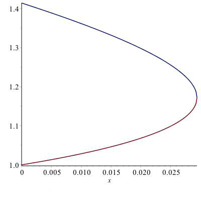
Figure 6: $\mu$ (bottom) and $\mu_{2}$ (top)

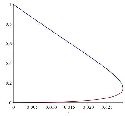
Figure 7: $\lambda$ (bottom) and $\lambda_{2}$ (top)

Lemma 21.

For $0<x<c_{0}$, we have $\mu(x)>1$, $\mu_{2}(x)>1$, $0<\lambda(x)<1$, and $0<\lambda_{2}(x)<1$.

Proof.

Elementary inequalities. ∎

Lemma 22.

As $x\to 0^{+}$,

$$\mu(x)\;{}_{2}F_{1}\left(\frac{1}{3},\frac{2}{3};1;\lambda(x)\right) =1+\frac{5}{2}\,x+O(x^{2}),$$

$$\mu_{2}(x)\;{}_{2}F_{1}\left(\frac{1}{3},\frac{2}{3};1;\lambda_{2}(x)\right) =\frac{-\sqrt{3}}{\pi\sqrt{2}}\,\log x+o(1).$$

The second one indeed has constant term zero.

Proof. Compute (as $z\to 0$ and $x\to 0$):

$$\mu(x) =1+\frac{5}{2}x+O(x^{2})$$

$$\lambda(x) =27x^{2}+O(x^{3})$$

$${}_{2}F_{1}\left(\frac{1}{3},\frac{2}{3};1;z\right) =1+\frac{2}{9}z+O(z^{2})$$

$${}_{2}F_{1}\left(\frac{1}{3},\frac{2}{3};1;\lambda(x)\right) =1+6x^{2}+O(x^{3})$$

$$\mu(x)\;{}_{2}F_{1}\left(\frac{1}{3},\frac{2}{3};1;\lambda(x)\right) =1+\frac{5}{2}x+O(x^{2})$$

For the second one, we apply Lemma 18(c). As $x\to 0$:

$$\mu_{2}(x) =\sqrt{2}-\frac{7}{\sqrt{2}}x+O(x^{2})$$

$$\lambda_{2}(x) =1-27x+O(x^{2})$$

$${}_{2}F_{1}\left(\frac{1}{3},\frac{2}{3};1;\lambda_{2}(x)\right) =-\frac{\sqrt{3}}{2\pi}\log(27x)+\frac{3\sqrt{3}\log 3}{2\pi}+o(1)$$

$$=-\frac{\sqrt{3}}{2\pi}(\log 27+\log x)+\frac{3\sqrt{3}\log 3}{2\pi}+o(1)$$

$$=-\frac{\sqrt{3}}{2\pi}\log x+o(1)$$

$$\mu_{2}(x){}_{2}F_{1}\left(\frac{1}{3},\frac{2}{3};1;\lambda_{2}(x)\right) =-\frac{\sqrt{3}}{\sqrt{2}\,\pi}\log x+o(1)\qquad\qed$$

Proposition 23.

$$u_{0}(x) =\mu(x)^{2}\;{}_{2}F_{1}\left(\frac{1}{3},\frac{2}{3};1;\lambda(x)\right)^{2},$$

$$v_{0}(x) =-\frac{2\pi}{\sqrt{3}(x+1)}\;{}_{2}F_{1}\left(\frac{1}{3},\frac{2}{3};1;\lambda(x)\right)\;{}_{2}F_{1}\left(\frac{1}{3},\frac{2}{3};1;\lambda_{2}(x)\right),$$

$$u_{\infty}(z) =\frac{1}{z}\mu\left(\frac{1}{z}\right)^{2}{}_{2}F_{1}\left(\frac{1}{3},\frac{2}{3};1;\lambda\left(\frac{1}{z}\right)\right)^{2}.$$

Proof.

Note: $\mu(x)\mu_{2}(x)=\sqrt{2}/(x+1)$. Verify that these expressions satisfy (The Differential Equation) as usual. Then verify the asymptotics using Lemma 22. ∎

How were these formulas found? The first one is from Mark van Hoeij [12, A005259]; I do not know how he found it. But then it is natural to try the other square root, since that will still satisfy the same differential equation.

Proposition 24.

$v_{0}(x)<0$ for $0<x<c_{0}$.

Proof.

For $0<x<c_{0}$: By Lemma 21, $0<\lambda(x)<1$, so by Lemma 18(b), $\;{}_{2}F_{1}\left(\frac{1}{3},\frac{2}{3};1;\lambda(x)\right)>0$. Similarly, $\;{}_{2}F_{1}\left(\frac{1}{3},\frac{2}{3};1;\lambda_{2}(x)\right)>0$. ∎

The Two Endpoints

Proposition 25.

On interval $(c_{0},c)$ we have exactly

$$\varphi(x)=\frac{v_{2}(x)}{2^{5/4}(\sqrt{2}+1)^{4}\pi^{2}}.$$

Proof.

We examine the solution $u_{\infty}(x)$ of (The Differential Equation) on the interval $(c,+\infty)$. As $\delta\to 0^{+}$, the Frobenius series solution shows that

$$u_{\infty}(c+\delta)=A+B\sqrt{\delta}+C\delta+O(\delta^{3/2})$$ (5)

for some real constants $A,B,C$; we will have to evaluate the constant $B$ below. Following (5) around the point $c$ by a half-turn in either direction, we get

$$u_{\infty}(c-\delta-i0) =A+B(-i)\sqrt{\delta}-C\delta+O(\delta^{3/2})$$

$$u_{\infty}(c-\delta+i0) =A+Bi\sqrt{\delta}-C\delta+O(\delta^{3/2})$$

$$\varphi(c-\delta) =\frac{1}{2\pi i}\big{(}u_{\infty}(c-\delta-i0)-u_{\infty}(c-\delta+i0)\big{)}$$

$$=\frac{0A-2Bi\sqrt{\delta}+0C\delta}{2\pi i}+O(\delta^{3/2})$$

$$=\frac{-B}{\pi}\sqrt{\delta}+O(\delta^{3/2}).$$

Therefore $\varphi(x)=(-B/\pi)v_{2}(x)$ on $(c_{0},c)$.

On interval $(c,+\infty)$, we have

$$u_{\infty}(x)=\frac{1}{x}\mu\left(\frac{1}{x}\right)^{2}{}_{2}F_{1}\left(\frac{1}{3},\frac{2}{3};1;\lambda\left(\frac{1}{x}\right)\right)^{2}.$$

The value $\lambda(1/x)$ stays inside the unit disk, so no analytic continuation is required. Now $\lambda(c_{0})=\lambda_{2}(c_{0})=1/(2^{3/2}(\sqrt{2}+1))$, called $z_{0}$ in Lemma 19. Let $S_{0},S_{1}$ also be as in Lemma 19. As $\delta\to 0^{+}$,

$$\frac{1}{c+\delta} =\frac{1}{(\sqrt{2}+1)^{4}}+O(\delta)$$

$$\mu\left(\frac{1}{c+\delta}\right) =\frac{(\sqrt{2}+1)}{2^{1/4}3^{1/2}}-\frac{1}{4\cdot 3\cdot(\sqrt{2}+1)}\sqrt{\delta}+O(\delta)$$

$$\lambda\left(\frac{1}{c+\delta}\right) =\frac{1}{2^{3/2}(\sqrt{2}+1)}-\frac{\sqrt{3}}{2^{9/4}(\sqrt{2}+1)^{2}}\sqrt{\delta}+O(\delta)$$

$${}_{2}F_{1}\left(\frac{1}{3},\frac{2}{3};1;\lambda\left(\frac{1}{c+\delta}\right)\right) =S_{0}-\frac{\sqrt{3}}{2^{9/4}(\sqrt{2}+1)^{2}}S_{1}\sqrt{\delta}+O(\delta)$$

$$u_{\infty}(c+\delta) =\frac{S_{0}^{2}}{3\sqrt{2}(\sqrt{2}+1)^{2}}-\frac{S_{0}(3S_{1}+\sqrt{2}S_{0})}{2^{7/4}3^{3/2}(\sqrt{2}+1)^{4}}\sqrt{\delta}+O(\delta)$$

$$=\frac{S_{0}^{2}}{3\sqrt{2}(\sqrt{2}+1)^{2}}-\frac{1}{2^{5/4}(\sqrt{2}+1)^{4}\pi}\sqrt{\delta}+O(\delta).$$

So we get $B=-1/(2^{5/4}(\sqrt{2}+1)^{4}\pi)$. ∎

Proposition 26.

On interval $(0,c_{0})$ we have exactly $\varphi(x)=-6v_{0}(x)/\pi^{2}$.

Proof.

We examine the solution $u_{\infty}(x)$ of (The Differential Equation) on the interval $(-\infty,0)$. As $\delta\to 0^{+}$, the Frobenius series solution shows that

$$u_{\infty}(-\delta)=A+B\log\delta+C(\log\delta)^{2}+o(1)$$ (6)

for some real constants $A,B,C$; we will have to evaluate the constants $B$ and $C$ below. Following (6) around the point $0$ by a half-turn in either direction, we get

$$u_{\infty}(\delta-i0) =A+B(\log\delta+i\pi)+C(\log\delta+i\pi)^{2}+o(1)$$

$$u_{\infty}(\delta+i0) =A+B(\log\delta-i\pi)+C(\log\delta-i\pi)^{2}+o(1)$$

$$\varphi(\delta) =\frac{1}{2\pi i}\big{(}u_{\infty}(\delta-i0)-u_{\infty}(\delta+i0)\big{)}$$

$$=\frac{2Bi\pi+4Ci\pi\log\delta}{2\pi i}+o(1)$$

$$=B+2C\log\delta+o(1)$$

Therefore $\varphi(x)=Bu_{0}(x)+2Cv_{0}(x)$ on $(0,c_{0})$.

On interval $(-\infty,0)$, we have

$$u_{\infty}(x)=\frac{1}{x}\mu\left(\frac{1}{x}\right)^{2}{}_{2}F_{1}\left(\frac{1}{3},\frac{2}{3};1;\lambda\left(\frac{1}{x}\right)\right)^{2}.$$

Argument $\lambda(1/x)$ stays inside the unit disk, so this is an easy analytic continuation of $u_{\infty}$. As $\delta\to 0^{+}$,

$$\frac{1}{-\delta} =\frac{-1}{\delta}+O(1)$$

$$\mu\left(\frac{1}{-\delta}\right)^{2} =\delta+O(\delta^{2})$$

$$\lambda\left(\frac{1}{-\delta}\right) =1-27\delta^{2}+O(\delta^{3})$$

So by Lemma 18(c),

$${}_{2}F_{1}\left(\frac{1}{3},\frac{2}{3};1;\lambda\left(\frac{1}{-\delta}\right)\right) =\frac{-\sqrt{3}}{2\pi}\;2\log\delta+o(1)$$

$$u_{\infty}(-\delta) =\frac{-3}{\pi^{2}}(\log\delta)^{2}+o(1).$$

Thus we get $B=0$ and $C=-3/\pi^{2}$. ∎

Corollary 27.

The moment density $\varphi$ may be written

$$\varphi(x)=\begin{cases}\displaystyle\;\frac{-6}{\pi^{2}}\,v_{0}(x),&0<x<c_{0},\\ {}\\ \displaystyle\;\frac{1}{2^{5/4}(\sqrt{2}+1)^{4}\pi^{2}}\,v_{2}(x),&c_{0}\leq x\leq c.\end{cases}$$

It is positive on $(0,c_{0})\cup(c_{0},c)$.

Proof.

For $0<x<c_{0}$, by Prop. 24 $v_{0}(x)<0$. For $c_{0}<x<c$, by Prop. 16 $v_{2}(x)>0$. ∎

This completes the proof of Theorem 1.

Appendix: Lemma 19

Let the degree $1$ Taylor polynomial for ${}_{2}F_{1}\left(\frac{1}{3},\frac{2}{3};1;z\right)$ at $z_{0}=1/(2^{3/2}(1+\sqrt{2}\;))$ be ${}_{2}F_{1}\left(\frac{1}{3},\frac{2}{3};1;z\right)=S_{0}+S_{1}\cdot(z-z_{0})+o(|z-z_{0}|)$ as $z\to z_{0}$. Then

$$S_{0}\cdot(3S_{1}+\sqrt{2}S_{0})=\frac{3^{3/2}2^{1/2}}{\pi}.$$

We will see that a proof can be given using modular parameterizations. See [3, 6, 13].

Notation. Let $\tau$ be a complex variable with $\operatorname{Im}\tau>0$ and let $q=e^{2\pi i\tau}$ so that $0<|q|<1$. Thus

$$\frac{dq}{d\tau}=2\pi ie^{2\pi i\tau}=2\pi iq,\qquad\frac{d\tau}{dq}=\frac{1}{2\pi iq}.$$

We will use a derivation $\boldsymbol{\theta}$ defined by

$$\boldsymbol{\theta}=q\;\frac{d}{dq}=\frac{1}{2\pi i}\;\frac{d}{d\tau}.$$

Sometimes this derivative will be written as a superscript:

$$q\frac{d}{dq}f=\frac{1}{2\pi i}\;\frac{d}{d\tau}f=\boldsymbol{\theta}f=f^{\boldsymbol{\theta}}(\tau).$$

We will use the following functions: The Dedekind eta function,

$$\eta=q^{1/24}\prod_{n=1}^{\infty}(1-q^{n}).$$ (7)

One of the McKay-Thompson modular functions [12, A030182]

$$j_{3B}(\tau) =\frac{\eta(\tau)^{12}}{\eta(3\tau)^{12}}$$

$$=q^{-1}-12+54q-76q^{2}-243q^{3}+1188q^{4}-1384q^{5}$$

$$\qquad\qquad-2916q^{6}+11934q^{7}-11580q^{8}-21870q^{9}+\dots$$

And: the Eisenstein series $E_{2}$; the logarithmic derivative of $\eta^{24}$, in the sense

$$E_{2}=24\;\frac{\eta^{\boldsymbol{\theta}}}{\,\eta\,}.$$

The Fourier series is [12, A006352]

$$E_{2}=1-24\sum_{k=1}^{\infty}\sigma(k)q^{k},$$

where the number-theoretic function $\sigma(k)$ is the sum of the (positive integer) divisors of $k$. This is from logarithmic differentiation of $(\ref{etaprod})$.

Logarithmic differentiation of $j_{3B}$ yields

$$\frac{j^{\boldsymbol{\theta}}_{3B}(\tau)}{j_{3B}(\tau)}=\frac{1}{2}E_{2}(\tau)-\frac{3}{2}E_{2}(3\tau).$$

Our calculations will require values of $\eta$ and $E_{2}$ for $\tau=i\sqrt{6}$ and $i\sqrt{6}/3$. These values may be written in terms of the constant

$$\mathbf{K}:={}_{2}F_{1}\left(\frac{1}{6},\frac{1}{3};1;\frac{1}{2}\right)\approx 1.0354935.$$

In fact,

$$\mathbf{K}=\frac{3^{1/4}\sqrt{2}}{8\pi^{3/2}}\sqrt{\Gamma\left(\frac{1}{24}\right)\Gamma\left(\frac{5}{24}\right)\Gamma\left(\frac{7}{24}\right)\Gamma\left(\frac{11}{24}\right)},$$

but we will not need this value for the proof of Lemma 19.

For evaluation at $\tau=i\sqrt{6}/3$, we will use these values:

$$\tau =\frac{i\sqrt{6}}{3}$$

$$3\tau =i\sqrt{6}$$

$$\eta(\tau) =\frac{2^{3/4}3^{7/8}(1+\sqrt{2}\;)^{1/12}\mathbf{K}^{1/2}}{6}$$

$$\eta(3\tau) =\frac{2^{3/4}3^{5/8}(\sqrt{2}-1)^{1/12}\mathbf{K}^{1/2}}{6}$$

$$E_{2}(\tau) =\frac{3\sqrt{6}}{2\pi}+\frac{(\sqrt{2}+1)\mathbf{K}^{2}}{\sqrt{2}}$$

$$E_{2}(3\tau) =\frac{\sqrt{6}}{2\pi}+\frac{(\sqrt{2}+1)\mathbf{K}^{2}}{3\sqrt{2}}$$

$$j_{3B}(\tau) =27(1+\sqrt{2}\;)^{2}$$

$$\frac{27}{j_{3B}(\tau)+27} =\frac{1}{2}-\frac{\sqrt{2}}{4}=z_{0}$$

$$j_{3B}^{\boldsymbol{\theta}}(\tau) =27(1+\sqrt{2}\;)^{2}\mathbf{K}^{2}.$$

Begin with this modular parameterization for ${}_{2}F_{1}(\frac{1}{3},\frac{2}{3};1;z)$:

$${}_{2}F_{1}\left(\frac{1}{3},\frac{2}{3};1;\frac{27}{j_{3B}(\tau)+27}\right)=\frac{\eta(3\tau)^{3}}{\eta(\tau)}\;(j_{3B}(\tau)+27)^{1/3}.$$ (8)

This is proved using a standard method: Each side is a modular form of weight $2$ and level $3$. The space of such modular forms is finite-dimensional, so it suffices to check that a certain number of the Fourier coefficients agree.

Write $F(z)={}_{2}F_{1}(\frac{1}{3},\frac{2}{3};1;z)$. That means $S_{0}=F(z_{0})$ and $S_{1}=F^{\prime}(z_{0})$. Substitution of $\tau=i\sqrt{6}/3$ into (8) yields

$$S_{0}=\mathbf{K}.$$ (9)

Logarithmic differentiation of (8) yields

$$-\frac{27}{2}\frac{\eta(\tau)}{\eta(\tau)^{3}}j_{3B}^{\boldsymbol{\theta}}(\tau)(E_{2}(\tau)-3E_{2}(3\tau))\frac{j_{3B}(\tau)}{(j_{3B}(\tau)+27)^{1/3}}F^{\prime}\left(\frac{27}{j_{3B}(\tau)+27}\right)$$

$$=\frac{9E_{2}(3\tau)-E_{2}(\tau)}{24}+\frac{E_{2}(\tau)-3E_{2}(3\tau)}{6}\frac{j_{3B}(\tau)}{j_{3B}(\tau)+27}$$ .

Substitution of $\tau=i\sqrt{6}/3$ yields

$$\frac{\mathbf{K}}{8}F^{\prime}(z_{0})=\frac{\sqrt{6}}{8\pi}-\frac{\sqrt{2}\mathbf{K}^{2}}{24},$$

so

$$S_{1}=\frac{\sqrt{6}}{\pi\mathbf{K}}-\frac{\sqrt{2}\mathbf{K}}{3}.$$ (10)

Finally, from (9) and (10) we obtain

$$S_{0}\;(3S_{1}+\sqrt{2}\;S_{0})=\frac{3\sqrt{6}}{\pi}$$

as claimed.