Graphical continuous Lyapunov models

Abstract

The linear Lyapunov equation of a covariance matrix parametrizes the equilibrium covariance matrix of a stochastic process. This parametrization can be interpreted as a new graphical model class, and we show how the model class behaves under marginalization and introduce a method for structure learning via $\ell_{1}$-penalized loss minimization. Our proposed method is demonstrated to outperform alternative structure learning algorithms in a simulation study, and we illustrate its application for protein phosphorylation network reconstruction.

1 INTRODUCTION

Path analysis as introduced by Wright (1921, 1934) illustrates how covariance computations in linear models can benefit from a graphical model representation. Today there is a vast literature on linear structural equation models and their corresponding algebraic and graphical model theory, see e.g. Drton (2018). Within this framework, the standard parametrization specifies the covariance matrix $\Sigma$ as a solution to the equation

$$(I-\Lambda)^{T}\Sigma(I-\Lambda)=\Omega$$ (1)

for matrix parameters $\Lambda$ and $\Omega$. The associated mixed graph has directed edges and bidirected edges determined by the nonzero entries of $\Lambda$ and $\Omega$, respectively. If we fix an acyclic graph, say, the framework provides a parametrization of the observables from a directed acyclic model – potentially with latent variables – see (Richardson and Spirtes, 2002). In the cyclic case the parametrization can, moreover, be interpreted as an equilibrium distribution for a deterministic process whenever the spectrum of $\Lambda$ is inside the unit circle, see e.g. (Hyttinen et al., 2012).

It is, however, well known that for certain continuous time stochastic processes the equilibrium covariance matrix does not have a simple graphical representation using the parametrization above, see e.g. (Mogensen et al., 2018). Instead it has an alternative parametrization corresponding to the graphical representation of the dynamics of the process. In this parametrization, $\Sigma$ is the solution to the continuous Lyapunov equation,

$$B\Sigma+\Sigma B^{T}+C=0$$ (2)

where $B$ and $C$ are matrices parametrizing $\Sigma$.

Models given by (2) are of practical interest when only cross-sectional data from the stochastic process can be obtained. This is the case for biological systems such as gene regulatory or protein signalling networks, where cells are destroyed in the measurement process. Existing methods based on correlation or mutual information, such as the ARACNe method by Basso et al. (2005), the use of directed graphical models, (Sachs et al., 2005), or the graphical lasso giving undirected graphs, (Friedman et al., 2007), cannot represent feedback processes, whereas cycles can be encoded naturally by (2).

The main objective of this paper is to develop the framework of graphical models parametrized by (2) and to introduce a learning algorithm of the graphical structure. In the preparation of this paper we found that similar ideas were recently considered by Young et al. (2019) and Fitch (2019). The work by Fitch (2019) is based on (2) and a learning algorithm was proposed, while Young et al. (2019) considered the vector autoregressive model, whose equilibrium covariance matrix solves the discrete Lyapunov equation.

We connect in this paper the models parametrized by (2) to the concept of local independence for stochastic processes, and we present new results about these models as graphical models. To this end, recall that Wright’s path analysis lead to polynomial expressions of the entries in $\Sigma$ in terms of the nonzero entries in $\Lambda$ and $\Omega$. Such formulas are in modern terminology known as trek rules, and they explain how graphical structural constraints are encoded into $\Sigma$. By introducing trek seperation, Sullivant et al. (2010) gave, for instance, a complete graph-theoretic characterization in the acyclic case of when submatrices of $\Sigma$ will drop rank. Another example is the half-trek criterion for generic identifiability by Foygel et al. (2012).

In this paper we associate a mixed graph to the covariance matrix solving (2) and establish a version of trek rules when $B$ is a stable matrix. We use this to introduce a novel graphical projection yielding a parametrization of marginalized models in terms of solutions to Lyapunov equations. To fit models parametrized by (2), but with an unknown graphical structure, we propose $\ell_{1}$-penalized loss minimization using either the Frobenius norm or the Gaussian log-likelihood loss. They outperformed the learning algorithm proposed by Fitch (2019) in a simulation study, and we illustrate the use of the method for protein phosphorylation network discovery using data from Sachs et al. (2005).

2 GRAPHICAL CONTINUOUS LYAPUNOV MODELS

We will consider models of covariance matrices determined as solutions to the Lyapunov equation (2) and parametrized by the matrices $B$ and $C$. Note that (2) can be written in tensor product form as the linear equation

$$(B\otimes I+I\otimes B)\mathrm{vec}(\Sigma)=-\mathrm{vec}(C).$$

The eigenvalues of the kronecker sum $B\otimes I+I\otimes B$ are sums of pairs of eigenvalues of $B$, (Horn and Johnson, 1991, Theorem 4.4.5). The solution to (2) is thus unique if and only if the sum of any two eigenvalues of $B$ is nonzero, in which case $\Sigma(B,C)$ will denote the unique solution.

Some notation and terminology is needed to study solutions of (2). Introduce $\mathrm{Mat}_{0}(p)$ as the set of $p\times p$ matrices that do not have two eigenvalues summing to zero, and let $\mathrm{Sym}(p)$ denote the set of symmetric $p\times p$ matrices. Let $\mathrm{Stab}(p)$ denote the set of stable $p\times p$ matrices, that is, matrices whose eigenvalues all have a strictly negative real part. Obviously, $\mathrm{Stab}(p)\subseteq\mathrm{Mat}_{0}(p)$. The set of $p\times p$ positive definite matrices is denoted $\mathrm{PD}(p)$.

The sparsity patterns of the parameters $B$ and $C$ will be encoded via a mixed graph, that is, a graph $\mathcal{G}=([p],E)$ with vertices $[p]=\{1,\ldots,p\}$ and with $E$ containing directed as well as bidirected edges. Self loops and multiple edges between two nodes are allowed. We say that a pair of matrices $(B,C)\in\mathrm{Mat}_{0}(p)\times\mathrm{Sym}(p)$ are compatible with a mixed graph $\mathcal{G}$ if $B_{ji}\neq 0$ implies $i\rightarrow j$ and $C_{ij}\neq 0$ implies $i\leftrightarrow j$. The set of $\mathcal{G}$-compatible matrix pairs is denoted $\Xi_{\mathcal{G}}\subseteq\mathrm{Mat}_{0}(p)\times\mathrm{Sym}(p)$, and $\Theta_{\mathcal{G}}=\Xi_{\mathcal{G}}\cap\left(\mathrm{Stab}(p)\times\mathrm{PD}(p)\right).$

Given a mixed graph $\mathcal{G}$, the map $(B,C)\mapsto\Sigma(B,C)$ is well defined on $\Xi_{\mathcal{G}}$ with image in $\mathrm{Sym}(p)$. The restriction of this map to $\Theta_{\mathcal{G}}$ has image in $\mathrm{PD}(p)$, which follows from Proposition 2.1 below. Let $\mathcal{M}_{\mathcal{G}}=\Sigma(\Theta_{\mathcal{G}})\subseteq\mathrm{PD}(p)$ denote the image of $\Theta_{\mathcal{G}}$, which we call the graphical continuous Lyapunov model (GCLM) with graph $\mathcal{G}$. The extended GCLM is $\mathcal{M}_{\mathcal{G}}^{e}=\Sigma(\Xi_{\mathcal{G}})$.

2.1 STOCHASTIC PROCESSES AND LOCAL INDEPENDENCE

To motivate (2) consider the $p$-dimensional Ornstein-Uhlenbeck process given as a solution to the stochastic differential equation

$$dX_{t}=B(X_{t}-a)dt+DdW_{t}$$ (3)

where $B$ and $D$ are $p\times p$ matrices, $a\in\mathbb{R}^{p}$ and $W_{t}$ is a standard Brownian motion in $\mathbb{R}^{p}$. If $B$ is a stable matrix, (3) has a Gaussian equilibrium distribution with covariance matrix $\Sigma(B,DD^{T})$, see e.g. (Jacobsen, 1991, Theorem 2.12). Thus solutions of (2) arise as equilibrium covariances for continuous time stochastic processes.

We call (3) a structural causal stochastic differential equation if it adequately captures effects of interventions, see (Sokol and Hansen, 2014). In this case the directed part of the mixed graph $\mathcal{G}$ – introduced above in terms of $B$ – represents direct causal effects. Moreover, if there is no directed edge from $i$ to $j$, the corresponding coordinates of the stochastic process satisfy an infinitesimal conditional independence, and we say that $X_{t}^{j}$ is locally independent of $X_{t}^{i}$. The directed part of $\mathcal{G}$ is, by Definition 12 in Mogensen et al. (2018), also identical to the local independence graph determined by (3).

If $C=DD^{T}$ is diagonal, the local independence graph has the global Markov property for local independence, see Mogensen et al. (2018), who also gave a learning algorithm for partially observed systems. That general algorithm learns an equivalence class of local independence graphs by local independence queries. In the specific case of solutions to (3), the equilibrium covariance matrix also carries information about the local independence graph as encoded via the Lyapunov equation. As we will show below, graphical representations of the marginalization of the equilibrium covariance matrix requires a new graphical projection that introduces additional bidirected edges, but in any case, at least for diagonal $C$, the directed edges of $\mathcal{G}$ have an interpretation as local dependences – and even direct causal effects if (3) is a structural causal stochastic differential equation.

2.2 TREKS

To obtain a graphical representation of $\Sigma=\Sigma(B,C)\in\mathcal{M}_{\mathcal{G}}$ for a mixed graph $\mathcal{G}$ we introduce

$$\Sigma(s)=\int_{0}^{s}e^{uB}Ce^{uB^{T}}\mathrm{d}u.$$ (4)

The following is a well known result, see (Jacobsen, 1991) or (Fitch, 2019, Theorem 2), but we include it for completeness.

Proposition 2.1.

For $(B,C)\in\Theta_{\mathcal{G}}$

$$\Sigma(B,C)=\lim_{s\to\infty}\Sigma(s)=\int_{0}^{\infty}e^{uB}Ce^{uB^{T}}\mathrm{d}u.$$ (5)

Proof.

First note that stability of $B$ ensures that the solution to the Lyapunov equation is unique. It also ensures that the integral in (5) is convergent. We see that if $\Sigma$ is given by the r.h.s. of (5) then

$$B\Sigma+\Sigma B^{T} =\int_{0}^{\infty}Be^{uB}Ce^{uB^{T}}+e^{uB}Ce^{uB^{T}}B^{T}\mathrm{d}u$$

$$=\int_{0}^{\infty}\frac{\mathrm{d}}{\mathrm{d}u}e^{uB}Ce^{uB^{T}}\mathrm{d}u=-C,$$

which shows that $\Sigma$ solves (2). ∎

The representation (5) implies that $\Sigma$ is positive definite if $C$ is, which shows that $\mathcal{M}_{\mathcal{G}}\subseteq\mathrm{PD}(p)$ as claimed above.

A trek from $i$ to $j$, denoted $i\leadsto j$, is a walk of the form

$$\tau:\ \underbrace{i\leftarrow\cdots\leftarrow i_{1}}_{n(\tau)}\leftarrow k\leftrightarrow l\rightarrow\underbrace{j_{1}\rightarrow\cdots\rightarrow j}_{m(\tau)}$$

where $k,l\in[p]$ are connected by a bidirected edge. Thus a trek consists of a left hand side, which is a directed walk $k\rightarrow i_{1}\rightarrow\ldots\rightarrow i$ of length $n(\tau)$, and a right hand side, which is a directed walk $l\rightarrow j_{1}\rightarrow\ldots\rightarrow j$ of length $m(\tau)$. Those two walks are connected by the bidirected edge $k\leftrightarrow l$. For every trek $i\leadsto j$ there is a reversed trek, $j\leadsto i$, corresponding to interchanging the roles of the left and right hand sides of the trek. Note that $n(\tau)=0$ with $i=k$ as well as $m(\tau)=0$ with $j=l$ are allowed. Define also

$$\kappa(s,\tau)=\frac{s^{(n(\tau)+m(\tau)+1)}}{(n(\tau)+m(\tau)+1)n(\tau)!m(\tau)!}$$

for any trek $\tau$ and $s\in\mathbb{R}$, and introduce for $(B,C)\in\Theta_{\mathcal{G}}$ and a trek $\tau$ the trek weight

$$\omega(B,C,\tau)=C_{k,l}\prod_{g\rightarrow h\in\tau}B_{hg}.$$

Proposition 2.2.

For $(B,C)\in\Theta_{\mathcal{G}}$

$$\Sigma(s)_{ij}=\sum_{\tau\in\mathcal{T}(i,j)}\kappa(s,\tau)\omega(B,C,\tau)$$

where $\mathcal{T}(i,j)$ denotes the set of all treks from $i$ to $j$.

Proof.

Using the series expansion of the matrix exponential we find that

$$\Sigma(s)_{ij} =\int_{0}^{s}\sum_{n=0}^{\infty}\sum_{m=0}^{\infty}\sum_{k,l=1}^{p}\frac{t^{n}t^{m}}{n!m!}(B^{n})_{ik}C_{kl}(B^{m})_{jl}\mathrm{d}t$$

$$=\sum_{n=0}^{\infty}\sum_{m=0}^{\infty}\sum_{k,l=1}^{p}\frac{s^{(n+m+1)}}{(n+m+1)n!m!}(B^{n})_{ik}C_{kl}(B^{m})_{jl}$$

$$=\sum_{\tau\in\mathcal{T}(i,j)}\kappa(s,\tau)\omega(B,C,\tau).\qed$$

The following corollary is an immediate consequence of Propositions 2.1 and 2.2.

Corollary 2.3.

If $\Sigma\in\mathcal{M}_{\mathcal{G}}$ and there is no trek from $i$ to $j$ in $\mathcal{G}$ then $\Sigma_{ij}=0$.

2.3 MARGINALIZATION

Let $\Sigma$ be a $p^{\prime}\times p^{\prime}$ matrix that solves the Lyapunov equation for given $B$ and $C$, and suppose that we only observe variables corresponding to the top left $p\times p$ block, $\Sigma_{11}$, for $p<p^{\prime}$. Writing out the Lyapunov equation in block matrix form gives four coupled equations. The one corresponding to $\Sigma_{11}$ is the Lyapunov equation

$$B_{11}\Sigma_{11}+\Sigma_{11}B_{11}^{T}+\tilde{C}=0$$ (6)

with $\tilde{C}=B_{12}\Sigma_{21}+\Sigma_{12}B_{12}^{T}+C_{11}.$

When $C$ is symmetric so is $\tilde{C}$, but there is no guarantee that it is positive definite even if $C$ is so, nor that $B_{11}$ is stable if $B$ is so. What we can show is that if $\Sigma$ is a GCLM then $\Sigma_{11}$ is an extended GCLM. To do so we will introduce a graphical projection map.

For $\mathcal{G}=([p^{\prime}],E)$ a mixed graph let $\mathcal{G}[p]=([p],E[p])$ denote the projection onto the first $p<p^{\prime}$ vertices defined as follows: for $i,j\in[p]$

• $i\rightarrow j\in E[p]$ if $i\rightarrow j\in E$

• $i\leftrightarrow j\in E[p]$ if $i\leftrightarrow j\in E$

• $i\leftrightarrow j\in E[p]$ if for some $k>p$ there is a trek from $i$ to $j$ of the forms $i\leftarrow k\leadsto j$ or $i\leadsto k\rightarrow j$

Thus the projected graph retains all edges in $\mathcal{G}$ between vertices in $[p]$. In addition, it has bidirected edges between vertices $i,j\in[p]$ that are connected by a trek containing a vertex not in $[p]$, which is directly connected to either $i$ or $j$ in the trek. It should be noted that this is not a standard latent graph projection. For once, only bidirected arrows are added.

Proposition 2.4.

If $\Sigma\in\mathcal{M}_{\mathcal{G}}$ and $B_{11}\in\mathrm{Mat}_{0}$ then $\Sigma_{11}\in\mathcal{M}^{e}_{\mathcal{G}[p]}$.

Proof.

It is clear from the definitions that $B_{11}$ fulfills the $\mathcal{G}[p]$-compatibility requirement. Observe then that

$$\tilde{C}_{ij}=C_{ij}+\sum_{k=p+1}^{p^{\prime}}\left(B_{ik}\Sigma_{kj}+\Sigma_{ik}B_{jk}\right),$$

which is symmetric in $i$ and $j$. If $C_{ij}\neq 0$ then $i\leftrightarrow j$. If $\tilde{C}_{ij}\neq 0$, but $C_{ij}=0$, then there is a $k>p$ such that $B_{ik}\Sigma_{kj}\neq 0$ or $\Sigma_{ik}B_{jk}\neq 0$. In the first case this means that $\Sigma_{kj}\neq 0$, and by Corollary 2.3 there is a trek from $k$ to $j$. Now as $B_{ik}\neq 0$ as well, we can extend the trek to the left with the edge $k\to i$, and $i\leftrightarrow j$ by the definition of $\mathcal{G}[p]$. A similar argument applies if $\Sigma_{ik}B_{jk}\neq 0$.

In conclusion, $(B_{11},\tilde{C})$ is $\mathcal{G}[p]$-compatible, and since it is assumed that $B_{11}\in\mathrm{Mat}_{0}$ we have that

$$\Sigma_{11}=\Sigma(B_{11},\tilde{C})\in\mathcal{M}^{e}_{\mathcal{G}[p]}.\qed$$

Figure 1: Mixed graphs representing a GCLM with $p=5$ nodes (A) and the extended GCLM (B) obtained by marginalization of (A). The larger model (A) has $C=I$ and the nonzero entries of $B$ are shown as edge weights for the directed edges. The marginalized model (B) has the same directed edge weights and the nonzero entries of $\tilde{C}$ are shown as edge weights for the bidirected edges.

2.4 EXAMPLE

Consider the GCLM with $\mathcal{G}$ as given by (A) in Figure 1. In this example $p=5$ and the only bidirected edges are self loops. The directed part of $\mathcal{G}$ is the local independence graph of the stochastic process, see Section 2.1.

The specific model has

$${B=\left(\begin{array}[]{rrrrr}-1&1&.&.&.\\ -1&.&0.2&.&.\\ .&.&-1&-0.5&.\\ .&.&.&-1&1\\ .&.&1&.&-1\\ \end{array}\right)}$$

and $C=I_{5}$ the identity matrix. The eigenvalues of $B$ are

$$-1.79,\ -0.60\pm 0.69i,\text{ and }-0.50\pm 0.87i,$$

with all real parts strictly negative, whence $B$ is stable. The graphical projection when projecting away node 5 is shown in Figure 1 (B). The only directed edge out of 5 is $5\rightarrow 4$, and it follows from the projection map that the added bidirected edges are $4\leftrightarrow 1$, $4\leftrightarrow 2$ and $4\leftrightarrow 3$. In this example, $B_{11}$ is, in fact, still a stable matrix, and by solving the Lyapunov equation in terms of $B$ and $C$ the $\tilde{C}$ matrix was computed to be

$${\tilde{C}=\left(\begin{array}[]{rrrr}1&.&.&0.05\\ .&1&.&0.07\\ .&.&1&0.20\\ 0.05&0.07&0.20&1.60\\ \end{array}\right).}$$

The graphical projection in Figure 1 (B) should be compared to the graphical projection of the local independence graph, (Mogensen and Hansen, 2020; Mogensen et al., 2018), which introduces a directed edge from node 3 to node 4 instead of the three bidirected edges. That projection represents local independences of the marginalized nodes (Mogensen and Hansen, 2020). We have not developed a notion of separation for the mixed graph in Figure 1 (B), and it does not represent local independence among the marginalized nodes directly. However, its representation of the parametrization of the marginalized equilibrium covariance matrix allows us to read of direct causal effects among the observed nodes when the model of all nodes is a structural causal stochastic differential equation.

3 STRUCTURE RECOVERY

We propose minimizing an $\ell_{1}$-penalized loss to estimate the directed part of a GCLM as given by the $B$ matrix in 2. The $C$ matrix will be held diagonal.

Specifically, we suggest estimating $(B,C)$ by solving the following optimization problem for a generic differentiable loss function $L:\mathrm{PD}(p)\to\mathbb{R}$:

$$\begin{array}[]{ll}\text{minimize}&L\left(\Sigma(B,C)\right)+\lambda\rho_{1}(B)+\kappa||C-I_{p}||_{F}^{2}\\ \text{subject to}&B\text{ stable and }C\text{ diagonal},\end{array}$$ (7)

where $\lambda,\kappa\geq 0$ are regularization parameters and $\rho_{1}(B)=\sum_{i\neq j}|B_{ij}|$ is the $1$-norm of the off-diagonal entries of $B$. The penalization term involving the Frobenius norm of the difference between $C$ and the identity matrix is necessary, since the pair $(B,C)$ can only be identified up to a multiplicative constant. Letting $\kappa=+\infty$, we obtain as a special case an estimator of $B$ with $C=I_{p}$ fixed. Smaller values of $\kappa$ allow for $C$ matrices with diverging diagonal entries.

Examples of loss functions are the negative Gaussian log-likelihood

$$\log\det\Sigma+\operatorname{tr}\left(\hat{\Sigma}\Sigma^{-1}\right),$$

and the squared Frobenius loss

$$\|\Sigma-\hat{\Sigma}\|_{F}^{2}=\sum_{i,j}\left(\Sigma_{ij}-\hat{\Sigma}_{ij}\right)^{2},$$

for a given positive semi-definite matrix $\hat{\Sigma}$.

We use a variation of the proximal gradient algorithm for solving (7), see  (Parikh and Boyd, 2014), even though the optimization problem is in general non-convex. The proximal operator for $\ell_{1}$-penalization is soft-thresholding ($\mathcal{S}_{t}(x)=\operatorname{sign}(x)\left(|x|-t\right)$), and each iteration of the algorithm amounts to

$$C^{(k)} =C^{(k-1)}-st\kappa(C^{(k-1)}-I_{p})$$

$$-st(\nabla_{C}L(\Sigma(B^{(k-1)},C^{(k-1)})))$$

$$B^{(k)} =\mathcal{S}_{sr\lambda}\left(B^{(k-1)}-sr\nabla_{B}L(\Sigma(B^{(k-1)},C^{(k-1})))\right),$$

where soft-thresholding of a matrix is defined elementwisely. The global step size $s$ is chosen using line search as in Beck and Tabulle (2010) once the independent steps $t$ and $r$ have been chosen small enough that $C^{(k)}$ is positive definite and $B^{(k)}$ is stable.

Detailed pseudo-code of our proposed proximal gradient based algorithm is given as Algorithm 1.

The gradients with respect to $B$ and $C$ can be obtained with the cost of solving one additional Lyapunov equation as shown in the following proposition.

Proposition 3.1.

The gradient of $L(\Sigma(B,C))$ with respect to $(B,C)$ can be computed as follows,

$$\nabla_{B}(L(\Sigma(B,C))) =2\Sigma(B,C)\Sigma(B^{t},\nabla L),$$

$$\nabla_{C}(L(\Sigma(B,C))) =2\Sigma(B^{t},\nabla L),$$

where $\nabla L$ denotes the gradient of $\Sigma\mapsto L(\Sigma)$.

Proof.

Similar to Malagò et al. (2018) we differentiate the Lyapunov equation and we obtain:

$$B\frac{\partial\Sigma(B,C)}{\partial B_{ij}}+\frac{\partial\Sigma(B,C)}{\partial B_{ij}}B^{t}+Q_{(i,j)}(B,C)=0,$$

$$Q_{(i,j)}(B,C)=E_{(i,j)}\Sigma(B,C)+\Sigma(B,C)E_{(j,i)},$$

where $\left(E_{(i,j)}\right)_{kl}=\delta_{ik}\delta_{jl}$ with $\delta_{ij}$ the usual Kronecker delta. The Jacobian components are thus solutions of Lyapunov equations,

$$\frac{\partial\Sigma(B,C)}{\partial B_{i,j}}=\Sigma\left(B,Q_{(i,j)}(B,C)\right).$$ (8)

Thanks to (8) we can compute the gradient of any function, which is a composition of $\Sigma(B,C)$ and a differentiable function over the cone of positive definite matrices $L:\mathrm{PD}(p)\to\mathbb{R}$, as

$$\frac{\partial L\left(\Sigma(B,C)\right)}{\partial B_{ij}}=\operatorname{tr}\left(\Sigma(B,Q_{(i,j)})\frac{\partial L(\Sigma(B,C))}{\partial\Sigma}\right).$$ (9)

We note now that, for fixed stable $B$, $\Sigma(B,\cdot)$ is a linear operator on the symmetric matrices with adjoint operator given by $\Sigma(B^{t},\cdot)$ (Bhatia, 1997). That is,

$$\operatorname{tr}\left(\Sigma(B,C)D\right)=\operatorname{tr}\left(C\Sigma(B^{t},D)\right).$$

Thus from (9) we obtain the desired expression for the gradient,

$$\frac{\partial L\left(\Sigma(B,C)\right)}{\partial B_{ij}}= \operatorname{tr}\left(Q_{(i,j)}\Sigma\left(B^{t},\nabla L\right)\right)$$

$$= \left(2\Sigma(B,C)\Sigma(B^{t},\nabla L)\right)_{ij}.$$

The formula for $\nabla_{C}(L(\Sigma(B,C)))$ can be obtained analogously. ∎

Algorithm 1 Proximal gradient algorithm for minimization of $\ell_{1}$-penalized loss

0:  $L:\mathrm{PD}(p)\to\mathbb{R}\text{ differentiable}$,     $B_{0}\in\mathrm{Stab}(p)$,     $M\in\mathbb{N}$, $\varepsilon,\lambda,\kappa>0,\alpha\in(0,1)$

1:  $B=B_{0}$, $C=I_{p}$

2:  $\Sigma=\Sigma(B,C)$

3:  repeat

4:     $f=L(\Sigma)+\kappa||C-I_{p}||^{2}_{F}$

5:     $g=\lambda\rho_{1}(B)$

6:     $D=\Sigma(B^{t},\nabla L)$

7:     $\nabla_{C}=2\operatorname{diag}(D)+2\kappa(C-I_{p})$

8:     $\nabla_{B}=2\Sigma D$

9:     $t=\max\{0\leq u\leq 1:C-u\nabla_{C}\in\mathrm{PD}(p)\}$

10:     $r=\max\{0\leq u\leq 1:\mathcal{S}_{u\lambda}(B-u\nabla_{B})\in\mathrm{Stab}(p)\}$

11:     $s=1$

12:     loop

13:        $B^{\prime}=\mathcal{S}_{sr\lambda}(B-sr\nabla_{B})$

14:        $C^{\prime}=C-st\nabla_{C}$

15:        $\Sigma^{\prime}=\Sigma(B^{\prime},C^{\prime})$

16:        $f^{\prime}=L(\Sigma^{\prime})+\kappa||C-I_{p}||^{2}_{F}$

17:        $g^{\prime}=\lambda\rho_{1}(B^{\prime})$

18:        $\nu=\frac{1}{2s}(\frac{1}{r}||B-B^{\prime}||_{F}^{2}+\frac{1}{t}||C-C^{\prime}||_{F}^{2})$       $+\operatorname{tr}((B^{\prime}-B)\nabla_{B})+\operatorname{tr}((C^{\prime}-C)\nabla_{C})$

19:        if $f^{\prime}+g^{\prime}\leq f+g$ and $f^{\prime}\leq f+\nu$  then

20:           break

21:        else

22:           $s=\alpha s$

23:        end if

24:     end loop

25:     $\delta=(f+g-f^{\prime}-g^{\prime})$

26:     $\Sigma=\Sigma^{\prime},B=B^{\prime},f=f^{\prime}$

27:  until $k>M$ or $\delta<\varepsilon$

27:  $B,C,\Sigma$ such that $\Sigma=\Sigma(B,C)$

The Lyapunov equations are solved by the Bartels-Stewart algorithm (Bartels and Stewart, 1972) as implemented in LAPACK (Anderson et al., 1999). The Bartels-Stewart algorithm consists of computing the Schur decomposition of the matrix $B$ and then solving a simplified equation by back-substitution. Observe that to solve the additional Lyapunov equation in the gradient equation the Schur decomposition of $B$ can be used and thus it is only computed once in each iteration (in line 15 in Algorithm 1). Moreover, it is immediate to check the stability of $B$ from the diagonal elements of its Schur canonical form. The run time complexity of one step of the Algorithm 1 is thus $\mathcal{O}(p^{3})$.

3.1 REGULARIZATION PATHS

As for lasso, (Friedman et al., 2010), and graphical lasso, (Friedman et al., 2007), problem (7) is to be solved for a sequence of regularization parameters $\lambda_{1}<\lambda_{2}<\ldots<\lambda_{k}$. We have implemented the natural continuation algorithm where the solution $(B_{i-1},C_{i-1})$ for $\lambda=\lambda_{i-1}$ is used as initial value of Algorithm 1 for $\lambda=\lambda_{i}$. Note, however, that contrary to e.g. glmnet, (Friedman et al., 2010), our continuation algorithm starts from a dense estimate and moves along the regularization parameters in increasing order toward sparser and sparser solutions. There is no immediate reason for this choice as the regularization path could be computed, in principle, from sparse to dense solutions as in the classical lasso and graphical lasso paths. However we empirically observed that better results were obtained using an increasing sequence of regularization parameters.

3.2 DIRECT LASSO PATH

Fitch (2019) suggests estimating $B$ as a sparse, approximate solution to the Lyapunov equation for $\Sigma$ fixed and equal to the empirical covariance matrix, $\hat{\Sigma}$. For fixed $\lambda$ the estimate is the solution to the lasso problem

$$\begin{array}[]{ll}\text{minimize}&\|B\hat{\Sigma}+\hat{\Sigma}B^{t}+C\|_{F}^{2}+\lambda\rho_{1}(B).\end{array}$$ (10)

for a fixed $C$. In Fitch (2019) all the entries of the $B$ matrix are actually penalized, and not only the off-diagonal entries as in Equation (10).

The resulting direct lasso path for a sequence of regularization parameters can be computed easily by either coordinate descent, (Friedman et al., 2010), or least angle regression, (Efron et al., 2004).

4 SIMULATIONS

We carried out a simulation study to evaluate the performance of our proposed estimator and algorithm. The metrics used focus on recovery of the underlying oriented part of the graph. Performance was evaluated for Algorithm 1 using the negative Gaussian log-likelihood (mloglik-inf and mloglik-0.01) as well as the Frobenius loss (frob-inf). For mloglik-inf and frob-inf we fixed $C=I_{p}$ (that is, $\kappa=+\infty$) while for mloglik-0.01 we fixed $\kappa=0.01$ in Algorithm 1. The obtained paths were compared to the results for the direct lasso path (lasso), the graphical lasso (glasso) for undirected structure recovery (Friedman et al., 2007), and the simpler covariance thresholding method (covthr) (Sojoudi, 2016).

Each GCLM was generated by simulating a stable matrix $B$ with entries $B_{ij}=\omega_{ij}\varepsilon_{ij}$ for $i\neq j$ and $B_{ii}=-\sum_{j\neq i}|B_{ij}|-|\varepsilon_{ii}|$ where $\omega_{ij}\sim\text{Bernoulli}(d)$ and $\varepsilon_{ij}\sim N(0,1)$. Moreover, we generated diagonal $C$ matrices with $C_{ii}\sim\text{Uniform([0,1])}$. Note that each such $(B,C)$ pair has a corresponding mixed-graph $\mathcal{G}$ whose only bidirected edges are $i\leftrightarrow i$ and whose directed edges are generated independently and with uniform probability $d$.

We generated models of sizes $p=10,\ldots,100$ and with edge probabilities $d=\frac{k}{p}$ with $k\in\{1,2,3,4\}$. For each pair $(p,k)$ we generated $100$ GCLMs as described above and applied the different structure recovery methods using $N=1000$ observations from a multivariate Gaussian distribution with covariance matrix solving the Lyapunov equation.

To further explore the stability of the structure recovery under different levels of marginalization, we considered the problem of recovering the directed part of the graph $\mathcal{G}[10]$ for the first $10$ coordinates. This simulation scenario corresponds to marginalized models, as described in Section 2.3.

4.1 DETAILS OF THE COMPARED METHODS

For each method but covthr we obtained a solution path along a log-regular sequence of $100$ regularization parameters

$$0<\frac{\lambda_{\max}}{10^{4}}=\lambda_{1}<\ldots<\lambda_{100}=\lambda_{\max}.$$

For our methods we used $\lambda_{\max}=6$. For lasso, $\lambda_{\max}$ was the smallest penalization parameter such that the matrix $B$ was diagonal. For glasso, $\lambda_{\max}=\max\{\hat{\Sigma}_{ij}\}$, resulting in a path similar to the default in the glasso R package, (Friedman et al., 2018). For covariance thresholding (covthr) we obtained instead a solution path by thresholding the absolute values in the sample covariance matrix at its off-diagonal entries.

In Algorithm 1 the relative convergence tolerance was $\varepsilon=10^{-4}$, the maximum number of iterations was $M=100$ and $\alpha=0.5$.

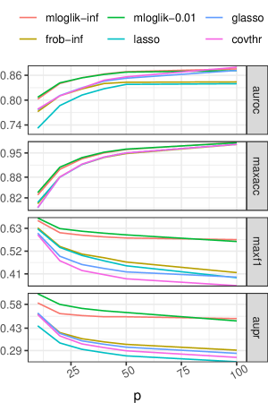
Figure 2: Structure recovery simulation results. Average evaluation metrics (rows) as a function of the model size for different algorithms (colors).

Data was standardized, which means that all methods used the empirical correlation matrix, $\hat{R}$, of the sample, and for lasso we fixed $C$ to the identity matrix. Finally, Algorithm 1 was initialized with the stable and symmetric matrix $B_{0}=-\frac{1}{2}\hat{R}^{-1}$ fulfilling $\hat{R}=\Sigma(B_{0},I_{p})$.

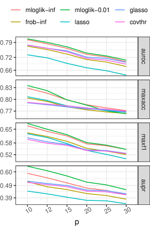
Figure 3: Recovery of marginalized model simulation results. Average evaluation metrics (rows) as a function of the model size for different algorithms (colors).

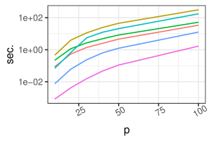
Figure 4: Average run times as a function of the system size ($p$) for different methods (colors).

4.2 RESULTS

Each method gives a solution path of graphs for a sequence of regularization parameters. We computed the following metrics to evaluate the methods:

• The path-wise maximum accuracy of edge recovery (maxacc).

• The path-wise maximum F1 score (maxf1).

• The area under the ROC curves (auroc), obtained as the true positive rate vs the false positive rate for each value of the regularization parameter.

• The area under the precision-recall curves (aupr), obtained as the precision vs the recall for each value of the regularization parameter.

All the above metrics were computed considering the graph recovery as a classification problem over the $p(p-1)$ off-diagonal elements of the adjacency matrix. In particular, undirected graphs obtained with the methods glasso and covthr are evaluated as directed graphs where each undirected edge is translated into the two possible directed edges.

Figure 2 shows the results from the simulation experiments averaged over the $100$ repetitions and the different edge densities, Figure 3 shows the results from the simulation experiment with marginalized models.

From Figure 2 we observe that among our proposed methods, using the negative log-likelihood was always better than the Frobenius loss. Across all simulations, mloglik-inf and mloglik-0.01 were clearly superiors to the other methods with respect to all our evaluation metrics. For these two methods the evaluations were highly similar with the exception of the precision-recall curve where mloglik-0.01 obtained consistently higher results, especially in the recovery of marginalized models. Moreover, we observe that frob-inf was superior to lasso in the recovery of the true graph with respect to almost all the metrics.

In Figure 4 the average run times of the different methods are reported. We observe that there is practically no difference in the run times between fixing $C=I_{p}$ (mloglik-inf) and allowing the estimation of a diagonal $C$ matrix (mloglik-0.01). Also it is interesting to note that the run time of the lasso method is equal to the mloglik methods for large systems. While frob-inf requires approximately one order of magnitude more time to reach convergence (or the maximum number of iterations) then mloglik-inf. Given that each iteration of Algorithm 1 is computationally more expensive using the negative log-likelihood than the Frobenius loss, we deduce that frob-inf requires in general a much higher number of iterations to converge.

5 PROTEIN-SIGNALING NETWORKS

We apply the proposed method with log-likelihood loss to the flow-cytometry data in Sachs et al. (2005) containing observations of $11$ phosphorylated proteins and phospholipids from $n=7466$ cells. Data were recorded under nine different conditions consisting of nine different stimulatory and inhibitory interventions.

We apply the following procedure, inspired by stability selection methods (Meinshausen and Bühlmann, 2010).

1. Randomly split the observations in two subsets with the same cardinality: Train and Test.

2. Apply Algorithm 1 using the estimated correlation matrix from Test, to obtain the estimated $B$ matrices along a regularization path.

3. Fit the maximum-likelihood estimators (using a minor modification of Algorithm 1 with $\lambda=0$) for all the structures obtained in the previous point.

4. Select the structure that obtains the maximum likelihood with respect to the empirical covariance matrix of Test.

After repeating $200$ times the above selection based on random-splitting we compute the number of times each edge was selected.

Figure 5 shows the resulting graph obtained by retaining directed edges appearing in at least $85\%$ of the repetitions.

We observe that the method retrieves edges consistent with the ground truth of conventionally accepted interactions (Sachs et al., 2005; Meinshausen et al., 2016). In particular, the estimated graph in Figure 5 contains 8 of the 18 edges reported in Sachs et al. (2005), among them: the regulatory interactions between PKA and Mek, p38, Erk; the relationships JNK $\leftarrow$ PKC $\rightarrow$ p38; and PLC $\rightarrow$ PIP2 $\leftarrow$ PIP3. We observe that our model estimate also some cycles, in particular the interactions PLC $\leftrightarrow$ PIP2, JNK $\leftrightarrow$ PKC $\leftrightarrow$ P38 and Mek $\leftrightarrow$ Raf which have been recovered in the literature by other approaches (Meinshausen et al., 2016).

Figure 5: Estimated graph from data in Sachs et al. (2005). Self loops and bidirected edges are not plotted.

6 DISCUSSION

We have presented a novel graphical model yielding a parametrization of covariance matrices via solutions of the continuous Lyapunov equation with parameter matrices $(B,C)$ compatible with a given mixed graph. Using a trek representation and a graphical projection we showed that also marginalized models can be parametrized by the continuous Lyapunov equation.

We investigated the performance of learning the directed part of the graph via penalized loss minimization where we fixed $C$ to be a diagonal matrix. A similar approach was considered by Fitch (2019) where, moreover, the matrix $C$ was fixed as the identity $I_{p}$. As shown in Section 2.3, marginalization may result in the $C$ matrix being increasingly misspecified and non-diagonal, thus the general deterioration of the performances for mloglik-inf, mloglik-0.01, frob-inf and lasso as in our simulation experiment is to be expected.

It was pivotal for our implementation of the proximal gradient algorithm that gradients for the loss functions could be computed as efficiently as possible. This was achieved via the representation of the Jacobian of $\Sigma(B,I)$ via Lyapunov equations and exploiting the adjoint of the linear operator $\Sigma(B,\cdot)$. When compared to the direct lasso path as proposed by Fitch (2019), our methods are computationally comparable, and even faster for larger systems, it appears. Moreover, our simulation experiment showed that minimizing the $\ell_{1}$-penalized negative log-likelihood resulted in a more efficient estimator of the directed part of the graph than using the Frobenius loss.

6.1 FUTURE DIRECTIONS

One open problem is to estimate $C$ as a non-diagonal, but sparse, matrix corresponding to the bidirected edges of the graph. This is particularly interesting when we consider data from a marginalized model. Imposing an additional penalty of the type $\lambda\rho_{1}(C)$ the corresponding proximal gradient-step is easily implemented to jointly estimate sparse matrices $(B,C)$. However, the optimization problem becomes highly non-convex, and initial experiments suggest that the algorithm is easily trapped in local minima. We conjecture that these computational problems are closely related to the fundamental open problem of determining the joint identifiability of the $B$ and $C$ parameters from $\Sigma$. It is ongoing work to provide answers to such identifiability questions and to devise algorithms that are able to jointly estimate $B$ and $C$.

6.2 REPRODUCIBILITY

Instructions and source files to replicate the examples and the experiments can be found at https://github.com/gherardovarando/gclm_experiments. An R package is available from https://github.com/gherardovarando/gclm, implementing Algorithm 1.

Acknowledgements

The authors thank Mathias Drton for insightful discussions and feedback. This work was supported by VILLUM FONDEN (grant 13358).

References

- Anderson et al. (1999) E. Anderson, Z. Bai, C. Bischof, S. Blackford, J. Demmel, J. Dongarra, J. Du Croz, A. Greenbaum, S. Hammarling, A. McKenney, and D. Sorensen. LAPACK Users’ Guide. Society for Industrial and Applied Mathematics, Philadelphia, PA, third edition, 1999.
- Bartels and Stewart (1972) R. H. Bartels and G. W. Stewart. Solution of the matrix equation AX + XB = C. Commun. ACM, 15(9):820–826, 1972.
- Basso et al. (2005) K. Basso, A. A. Margolin, G. Stolovitzky, U. Klein, R. Dalla-Favera, and A. Califano. Reverse engineering of regulatory networks in human B cells. Nature Genetics, 37:382 – 390, 2005.
- Beck and Tabulle (2010) A. Beck and M. Tabulle. Gradient-based algorithms with applications to signal recovery problems. In D. Palomar and Y. Eldar, editors, Convex Optimization in Signal Processing and Communications, pages 42–88. Cambridge University Press, 2010.
- Bhatia (1997) R. Bhatia. A note on the Lyapunov equation. Linear Algebra and its Applications, 259:71 – 76, 1997.
- Drton (2018) M. Drton. Algebraic problems in structural equation modeling. In The 50th Anniversary of Gröbner Bases, pages 35–86, Tokyo, Japan, 2018. Mathematical Society of Japan.
- Efron et al. (2004) B. Efron, T. Hastie, I. Johnstone, and R. Tibshirani. Least angle regression. Ann. Statist., 32(2):407–499, 04 2004.
- Fitch (2019) K. Fitch. Learning directed graphical models from Gaussian data. arXiv:1906.08050, 2019.
- Foygel et al. (2012) R. Foygel, J. Draisma, and M. Drton. Half-trek criterion for generic identifiability of linear structural equation models. Ann. Statist., 40(3):1682–1713, 06 2012.
- Friedman et al. (2007) J. Friedman, T. Hastie, and R. Tibshirani. Sparse inverse covariance estimation with the graphical lasso. Biostatistics, 9(3):432–441, 12 2007.
- Friedman et al. (2010) J. Friedman, T. Hastie, and R. Tibshirani. Regularization paths for generalized linear models via coordinate descent. Journal of Statistical Software, 33(1):1–22, 2010.
- Friedman et al. (2018) J. Friedman, T. Hastie, and R. Tibshirani. glasso: Graphical Lasso: Estimation of Gaussian Graphical Models, 2018. R package version 1.10.
- Horn and Johnson (1991) R. A. Horn and C. R. Johnson. Topics in Matrix Analysis. Cambridge University Press, 1991.
- Hyttinen et al. (2012) A. Hyttinen, F. Eberhardt, and P. O. Hoyer. Learning linear cyclic causal models with latent variables. Journal of Machine Learning Research, 13:3387–3439, 2012.
- Jacobsen (1991) M. Jacobsen. A brief account of the theory of homogeneous Gaussian diffusions in finite dimension. In Niemi, H. et.al, editor, Frontiers in Pure and Applied Probability, volume 1, pages 86–94, 1991.
- Malagò et al. (2018) L. Malagò, L. Montrucchio, and G. Pistone. Wasserstein Riemannian geometry of Gaussian densities. Information Geometry, 1(2):137–179, 2018.
- Meinshausen and Bühlmann (2010) N. Meinshausen and P. Bühlmann. Stability selection. Journal of the Royal Statistical Society: Series B (Statistical Methodology), 72(4):417–473, 2010.
- Meinshausen et al. (2016) N. Meinshausen, A. Hauser, J. M. Mooij, J. Peters, P. Versteeg, and P. Bühlmann. Methods for causal inference from gene perturbation experiments and validation. Proceedings of the National Academy of Sciences, 113(27):7361–7368, 2016.
- Mogensen and Hansen (2020) S. W. Mogensen and N. R. Hansen. Markov equivalence of marginalized local independence graphs. Ann. Statist., 48(1):539–559, 2020.
- Mogensen et al. (2018) S. W. Mogensen, D. Malinsky, and N. R. Hansen. Causal learning for partially observed stochastic dynamical systems. In Proceedings of the UAI, 2018.
- Parikh and Boyd (2014) N. Parikh and S. Boyd. Proximal algorithms. Found. Trends Optim., 1(3):127–239, 2014.
- Richardson and Spirtes (2002) T. Richardson and P. Spirtes. Ancestral graph Markov models. Ann. Statist., 30(4):962–1030, 08 2002.
- Sachs et al. (2005) K. Sachs, O. Perez, D. Pe’er, D. A. Lauffenburger, and G. P. Nolan. Causal protein-signaling networks derived from multiparameter single-cell data. Science, 308(5721):523–529, 2005.
- Sojoudi (2016) S. Sojoudi. Equivalence of graphical lasso and thresholding for sparse graphs. Journal of Machine Learning Research, 17(115):1–21, 2016.
- Sokol and Hansen (2014) A. Sokol and N. R. Hansen. Causal interpretation of stochastic differential equations. Electron. J. Probab., 19(100):1–24, 2014.
- Sullivant et al. (2010) S. Sullivant, K. Talaska, and J. Draisma. Trek separation for Gaussian graphical models. Ann. Statist., 38(3):1665–1685, 06 2010.
- Wright (1921) S. Wright. Correlation and causation. Journal of Agricultural Research, 20(7):557–585, 1921.
- Wright (1934) S. Wright. The method of path coefficients. Ann. Math. Statist., 5(3):161–215, 09 1934.
- Young et al. (2019) W. C. Young, K. Y. Yeung, and A. E. Raftery. Identifying dynamical time series model parameters from equilibrium samples, with application to gene regulatory networks. Statistical Modelling, 19(4):444–465, 2019.