Transfer Learning via Contextual Invariants for One-to-Many Cross-Domain Recommendation

Abstract.

The rapid proliferation of new users and items on the social web has aggravated the gray-sheep user/long-tail item challenge in recommender systems. Historically, cross-domain co-clustering methods have successfully leveraged shared users and items across dense and sparse domains to improve inference quality. However, they rely on shared rating data and cannot scale to multiple sparse target domains (i.e., the one-to-many transfer setting). This, combined with the increasing adoption of neural recommender architectures, motivates us to develop scalable neural layer-transfer approaches for cross-domain learning. Our key intuition is to guide neural collaborative filtering with domain-invariant components shared across the dense and sparse domains, improving the user and item representations learned in the sparse domains. We leverage contextual invariances across domains to develop these shared modules, and demonstrate that with user-item interaction context, we can learn-to-learn informative representation spaces even with sparse interaction data. We show the effectiveness and scalability of our approach on two public datasets and a massive transaction dataset from Visa, a global payments technology company (19% Item Recall, 3x faster vs. training separate models for each domain). Our approach is applicable to both implicit and explicit feedback settings.

1. Introduction

The focus of this paper is to learn to build expressive neural collaborative representations of users and items with sparse interaction data. The problem is essential: neural recommender systems are crucial to suggest useful products, services, and content to users online. Sparsity, or the long tail of user interaction, remains a central challenge to traditional collaborative filtering, as well as new neural collaborative filtering (NCF) approaches (He et al., 2017b). Sparsity challenges have become pronounced in neural models (Krishnan et al., 2018) owing to generalization and overfitting challenges, motivating us to learn-to-learn effective embedding spaces in such a scenario. Cross-domain transfer learning is a well-studied paradigm to address sparsity in recommendation. However, how recommendation domains are defined plays a key role in deciding the algorithmic challenges. In the most common pairwise cross-domain setting, we can employ cross-domain co-clustering via shared users or items (Wang et al., 2019; Man et al., 2017), latent structure alignment (Gao et al., 2013), or hybrid approaches using both (Hu et al., 2019; Perera and Zimmermann, 2019). However, recommendation domains with limited user-item overlap are pervasive in real-world applications, such as geographic regions with disparities in data quality and volume (e.g., restaurant recommendation in cities vs. sparse towns). Historically, there is limited work towards such a few-dense-source, multiple-sparse-target setting, where entity overlap approaches are ineffective. Further, sharing user data entails privacy concerns (Gao et al., 2019).

Simultaneously, context-aware recommendation has become an effective alternative to traditional methods owing to the extensive multi-modal feedback from online users (Mei et al., 2018). Combinations of contextual predicates prove critical in learning-to-organize the user and item latent spaces in recommendation settings. For instance, an Italian wine restaurant is a good recommendation for a high spending user on a weekend evening. However, it is a poor choice for a Monday afternoon, when the user is at work. The intersection of restaurant type (an attribute), historical patterns (historical context), and interaction time (interaction context) jointly describe the likelihood of this interaction. Our key intuition is to infer such behavioral invariants from a dense-source domain where we have ample interaction histories of users with wine restaurants and apply (or adapt) these learned invariants to improve inference in sparse-target domains. Clustering users who interact under covariant combinations of contextual predicates in different domains lets us better incorporate their behavioral similarities, and analogously, for the item sets as well. The user and item representations in sparse domains can be significantly improved when we combine these transferrable covariances.

Guiding neural representations is also a central theme in gradient-based meta-learning. Recent work (Finn et al., 2017; Li et al., 2017) measures the plasticity of a base-learner via gradient feedback for few-shot adaptation to multiple semantically similar tasks. However, the base-learner is often constrained to simpler architectures (such as shallow neural networks) to prevent overfitting (Sun et al., 2018) and requires multi-task gradient feedback at training time (Finn et al., 2017). This strategy does not scale to the embedding learning problem in NCF, especially in the many sparse-target setting.

Instead, we propose to incorporate the core strengths of meta-learning and transfer learning by defining transferrable neural layers (or meta-layers) via contextual predicates, working in tandem with and guiding domain-specific representations. Further, we develop a novel adaptation approach via regularized residual learning to incorporate new target domains with minimal overheads. Only residual layers and user/item embeddings are learned in each domain while transferring meta-layers, thus also limiting sparse domain overfit. In summary, we make the following contributions:

Contextual invariants for disjoint domains::

We identify the shared task of learning-to-learn NCF embeddings via cross-domain contextual invariances. We develop a novel class of pooled contextual predicates to learn descriptive representations in sparse recommendation domains without sharing users or items.

Tackling the one-dense, many-sparse scenario::

Our model infers invariant contextual associations via user-item interactions in the dense source domain. Unlike gradient-based meta-learning, we do not sample all domains at train time. We show that it suffices to transfer the source layers to new target domains with an inexpensive and effective residual adaptation strategy.

Modular Architecture for Reuse::

Contextual invariants describing user-item interactions are geographically and temporally invariant. Thus we can reuse our meta-layers while only updating the user and item spaces with new data, unlike black-box gradient strategies (Finn et al., 2017). This also lets us embed new users and items without retraining the model from scratch.

Strong Experimental Results::

We demonstrate strong experimental results with transfer between dense and sparse recommendation domains in three different datasets - (Yelp Challenge Dataset, Google Local Reviews) for benchmarking purposes and a large financial transaction dataset from Visa, a major global payments technology company. We demonstrate performance and scalability gains on multiple sparse target regions with low interaction volumes and densities by leveraging a single dense source region.

We now summarize related work, formalize our problem, describe our approach, and evaluate the proposed framework.

2. Related Work

We briefly summarize a few related lines of work that apply to the sparse inference problem in recommendation:

Sparsity-Aware Cross-Domain Transfer: Structure transfer methods regularize the user and item subspaces via principal components (Li et al., 2009; Pan et al., 2010), joint factorization (Jiang et al., 2017; Liu et al., 2013), shared and domain-specific cluster structure (Gao et al., 2013; Perera and Zimmermann, 2019) or combining prediction tasks (Sankar et al., 2020; Krishnan et al., 2019) to map user-item preference manifolds. They explicitly map correlated cluster structures in the subspaces. Instead, co-clustering methods use user or item overlaps as anchors for sparse domain inference (Man et al., 2017; Wang et al., 2019), or auxiliary data (Volkovs et al., 2017; Jiang et al., 2014) or both (Hu et al., 2019). It is hard to quantify the volume of users/items or shared content for effective transfer. Further, both overlap-based methods and pairwise structure transfer do not scale to many sparse-targets.

Neural Layer Adaptation: A wide-array of layer-transfer and adaptation techniques use convolutional invariants on semantically related images (Long et al., 2017; Sun and Saenko, 2016) and graphs (Sankar et al., 2019). However, unlike convolutional nets, latent collaborative representations are neither interpretable nor permutation invariant (He et al., 2017b; Liang et al., 2018). Thus it is much harder to establish principled layer-transfer methods for recommendation. We develop our model architecture via novel contextual invariants to enable cross-domain layer-transfer and adaptation.

Meta-Learning in Recommendation: Prior work has considered algorithm selection (Chen et al., 2018), hyper-parameter initialization (Feurer et al., 2015; Du et al., 2019), shared scoring functions across users (Vartak et al., 2017) and meta-curriculums to train models on related tasks (Du et al., 2019; Lee et al., 2019). Across these threads, the primary challenge is scalability in the multi-domain setting. Although generalizable, they train separate models (over users in  (Vartak et al., 2017)), which can be avoided by adapting or sharing relevant components.

3. Problem Definition

Consider recommendation domains $\mathbb{D}=\{\mathbf{D}_{i}\}$ where each $\mathbf{D}_{i}$ is a tuple $\{\mathcal{U}_{\mathbf{D}_{i}},\mathcal{V}_{\mathbf{D}_{i}},\mathcal{T}_{\mathbf{D}_{i}}\}$, with $\mathcal{U}_{\mathbf{D}_{i}}$, $\mathcal{V}_{\mathbf{D}_{i}}$ denoting the user and item sets of $\mathbf{D}_{i}$, and interactions $\mathcal{T}_{\mathbf{D}_{i}}$ between them. There is no overlap between the user and item sets of any two domains $\mathbf{D}_{i}$, $\mathbf{D}_{j}$.

In the implicit feedback setting, each interaction $t\in\mathcal{T}_{\mathbf{D}_{i}}$ is a tuple $t=(u,\mathbf{c},v)$ where $u\in\mathcal{U}_{\mathbf{D}_{i}},v\in\mathcal{V}_{\mathbf{D}_{i}}$ and context vector $\mathbf{c}\in\mathbb{R}^{|\mathbf{C}|}$. For the explicit feedback setting, $\mathcal{T}_{\mathbf{D}_{i}}$ is replaced by ratings $\mathcal{R}_{\mathbf{D}_{i}}$, where each rating is a tuple $r=(u,\mathbf{c},v,r_{uv})$, with the rating value $r_{uv}$ (other notations are the same). For simplicity, all interactions in all domains have the same set of context features. In our datasets, the context feature set $\mathbf{C}$ contains three different types of context features, interactional features $\mathbf{C}_{\mathbf{I}}$ (such as time of interaction), historical features $\mathbf{C}_{\mathbf{H}}$ (such as a user’s average spend), and attributional features $\mathbf{C}_{\mathbf{A}}$ (such as restaurant cuisine or user age). Thus each context vector $\mathbf{c}$ contains these three types of features for that interaction, i.e., $\mathbf{c}=[\mathbf{c}_{\mathbf{I}},\mathbf{c}_{\mathbf{H}},\mathbf{c}_{\mathbf{A}}]$.

Under implicit feedback, we rank items $v\in\mathcal{V}_{\mathbf{D}}$ given user $u\in\mathcal{U}_{\mathbf{D}}$ and context $\mathbf{c}$. In the explicit feedback scenario, we predict rating $r_{uv}$ for $v\in\mathcal{V}_{\mathbf{D}}$ given $u\in\mathcal{U}_{\mathbf{D}}$ and $\mathbf{c}$. Our transfer objective is to reduce the rating or ranking error in a set of disjoint sparse target domains $\{\mathbf{D}_{t}\}\subset\mathbb{D}$ given the dense source domain $\mathbf{D}_{s}\in\mathbb{D}$.

4. Our Approach

In this section, we describe a scalable, modular architecture to extract pooled contextual invariants and employ them to guide the learned user and item embedding spaces.

4.1. Modular Architecture

We achieve context-guided embedding learning via four synchronized neural modules with complementary semantic objectives:

• Context Module $\mathcal{M}^{1}$: Extracts contextual invariants driving user-item interactions in the dense source domain.

• Embedding Modules $\mathcal{M}^{2}_{\mathcal{U}},\mathcal{M}^{2}_{\mathcal{V}}$: Domain-specific user and item embedding spaces ($\mathcal{U}$, $\mathcal{V}$ denote users and items).

• Context-conditioned Clustering Modules $\mathcal{M}^{3}_{\mathcal{U}},\mathcal{M}^{3}_{\mathcal{V}}$:
  $\mathcal{M}^{3}_{\mathcal{U}}$ and $\mathcal{M}^{3}_{\mathcal{V}}$ reorient the user and item embeddings with the contextual invariants extracted by $\mathcal{M}^{1}$ respectively.

• Mapping/Ranking Module $\mathcal{M}^{4}$: Generate interaction likelihoods with the context-conditioned representations of $\mathcal{M}^{3}$.

Context-driven modules $\mathcal{M}^{1}$, $\mathcal{M}^{3}$, and $\mathcal{M}^{4}$ contain the meta-layers that are transferred from the dense to the sparse domains (i.e., shared or meta-modules), while $\mathcal{M}^{2}$ contains the domain-specific user and item representations. Our architecture provides a separation between the domain-specific $\mathcal{M}^{2}$ module and shared context-based transforms in the other modules (Figure 1).

4.2. Module Description

We now detail each module in our overall architecture.

4.2.1. Context Module $\mathcal{M}^{1}$

User-item interactions are driven by context feature intersections that are inherently multiplicative (i.e., assumptions of independent feature contributions are insufficient), and are often missed in the Naive-Bayes assumption of additive models such as feature attention (He and Chua, 2017; Beutel et al., 2018). Inspired by the past success of low-rank feature pooling (Kim et al., 2016; Beutel et al., 2018), our context module extracts low-rank multi-linear combinations of context to describe interactions and build expressive representations. The first layer in $\mathcal{M}^{1}$ transforms context $\mathbf{c}$ of an interaction $(u,\mathbf{c},v)$ as follows:

(1) $$\mathbf{c}^{2}=\sigma(\underbrace{\mathbf{W}^{2}\mathbf{c}\oplus(\mathbf{b}^{2}\otimes\mathbf{c})}_{\text{Weighted linear transform}})\hskip 10.0pt\otimes\underbrace{\mathbf{c}}_{\text{Element-wise interaction}}$$

where $\oplus,\otimes$ denote element-wise product and sum, i.e.,

(2) $$\mathbf{c}^{2}_{i}\propto\mathbf{c}_{i}\times\sigma(\mathbf{b}^{2}_{i}\mathbf{c}_{i}+\sum_{j}\mathbf{W}^{2}_{ij}\mathbf{c}_{j})\vspace{-8pt}$$

Thus, $\mathbf{c}^{2}_{i}$ ($i^{th}\text{-component}$ of $\mathbf{c}^{2}$) incorporates a weighted bivariate interaction between $\mathbf{c}_{i}$ and other context factors $\mathbf{c}_{j}$, including itself. We then repeat this transformation over multiple stacked layers with each layer using the previous output:

(3) $$\mathbf{c}^{n}=\sigma(\mathbf{W}^{n}\mathbf{c}^{n-1}\oplus(\mathbf{b}^{n}\otimes\mathbf{c}^{n-1}))\otimes\mathbf{c}$$

Each layer interacts n-variate terms from the previous layer with $\mathbf{c}$ to form n+1-variate terms. However, since each layer has only $|\mathbf{C}|$ outputs (i.e., low-rank), $\mathbf{W}^{n}$ prioritizes the most effective n-variate combinations of $\mathbf{c}$ (typically, a very small fraction of all combinations is useful). We can choose the number of layers $n_{\mathbf{C}}$ depending on the required order of the final combinations $\mathbf{c}^{n_{\mathcal{C}}}$.

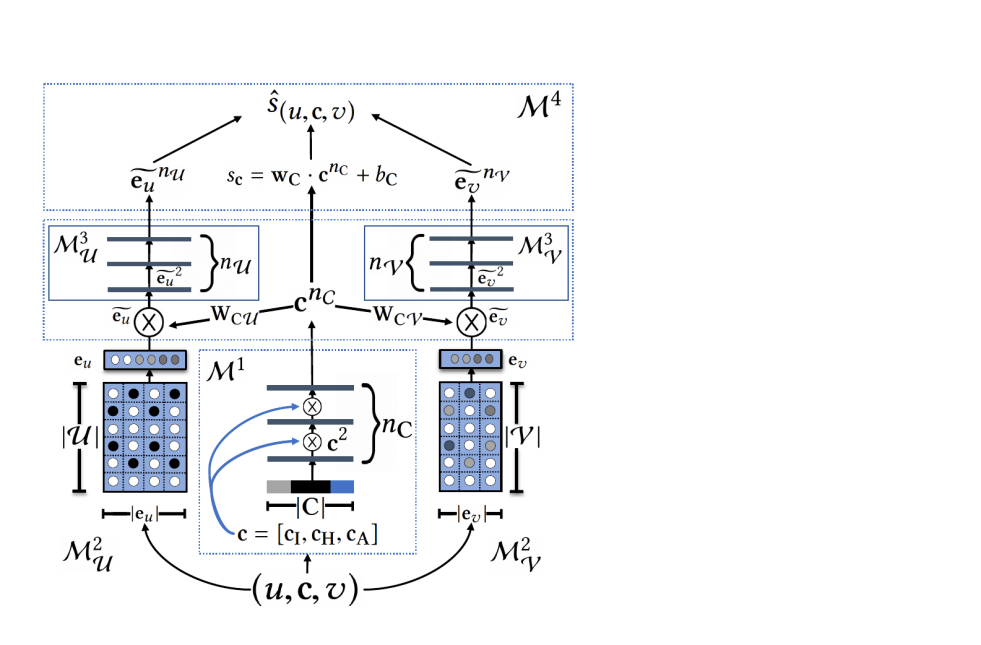
Figure 1. Our overall recommender architecture, highlighting all four modules, $\mathcal{M}^{1}\text{ to }\mathcal{M}^{4}$

Multimodal Residuals for Discriminative Correlation Mining: In addition to discovering the most important context combinations, we incorporate the information gain associated with pairwise interactions of context features (Tang et al., 2014). For instance, the item cost feature is more informative in interactions where users deviate from their historical spending patterns. Specifically, pairs of signals (e.g., cost & user history) enhance or diminish each other’s impact, i.e.,

(4) $$\mathbf{c}_{i}=\mathbf{c}_{i}+\Sigma_{j}\delta_{\mathbf{c}_{i}|\mathbf{c}_{j}}$$

We simplify Equation 4 by only considering cross-modal effects across interactional, historical and attributional context, i.e.,

(5) $$\delta_{\mathbf{c}_{\mathbf{I}}|\mathbf{c}_{\mathbf{H}},\mathbf{c}_{\mathbf{A}}}=\underbrace{\mathbf{s_{\mathbf{I}}}}_{\text{Scaling factor}}\otimes\hskip 7.0pt\underbrace{\textit{tanh}(\mathbf{W}_{\mathbf{IH}}\times\mathbf{c}_{\mathbf{H}}+\mathbf{W}_{\mathbf{IA}}\times\mathbf{c}_{\mathbf{A}}+\mathbf{b}_{\mathbf{I}})}_{\text{Info gain/loss}}$$

and likewise for $\delta_{\mathbf{c}_{\mathbf{H}}}$, $\delta_{\mathbf{c}_{\mathbf{A}}}$. Information gains are computed before $\mathbf{c}^{2}$ to cascade to further layers.

Table 1. Modules and Learned Parameter Notations

Modules	Learned Parameters
Domain-Specific	Embeddings $\mathbf{e}_{u}\forall u\in\mathcal{U}_{\mathbf{D}}$, $\mathbf{e}_{v}\forall v\in\mathcal{V}_{\mathbf{D}}$
($\mathcal{M}^{2}_{\mathcal{U}},\mathcal{M}^{2}_{\mathcal{V}}$)	Biases (only under explicit feedback) $s,s_{u}\forall u\in\mathcal{U}_{\mathbf{D}},s_{v}\forall v\in\mathcal{V}_{\mathbf{D}}$
Shared Modules	$\mathcal{M}^{1}$   eq. 3   $(\mathbf{W}^{i},\mathbf{b}^{i})\forall i=[1,\cdots,n_{\mathbf{C}}]$
	$\mathcal{M}^{1}$   eq. 5   $\mathbf{s}_{\mathbf{I}},\mathbf{s}_{\mathbf{H}},\mathbf{s}_{\mathbf{A}};\mathbf{W}_{\mathbf{I}},\mathbf{W}_{\mathbf{H}},\mathbf{W}_{\mathbf{A}}$
($\mathcal{M}^{1}$, $\mathcal{M}^{3},\mathcal{M}^{4}$)	$\mathcal{M}^{3}$   eq. 7   $\mathbf{W}_{\mathbf{C}\mathcal{U}},\mathbf{W}_{\mathbf{C}\mathcal{V}}$
	$\mathcal{M}^{3}_{\mathcal{U}}$ eq. 9   $(\mathbf{W}^{i}_{\mathcal{U}},\mathbf{b}^{i}_{\mathcal{U}})\forall i=[1,\cdots,n_{\mathcal{U}}]$
	$\mathcal{M}^{3}_{\mathcal{V}}$ eq. 9   $(\mathbf{W}^{i}_{\mathcal{V}},\mathbf{b}^{i}_{\mathcal{V}})\forall i=[1,\cdots,n_{\mathcal{V}}]$
	$\mathcal{M}^{4}$   eq. 10   $\mathbf{W}_{\mathbf{C}},\mathbf{b}_{\mathbf{C}}$

4.2.2. Context Conditioned Clustering $\mathcal{M}^{3}$

We combine domain-specific embeddings $\mathcal{M}^{2}$ with the context combinations extracted by $\mathcal{M}^{1}$ to generate context-conditioned user and item representations. Specifically, we introduce the following bilinear transforms,

(6) $$\widetilde{\mathbf{e}_{u}}=\mathbf{e}_{u}\otimes\sigma(\mathbf{W}_{\mathbf{C}\mathcal{U}}\times\mathbf{c}^{n_{\mathbf{C}}})$$

(7) $$\widetilde{\mathbf{e}_{v}}=\mathbf{e}_{v}\otimes\sigma(\mathbf{W}_{\mathbf{C}\mathcal{V}}\times\mathbf{c}^{n_{\mathbf{C}}})$$

where, $\mathbf{W}_{\mathbf{C}\mathcal{U}}\in\mathbb{R}^{{|\mathbf{e}_{u}|\times|\mathbf{C}}|}$, $\mathbf{W}_{\mathbf{C}\mathcal{V}}\in\mathbb{R}^{{|\mathbf{e}_{v}|\times|\mathbf{C}}|}$ are learned parameters that map the most relevant context combinations to the user and item embeddings. We further introduce $n_{\mathcal{U}}$ feedforward RelU layers to cluster the representations,

(8) $$\widetilde{\mathbf{e}_{u}}^{2}=\sigma(\mathbf{W}_{\mathcal{U}}^{2}\widetilde{\mathbf{e}_{u}}+\mathbf{b}_{\mathcal{U}}^{2})$$

(9) $$\widetilde{\mathbf{e}_{u}}^{n}=\sigma(\mathbf{W}_{\mathcal{U}}^{n}\widetilde{\mathbf{e}_{u}}^{n-1}+\mathbf{b}_{\mathcal{U}}^{n})$$

Analogously, we obtain context-conditioned item representations $\widetilde{\mathbf{e}_{v}}^{2},\cdots,\widetilde{\mathbf{e}_{v}}^{n_{\mathcal{V}}}$ with $n_{\mathcal{V}}$ feedforward RelU layers.

The bilinear transforms in eq. 7 introduce dimension alignment for both $\widetilde{\mathbf{e}_{u}}^{n_{\mathcal{U}}}$ and $\widetilde{\mathbf{e}_{v}}^{n_{\mathcal{V}}}$ with the context output $\mathbf{c}^{n_{\mathbf{C}}}$. Thus, when $\mathcal{M}^{3}$ and $\mathcal{M}^{1}$ layers are transferred to a sparse target domain, we can directly backpropagate to guide the target domain user and item embeddings with the target domain interactions.

4.3. Source Domain Training Algorithm

In the source domain, we train all modules and parameters (Table 1) with ADAM optimization (Kingma and Ba, 2014) and dropout regularization (Srivastava et al., 2014).

4.3.1. Self-paced Curriculum via Contextual Novelty

Focusing on harder data samples accelerates and stabilizes stochastic gradients (Loshchilov and Hutter, 2015; Chang et al., 2017). Since our learning process is grounded on context, novel interactions display uncommon or interesting context combinations. Let $\mathcal{L}_{(u,\mathbf{c},v)}$ denote the loss function for an interaction $(u,\mathbf{c},v)$. We propose an inverse novelty measure referred as the context-bias, $s_{\mathbf{c}}$, which is self-paced by the context combinations learned by $\mathcal{M}^{1}$ in Equation 3,

(10) $$s_{\mathbf{c}}=\mathbf{w}_{\mathbf{C}}\cdot\mathbf{c}^{n_{\mathbf{C}}}+b_{\mathbf{C}}$$

We then attenuate the loss $\mathcal{L}_{(u,\mathbf{c},v)}$ for this interaction as,

(11) $$\mathcal{L}_{(u,\mathbf{c},v)}^{\mathbf{{}^{\prime}}}=\mathcal{L}_{(u,\mathbf{c},v)}-s_{\mathbf{c}}$$

The resulting novelty loss $\mathcal{L}_{(u,\mathbf{c},v)}^{\mathbf{{}^{\prime}}}$ decorrelates interactions (Cogswell et al., 2015; Johnson and Zhang, 2013) by emulating variance-reduction in the n-variate pooled space of $\mathbf{c}^{n_{\mathbf{C}}}$. $\mathcal{L}_{(u,\mathbf{c},v)}^{\mathbf{{}^{\prime}}}$ determines the user and item embedding spaces, inducing a novelty-weighted training curriculum focused on harder samples as training proceeds. We now describe loss $\mathcal{L}_{(u,\mathbf{c},v)}$ for the explicit and implicit feedback scenarios.

4.3.2. Ranking our Recommendations

In the implicit feedback setting, predicted likelihood $\hat{s}_{(u,\mathbf{c},v)}$ is computed with the context-conditioned embeddings (Equation 9) and context-bias (Equation 11) as,

(12) $$\hat{s}_{(u,\mathbf{c},v)}=\widetilde{\mathbf{e}_{u}}^{n_{\mathcal{U}}}\cdot\widetilde{\mathbf{e}_{v}}^{n_{\mathcal{V}}}+s_{\mathbf{c}}$$

The loss for all the possible user-item-context combinations in domain $\mathbf{D}$ is,

(13) $$\mathcal{L}_{\mathbf{D}}=\sum_{u\in\mathcal{U}_{\mathbf{D}}}\sum_{v\in\mathcal{V}_{\mathbf{D}}}\sum_{\mathbf{c}\in\mathbb{R}^{|\mathbf{c}|}}||\mathbb{I}_{(u,\mathbf{c},v)}-\hat{s}_{(u,\mathbf{c},v)}||^{2}$$

where $\mathbb{I}$ is the binary indicator $(u,\mathbf{c},v)\in\mathcal{T}_{\mathbf{D}}$. $\mathcal{L}_{\mathbf{D}}$ is intractable due to the large number of contexts $\mathbf{c}\in\mathbb{R}^{|\mathbf{c}|}$. We develop a negative sampling approximation for implicit feedback with two learning objectives - identify the likely item given the user and interaction context, and identify the likely context given the user and the item. We thus construct two negative samples for each $(u,\mathbf{c},v)\in\mathcal{T}_{\mathbf{D}}$ at random: Item negative with the true context, $(u,\mathbf{c},v^{-})$ and context negative with the true item, $(u,\mathbf{c}^{-},v)$. $\mathcal{L}_{\mathbf{D}}$ then simplifies to,

(14) $$\mathcal{L}_{\mathbf{D}}=\sum_{\mathcal{T}_{\mathbf{D}}}||1-\hat{s}_{(u,\mathbf{c},v)}||^{2}+\sum_{(u,\mathbf{c},v^{-})}||\hat{s}_{(u,\mathbf{c},v^{-})}||+\sum_{(u,\mathbf{c}^{-},v)}||\hat{s}_{(u,\mathbf{c}^{-},v)}||$$

In the explcit feedback setting, we introduce two additional bias terms, one for each user, $s_{u}$ and one for each item, $s_{v}$. These terms account for user and item rating eccentricities (e.g., users who always rate well), so that the embeddings are updated with the relative rating differences. Finally, global bias $s$ accounts for the rating scale, e.g., 0-5 vs. 0-10. Thus the predicted rating is given as,

(15) $$\hat{r}_{(u,\mathbf{c},v)}=\widetilde{\mathbf{e}_{v}}^{n_{\mathcal{V}}}\cdot\widetilde{\mathbf{e}_{u}}^{n_{\mathcal{U}}}+s_{\mathbf{c}}+s_{u}+s_{v}+s$$

Negative samples are not required in the explicit feedback setting,

(16) $$\mathcal{L}_{\mathbf{D}}^{explicit}=\sum_{(u,\mathbf{c},v,r_{uv})\in\mathcal{R}_{\mathbf{D}}}||r_{uv}-\hat{r}_{(u,\mathbf{c},v)}||^{2}$$

We now detail our approach to transfer the shared modules from the source domain to sparse target domains.

5. Transfer to Target Domains

Our formulation enables us to train the shared modules $(\mathcal{M}^{1})_{\mathbf{S}},(\mathcal{M}^{3})_{\mathbf{S}}$ and $(\mathcal{M}^{4})_{\mathbf{S}}$ on a dense source domain $\mathbf{S}$, and transfer them to a sparse target domain $\mathbf{T}$ to guide its embedding module $(\mathcal{M}^{2})_{\mathbf{T}}$. Each shared module $\mathcal{M}$ encodes inputs $\mathbf{x}_{\mathcal{M}}$ to generate output representations $\mathbf{y}_{\mathcal{M}}$. In each domain $\mathbf{T}$, module $(\mathcal{M})_{\mathbf{T}}$ determines the joint input-output distribution,

(17) $$p_{\mathbf{T}}(\mathbf{y}_{\mathcal{M}},\mathbf{x}_{\mathcal{M}})=p_{\mathbf{T}}(\mathbf{y}_{\mathcal{M}}|\mathbf{x}_{\mathcal{M}})\times p_{\mathbf{T}}(\mathbf{x}_{\mathcal{M}})$$

where the parameters of $(\mathcal{M})_{\mathbf{T}}$ determine the conditional $p_{\mathbf{T}}(\mathbf{y}_{\mathcal{M}}|\mathbf{x}_{\mathcal{M}})$ and $p_{\mathbf{T}}(\mathbf{x}_{\mathcal{M}})$ describes the inputs to module $(\mathcal{M})_{\mathbf{T}}$ in domain ${\mathbf{T}}$. Adaptation: There are two broad strategies to adapt module $\mathcal{M}$ to a new target domain ${\mathbf{T}}$:

• Parameter Adaptation: We can retrain the parameters of module $\mathcal{M}$ for target domain $\mathbf{T}$ thus effectively changing the conditional $p_{\mathbf{T}}(\mathbf{y}_{\mathcal{M}}|\mathbf{x}_{\mathcal{M}})$ in eq. 17, or,

• Input Adaptation: Modify the input distribution $p_{\mathbf{T}}(\mathbf{x}_{\mathcal{M}})$ in each domain $\mathbf{T}$ without altering the parameters of $\mathcal{M}$.

We now explore module transfer with both types of adaptation strategies towards achieving three key objectives. First, the transferred modules must be optimized to be effective on each target domain $\mathbf{T}$. Second, we aim to minimize the computational costs of adapting to new domains by maximizing the reuse of module parameters between the source $\mathbf{S}$ and target domains $\mathbf{T}$. Finally, we must take care to avoid overfitting the transferred modules to the samples in the sparse target domain $\mathbf{T}$.

5.1. Direct Layer-Transfer

We first train all four modules on the source $\mathbf{S}$ and each target domain $\mathbf{T}$ in isolation. We denote these pre-trained modules as $(\mathcal{M}^{i})_{\mathbf{S}}$ and $(\mathcal{M}^{i})_{\mathbf{T}}$ for source domain $\mathbf{S}$ and a target domains $\mathbf{T}$ respectively. We then replace the shared modules in all the target domain models with the source-trained version, i.e., $(\mathcal{M}^{1})_{\mathbf{T}}=(\mathcal{M}^{1})_{\mathbf{S}}$, $(\mathcal{M}^{3})_{\mathbf{T}}=(\mathcal{M}^{3})_{\mathbf{S}}$, $(\mathcal{M}^{4})_{\mathbf{T}}=(\mathcal{M}^{4})_{\mathbf{S}}$, while the domain-specific embeddings $(\mathcal{M}^{2})_{\mathbf{T}}$ are not changed in the target domains. Clearly, direct layer-transfer involves no overhead and trivially prevents overfitting. However, we need to adapt the transferred modules for optimal target performance, i.e., either adapt the parameters or the input distributions for the transferred modules in each target $\mathbf{T}$. We now develop these adaptation strategies building on layer-transfer.

Table 2. Comparing the objectives in Section 5 addressed by our meta-transfer approaches for sparse target domains

Adaptation Method	Target Adaptation	Resists Overfitting	Extra compute per target	Extra parameters per target
Layer-Transfer	No adaptation	Yes, trivially	None	None, module params reused
Simulated Annealing	Yes, module params	Yes, stochastic	All parameter updates	All module params ( Table 1)
Regularized Residuals	Yes, module inputs	Yes, via distributional consistency	Residual layer updates with distributional regularization	Residual layer parameters

5.2. Simulated Annealing

Simulated annealing is a stochastic local-search algorithm, that implicitly thresholds parameter variations in the gradient space by decaying the gradient learning rates (Kirkpatrick et al., 1983). As a simple and effective adaptation strategy, we anneal each transferred module $\mathcal{M}$ in the target domain $\mathbf{T}$ with exponentially decaying learning rates to stochastically prevent overfitting:

(18) $$(m)_{b+1}=(m)_{b}+\eta_{b}\frac{\partial\mathcal{L}_{b}}{\partial m},\hskip 3.0pt\eta_{b}=\eta_{0}e^{-\lambda b}$$

where $m$ denotes any parameter of transferred module $\mathcal{M}$ (Table 1), $b$ is the stochastic gradient batch index in the target domain and $\mathcal{L}_{b}$ is the batch loss for batch $b$. Our annealing strategy stochastically generates a robust parameter search schedule for transferred modules $\mathcal{M}^{1},\mathcal{M}^{3},\mathcal{M}^{4}$, with $\eta_{b}$ decaying to zero after one annealing epoch. While annealing the transferred modules, domain-specific module $\mathcal{M}^{2}$ is updated with the full learning rate $\eta_{0}$. Clearly, annealing modifies the conditional $p_{\mathbf{T}}(\mathbf{y}_{\mathcal{M}}|\mathbf{x}_{\mathcal{M}})$ in eq. 17 via parameter adaptation. However, annealing transferred modules in each target domain is somewhat expensive, and the annealed parameters are not shareable, thus causing scalability limitations in the one-to-many transfer scenario. We now develop a lightweight residual adaptation strategy to achieve input adaptation without modifying any shared module parameters in the target domains to overcome the above scalability challenges.

5.3. Distributionally Regularized Residuals

We now develop an approach to reuse the source modules with target-specific input adaptation, thus addressing the scalability concerns of parameter adaptation methods.

5.3.1. Enabling Module Reuse with Residual Input Adaptation

In eq. 17, module $\mathcal{M}$ implements the conditional $p(\mathbf{y}_{\mathcal{M}}|\mathbf{x}_{\mathcal{M}})$. To maximize parameter reuse, we share these modules across the source and target domains (i.e., $p_{\mathbf{T}}(\mathbf{y}_{\mathcal{M}}|\mathbf{x}_{\mathcal{M}})=p_{\mathbf{S}}(\mathbf{y}_{\mathcal{M}}|\mathbf{x}_{\mathcal{M}})$) and introduce target-specific residual perturbations to account for their eccentricities (Long et al., 2016) by modifying the input distributions $p_{\mathbf{T}}(\mathbf{x}_{\mathcal{M}})$. Target-specific input adaptation overcomes the need for an expensive end-to-end parameter search. Our adaptation problem thus reduces to learning an input modifier for each target domain $\mathbf{T}$ and shared module $\mathcal{M}\in[\mathcal{M}^{1},\mathcal{M}^{3},\mathcal{M}^{4}]$, i.e., for each $\mathcal{M},\mathbf{T}$. Residual transformations enable the flow of information between layers without the gradient attenuation of inserting new non-linear layers, resulting in numerous optimization advantages (He et al., 2016). Given the module-input $\mathbf{x}_{\mathcal{M}}$ to the shared module $\mathcal{M}$ in target domain $\mathbf{T}$, we learn a module and target specific residual transform:

(19) $$\mathbf{x}_{\mathcal{M}}=\mathbf{x}_{\mathcal{M}}+\delta_{\mathcal{M},\mathbf{T}}(\mathbf{x}_{\mathcal{M}})$$

The form of the residual function $\delta$ is flexible. We chose a single non-linear residual layer, $\delta(\mathbf{x})=tanh(\mathbf{W}\mathbf{x}+\mathbf{b})$. We can intuitively balance the complexity and number of such residual layers. Note that the above residual strategy involves learning the $\delta_{\mathcal{M},\mathbf{T}}$ layers with feedback from only the sparse target domain samples. To avoid overfitting, we need a scalable regularization strategy to regularize $p_{\mathbf{T}}(\mathbf{x}_{M})$ in each target domain. We propose to leverage the source input distribution as a common baseline for all the target domains, i.e., intuitively, $p_{\mathbf{S}}(\mathbf{x}_{M})$ provides a common center for each $p_{\mathbf{T}}(\mathbf{x}_{M})$ in the different target domains. This effectively anchors the residual functions and prevents overfitting to noisy samples.

5.3.2. Scalable Distributional Regularization for Residual Learning

Learning pairwise regularizers between each $p_{\mathbf{T}}(\mathbf{x}_{M})$ and the source input distribution $p_{\mathbf{S}}(\mathbf{x}_{M})$ is not a scalable solution. Instead we train a universal regularizer for each module $\mathcal{M}$ on the source $p_{\mathbf{S}}(\mathbf{x}_{\mathcal{M}})$, and apply this pre-trained regularizer when we fit the residual layers $\delta_{\mathcal{M},\mathbf{T}}$ in each target domain. Our key intuition is to treat the regularizer for the inputs of each module $\mathcal{M}$ as a one-class decision-boundary (Sabokrou et al., 2018), described by the dense regions in the source domain, i.e., $p_{\mathbf{S}}(\mathbf{x}_{\mathcal{M}})$. Unlike adversarial models that are trained with both the source and target distributions (Radford et al., 2015), we propose a novel approach to learn distributional input regularizers for the shared modules with just the source domain inputs. For each shared module, the learned regularizer anticipates hard inputs across the target domains without accessing the actual samples. We introduce a variational encoder $\mathcal{E}_{\mathcal{M}}$ with RelU layers to map inputs $\mathbf{x}_{\mathcal{M}}\sim p_{\mathbf{S}}(\mathbf{x}_{\mathcal{M}})$ to a lower-dimensional reference distribution $\mathbf{N}(0,\mathbb{I})$ (Doersch, 2016). Simultaneously, we add poisoning model $\mathcal{P}_{\mathcal{M}}$ to generate sample-adaptive noise $\mathcal{P}_{\mathcal{M}}(\mathbf{x}_{\mathcal{M}})$ to generate poisoned samples $\widetilde{\mathbf{x}}_{\mathcal{M}}=\mathbf{x}_{\mathcal{M}}+\mathcal{P}_{\mathcal{M}}(\mathbf{x}_{\mathcal{M}})$ with the source domain inputs $\mathbf{x}_{\mathcal{M}}\sim p_{\mathbf{S}}(\mathbf{x}_{\mathcal{M}})$. We define the encoder loss to train $\mathcal{E}_{\mathcal{M}}$ as follows:

(20) $$\mathcal{L}_{\mathcal{E}_{\mathcal{M}}}=D(p(\mathcal{E}_{\mathcal{M}}(\mathbf{x}_{\mathcal{M}}))\;\|\;\mathbf{N}(0,\mathbb{I}))-D(p(\mathcal{E}_{\mathcal{M}}(\widetilde{\mathbf{x}}_{\mathcal{M}}))\;\|\;\mathbf{N}(0,\mathbb{I}))$$

where $D(p\;\|\;q)$ denotes the KL-Divergence of distributions $p$ and $q$. The above loss enables $\mathcal{E}_{\mathcal{M}}$ to separate the true and poisoned samples across the $\mathbf{N}(0,\mathbb{I})$ hypersphere in its encoded space. Since $\mathcal{E}_{\mathcal{M}}(\mathbf{x}_{\mathcal{M}})$ involves a stochastic sampling step, gradients can be estimated with a reparametrization trick using random samples to eliminate stochasticity in the loss $\mathcal{L}_{\mathcal{E}_{\mathcal{M}}}$(Doersch, 2016). Conversely, the loss for our poisoning model $\mathcal{P}_{\mathcal{M}}$ is given by,

(21) $$\mathcal{L}_{\mathcal{P}_{\mathcal{M}}}=D(p(\mathcal{E}_{\mathcal{M}}(\widetilde{\mathbf{x}_{\mathcal{M}}}\;\|\;\mathbf{N}(0,\mathbb{I}))-\log||\mathcal{P}_{\mathcal{M}}(\mathbf{x}_{\mathcal{M}})||$$

Note the first term in Equation 21 attempts to confuse $\mathcal{E}_{\mathcal{M}}$ into encoding poisoned examples $\widetilde{\mathbf{x}_{\mathcal{M}}}=\mathbf{x}_{\mathcal{M}}+\mathcal{P}_{\mathcal{M}}(\mathbf{x}_{\mathcal{M}})$ in the reference distribution, while the second term prevents the degenerate solution $\mathcal{P}_{\mathcal{M}}(\mathbf{x}_{\mathcal{M}})=0$. Equation 20 and Equation 21 are alternatingly optimized, learning sharper decision boundaries as training proceeds. With the above alternating optimization, we pre-train the encoders $\mathcal{E}_{\mathcal{M}}$ for the three shared modules on the source domain $\mathbf{S}$. We now describe how we use these encoders to regularize the residual layers $\delta_{\mathcal{M},\mathbf{T}}$ in each target domain $\mathbf{T}$.

5.3.3. Distributionally-Regularized Target Loss

For each target domain $\mathbf{T}$, we learn three residual layers for the module inputs $\mathbf{c}^{2}$, $\widetilde{\mathbf{e}_{u}}$ and $\widetilde{\mathbf{e}_{v}}$ for $\mathcal{M}_{1},\mathcal{M}_{3}^{\mathcal{U}},\mathcal{M}_{3}^{\mathcal{V}}$ respectively. The inputs to $\mathcal{M}_{4}$, $\widetilde{\mathbf{e}_{u}}^{n_{\mathcal{U}}}$, $\widetilde{\mathbf{e}_{v}}^{n_{\mathcal{V}}}$ are not adapted. Thus, we learn three variational encoders in the source domain as described in Section 5.3.2, $\mathcal{E}_{\mathbf{C}},\mathcal{E}_{\mathcal{U}}$ and $\mathcal{E}_{\mathcal{V}}$ for $\mathbf{c}^{2}$, $\widetilde{\mathbf{e}_{u}}$ and $\widetilde{\mathbf{e}_{v}}$ respectively. Consider target interactions $(u,\mathbf{c},v)\in\mathcal{T}_{\mathbf{T}}$. In the absence of distributional regularization, the loss is identical to the first term in Equation 14. However, we now apply regularizers to $\mathbf{c}^{2}$, $\widetilde{\mathbf{e}_{u}},\widetilde{\mathbf{e}_{v}}$:

(22) $$\begin{split}\mathcal{L}^{reg}_{\mathcal{T}_{\mathbf{T}}}&=\mathcal{L}_{\mathcal{T}_{\mathbf{T}}}+D(p_{\mathbf{T}}(\mathcal{E}_{\mathcal{U}}({\widetilde{\mathbf{e}_{u}}}))\;\|\;\mathbf{N}(0,\mathbb{I}))+\\ &D(p_{\mathbf{T}}(\mathcal{E}_{\mathcal{V}}({\widetilde{\mathbf{e}_{v}}}))\;\|\;\mathbf{N}(0,\mathbb{I}))+D(p_{\mathbf{T}}(\mathcal{E}_{\mathbf{C}}({\mathbf{c}^{2}}))\;\|\;\mathbf{N}(0,\mathbb{I}))\end{split}$$

Again, the gradients can be estimated with the reparametrization trick on the stochastic KL-divergence terms(Doersch, 2016) as in Section 5.3.2. The residual layers are then updated as in Section 4.3 with $\mathcal{L}^{reg}_{\mathcal{T}_{\mathbf{T}}}$ replacing the first term in Equation 14.

6. Experimental Results

In this section, we present experimental analyses on diverse multi-domain recommendation datasets and show two key results. First, when we adapt modules trained on a rich source domain to the sparse target domains, we significantly reduce the computational costs and improve performance in comparison to learning directly on the sparse domains. Second, our model is comparable to state-of-the-art baselines when trained on a single domain without transfer.

Dataset		State	Users	Items	Interactions
	S	Bay-Area CA	1.20 m	8.90 k	25.0 m
FT-Data	$\mathbf{T}_{1}$	Arkansas	0.40 m	3.10 k	5.20 m
$|\mathbf{C}|=220$	$\mathbf{T}_{2}$	Kansas	0.35 m	2.90 k	5.10 m
	$\mathbf{T}_{3}$	New-Mexico	0.32 m	2.80 k	6.20 m
	$\mathbf{T}_{4}$	Iowa	0.30 m	3.00 k	4.80 m
	S	Pennsylvania	10.3 k	5.5 k	170 k
Yelp	$\mathbf{T}_{1}$	Alberta, Canada	5.10 k	3.5 k	55.0 k
$|\mathbf{C}|=120$	$\mathbf{T}_{2}$	Illinois	1.80 k	1.05 k	23.0 k
	$\mathbf{T}_{3}$	S.Carolina	0.60 k	0.40 k	6.20 k
Google	S	California	46 k	28 k	320 k
Local	$\mathbf{T}_{1}$	Colorado	10 k	5.7 k	51.0 k
$|\mathbf{C}|=90$	$\mathbf{T}_{2}$	Michigan	7.0 k	4.0 k	29.0 k
	$\mathbf{T}_{3}$	Ohio	5.4 k	3.2 k	23.0 k

Table 3. Source and Target statistics for each of our datasets. Source states denoted S have more interactions and interaction density per user than target states denoted $\mathbf{T}_{i}$.

6.1. Datasets and Baselines

We evaluate our recommendation model both with and without module transfer over the publicly available Yelp and Google Local Reviews datasets for benchmarking purposes. Reviews are split across U.S and Canadian states in these datasets. We treat each state as a separate recommendation domain for training and transfer purposes. There is no user or item overlap across the states (recommendation domains) in any of our datasets. We repeat our experiments with a large-scale restaurant transaction dataset obtained from Visa (referred to as FT-Data), also split across U.S. states.

Google Local Reviews Dataset (Explicit feedback)(He et al., 2017a; Pasricha and McAuley, 2018)::

Users rate businesses on a 0-5 scale with temporal, spatial, and textual context available for each review. We also infer additional context features - users’ preferred locations on weekdays and weekends, spatial patterns and preferred product categories.

Yelp Challenge Dataset (Explicit feedback) ::

Users rate restaurants on a 0-5 scale, reviews include similar context features as the Google Local dataset. Further, user check-ins and restaurant attributes (e.g., accepts-cards) are available.

FT-Data (Implicit feedback)::

Contains the credit/debit card payments of users to restaurants in the U.S, with spatial, temporal, financial context features, and inferred transaction attributes. We leverage transaction histories also to infer user spending habits, restaurant popularity, peak hours, and tipping patterns.

In each dataset, we extract the same context features for every state with state-wise normalization, either with min-max normalization or quantile binning. We retain users and items with three or more reviews in the Google Local dataset and ten or more reviews in the Yelp dataset. In FT-Data, we retain users and restaurants with over ten, twenty transactions, respectively, over three months. In each dataset, we choose a dense state with ample data as the source domain where all modules are trained, and multiple sparse states as target domains for module transfer from the source.

6.1.1. Source to Target Module Transfer

We evaluate the performance gains obtained when we transfer or adapt modules $\mathcal{M}^{1},\mathcal{M}^{3}$ and $\mathcal{M}^{4}$ from the source state to each target state, in comparison to training all four modules directly on the target. We also compare target domain gains with state-of-the-art meta-learning baselines:

:

LWA (Vartak et al., 2017): Learns a shared meta-model across all domains, with a user-specific linear component.

:

NLBA (Vartak et al., 2017): Replaces LWA’s linear component with a neural network with user-specific layer biases.

:

$\mathbf{s^{2}}$-Meta (Du et al., 2019): Develops a meta-learner to instantiate and train recommender models for each scenario. In our datasets, scenarios are the different states.

Direct Layer-Transfer (Our Variant)::

Transfers source-trained meta-modules to the target-trained models as in Section 5.1.

Anneal (Our Variant)::

We apply simulated annealing to adapt the transferred meta-modules to the target as in Section 5.2.

DRR - Distributionally Regularized Residuals: :

(Our Main Approach) Adapts the inputs of each transferred module with separate residual layers in each target state. (Section 5.3).

6.1.2. Single Domain Recommendation Performance

We also evaluate the performance of our models independently without transfer on the source and target states in each dataset. We compare with the following state-of-the-art recommendation baselines:

:

NCF (He et al., 2017b): State-of-the-art non context-aware model for comparisons and context validation.

:

CAMF-C (Baltrunas et al., 2011): Augments Matrix Factorization to incorporate a context-bias term for item latent factors. This version assumes a fixed bias for a given context feature for all items.

:

CAMF (Baltrunas et al., 2011): CAMF-C with separate context bias values for each item. We use this version for comparisons.

:

MTF (Karatzoglou et al., 2010): Obtains latent representations via decomposition of the User-Item-Context tensor. This model scales very poorly with the size of the context vector.

:

NFM (He and Chua, 2017): Employs a bilinear interaction model applied to the context features of each interaction for representation.

:

AFM (Xiao et al., 2017): Incorporates an attention mechanism to reweight the bilinear pooled factors in the NFM model. Scales poorly with the number of pooled contextual factors.

:

AIN (Mei et al., 2018): Reweights the interactions of user and item representations with each contextual factor via attention.

:

MMT-Net (Our Main Approach): We refer to our model with all four modules as Multi-Linear Module Transfer Network (MMT-Net).

:

FMT-Net (Our Variant): We replace $\mathcal{M}^{1}$s layers with feedforward RelU layers to demonstrate the importance of multiplicative context invariants.

:

MMT-Net Multimodal (Our Variant): MMT-Net with the information-gain terms described in Equation 5. Only applied to FT-Data due to lack of interactional features in other datasets.

6.1.3. Experiment Setup

We tune each baseline in parameter ranges centered at the author provided values for each dataset and set all embedding dimensions to $200$ for uniformity. We split each state in each dataset into training (80%), validation (10%), and test (10%) sets for training, tuning, and testing purposes. For the implicit feedback setting in FT-Data, we adopt the standard negative-sample evaluation (He et al., 2017b) and draw one-hundred negatives per positive, equally split between item and context negatives similar to the training process in Section 4.3. We then evaluate the average Hit-Rate@K (H@K) metric for $K=1,5$ in Table 8, indicating if the positive sample was ranked highly among the negative samples. For the explicit feedback setting in the other two datasets, we follow the standard RMSE and MAE metrics in Table 7 (Baltrunas et al., 2011; Mei et al., 2018) (no negative samples required). All models were implemented with Tensorflow and tested on a Nvidia Tesla V100 GPU.

Table 4. Comparing aspects addressed by baseline recommendation models against our proposed MMT-Net approach

	Bi-Linear Pooling	Multi-Linear Pooling	Low-Rank	Factor Weights	$\mathbf{\Theta}$(Context)
NFM	Yes	No	No	No	Linear
AFM	Yes	No	No	Yes	Quadratic
AIN	No	No	Yes	Yes	Linear
FMT	No	No	Yes	Yes	Linear
MMT	Yes	Yes	Yes	Yes	Linear

6.2. Module Transfer to Sparse Target States

Dataset		Direct	Anneal	DRR	LWA	NLBA	$\mathbf{s^{2}}$-Meta
		%H@1	%H@1	%H@1	%H@1	%H@1	%H@1
FT-Data	$T_{1}$	2%	19%	18%	6%	x	x
	$T_{2}$	0%	16%	16%	8%	x	x
	$T_{3}$	3%	18%	18%	6%	x	x
	$T_{4}$	-1%	14%	12%	11%	x	x

Table 5. Percentage improvements (% Hit-Rate@1) on FT-Data target states with module transfer approaches and meta-learning baselines against training all modules on the target state directly as in Table 8.

We evaluate module transfer methods by the percentage improvements in the Hit-Rate@1 for the implicit feedback setting in FT-Data (Table 5), or the drop in RMSE (Table 6) for the explicit feedback datasets when we transfer the $\mathcal{M}^{1},\mathcal{M}^{3}$ and $\mathcal{M}^{4}$ modules from the source state rather than training all four modules from scratch on that target domain. Similarly, meta-learning baselines were evaluated by comparing their joint meta-model performance on the target state against our model trained only on that state. The performance numbers for training our model on each target state without transfer are recorded in Table 7, Table 8. We could not scale the NLBA, LWA and $\mathbf{s^{2}}$-Meta approaches to FT-Data owing to the costs of training the meta-models on all users combined across the source and multiple target domains. In Table 6, we demonstrate the percentage reduction in RMSE with module transfer for Google Local, Yelp, and in Table 5, we demonstrate significant improvements in the hit-rates for FT-Data. We start with an analysis of the training process for module transfer with simulated annealing and DRR adaptation.

Table 6. Percentage RMSE improvements on the Yelp and Google Local target states with module transfer approaches and meta-learning baselines against training all modules on the target state directly as in Table 7.

Dataset		Direct	Anneal	DRR	LWA	NLBA	$\mathbf{s^{2}}$-Meta
		%RMSE	%RMSE	%RMSE	%RMSE	%RMSE	%RMSE
Yelp	$T_{1}$	-2.2%	7.7%	7.2%	2.6%	4.1%	3.7%
	$T_{2}$	-2.6%	9.0%	7.9%	1.8%	3.6%	3.1%
	$T_{3}$	0.8%	8.5%	8.1%	0.3%	5.3%	1.8%
Google	$T_{1}$	-1.2%	11.2%	11.0%	3.3%	4.3%	3.1%
Local	$T_{2}$	-1.7%	12.1%	10.9%	4.6%	4.9%	2.8%
	$T_{3}$	-2.0%	9.6%	8.8%	2.4%	6.3%	3.9%

Transfer Details: On each target state in each dataset, all four modules of our MMT-Net model are pretrained over two gradient epochs on the target samples. The layers in modules $\mathcal{M}^{1},\mathcal{M}^{3}$ and $\mathcal{M}^{4}$ are then replaced with those trained on the source state, while retaining module $\mathcal{M}^{2}$ without any changes (in our experiments $\mathcal{M}^{2}$ just contains user and item embeddings, but could also include neural layers if required). This is then followed by either simulated annealing or DRR adaptation of the transferred modules. We analyze the training loss curves in Section 6.4.2 to better understand the fast adaptation of the transferred modules.

Invariant Quality: A surprising result was the similar performance of direct layer-transfer with no adaptation to training all modules on the target state from scratch (Table 6). The transferred source state modules were directly applicable to the target state embeddings. This helps us validate the generalizability of context-based modules across independently trained state models even with no user or item overlap.

Computational Gains: We also plot the total training times including pretraining for DRR and annealing against the total number of target state interactions in Figure 5. On the target states, module transfer is  3x faster then training all the modules from scratch. On the whole, there is a significant reduction in the overall training time and computational effort in the one-to-many setting. Simulated annealing and DRR adaptation converge in fewer epochs when applied to the pre-trained target model, and outperform the target-trained model by significant margins (Table 6). These computational gains potentially enable a finer target domain granularity (e.g., adapt to towns or counties rather than states).

Table 7. We evaluate recommendation performance on each state (no transfer) with RMSE, MAE metrics for explicit feedback against the ground-truth ratings. Metrics were averaged over five runs, $*$ indicates statistical significance (paired t-test, p=0.05). On average, models incorporating both pooling and reweighting in Table 4 exhibit significant relative gains (i.e., AFM, MMT).

Dataset	State	CAMF (Baltrunas et al., 2011)		MTF (Karatzoglou et al., 2010)		NCF (He et al., 2017b)		NFM (He and Chua, 2017)		AFM (Xiao et al., 2017)		AIN (Mei et al., 2018)		FMT-Net		MMT-Net
		RMS	MAE	RMS	MAE	RMS	MAE	RMS	MAE	RMS	MAE	RMS	MAE	RMS	MAE	RMS	MAE
Yelp	S	1.21	0.94	1.13	0.87	1.18	1.04	1.02	0.83	0.96	0.78	0.98	0.75	1.02	0.76	0.94	0.73
	$T_{1}$	1.56	1.20	1.41	1.12	1.39	0.99	1.29	1.01	1.27	0.94	1.36	0.91	1.34	0.95	1.24*	0.88*
	$T_{2}$	1.33	1.04	1.36	0.98	1.26	1.02	1.19	1.05	1.16	0.90	1.17	0.95	1.15	0.98	1.13*	0.91
	$T_{3}$	1.49	1.13	1.50	1.08	1.35	1.08	1.31	0.96	1.20*	0.93	1.25	0.98	1.29	1.02	1.20*	0.89*
	S	1.36	1.01	1.21	0.90	1.04	0.89	0.80	0.73	0.77	0.63	0.85	0.64	0.91	0.68	0.77	0.64
Google	$T_{1}$	1.49	1.20	1.38	1.14	1.27	1.05	1.10	0.99	0.94	0.85	1.22	0.90	1.31	0.96	0.89	0.76*
Local	$T_{2}$	1.37	1.16	1.31	1.20	1.36	1.17	1.21	1.05	1.14*	0.98	1.19	1.01	1.28	1.07	1.16	0.93*
	$T_{3}$	1.39	1.23	1.20	1.07	1.19	0.98	1.13	0.92	1.09	0.91	1.08	0.94	1.14	0.98	1.02*	0.85*

Dataset	State	CAMF	MTF	NCF (He et al., 2017b)		NFM (He and Chua, 2017)		AFM	AIN (Mei et al., 2018)		FMT-Net		MMT-Net		MMT-m
		(Baltrunas et al., 2011)	(Karatzoglou et al., 2010)	H@1	H@5	H@1	H@5	(Xiao et al., 2017)	H@1	H@5	H@1	H@5	H@1	H@5	H@1	H@5
FT-Data	S	x	x	0.42	0.77	0.52	0.91	x	0.44	0.89	0.37	0.76	0.56*	0.94	0.56*	0.93
	$T_{1}$	x	x	0.36	0.71	0.41	0.83	x	0.34	0.76	0.32	0.75	0.45	0.84	0.47*	0.86*
	$T_{2}$	x	x	0.25	0.64	0.30	0.77	x	0.30	0.72	0.26	0.72	0.34*	0.79	0.34*	0.77
	$T_{3}$	x	x	0.26	0.70	0.31	0.78	x	0.29	0.74	0.28	0.74	0.33	0.82*	0.34	0.80
	$T_{4}$	x	x	0.29	0.72	0.32	0.74	x	0.32	0.78	0.21	0.69	0.37	0.80	0.38	0.83*

Table 8. We evaluate recommendation performance on each state (no transfer) with the H@1, 5 metrics for implicit feedback in FT-Data. Metrics were averaged over five runs, * indicates statistical significance (paired t-test, p=0.05). On average, feature-pooling methods AFM, NFM and MMT outperform additive models AIN, FMT. x indicates timed-out or memory limit exceeded.

6.3. Single Domain Recommendation

6.3.1. Comparative Analysis

We draw attention to the most relevant features of the baselines and our variants in Table 4. We highlight our key observations from the experimental results obtained with the baseline recommenders and our FMT-Net and MMT-Net variants (Table 8, Table 7). Note that methods with some form of context pooling significantly outperform those without pooled factors, indicating the importance of multi-linear model expressivity to handle interaction context.

We note that AFM performs competitively owing to its ability to reweight terms, similar to our approach (Table 7), but fails to scale to the larger FT-Data. NFM is linear with context size owing to a simple algebraic re-organization, and thus scales to FT-Data, however losing the ability to reweight pairwise context product terms (He and Chua, 2017). Also note the differences between our FMT and MMT variants, demonstrating the importance of the pooled multi-linear formulation for the contextual invariants. These performance differences are more pronounced in the implicit feedback setting (Table 8). This can be attributed to the greater relevance of transaction context (e.g., transactions provide accurate temporal features while review time is a proxy to the actual visit) and more context features in FT-Data vs. Google Local and Yelp (220 vs. 90,120 respectively), magnifying the importance of feature pooling for FT-Data.

The lack of pooled feature expressivity in the FMT-Net model impacts the training process as seen in Figure 4, demonstrating the importance of context intersection. The NFM and MMT models converge faster to a smaller Train-RMSE in Figure 4 and outperform FMT on the test data (Table 8, Table 7). We also observe models incorporating pooled factors to outperform the inherently linear attention-based AIN model, although the performance gap is less pronounced in the smaller review datasets (Table 7). We now qualitatively analyze our results to interpret module adaptation.

6.4. Qualitative Analysis

We analyze our approach from the shared module training and convergence perspective for the different adaptation methods. We observe consistent trends across the direct layer-transfer, annealing, and DRR adaptation approaches.

6.4.1. Training without Context-Bias

To understand the importance of decorrelating training samples in the training process, we repeat the performance analysis on our MMT-Net model with and without the adaptive context-bias term in the training objective in Section 4.3. We observe a 15% performance drop across the Yelp and Google Local datasets, although this does not reflect in the Train-RMSE convergence (Figure 2) of the two variations. In the absence of context-bias, the model overfits uninformative transactions to the user and item bias terms ($s_{u}$, $s_{v}$) in Equation 15, Equation 16 and thus achieves comparable Train-RMSE values. However, the overfit user and item terms are not generalizable, resulting in the observed drop in test performance.

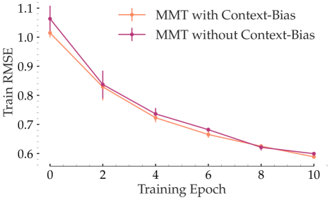
Figure 2. MMT-Net trained with & without context-bias (Equation 11) on the Google Local source exhibits similar Train-RMSE, but registers $>10\%$ drop in test performance.

6.4.2. Model Training and Convergence Analysis

We compare the Train-RMSE convergence for the MMT-Net model fitted from scratch to the Google Local target state, Colorado ($\mathbf{T}_{1}$) vs. the training curve under DRR and annealing adaptation with two pretraining epochs on the target state in Figure 3. Clearly, the target-trained model takes significantly longer to converge to a stable Train-RMSE in comparison to the Anneal and DRR adaptation. Although the final Train-RMSE is comparable (Figure 5), there is a significant performance difference between the two approaches on the test dataset, as observed in Table 6. Training loss convergence alone is not indicative of the final model performance; the target-only training method observes lower Train-RMSE by overfitting to the sparse data. We also compare the Train-RMSE convergence for target-trained models with and without pooled context factors (MMT-Net, NFM vs. FMT-Net) in Figure 4. We observe the NFM, MMT-Net models to converge faster to a better optimization minima than FMT-Net. This also reflects in their test performance in Table 8.

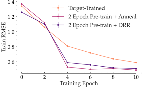
Figure 3. MMT-Net convergence under target-training vs. Annealing/DRR adaptation after 2 epochs of pretraining on the Google Local Colorado target

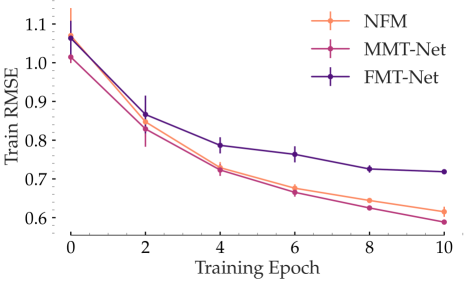
Figure 4. MMT-Net convergence compared to NFM and FMT-Net on the Google Local Colorado target

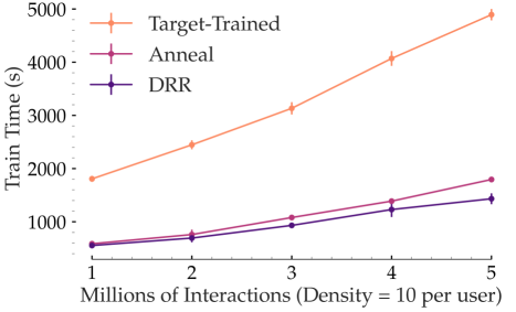
Figure 5. MMT-Net training duration with and without module transfer vs. target domain interaction volume

6.5. Scalability and Robustness Analysis

We demonstrate the scalability of meta-transfer with the number of transactions in the target domain in Figure 5 against training separate models. Our previous observations in Section 6.2 validate the ability of our approach to scale deeper architectures to a large number of target domains while also enabling a finer resolution for the selection of target domains. Towards tackling incomplete data, we also evaluated the robustness of the shared context layers by randomly dropping up to 20% of the context features in each interaction at train and test time for both, the source and target states in Table 9.

Table 9. MMT-Net performance degradation was measured by the decrease in H@1 or increase in RMSE, averaged over target states with random context feature dropout

Context Drop	5%	10%	15%	20%
FT-Data	1.1%	2.6%	4.1%	6.0%
Google Local	3.9%	4.2%	7.0%	8.8%
Yelp	1.8%	3.2%	5.4%	7.3%

6.6. Limitations and Discussion

We identify a few fundamental limitations of our model. While our approach presents a scalable and effective solution to bridge the weaknesses of gradient-based meta learning and co-clustering via user or item overlaps, contextual invariants do not extend to cold-start users or items. Second, our model does not trivially extend to the case where a significant number of users or items are shared across recommendation domains. We separate the embeddings and learn-to-learn aspect which improves modularity, but prevents direct reuse of representations across domains, since only the transformation layers are shared. Depending on the application, context features could potentially be filtered to enhance social inference and prevent loss of diversity in the generated recommendations.

7. Conclusion

This paper proposes a novel approach to address the sparsity problem in the cross-domain setting. We leverage the strengths of meta-transfer learning, grounded on an expressive context pooling strategy to learn effective invariants. Our approach is highly scalable in the one-to-many setting, incurs minimal costs to accommodate new sparse target domains, and significantly outperforms competing methods in our experimental results. A few interesting future directions include updating representation with streaming data and incorporating knowledge priors on expected behavior patterns (e.g., if we knew what combinations of context are more likely to dictate interactions) to benefit the learned context transformation space.

References

- (1)
- Baltrunas et al. (2011) Linas Baltrunas, Bernd Ludwig, and Francesco Ricci. 2011. Matrix factorization techniques for context aware recommendation. In Proceedings of the fifth ACM conference on Recommender systems. ACM, 301–304.
- Beutel et al. (2018) Alex Beutel, Paul Covington, Sagar Jain, Can Xu, Jia Li, Vince Gatto, and Ed H Chi. 2018. Latent cross: Making use of context in recurrent recommender systems. In Proceedings of the Eleventh ACM International Conference on Web Search and Data Mining. ACM, 46–54.
- Chang et al. (2017) Haw-Shiuan Chang, Erik Learned-Miller, and Andrew McCallum. 2017. Active bias: Training more accurate neural networks by emphasizing high variance samples. In Advances in Neural Information Processing Systems. 1002–1012.
- Chen et al. (2018) Fei Chen, Zhenhua Dong, Zhenguo Li, and Xiuqiang He. 2018. Federated meta-learning for recommendation. arXiv preprint arXiv:1802.07876 (2018).
- Cogswell et al. (2015) Michael Cogswell, Faruk Ahmed, Ross Girshick, Larry Zitnick, and Dhruv Batra. 2015. Reducing overfitting in deep networks by decorrelating representations. arXiv preprint arXiv:1511.06068 (2015).
- Doersch (2016) Carl Doersch. 2016. Tutorial on variational autoencoders. arXiv preprint arXiv:1606.05908 (2016).
- Du et al. (2019) Zhengxiao Du, Xiaowei Wang, Hongxia Yang, Jingren Zhou, and Jie Tang. 2019. Sequential Scenario-Specific Meta Learner for Online Recommendation. arXiv preprint arXiv:1906.00391 (2019).
- Feurer et al. (2015) Matthias Feurer, Jost Tobias Springenberg, and Frank Hutter. 2015. Initializing bayesian hyperparameter optimization via meta-learning. In Twenty-Ninth AAAI Conference on Artificial Intelligence.
- Finn et al. (2017) Chelsea Finn, Pieter Abbeel, and Sergey Levine. 2017. Model-agnostic meta-learning for fast adaptation of deep networks. In Proceedings of the 34th International Conference on Machine Learning-Volume 70. JMLR. org, 1126–1135.
- Gao et al. (2019) Chen Gao, Xiangning Chen, Fuli Feng, Kai Zhao, Xiangnan He, Yong Li, and Depeng Jin. 2019. Cross-domain Recommendation Without Sharing User-relevant Data. In The World Wide Web Conference. ACM, 491–502.
- Gao et al. (2013) Sheng Gao, Hao Luo, Da Chen, Shantao Li, Patrick Gallinari, and Jun Guo. 2013. Cross-domain recommendation via cluster-level latent factor model. In Joint European conference on machine learning and knowledge discovery in databases. Springer, 161–176.
- He et al. (2016) Kaiming He, Xiangyu Zhang, Shaoqing Ren, and Jian Sun. 2016. Deep residual learning for image recognition. In Proceedings of the IEEE conference on computer vision and pattern recognition. 770–778.
- He et al. (2017a) Ruining He, Wang-Cheng Kang, and Julian McAuley. 2017a. Translation-based recommendation. In Proceedings of the Eleventh ACM Conference on Recommender Systems. ACM, 161–169.
- He and Chua (2017) Xiangnan He and Tat-Seng Chua. 2017. Neural factorization machines for sparse predictive analytics. In Proceedings of the 40th International ACM SIGIR conference on Research and Development in Information Retrieval. ACM, 355–364.
- He et al. (2017b) Xiangnan He, Lizi Liao, Hanwang Zhang, Liqiang Nie, Xia Hu, and Tat-Seng Chua. 2017b. Neural collaborative filtering. In Proceedings of the 26th international conference on world wide web. International World Wide Web Conferences Steering Committee, 173–182.
- Hu et al. (2019) Guangneng Hu, Yu Zhang, and Qiang Yang. 2019. Transfer Meets Hybrid: A Synthetic Approach for Cross-Domain Collaborative Filtering with Text. In The World Wide Web Conference. ACM, 2822–2829.
- Jiang et al. (2014) Meng Jiang, Peng Cui, Fei Wang, Xinran Xu, Wenwu Zhu, and Shiqiang Yang. 2014. Fema: flexible evolutionary multi-faceted analysis for dynamic behavioral pattern discovery. In Proceedings of the 20th ACM SIGKDD international conference on Knowledge discovery and data mining. ACM, 1186–1195.
- Jiang et al. (2017) Shuhui Jiang, Zhengming Ding, and Yun Fu. 2017. Deep low-rank sparse collective factorization for cross-domain recommendation. In Proceedings of the 25th ACM international conference on Multimedia. ACM, 163–171.
- Johnson and Zhang (2013) Rie Johnson and Tong Zhang. 2013. Accelerating stochastic gradient descent using predictive variance reduction. In Advances in neural information processing systems. 315–323.
- Karatzoglou et al. (2010) Alexandros Karatzoglou, Xavier Amatriain, Linas Baltrunas, and Nuria Oliver. 2010. Multiverse recommendation: n-dimensional tensor factorization for context-aware collaborative filtering. In Proceedings of the fourth ACM conference on Recommender systems. ACM, 79–86.
- Kim et al. (2016) Jin-Hwa Kim, Kyoung-Woon On, Woosang Lim, Jeonghee Kim, Jung-Woo Ha, and Byoung-Tak Zhang. 2016. Hadamard product for low-rank bilinear pooling. arXiv preprint arXiv:1610.04325 (2016).
- Kingma and Ba (2014) Diederik P Kingma and Jimmy Ba. 2014. Adam: A method for stochastic optimization. arXiv preprint arXiv:1412.6980 (2014).
- Kirkpatrick et al. (1983) Scott Kirkpatrick, C Daniel Gelatt, and Mario P Vecchi. 1983. Optimization by simulated annealing. science 220, 4598 (1983), 671–680.
- Krishnan et al. (2019) Adit Krishnan, Hari Cheruvu, Cheng Tao, and Hari Sundaram. 2019. A modular adversarial approach to social recommendation. In Proceedings of the 28th ACM International Conference on Information and Knowledge Management. 1753–1762.
- Krishnan et al. (2018) Adit Krishnan, Ashish Sharma, Aravind Sankar, and Hari Sundaram. 2018. An Adversarial Approach to Improve Long-Tail Performance in Neural Collaborative Filtering. In Proceedings of the 27th ACM International Conference on Information and Knowledge Management. ACM, 1491–1494.
- Lee et al. (2019) Hoyeop Lee, Jinbae Im, Seongwon Jang, Hyunsouk Cho, and Sehee Chung. 2019. MeLU: Meta-Learned User Preference Estimator for Cold-Start Recommendation. In Proceedings of the 25th ACM SIGKDD International Conference on Knowledge Discovery & Data Mining. 1073–1082.
- Li et al. (2009) Bin Li, Qiang Yang, and Xiangyang Xue. 2009. Can movies and books collaborate? cross-domain collaborative filtering for sparsity reduction. In Twenty-First International Joint Conference on Artificial Intelligence.
- Li et al. (2017) Zhenguo Li, Fengwei Zhou, Fei Chen, and Hang Li. 2017. Meta-SGD: Learning to learn quickly for few-shot learning. arXiv preprint arXiv:1707.09835 (2017).
- Liang et al. (2018) Dawen Liang, Rahul G Krishnan, Matthew D Hoffman, and Tony Jebara. 2018. Variational autoencoders for collaborative filtering. In Proceedings of the 2018 World Wide Web Conference. International World Wide Web Conferences Steering Committee, 689–698.
- Liu et al. (2013) Jialu Liu, Chi Wang, Jing Gao, and Jiawei Han. 2013. Multi-view clustering via joint nonnegative matrix factorization. In Proceedings of the 2013 SIAM International Conference on Data Mining. SIAM, 252–260.
- Long et al. (2016) Mingsheng Long, Han Zhu, Jianmin Wang, and Michael I Jordan. 2016. Unsupervised domain adaptation with residual transfer networks. In Advances in Neural Information Processing Systems. 136–144.
- Long et al. (2017) Mingsheng Long, Han Zhu, Jianmin Wang, and Michael I Jordan. 2017. Deep transfer learning with joint adaptation networks. In Proceedings of the 34th International Conference on Machine Learning-Volume 70. JMLR. org, 2208–2217.
- Loshchilov and Hutter (2015) Ilya Loshchilov and Frank Hutter. 2015. Online batch selection for faster training of neural networks. arXiv preprint arXiv:1511.06343 (2015).
- Man et al. (2017) Tong Man, Huawei Shen, Xiaolong Jin, and Xueqi Cheng. 2017. Cross-Domain Recommendation: An Embedding and Mapping Approach.. In IJCAI. 2464–2470.
- Mei et al. (2018) Lei Mei, Pengjie Ren, Zhumin Chen, Liqiang Nie, Jun Ma, and Jian-Yun Nie. 2018. An attentive interaction network for context-aware recommendations. In Proceedings of the 27th ACM International Conference on Information and Knowledge Management. ACM, 157–166.
- Pan et al. (2010) Weike Pan, Evan Wei Xiang, Nathan Nan Liu, and Qiang Yang. 2010. Transfer learning in collaborative filtering for sparsity reduction. In Twenty-fourth AAAI conference on artificial intelligence.
- Pasricha and McAuley (2018) Rajiv Pasricha and Julian McAuley. 2018. Translation-based factorization machines for sequential recommendation. In Proceedings of the 12th ACM Conference on Recommender Systems. ACM, 63–71.
- Perera and Zimmermann (2019) Dilruk Perera and Roger Zimmermann. 2019. CnGAN: Generative Adversarial Networks for Cross-network user preference generation for non-overlapped users. In The World Wide Web Conference. ACM, 3144–3150.
- Radford et al. (2015) Alec Radford, Luke Metz, and Soumith Chintala. 2015. Unsupervised representation learning with deep convolutional generative adversarial networks. arXiv preprint arXiv:1511.06434 (2015).
- Sabokrou et al. (2018) Mohammad Sabokrou, Mohammad Khalooei, Mahmood Fathy, and Ehsan Adeli. 2018. Adversarially learned one-class classifier for novelty detection. In Proceedings of the IEEE Conference on Computer Vision and Pattern Recognition. 3379–3388.
- Sankar et al. (2019) Aravind Sankar, Xinyang Zhang, and Kevin Chen-Chuan Chang. 2019. Meta-GNN: metagraph neural network for semi-supervised learning in attributed heterogeneous information networks. In Proceedings of the 2019 IEEE/ACM International Conference on Advances in Social Networks Analysis and Mining. 137–144.
- Sankar et al. (2020) Aravind Sankar, Xinyang Zhang, Adit Krishnan, and Jiawei Han. 2020. Inf-VAE: A Variational Autoencoder Framework to Integrate Homophily and Influence in Diffusion Prediction. arXiv preprint arXiv:2001.00132 (2020).
- Srivastava et al. (2014) Nitish Srivastava, Geoffrey Hinton, Alex Krizhevsky, Ilya Sutskever, and Ruslan Salakhutdinov. 2014. Dropout: a simple way to prevent neural networks from overfitting. The journal of machine learning research 15, 1 (2014), 1929–1958.
- Sun and Saenko (2016) Baochen Sun and Kate Saenko. 2016. Deep coral: Correlation alignment for deep domain adaptation. In European Conference on Computer Vision. Springer, 443–450.
- Sun et al. (2018) Qianru Sun, Yaoyao Liu, Tat-Seng Chua, and Bernt Schiele. 2018. Meta-Transfer Learning for Few-Shot Learning. CoRR abs/1812.02391 (2018). arXiv:1812.02391 http://arxiv.org/abs/1812.02391
- Tang et al. (2014) Jiliang Tang, Salem Alelyani, and Huan Liu. 2014. Feature selection for classification: A review. Data classification: Algorithms and applications (2014), 37.
- Vartak et al. (2017) Manasi Vartak, Arvind Thiagarajan, Conrado Miranda, Jeshua Bratman, and Hugo Larochelle. 2017. A meta-learning perspective on cold-start recommendations for items. In Advances in neural information processing systems. 6904–6914.
- Volkovs et al. (2017) Maksims Volkovs, Guang Wei Yu, and Tomi Poutanen. 2017. Content-based neighbor models for cold start in recommender systems. In Proceedings of the Recommender Systems Challenge 2017. ACM, 7.
- Wang et al. (2019) Yaqing Wang, Chunyan Feng, Caili Guo, Yunfei Chu, and Jenq-Neng Hwang. 2019. Solving the Sparsity Problem in Recommendations via Cross-Domain Item Embedding Based on Co-Clustering. In Proceedings of the Twelfth ACM International Conference on Web Search and Data Mining. ACM, 717–725.
- Xiao et al. (2017) Jun Xiao, Hao Ye, Xiangnan He, Hanwang Zhang, Fei Wu, and Tat-Seng Chua. 2017. Attentional factorization machines: Learning the weight of feature interactions via attention networks. arXiv preprint arXiv:1708.04617 (2017).