Why distillation helps: a statistical perspective

Abstract

Knowledge distillation is a technique for improving the performance of a simple “student” model by replacing its one-hot training labels with a distribution over labels obtained from a complex “teacher” model. Despite proving widely effective, a basic question remains unresolved: why does distillation help? In this paper, we present a statistical perspective on distillation which provides one answer to this question and suggests a novel application to multiclass retrieval. Our core observation is that the teacher seeks to estimate the underlying (Bayes) class-probability function. Building on this, we establish a fundamental bias-variance tradeoff for the student: this quantifies how approximate knowledge of these class-probabilities can significantly aid learning. Finally, we extend this statistical perspective to multiclass retrieval settings, and propose a double-distillation objective which encourages a good ranking over labels. We empirically validate our analysis, and demonstrate the value of double-distillation for retrieval.

1 Introduction

Distillation is the process of using a “teacher” model to improve the performance of a “student” model (Craven and Shavlik, 1995; Breiman and Shang, 1996; Bucilǎ et al., 2006; Xue et al., 2013; Ba and Caruana, 2014; Hinton et al., 2015). In its simplest form, rather than fitting to raw labels, one trains the student to fit the teacher’s distribution over labels. While originally devised with the aim of model compression, distillation has proven successful in iteratively improving a fixed-capacity model  (Rusu et al., 2016; Furlanello et al., 2018; Yang et al., 2019; Xie et al., 2019), and found use in many other settings (Papernot et al., 2016; Tang et al., 2016; Czarnecki et al., 2017; Celik et al., 2017; Yim et al., 2017; Li and Hoiem, 2018; Liu et al., 2019; Nayak et al., 2019).

Given its empirical successes, it is natural to ask: why does distillation help? Hinton et al. (2015) argued that distillation provides “dark knowledge” via teacher logits on the “wrong” labels $y^{\prime}\neq y$ for an example $(x,y)$, which effectively weights samples differently (Furlanello et al., 2018). Various theoretical analyses of distillation have subsequently been developed (Lopez-Paz et al., 2016; Phuong and Lampert, 2019; Foster et al., 2019; Dong et al., 2019; Mobahi et al., 2020), with particular focus on its optimisation and regularisation effects.

In this paper, we present a novel statistical perspective on distillation which sheds light on why it aids performance. Our analysis centers on a simple observation: a good teacher accurately models the true (Bayes) class-probabilities. This is a stricter requirement than the teacher merely having high accuracy. We quantify how such probability estimates improve generalisation compared to learning from raw labels. Building on this, we show how distillation is also useful in selecting informative labels for multiclass retrieval, wherein we wish to order labels according to their relevance (Jain et al., 2019). In sum, our contributions are:

1. We establish the statistical benefit of using the Bayes class-probabilities in place of one-hot labels, and quantify a bias-variance tradeoff when using approximate class-probabilities (§3).

2. We propose double-distillation, a novel application of distillation for multiclass retrieval wherein teacher probabilities guide a ranking over labels (§4).

3. We experimentally validate the value of both approximate class-probabilities in terms of generalisation, and of double-distillation in multiclass retrieval (§5).

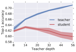
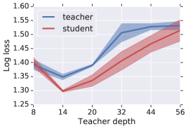
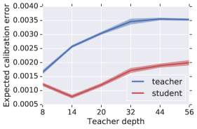
Contribution (i) gives a statistical perspective on the value of “dark knowledge”: for an example $(x,y)$, the logits on “wrong” labels $y^{\prime}\neq y$ encode information about the underlying data distribution. This view elucidates how a teacher’s probability calibration rather than accuracy can influence a student’s generalisation; see Figure 1 for an illustration. Contribution (ii) shows a practical benefit of this statistical view of distillation, by showing how multiclass retrieval objectives benefit from approximate class-probabilities.

(a) Top-1 accuracy.

(b) Log-loss.

(c) Expected calibration error.

Figure 1: Illustration of how better teacher modelling of underlying (Bayes) class-probabilities influences student generalisation, per our statistical perspective. Here, we train ResNets of varying depths on the CIFAR-100 dataset, and use these as teachers to distill to a student ResNet of fixed depth $8$. Figure 1(a) reveals that the teacher model gets increasingly more accurate as its depth increases; however, from 1(b) the corresponding log-loss starts increasing beyond a depth of $14$. The calibration error is also seen to worsen with increasing depth in 1(c). This indicates the teacher’s probability estimates become progressively poorer approximations of the Bayes class-probability distribution $p^{*}(x)$ after certain depth. Intuitively, the teacher’s approximation of $p^{*}$ is governed by balancing the bias and variance in its predictions. The accuracy of the student model also degrades beyond a teacher depth of $14$, reflecting the bound in Proposition 3. See §5.2 for more details, and §3.2 for illustration of a general bias-variance tradeoff.

2 Background and notation

We review multiclass classification, retrieval, & distillation.

2.1 Multiclass classification

In multiclass classification, we are given a training sample $S\stackrel{{\scriptstyle.}}{{=}}\{(x_{n},y_{n})\}_{n=1}^{N}\sim\mathbb{P}^{N}$, for unknown distribution $\mathbb{P}$ over instances $\mathscr{X}$ and labels $\mathscr{Y}=[L]\stackrel{{\scriptstyle.}}{{=}}\{1,2,\ldots,L\}$. Our goal is to learn a predictor $f\colon\mathscr{X}\to\mathbb{R}^{L}$ so as to minimise the risk of $f$, i.e., its expected loss for a random instance and label:

$$R(f)\stackrel{{\scriptstyle.}}{{=}}\underset{({x},{y})\sim\mathbb{P}}{\mathbb{E}}\left[\ell({y},f({x}))\right].$$ (1)

Here, $\ell\colon[L]\times\mathbb{R}^{L}\to\mathbb{R}_{+}$ is a loss function, where for label $y\in[L]$ and prediction vector $f(x)\in\mathbb{R}^{L}$, $\ell(y,f(x))$ is the loss incurred for predicting $f(x)$ when the true label is $y$. A canonical example is the softmax cross-entropy loss,

$$\ell(y,f(x))=-f_{y}(x)+\log\left[\sum_{y^{\prime}\in[L]}e^{f_{y^{\prime}}(x)}\right].$$ (2)

We may approximate the risk $R(f)$ via the empirical risk

$$\hat{R}(f;S)\stackrel{{\scriptstyle.}}{{=}}\frac{1}{N}\sum_{n\in[N]}\ell(y_{n},f(x_{n}))=\frac{1}{N}\sum_{n\in[N]}e_{y_{n}}^{\mathrm{T}}\ell(f(x_{n})),$$ (3)

where ${e}_{y}\in\{0,1\}^{L}$ denotes the one-hot encoding of $y\in[L]$ and $\ell(f(x))\stackrel{{\scriptstyle.}}{{=}}\big{(}\ell(1,f(x)),\ldots,\ell(L,f(x))\big{)}\in\mathbb{R}_{+}^{L}$ denotes the vector of losses for each possible label.

In a multiclass retrieval setting, our goal is to ensure that the top-ranked labels in $f(x)\in\mathbb{R}^{L}$ include the true label (Lapin et al., 2018). Formally, we seek to minimise the top-$k$ loss

$$\ell_{\mathrm{ret}(k)}(y,f(x))\stackrel{{\scriptstyle.}}{{=}}\llbracket y\notin\mathrm{top}_{k}(f(x))\rrbracket,$$ (4)

where $\mathrm{top}_{k}(f)$ denotes the top-$k$ highest scoring labels. When $k=1$, this loss reduces to the standard 0-1 error.

2.2 Knowledge distillation

Distillation involves using a “teacher” model to improve the performance of a “student” model (Bucilǎ et al., 2006; Hinton et al., 2015). In the simplest form, one trains the teacher model and obtains class-probability estimator ${p}^{\mathrm{t}}\colon\mathscr{X}\to\Delta_{\mathscr{Y}}$, where $\Delta$ denotes the simplex. Each ${p}^{\mathrm{t}}_{y}(x)$ estimates how likely $x$ is to be classified as $y$. In place of the empirical risk (3), the student now minimises the distilled risk

$$\tilde{R}(f;S)=\frac{1}{N}\sum_{n\in[N]}{p}^{\mathrm{t}}(x_{n})^{\mathrm{T}}\ell(f(x_{n})),$$ (5)

so that the one-hot encoding of labels is replaced with the teacher’s distribution over labels. Distillation may be used when the student has access to a large pool of unlabelled samples; in this case, distillation is a means of semi-supervised learning (Radosavovic et al., 2018).

While originally conceived in settings where the student has lower capacity than the teacher (Bucilǎ et al., 2006; Hinton et al., 2015), distillation has proven useful when both models have the same capacity (Breiman and Shang, 1996; Furlanello et al., 2018; Xie et al., 2019). More precisely, distillation involves training a teacher on $N_{t}$ labelled samples $S^{\mathrm{t}}\sim\mathbb{P}^{N^{\mathrm{t}}}$, using a function class $\mathscr{F}^{\mathrm{t}}$. Classic distillation assumes that $N^{\mathrm{t}}\gg N$, and that the capacity of $\mathscr{F}^{\mathrm{t}}$ is greater than that of $\mathscr{F}$. “Born-again” distillation assumes that $S^{\mathrm{t}}=S$, and $\mathscr{F}^{\mathrm{t}}=\mathscr{F}$, i.e., one iteratively trains versions of the same model, using past predictions to improve performance.

2.3 Existing explanations for distillation

While it is well-accepted that distillation is empirically useful, there is less consensus as to why this is the case. Hinton et al. (2015) attributed the success of distillation (at least in part) to the encoding of “dark knowledge” in the probabilities the teacher assigns to the “wrong” labels $y^{\prime}\neq y$ for example $(x,y)$. This richer information plausibly aids the student, providing for example a weighting on the samples (Furlanello et al., 2018; Tang et al., 2020). Further, when $\ell$ is the softmax cross-entropy, the gradient of the distillation objective with respect to the student logits is the difference in the probability estimates for the two, implying a form of logit matching in high-temperature regimes (Hinton et al., 2015).

Lopez-Paz et al. (2016) related distillation to learning from privileged information under a noise-free setting.  Phuong and Lampert (2019) analysed the dynamics of student learning, assuming a deep linear model for binary classification.  Foster et al. (2019) provided a generalisation bound for the student, under the assumption that it learns a model close to the teacher. This does not, however, explicate what constitutes an “ideal” teacher, nor quantify how an approximation to this ideal teacher will affect the student generalisation. Gotmare et al. (2019) studied the effect of distillation on discrimination versus feature extraction layers of the student network. (Dong et al., 2019) argued that distillation has a similar effect to early stopping, and studied its ability to denoise labels. Our focus, by contrast, is in settings where there is no exogenous label noise, and in studying the statistical rather than optimisation effects of distillation. (Mobahi et al., 2020) analysed the special setting of self-distillation – wherein the student and teacher employ the same model class – and showed that for kernelised models, this is equivalent to increasing the regularisation strength.

3 Distillation through a class-probability lens

We now present a statistical perspective of distillation, which gives insight into why it can aid generalisation. Central to our perspective are two observations:

1. the risk (1) we seek to minimise inherently smooths labels by the class-probability distribution $\mathbb{P}(y\mid x)$;

2. a teacher’s predictions provide an approximation to the class-probability distribution $\mathbb{P}(y\mid x)$, which can thus yield a better approximation to the risk (1) than one-hot labels.

Building on these, we show how sufficiently accurate teacher approximations can improve student generalisation.

3.1 Bayes knows best: distilling class-probabilities

Our starting point is the following elementary observation: the underlying risk $R(f)$ for a predictor $f\colon\mathscr{X}\to\mathbb{R}^{L}$ is

$$R(f) =\underset{{x}}{\mathbb{E}}\left[\underset{{y}\mid{x}}{\mathbb{E}}\left[\ell({y},f({x}))\right]\right]$$

$$=\underset{{x}}{\mathbb{E}}\left[p^{*}({x})^{\mathrm{T}}\ell(f({x}))\right],$$ (6)

where $p^{*}(x)\stackrel{{\scriptstyle.}}{{=}}\begin{bmatrix}\mathbb{P}(y\mid x)\end{bmatrix}_{y\in[L]}\in\Delta_{\mathscr{Y}\stackrel{{\scriptstyle.}}{{=}}[L]}$ is the Bayes class-probability distribution. Intuitively, $\mathbb{P}(y\mid x)$ inherently captures the suitability of label $y$ for instance $x$. Thus, the risk involves drawing an instance ${x}\sim\mathbb{P}({{x}})$, and then computing the average loss of $f({x})$ over all labels $y\in[L]$, weighted by their Bayes probabilities $\mathbb{P}(y\mid x)$. When $p^{*}(x)$ is not concentrated on a single label, there is an inherent confusion amongst the labels for the instance $x$.

Given an $(x_{n},y_{n})\sim\mathbb{P}$, the empirical risk (3) approximates the distribution $p^{*}(x_{n})$ with the one-hot $e_{y_{n}}$, which is only supported on one label. While this is an unbiased estimate, it is a significant reduction in granularity. By contrast, consider the following Bayes-distilled risk on a sample $S\sim\mathbb{P}^{N}$:

$$\hat{R}_{*}(f;S)\stackrel{{\scriptstyle.}}{{=}}\frac{1}{N}\sum_{n=1}^{N}p^{*}(x_{n})^{\mathrm{T}}\ell(f(x_{n})).$$ (7)

This is a distillation objective (cf. (5)) using a Bayes teacher, who provides the student with the true class-probabilities. Rather than fitting to a single label realisation $y_{n}\sim p^{*}(x_{n})$, a student minimising (7) considers all alternate label realisations, weighted by their likelihood. Observe that when $\ell$ is the cross-entropy, (7) is simply the KL divergence between the Bayes class-probabilities and our predictions.

Both the standard empirical risk $\hat{R}(f;S)$ in (3) and Bayes-distilled risk $\hat{R}_{*}(f;S)$ in (7) are unbiased estimates of the population risk $R(f)$. But intuitively, we expect that a student minimising (7) ought to generalise better from a finite sample. We can make this intuition precise by establishing that the Bayes-distilled risk has lower variance, considering fresh draws of the training sample.

Lemma 1.

For any fixed predictor $f\colon\mathscr{X}\to\mathbb{R}^{L}$,

$$\mathbb{V}_{S\sim\mathbb{P}^{N}}\left[\hat{R}_{*}(f;S)\right]\leq\mathbb{V}_{S\sim\mathbb{P}^{N}}\left[\hat{R}(f;S)\right],$$

where $\mathbb{V}$ denotes variance, and equality holds iff $\forall x\in\mathscr{X}$, the loss values $\ell(f(x))$ are constant on the support of $p^{*}(x)$.

Proof of Lemma 1.

By definition,

$$\mathrm{LHS} =\frac{1}{N}\cdot\mathbb{V}\left[p^{*}({x})^{\mathrm{T}}\ell(f({x}))\right]$$

$$=\frac{1}{N}\cdot\mathbb{V}\left[\underset{{y}\mid{x}}{\mathbb{E}}\left[\ell({y},f({x}))\right]\right]$$

$$=\frac{1}{N}\cdot\underset{{x}}{\mathbb{E}}\,\left[\underset{{y}\mid{x}}{\mathbb{E}}\left[\ell({y},f({x}))\right]\right]^{2}-\frac{1}{N}\cdot\left[\underset{{x}}{\mathbb{E}}\,\underset{{y}\mid{x}}{\mathbb{E}}\left[\ell({y},f({x}))\right]\right]^{2}.$$

$$\mathrm{RHS} =\frac{1}{N}\cdot\mathbb{V}\left[\ell({y},f({x}))\right]$$

$$=\frac{1}{N}\cdot\underset{{x}}{\mathbb{E}}\,\underset{{y}\mid{x}}{\mathbb{E}}\left[\ell({y},f({x}))^{2}\right]-\frac{1}{N}\cdot\left[\underset{{x}}{\mathbb{E}}\,\underset{{y}\mid{x}}{\mathbb{E}}\left[\ell({y},f({x}))\right]\right]^{2}.$$

In both cases, the second term simply equals $R(f)^{2}$ since both estimates are unbiased. For fixed $x\in\mathscr{X}$, the result follows by Jensen’s inequality applied to the random variable $Z\stackrel{{\scriptstyle.}}{{=}}\ell({y},f(x))$. Equality occurs iff $Z$ is constant, which requires the loss to be constant on the support of $p^{*}(x)$. ∎

The condition when the Bayes-distilled and empirical risks have the same variance is intuitive: the two risks trivially agree when $f$ is non-discriminative (attaining equal loss on all labels), or when a label is inherently deterministic (the class-probability is concentrated on one label). For discriminative predictors and non-deterministic labels, however, the Bayes-distilled risk can have significantly lower variance.

The reward of reducing variance is better generalisation: a student minimising (7), will better minimise the population risk, compared to using one-hot labels. In fact, we may quantify how the empirical variance of the Bayes-distilled loss values influences generalisation as follows.

Proposition 2.

Pick any bounded loss $\ell$. Fix a hypothesis class $\mathscr{F}$ of predictors $f\colon\mathscr{X}\to\mathbb{R}^{L}$, with induced class $\mathscr{H}^{*}\subset[0,1]^{\mathscr{X}}$ of functions $h(x)\stackrel{{\scriptstyle.}}{{=}}p^{*}(x)^{\mathrm{T}}\ell(f(x))$. Suppose $\mathscr{H}^{*}$ has uniform covering number $\mathscr{N}_{\infty}$. Then, for any $\delta\in(0,1)$, with probability at least $1-\delta$ over $S\sim\mathbb{P}^{N}$,

$$R(f)\leq\hat{R}_{*}(f;S)+\mathscr{O}\left(\sqrt{\mathbb{V}^{*}_{N}(f)\cdot\frac{\log\frac{\mathscr{M}^{*}_{N}}{\delta}}{N}}+\frac{\log\frac{\mathscr{M}^{*}_{N}}{\delta}}{N}\right),$$

where $\mathscr{M}^{*}_{N}\stackrel{{\scriptstyle.}}{{=}}\mathscr{N}_{\infty}(\frac{1}{N},\mathscr{H}^{*},2N)$ and $\mathbb{V}^{*}_{N}(f)$ is the empirical variance of the loss values $\{p^{*}(x_{n})^{\mathrm{T}}\ell(f(x_{n}))\}_{n=1}^{N}$.

Proof of Proposition 2.

This a simple consequence of Maurer and Pontil (2009, Theorem 6), which is a uniform convergence version of Bennet’s inequality (Bennett, 1962). ∎

The above may be contrast to the bound achievable for the standard empirical risk using one-hot labels: by Maurer and Pontil (2009, Theorem 6),

$$R(f)\leq\hat{R}(f;S)+\mathscr{O}\left(\sqrt{\mathbb{V}_{N}(f)\cdot\frac{\log\frac{\mathscr{M}_{N}}{\delta}}{N}}+\frac{\log\frac{\mathscr{M}_{N}}{\delta}}{N}\right),$$

where here we consider a function class $\mathscr{H}$ comprising functions $h(x,y)=e_{y}^{\mathrm{T}}\ell(f(x))$, with uniform covering number $\mathscr{M}_{N}$. Combining the above with Lemma 1, we see that the Bayes-distilled empirical risk results in a lower variance penalty.

To summarise the statistical perspective espoused above, a student should ideally have access to the underlying class-probabilities $p^{*}(x)$, rather than a single realisation $y\sim p^{*}(x)$. As a final comment, the above provides a statistical perspective on the value of “dark knowledge”: the teacher’s “wrong” logits $y^{\prime}\neq y$ for an example $(x,y)$ provide approximate information about the Bayes class-probabilities. This results in a lower-variance student objective, aiding generalisation.

3.2 Distilling from an imperfect teacher

The previous section explicates how an idealised “Bayes teacher” can be beneficial to a student. How does this translate to more realistic settings, where one obtains predictions from a teacher which itself is learned form data?

Our first observation is that a teacher’s predictor ${p}^{\mathrm{t}}$ can typically be seen as an imperfect estimate of the true $p^{*}$. Indeed, if the teacher is trained with a loss that is proper (Savage, 1971; Schervish, 1989; Buja et al., 2005), then

$$R(f)=\underset{{x}}{\mathbb{E}}\left[D(p^{*}({x})\|{p}^{\mathrm{t}}({x}))\right]+\mathrm{constant},$$ (8)

where $D(\cdot\|\cdot)$ is a (loss-dependent) divergence between the true and estimated class-probability functions. For example, the softmax cross-entropy corresponds to $D(\cdot\|\cdot)$ being the KL divergence between the distributions. The teacher’s goal is thus fundamentally to ensure that their predictions align with the true class-probability function.

Of course, a teacher learned from finite samples is unlikely to achieve zero divergence in (8). Indeed, even high-capacity teacher models may not be rich enough capture the true $p^{*}$. Further, even if the teacher can represent $p^{*}$, it may not be able to learn this perfectly given a finite sample, owing to both statistical (e.g., the risk of overfitting) and optimisation (e.g., non-convexity of the objective) issues. We must thus treat ${p}^{\mathrm{t}}$ as an imperfect estimate of $p^{*}$. The natural question is: will such an estimate still improve generalisation?

To answer this, we establish a fundamental bias-variance tradeoff when performing distillation. Specifically, we show the difference between the distilled risk $\tilde{R}(f;S)$ (cf. (5)) and population risks $R(f)$ (cf. (3.1)) depends on how variable the loss under the teacher is, and how well the teacher estimates $p^{*}$ in a squared-error sense. Intuitively, the latter captures how well the teacher estimates $p^{*}$ on average (bias), and how variable the teacher’s predictions are (variance).

Proposition 3.

Pick any bounded loss $\ell$. Suppose we have a teacher model ${p}^{\mathrm{t}}$ with corresponding distilled empirical risk in (5). For constant $C>0$ and any predictor $f\colon\mathscr{X}\to\mathbb{R}^{L}$,

$$\underset{}{\mathbb{E}}\left[(\tilde{R}(f;S)-R(f))^{2}\right] \leq\frac{1}{N}\cdot\mathbb{V}\left[{p}^{\mathrm{t}}({x})^{\mathrm{T}}\ell(f({x}))\right]+C\cdot\left(\underset{}{\mathbb{E}}\left[\|{p}^{\mathrm{t}}({x})-p^{*}({x})\|_{2}\right]\right)^{2}$$ (9)

$$\leq\frac{1}{N}\cdot\mathbb{V}\left[{p}^{\mathrm{t}}({x})^{\mathrm{T}}\ell(f({x}))\right]+C\cdot\left({\|\underset{}{\mathbb{E}}\left[{p}^{\mathrm{t}}({x})\right]-p^{*}({x})\|_{2}^{2}}+\mathbb{V}\left[{p}^{\mathrm{t}}({x})\right]\right),$$ (10)

where $\mathbb{V}\left[\cdot\right]$ denotes the sum of coordinate-wise variance.

Proof of Proposition 3.

Let $\Delta\stackrel{{\scriptstyle.}}{{=}}\tilde{R}(f;S)-R(f)$. Then,

$$\underset{}{\mathbb{E}}\left[(\tilde{R}(f;S)-R(f))^{2}\right] =\underset{}{\mathbb{E}}\left[\Delta^{2}\right]=\mathbb{V}[\Delta]+\underset{}{\mathbb{E}}\left[\Delta\right]^{2}.$$

Observe that

$$\underset{}{\mathbb{E}}\left[\Delta\right] =\underset{{x}}{\mathbb{E}}\left[({p}^{\mathrm{t}}({x})-p^{*}({x}))^{\mathrm{T}}\ell(f({x}))\right]$$

$$\leq\underset{{x}}{\mathbb{E}}\left[\|{p}^{\mathrm{t}}({x})-p^{*}({x})\|_{2}\cdot\|\ell(f({x}))\|_{2}\right]$$

$$\leq\underset{{x}}{\mathbb{E}}\left[\|{p}^{\mathrm{t}}({x})-p^{*}({x})\|_{2}\cdot C\cdot\|\ell(f({x}))\|_{\infty}\right]$$

$$\leq C\cdot\underset{{x}}{\mathbb{E}}\left[\|{p}^{\mathrm{t}}({x})-p^{*}({x})\|_{2}\right],$$

where the second line is by the Cauchy-Schwartz inequality, and the third line by the equivalence of norms. Now, (9) follows since $R(f)$ is a constant, implying

$$\mathbb{V}[\Delta] =\mathbb{V}[\tilde{R}(f;S)]=\frac{1}{N}\cdot\mathbb{V}\left[{p}^{\mathrm{t}}({x})^{\mathrm{T}}\ell(f({x}))\right].$$

For (10), by Jensen’s inequality, and the definition of variance,

$$\left(\underset{{x}}{\mathbb{E}}\left[\|{p}^{\mathrm{t}}({x})-p^{*}({x})\|_{2}\right]\right)^{2} \leq\underset{{x}}{\mathbb{E}}\left[\|{p}^{\mathrm{t}}({x})-p^{*}({x})\|_{2}^{2}\right]$$

$$=\|\underset{}{\mathbb{E}}\left[{p}^{\mathrm{t}}({x})\right]-p^{*}({x})\|_{2}^{2}+\mathbb{V}\left[{p}^{\mathrm{t}}({x})\right].$$

∎

Unpacking the above, the fidelity of the distilled risk’s approximation to the true one depends on three factors: how variable the expected loss is for a random instance; how well the teacher’s ${p}^{\mathrm{t}}$ approximates the true $p^{*}$ on average; and how variable the teacher’s predictions are. Mirroring the previous section, we may convert Proposition 3 into a generalisation bound for the student:

$$R(f)\leq\tilde{R}(f;S)+\mathfrak{C}(\mathscr{F},N)+\mathscr{O}\left(\mathbb{E}{}{\|{p}^{\mathrm{t}}({x})-p^{*}({x})\|_{2}}\right),$$ (11)

where $\mathfrak{C}$ is the penalty term from Proposition 2. As is intuitive, using an imperfect teacher invokes an additional penalty depending on how far the predictions are from the Bayes, in a squared-error sense. For completeness, a formal statement is provided in Proposition 5 in Appendix A.

3.3 Discussion and implications

Our statistical perspective gives a simple yet powerful means of understanding distillation. Our formal results follow readily from this perspective, but their implications are subtle, and merit further discussion.

$\triangleright$ Why accuracy is not enough. Our bias-variance result establishes that if the teacher provides good class-probabilities, in the sense of approximating $p^{*}$ in a mean-square sense, then the resulting student should generalise well. In deep networks, this does not imply providing the teacher having higher accuracy; such models may be accurate while being overly confident (Guo et al., 2017; Rothfuss et al., 2019). Our result thus potentially illuminates why more accurate teachers may lead to poorer students, as has been noted empirically (Müller et al., 2019); see also §5.2.

In practice, the precise bound derived above is expected to be loose. However, its qualitative trend may be observed in practice. Figure 1 (see also §5.2) illustrates how increasing the depth of a ResNet model may increase accuracy, but degrade probabilistic calibration. This is seen to directly relate to the quality of a student distilled from these models.

Temperature scaling (Hinton et al., 2015), a very common and empirically successful trick in distillation, can also be analysed through this perspective. Usually, teachers are highly complex and optimised to maximise accuracy; hence, they often become overly confident. Increasing the temperature can help the student-target be closer to the true distribution, and not just convey the most accurate label.

$\triangleright$ Teacher variance and model capacity. Proposition 3 allows for ${p}^{\mathrm{t}}$ to be random (e.g., owing to the teacher being learned from some independent sample $S^{\mathrm{t}}\sim\mathbb{P}^{N^{\mathrm{t}}}$). Consequently, the variance terms not only reflect how diffused the teacher’s predictions are, but also how much these predictions vary over fresh draws of the teacher sample. High-capacity teachers may yield vastly different predictions when trained on fresh samples. This variability incurs a penalty in the third term in Proposition 3. At the same time, such teachers can better estimate the Bayes $p^{*}(x)$, which incurs a lower bias. The delicate tradeoff between these concerns translates into (student) generalisation.

We may understand the label smoothing trick (Szegedy et al., 2016) in light of the above. This corresponds to mixing the student labels with uniform predictions, yielding ${p}^{\mathrm{t}}(x)=(1-\alpha)\cdot e_{y}+\frac{\alpha}{L}\cdot\mathbf{1}$ for $\alpha\in[0,1]$. From the perspective of modelling $p^{*}$, choosing $\alpha>0$ introduces a bias. However, ${p}^{\mathrm{t}}(x)$ has lower variance than the one-hot labels $e_{y}$’s, owing to the $(1-\alpha)$ scaling. Provided the bias is not too large, smoothing can thus aid generalisation.

We remark also that the first variance term in Proposition 3 vanishes as $N\to\infty$. This is intuitive: in the limit of infinite student samples, the quality of the distilled objective is wholly determined by how well the teacher probabilities model the Bayes probabilities. For small $N$, this term measures how diffused the losses are when weighted by the teacher probabilities (similar to Lemma 1).

$\triangleright$ How much teacher bias is admissible? When ${p}^{\mathrm{t}}\neq p^{*}$, Proposition 3 reveals that a distilled student’s generalisation gap depends on the bias and variance in ${p}^{\mathrm{t}}$. By contrast, from a labelled sample, the student’s generalisation gap depends on the complexity of its model class $\mathscr{F}$. Distillation can be expected to help when the first gap is lower than the second.

Concretely, when trained from limited labelled samples, the student will find $\min_{f\in\mathscr{F}}\hat{R}(f;S)$, which incurs a high statistical error. Now suppose we have a large amount of unlabelled data $N\to\infty$. A distilled student can then reliably find the minimiser (following (8))

$$\min_{f\in\mathscr{F}}\underset{{x}}{\mathbb{E}}\left[D({p}^{\mathrm{t}}({x})\|f({x}))\right],$$

with essentially no statistical error, but an approximation error given by the teacher’s bias. In this setting, we thus need the teacher’s bias to be lower than the statistical error.

$\triangleright$ On teacher versus student samples A qualifier to our results is that they assume a disjoint set of samples for the teacher and student. For example, it may be that the teacher is trained on a pool of labelled samples, while the student is trained on a larger pool of unlabelled samples. The results thus do not directly hold for the settings of self- or co-distillation (Furlanello et al., 2018; Anil et al., 2018), wherein the same sample is used for both models. Combining our results with recent analyses from the perspective of regularisation (Mobahi et al., 2020) and data-dependent function classes (Foster et al., 2019) would be of interest in future work.

4 Distillation meets multiclass retrieval

Our statistical view has thus far given insight into the potential value of distillation. We now show a distinct practical benefit of this view, by leveraging it for a novel application of distillation to multiclass retrieval. Our basic idea is to construct a double-distillation objective, wherein distillation informs the loss as to the relative confidence of both “positive” and “negative” labels.

4.1 Double-distillation for multiclass retrieval

Recall from (4) that in multiclass retrieval, we wish to ensure that the top-ranked labels in our predictor $f(x)\in\mathbb{R}^{L}$ contain the true label. The softmax-cross entropy $\ell(y,f(x))$ in (2) offers a reasonable surrogate loss for this task, since

$$\lim_{\gamma\to 0}\frac{1}{\gamma}\cdot\log\left[\sum_{y^{\prime}\in[L]}e^{\gamma\cdot(f_{y^{\prime}}(x)-f_{y}(x))}\right]=\max_{y^{\prime}\neq y}f_{y^{\prime}}(x)-f_{y}(x).$$

The latter is related to the Cramer-Singer loss (Crammer and Singer, 2002), which bounds the top-$1$ retrieval loss. Given a sample $\{(x_{n},y_{n})\}_{n=1}^{N}$, we thus seek to minimise $\ell(y_{n},f(x_{n}))$. From our statistical view, there is value in instead computing $p^{*}(x_{n})^{\mathrm{T}}\ell(f(x_{n}))$: intuitively, each $y\in[L]$ acts a “smooth positive”, weighted by the Bayes probability $p^{*}_{y}(x_{n})$.

We observe, however, that such smoothing does not affect the innards of the loss itself. In particular, one critique of (2) is that it assigns equal importance to each $y^{\prime}\in[L]$. Intuitively, mistakes on labels $y^{\prime}$ that are a poor explanation for $x$ — i.e., have low $p^{*}_{y^{\prime}}(x)$ — ought to be strongly penalised. On the other hand, if under the Bayes probabilities some $y^{\prime}\neq y$ strongly explains $x$, it ought to be ignored.

To this end, consider a generalised softmax cross-entropy:

$$\ell(y,f(x))\stackrel{{\scriptstyle.}}{{=}}\log\underset{{y}^{\prime}\sim P(x)}{\mathbb{E}}\left[e^{f_{{y}^{\prime}}({x})-f_{y}({x})}\right],$$ (12)

where $P(x)\in\Delta_{L}$ is a distribution over labels. When $P(x)$ is uniform, this is exactly the standard cross-entropy loss (cf. (2)) plus a constant. For non-uniform $P(x)$, however, the loss is encouraged to focus on ensuring $f_{y}(x)\gg f_{y^{\prime}}(x)$ for those $y^{\prime}$ with large $P_{y^{\prime}}(x)$.

Continuing our statistical view, we posit that an ideal choice of $P$ is $P(x)=\Psi(p^{*}(x))$, where $\Psi(\cdot)$ is some decreasing function. Concretely, our new loss for a given $(x,y)$ is

$$\ell(y,f(x))=\log\sum_{y^{\prime}\in[L]}\Psi(p^{*}_{y^{\prime}}(x))\cdot e^{f_{y^{\prime}}(x)-f_{y}(x)}.$$

Intuitively, the loss treats $y$ as a “positive” label for $x$, and each $y^{\prime}\in[L]$ where $y^{\prime}\neq y$ as a “negative” label. The loss seeks to score the positive label over all labels which poorly explain $x$. Compared to the standard softmax cross-entropy, we avoid penalisation when $y^{\prime}$ plausibly explains $x$ as well.

Recall that under a distillation setup, a teacher model provides us estimates ${p}^{\mathrm{t}}(x)$ of $p^{*}(x)$. Consequently, to estimate this risk on a finite sample $S=\{(x_{n},y_{n})\}_{n=1}^{N}$, we may construct the following double-distillation objective:

$$\tilde{R}(f;S) =\frac{1}{N}\sum_{n=1}^{N}{p}^{\mathrm{t}}(x_{n})^{\mathrm{T}}\ell(f(x_{n}))$$ (13)

$$\ell(y,f(x_{n})) =\log\left[\overline{{p}^{\mathrm{t}}}(x_{n})^{\mathrm{T}}e^{f(x_{n})-f_{y}(x_{n})}\right],$$

where $\overline{{p}^{\mathrm{t}}}(x)\stackrel{{\scriptstyle.}}{{=}}\Psi({{p}^{\mathrm{t}}}(x))$; unrolling, this corresponds to the objective

$$\tilde{R}(f;S)=\frac{1}{N}\sum_{n=1}^{N}\sum_{y\in[L]}{p}^{\mathrm{t}}(y\mid x_{n})\cdot\log\left[\sum_{y^{\prime}\in[L]}\overline{{p}^{\mathrm{t}}}(y^{\prime}\mid x_{n})\cdot e^{f_{y^{\prime}}(x_{n})-f_{y}(x_{n})}\right].$$

Observe that (13) uses the teacher in two ways: the first is the standard use of distillation to smooth the “positive” training labels. The second is a novel use of distillation to smooth the “negative” labels. Here, for any candidate “positive” label $y$, we apply varying weights to “negative” labels $y^{\prime}\neq y$ when computing each $\ell(y,f(x))$.

It remains to specify the precise form of $\Psi(\cdot)$ in (13). A natural choice of $1-{p}^{\mathrm{t}}(x)$; however, since the entries of ${p}^{\mathrm{t}}(x)$ sum to one, this may not allow the loss to sufficiently ignore other “positive” labels. Concretely, suppose there are $L^{+}$ plausible “positive” labels, which have most of the probability mass under ${p}^{\mathrm{t}}(x)$. Then, the total weight assigned to these labels will be roughly $L^{+}-1$; this is of the order of $L^{+}$, which is what we would get from uniform weights.

To resolve this, we may instead use weights proportional to $1-\sigma(a\cdot s_{y}(x))$, where $\sigma(\cdot)$ is the sigmoid function, $s_{y}(x)$ is the teacher logit, and $a>0$ is a scaling parameter which may be tuned. This parameterisation allows for multiple labels to have high (or low) weights. In the above example, each “positive” label can individually get a score close to $0$. The total weight of the “positives” can thus also be close to $0$, and so the loss can learn to ignore them.

4.2 Discussion and implications

The viability of distillation as a means of smoothing negatives has not, to our knowledge, been explored in the literature. The proposal is, however, a natural consequence of our statistical view of distillation developed in §3.

The double-distillation objective in (13) relates to ranking losses. In bipartite ranking settings (Cohen et al., 1999), one assumes an instance space $\mathscr{X}$ and binary labels $\mathscr{Y}=\{0,1\}$ denoting that items are either relevant, or irrelevant. Rudin (2009) proposed the following push loss for this task:

$$R_{\mathrm{push}}(h) \stackrel{{\scriptstyle.}}{{=}}\underset{z\sim\mathbb{P}_{+}}{\mathbb{E}}\left[g\left(\underset{z^{\prime}\sim\mathbb{P}_{-}}{\mathbb{E}}\left[\phi(h(z^{\prime})-h(z))\right]\right)\right]$$

where $\mathbb{P}_{+}$ and $\mathbb{P}_{-}$ are distributions over positive and negative instances respectively, and $g(\cdot),\phi(\cdot)$ are convex non-decreasing functions. Similar losses have also been studied in Yun et al. (2014). The generalised softmax cross-entropy in (12) can be seen as a contextual version of this objective for each $x\in\mathscr{X}$, where $g(z)=\log(1+z)$ and $\phi(z)=e^{-z}$. In double-distillation, the contextual distributions $\mathbb{P}_{\pm}(x)$ are approximated using the teacher’s predictions ${p}^{\mathrm{t}}(x)$.

There is a broad literature on using a weight on “negatives” in the softmax (Liu et al., 2016, 2017; Wang et al., 2018; Li et al., 2019; Cao et al., 2019); this is typically motivated by ensuring a varying margin for different classes. The resulting weighting is thus either constant or label-dependent, rather than the label- and example-dependent weights provided by distillation. Closer still to our framework is the recent work of Khan et al. (2019), which employs uncertainty estimates in the predictions for a given example and label to adjust the desired margin in the softmax. While not explicitly couched in terms of distillation, this may be understood as a “self-distillation” setup, wherein the current predictions of a model are used to progressively refine future iterates. Compared to double-distillation, however, the nature of the weighting employed is considerably more complicated.

There is a rich literature on the problem of label ranking, where typically it is assumed that one observes a (partial) ground-truth ranking over labels (Dekel et al., 2003; Fürnkranz et al., 2008; Vembu and Gärtner, 2011). We remark also that the view of the softmax as a ranking loss has received recent attention (Bruch et al., 2019; Bruch, 2019). Exploiting the statistical view of distillation in these regimes is a promising future direction. Tang and Wang (2018) explored distillation in a related learning-to-rank framework. While similar in spirit, this focusses on pointwise losses, wherein the distinction between positive and negative smoothing is absent.

Finally, we note that while our discussion has focussed on the softmax cross-entropy, double-distillation may be useful for a broader class of losses, e.g., order-weighted losses as explored in Usunier et al. (2009); Reddi et al. (2019).

5 Experimental results

We now present experiments illustrating three key points:

1. we show that distilling with true (Bayes) class-probabilities improves generalisation over one-hot labels, validating our statistical view of distillation.

2. we illustrate our bias-variance tradeoff on synthetic and real-world datasets, confirming that teachers with good estimates of $p^{*}$ can be usefully distilled.

3. we finally show that double-distillation performs well on real-world multiclass retrieval datasets, confirming the broader value in our statistical perspective.

(a) Student AUC versus # of training samples.

(b) Student AUC versus class separation.

Figure 2: Distillation with Bayes-teacher on synthetic data comprising Gaussian class-conditionals. Distillation offers a noticeable gain over the standard one-hot encoding, particularly in the small-sample regime (left), and when the underlying problem is noisier (right).

5.1 Is Bayes a good teacher for distillation?

To illustrate our statistical perspective, we conduct a synthetic experiment where $p^{*}(x)$ is known, and show that distilling these Bayes class-probabilities benefits learning.

We generate training samples $S=\{(x_{n},y_{n})\}_{i=1}^{N}$ from a distribution $\mathbb{P}$ comprising class-conditionals which are each 10-dimensional Gaussians, with means $\pm(1,1,\ldots,1)$ respectively. By construction, the Bayes class-probability distribution is $p^{*}(x)=(\mathbb{P}(y=0\mid x),\mathbb{P}(y=1\mid x))$ where $\mathbb{P}(y=1\mid x)=\sigma((\theta^{*})^{\mathrm{T}}x)$, for $\theta^{*}\stackrel{{\scriptstyle.}}{{=}}(2,2,\ldots,2)$.

We compare two training procedures: standard logistic regression on $S$, and Bayes-distilled logistic regression using $p^{*}(x_{n})$ per (7). Logistic regression is well-specified for this problem, i.e., as $N\to\infty$, the standard learner will learn $\theta^{*}$. However, we will demonstrate that on finite samples, the Bayes-distilled learner’s knowledge of $p^{*}(x_{n})$ will be beneficial. We reiterate that while this learner could trivially memorise the training $p^{*}(x_{n})$, this would not generalise.

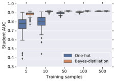
Figure 2(a) compares the performance of these two approaches for varying training set sizes, where for each training set size we perform $100$ independent trials and measure the AUC-ROC on a test set of $10^{4}$ samples. We observe two key trends: first, Bayes-distillation generally offers a noticeable gain over the standard one-hot encoding, in line with our theoretical guarantee of low variance.

Second, both methods see improved performance with more samples, but the gains are greater for the one-hot encoding. This in line with our intuition that distillation effectively augments each training sample: when $N$ is large to begin with, the marginal gain of such augmentation is minimal.

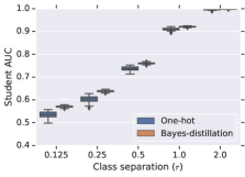
Figure 2(b) continues the exploration of this setting. We now vary the distance $r$ between the means of each of the Gaussians. When $r$ is small, the two distributions grow closer together, making the classification problem more challenging. We thus observe that both methods see worse performance as $r$ is smaller. At the same time, smaller $r$ makes the one-hot labels have higher variance compared to the Bayes class-probabilities. Consequently, the gains of distillation over the one-hot encoding are greater for this setting, in line with our guarantee on the lower-variance Bayes-distilled risk aiding generalisation (Proposition 2).

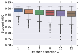
As a final experiment, we verify the claim that teacher accuracy does not suffice for improving student generalisation, since this does not necessarily correlate with the quality of the teacher’s probability estimates. We assess this by artificially distorting the teacher probabilities so as to perfectly preserve teacher accuracy, while degrading their approximation to $p^{*}$. Appendix B.2 presents plots confirming that such degradation progressively reduces the gains of distillation.

5.2 Illustration of bias-variance tradeoff

We next illustrate our analysis on the bias-variance tradeoff in distillation from §3.2 on synthetic and real-world datasets.

Synthetic. We now train a series of increasingly complex teacher models ${p}^{\mathrm{t}}$, and assess their resulting distillation benefit on a synthetic problem. Here, the data is sampled from a marginal $\mathbb{P}(x)$ which is a zero-mean isotropic Gaussian in 2D. The class-probability function is given by $\eta(x)=\sigma(2\cdot(\|x\|_{\infty}-0.5))$, so that the negatives are concentrated in a rectangular slab.

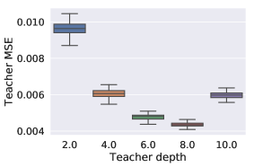
We consider teachers that are random forests of a fixed depth $d\in\{1,2,4,8,16\}$, with $3$ base estimators. Increasing $d$ has the effect of reducing teacher bias (since the class of depth-$d$ trees can better approximate $p^{*}$), but increasing teacher variance (since the class of depth-$d$ trees can induce complex decision boundaries). For fixed $d$, we train a teacher model on the given training sample $S$ (with $N=100$). We then distill the teacher predictions to a student model, which is a depth $4$ tree. For each such teacher, we compute its MSE, as well as the test set AUC of the corresponding distilled student. We repeat this for $100$ independent trials.

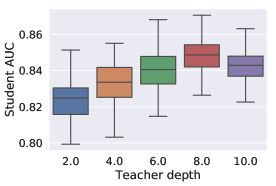
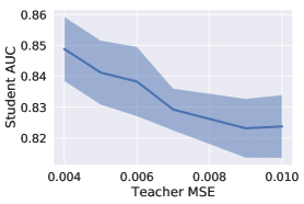
Figure 3(a) and 3(b) show how the teacher’s depth affects its MSE in modelling $p^{*}$, as well as the AUC of the resulting distilled student. There is an optimal depth $d=8$ at which the teacher achieves the best MSE approximation of $p^{*}$. In keeping with the theory, this also corresponds to the teacher whose resulting student generalises the best. Figure 4(a) combines these plots to explicitly show the relationship between the the teacher’s MSE and the student’s AUC. In line with the theory, more accurate estimates of $p^{*}$ result in better students.

Note that at depth $10$, the teacher model is expected to have lower bias; however, it results in a slightly worse distilled student. This verifies that one may favour a higher-bias teacher if it has lower variance: a teacher may achieve a lower MSE – and thus distill better – by slightly increasing its bias while lowering variance. See Appendix B.1 for additional bias-variance experiments on synthetic data.

Fashion MNIST. It is challenging to assess the bias-variance tradeoff on real-world datasets, where the Bayes $p^{*}(x)$ is unknown. As a proxy, we take the fashion MNIST dataset, and treat a powerful teacher model as our $p^{*}$. We train an MLP teacher with two hidden layers with $128$ and $10$ dimensions. This achieves a test accuracy of $\sim 89\%$.

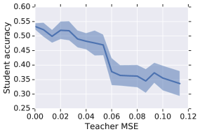
We then inject bias and noise per (16), and distill the result to a linear logistic regression model. To amplify the effects of distillation, we constrain the student by only offering it the top $2500$ samples that the original teacher deems most uncertain. Figures 4(b) demonstrates similar trend to the synthetic dataset, with the best MSE approximator to the original teacher generally yielding the best student.

CIFAR-100. We verify that accurate probabilty estimation by the teacher strongly influences student generalisation, and that this can be at odds with accuracy. We revisit the plots introduced in Figure 1. Here, we train ResNets of varying depths on the CIFAR-100 dataset, and use these as teachers to distill to a student ResNet of fixed depth $8$. Figure 1(a) reveals that the teacher model gets increasingly more accurate as its depth increases; however, the corresponding log-loss starts increasing beyond a depth of $14$. This indicates the teacher’s probability estimates become progressively poorer approximations of the Bayes class-probability distribution $p^{*}(x)$. The accuracy of the student model also degrades beyond a teacher depth of $14$, reflecting the bias-variance bound in Proposition 3.

(a) Teacher depth versus MSE.

(b) Teacher depth versus student AUC.

Figure 3: Relationship between depth of teacher’s decision tree model (model complexity) and its MSE in modelling $p^{*}$, as well as the AUC of the resulting distilled student, on a synthetic problem. There is an optimal depth $d=8$ at which the teacher achieves the best MSE approximation of $p^{*}$. In keeping with the theory, this corresponds to the teacher whose resulting student generalises the best.

(a) Synthetic dataset.

(b) Fashion MNIST dataset.

Figure 4: Relationship between teacher’s MSE against true class-probability and student’s test set AUC. In keeping with the theory, teachers which better approximate $p^{*}$ in an MSE sense yield better students.

5.3 Double-distillation for multiclass retrieval

Our final set of experiments confirm the value in our double-distillation objective in (13). To do so, we use the AmazonCat-13K and Amazon-670K benchmark datasets for multiclass retrieval (McAuley and Leskovec, 2013; Bhatia et al., 2015). The data is multilabel; following Reddi et al. (2019), we make it multiclass by creating a single example $(x,y)$ for each label $y$ associated with $x$.

We construct a “teacher” model using a feedforward network with a single (linear) hidden layer of width $512$, trained to minimise the softmax cross-entropy loss. We then construct a “student” model using the same architecture, but with a hidden layer of width $8$ for AmazonCat-13K and $64$ for Amazon-670K because Amazon-670K is significantly larger than AmazonCat-13K (670k vs 13k labels). This student model is compared to a distilled student, where the teacher logits are used in place of the one-hot training labels. Both methods are then compared to the double-distillation objective, where the teacher logits are used to smooth the negatives in the softmax per (12) and (13).

We compare all methods using the precision@$k$ metric with $k\in\{1,3,5\}$, averaging these over multiple runs. Table 1 summarises our findings. We see that distillation offers a small but consistent bump in performance over the student baseline. Double-distillation further improves upon this, especially at the head of the prediction (P@1 and P@3), confirming the value of weighing negatives differently. The gains are particularly significant on AmazonCat-13K, where the double-distilled student can improve upon the teacher model itself. Overall, our findings illustrate the broader value of the statistical perspective of distillation.

Method	P@1	P@3	P@5
Teacher	0.8495	0.7412	0.6109
Student	0.7913	0.6156	0.4774
Student + distillation	0.8131	0.6363	0.4918
Student + double-distillation	0.8560	0.7148	0.5715

Method	P@1	P@3	P@5
Teacher	0.3983	0.3598	0.3298
Student	0.3307	0.3004	0.2753
Student + distillation	0.3461	0.3151	0.2892
Student + double-distillation	0.3480	0.3161	0.2865

Table 1: Precision@$k$ metrics for double-distillation objective against standard distillation and student baseline on AmazonCat-13K (left) and AmazonCat-670K (right). With double-distillation, the student is seen to significantly improve performance over training with one-hot labels, but also a distilled model which applies uniform weighting of all negatives.

6 Conclusion

We presented a statistical perspective on distillation, building on a simple observation: distilling the Bayes class-probabilities yields a more reliable estimate of the population risk. Viewing distillation in this light, we formalised a bias-variance tradeoff to quantify the effect of approximate teacher class-probability estimates on student generalisation, and also studied a novel application of distillation to multiclass retrieval. Towards developing a comprehensive understanding of distillation, studying the optimisation aspects of this viewpoint, and the setting of overparametrised teacher models (Zhang et al., 2018) would be of interest.

Supplementary material for “Why distillation helps: a statistical perspective”

Appendix A Theory: additional results

Proposition 4.

Suppose we have a teacher model ${p}^{\mathrm{t}}$ with corresponding distilled empirical risk (5). Furthermore, assume ${p}^{\mathrm{t}}$ is unbiased, i.e., $\underset{}{\mathbb{E}}\left[{p}^{\mathrm{t}}(x)\right]=p^{*}(x)$ for all $x\in\mathscr{X}$. Then, for any predictor $f\colon\mathscr{X}\to\mathbb{R}^{L}$,

$$\underset{}{\mathbb{E}}\left[(\hat{R}_{*}(f;S)-R(f))^{2}\right] \leq\underset{}{\mathbb{E}}\left[(\tilde{R}(f;S)-R(f))^{2}\right]$$

for some constant $C>0$.

Proof of Proposition 4.

Let $\hat{\Delta}\stackrel{{\scriptstyle.}}{{=}}\tilde{R}(f;S)-\hat{R}_{*}(f;S)$ and $\hat{\Delta}_{*}\stackrel{{\scriptstyle.}}{{=}}\hat{R}_{*}(f;S)-R(f)$. Then,

$$\underset{}{\mathbb{E}}\left[(\tilde{R}(f;S)-R(f))^{2}\right] =\underset{}{\mathbb{E}}\left[(\hat{\Delta}+\hat{\Delta}_{*})^{2}\right].$$

Note that $\underset{{p}^{\mathrm{t}}}{\mathbb{E}}\left[\hat{\Delta}\right]=0$ since ${p}^{\mathrm{t}}$ is an unbiased estimator of $p^{*}$. Using this fact, we obtain the desired result as follows:

$$\underset{}{\mathbb{E}}\left[(\tilde{R}(f;S)-R(f))^{2}\right] =\underset{}{\mathbb{E}}\left[\hat{\Delta}^{2}+\hat{\Delta}_{*}^{2}\right]$$

$$\geq\underset{}{\mathbb{E}}\left[\hat{\Delta}_{*}^{2}\right].$$

∎

Proposition 5.

Pick any bounded loss $\ell$. Fix a hypothesis class $\mathscr{F}$ of predictors $f\colon\mathscr{X}\to\mathbb{R}^{L}$, with induced class $\mathscr{H}\subset[0,1]^{\mathscr{X}}$ of functions $h(x)\stackrel{{\scriptstyle.}}{{=}}{p}^{\mathrm{t}}(x)^{\mathrm{T}}\ell(f(x))$. Suppose $\mathscr{H}$ has uniform covering number $\mathscr{N}_{\infty}$. Then, for any $\delta\in(0,1)$, with probability at least $1-\delta$ over $S\sim\mathbb{P}^{N}$,

$$R(f) \leq\tilde{R}(f;S)+\mathscr{O}\left(\sqrt{\tilde{\mathbb{V}}_{N}(f)\cdot\frac{\log\frac{\mathscr{M}_{N}}{\delta}}{N}}+\frac{\log\frac{\mathscr{M}_{N}}{\delta}}{N}\right)+\mathscr{O}\left(\mathbb{E}{}{\|{p}^{\mathrm{t}}({x})-p^{*}({x})\|_{2}}\right),$$

where $\mathscr{M}_{N}\stackrel{{\scriptstyle.}}{{=}}\mathscr{N}_{\infty}(\frac{1}{N},\mathscr{H},2N)$ and $\tilde{\mathbb{V}}_{N}(f)$ is the empirical variance of the loss values.

Proof of Proposition 5.

Let $\tilde{R}(f)=\underset{}{\mathbb{E}}\left[\tilde{R}(f;S)\right]$ and $\Delta\stackrel{{\scriptstyle.}}{{=}}\tilde{R}(f;S)-R(f)$. We note that with probability $1-\delta$,

$$\tilde{R}(f)\leq\tilde{R}(f;S)+\mathscr{O}\left(\sqrt{\tilde{\mathbb{V}}_{N}(f)\cdot\frac{\log\frac{\mathscr{M}_{N}}{\delta}}{N}}+\frac{\log\frac{\mathscr{M}_{N}}{\delta}}{N}\right),$$ (14)

where $\mathscr{M}_{N}\stackrel{{\scriptstyle.}}{{=}}\mathscr{N}_{\infty}(\frac{1}{N},\mathscr{H},2N)$ and $\tilde{\mathbb{V}}_{N}(f)$ is the empirical variance of the loss values. Furthermore, the following holds

$$|\tilde{R}(f)-R(f)| =\left|\underset{}{\mathbb{E}}\left[\tilde{R}(f;S)\right]-\underset{}{\mathbb{E}}\left[\hat{R}_{*}(f;S)\right]\right|$$

$$\leq\underset{}{\mathbb{E}}\left[\|{p}^{\mathrm{t}}({x})-p^{*}({x})\|_{2}\cdot\|\ell(f({x}))\|_{2}\right].$$

Thus, we have

$$R(f)\leq\tilde{R}(f)+C\cdot\underset{}{\mathbb{E}}\left[\|{p}^{\mathrm{t}}({x})-p^{*}({x})\|_{2}\right].$$ (15)

for some constant $C>0$. The result follows by combining (14) and (15). ∎

Appendix B Experiments: additional results

B.1 Bias-variance tradeoff

Continuing the same synthetic Gaussian data as in §5.1, we now consider a family of teachers of the form

$${p}^{\mathrm{t}}(x)=(1-\alpha)\cdot\Psi((\theta^{*})^{\mathrm{T}}x+\sigma^{2}\cdot\epsilon)+\frac{\alpha}{2},$$ (16)

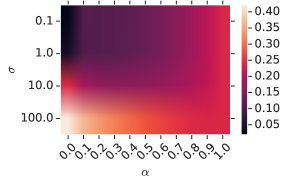
where $\Psi(z)\stackrel{{\scriptstyle.}}{{=}}(1+e^{-z})^{-1}$ is the sigmoid, $\alpha\in[0,1]$, $\sigma>0$, and and $\epsilon\sim\mathscr{N}(0,1)$ comprises independent Gaussian noise. Increasing $\alpha$ induces a bias in the teacher’s estimate of $p^{*}(x)$, while increasing $\sigma$ induces a variance in the teacher over fresh draws. Combined, these induce the teacher’s mean squared error (MSE) $\underset{}{\mathbb{E}}\left[\|p^{*}({x})-{p}^{\mathrm{t}}({x})\|_{2}^{2}\right]$, which by Proposition 3 bounds the gap between the population and distilled empirical risk.

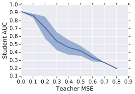
For each such teacher, we compute its MSE, as well as the test set AUC of the corresponding distilled student. Figure 5 shows the relationship between the the teacher’s MSE and the student’s AUC. In line with the theory, more accurate estimates of $p^{*}$ result in better students. Figure 6 also shows how the teacher’s MSE depends on the choice of $\sigma$ and $\alpha$, demonstrating that multiple such pairs can achieve a similar MSE. As before, we see that a teacher may trade-off bias for variance in order to achieve a low MSE.

Figure 5: Relationship between teacher’s MSE against true class-probability and student’s test set AUC. In keeping with the theory, teachers which better approximate $p^{*}$ yield better students.

Figure 6: Relationship between teacher’s bias and variance, and corresponding MSE against true class-probability. The teacher can achieve a given MSE through multiple possible bias-variance combinations.

B.2 Uncalibrated teachers may distill worse

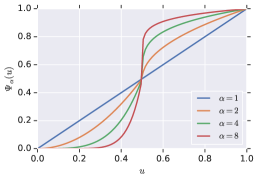
We now illustrate the importance of the teacher probabilities needing to be meaningful reflections of the true $p^{*}(x)$. We continue our exploration of the synthetic Gaussian problem, where $p^{*}$ takes on a sigmoid form. We now distort these probabilities as follows: for $\alpha\geq 1$, we construct

$$\bar{p}(x) =\Psi_{\alpha}(p^{*}(x))$$

$$\Psi_{\alpha}(u) =\begin{cases}\frac{1}{2}\cdot(2\cdot u)^{\alpha}&\text{ if }u\leq\frac{1}{2}\\ \frac{1}{2}+(2\cdot u-1)^{1/\alpha}&\text{ if }u\geq\frac{1}{2}.\end{cases}$$

The new class-probability function $\bar{p}(x)$ preserves the classification boundary $p^{*}(x)=\frac{1}{2}$, but squashes the probabilities themselves as $\alpha$ gets larger. We now consider using $\bar{p}(x)$ as teacher probabilities to distill to a student. This teacher has the same accuracy, but significantly worse calibration than the Bayes-teacher using $p^{*}(x)$.

Figure 7 confirms that as $\alpha$ increases, the effect of distilling on the student is harmed. This validates our claim that teacher accuracy is insufficient to judge whether distillation will be useful.

(a) As tuning parameter $\alpha$ is increased, the teacher probabilities $\bar{p}(x)=\Psi_{\alpha}(p^{*}(x))$ increasingly deviate from the Bayes probabilities $p^{*}(x)$.

(b) As tuning parameter $\alpha$ is increased — so that the teacher probabilities are increasingly uncalibrated — the student AUC becomes progressively worse.

Figure 7: Effect of distorting the Bayes probabilities $p^{*}(x)$ so as to preserve the classification decision boundary ($p^{*}(x)=\frac{1}{2}$), but degrade the calibration of the scores.

References

- Anil et al. (2018) Rohan Anil, Gabriel Pereyra, Alexandre Passos, Robert Ormandi, George E. Dahl, and Geoffrey E. Hinton. Large scale distributed neural network training through online distillation. In International Conference on Learning Representations, 2018. URL https://openreview.net/forum?id=rkr1UDeC-.
- Ba and Caruana (2014) Jimmy Ba and Rich Caruana. Do deep nets really need to be deep? In Z. Ghahramani, M. Welling, C. Cortes, N. D. Lawrence, and K. Q. Weinberger, editors, Advances in Neural Information Processing Systems 27, pages 2654–2662. Curran Associates, Inc., 2014.
- Bennett (1962) George Bennett. Probability inequalities for the sum of independent random variables. Journal of the American Statistical Association, 57(297):33–45, 1962.
- Bhatia et al. (2015) Kush Bhatia, Himanshu Jain, Purushottam Kar, Manik Varma, and Prateek Jain. Sparse local embeddings for extreme multi-label classification. In Advances in Neural Information Processing Systems, pages 730–738, 2015.
- Breiman and Shang (1996) Leo Breiman and Nong Shang. Born again trees. https://pdfs.semanticscholar.org/b6ba/5374ed8e09845996626bc62cc6d938e83fee.pdf, 1996.
- Bruch (2019) Sebastian Bruch. An alternative cross entropy loss for learning-to-rank. CoRR, abs/1911.09798, 2019.
- Bruch et al. (2019) Sebastian Bruch, Xuanhui Wang, Michael Bendersky, and Marc Najork. An analysis of the softmax cross entropy loss for learning-to-rank with binary relevance. In Proceedings of the 2019 ACM SIGIR International Conference on Theory of Information Retrieval, ICTIR ’19, page 75–78, New York, NY, USA, 2019. Association for Computing Machinery. ISBN 9781450368810.
- Bucilǎ et al. (2006) Cristian Bucilǎ, Rich Caruana, and Alexandru Niculescu-Mizil. Model compression. In Proceedings of the 12th ACM SIGKDD International Conference on Knowledge Discovery and Data Mining, KDD ’06, pages 535–541, New York, NY, USA, 2006. ACM.
- Buja et al. (2005) Andreas Buja, Werner Stuetzle, and Yi Shen. Loss functions for binary class probability estimation and classification: Structure and applications. Technical report, UPenn, 2005.
- Cao et al. (2019) Kaidi Cao, Colin Wei, Adrien Gaidon, Nikos Aréchiga, and Tengyu Ma. Learning imbalanced datasets with label-distribution-aware margin loss. In Advances in Neural Information Processing Systems 32: Annual Conference on Neural Information Processing Systems 2019, NeurIPS 2019, 8-14 December 2019, Vancouver, BC, Canada, pages 1565–1576, 2019.
- Celik et al. (2017) Z. B. Celik, D. Lopez-Paz, and P. McDaniel. Patient-driven privacy control through generalized distillation. In 2017 IEEE Symposium on Privacy-Aware Computing (PAC), pages 1–12, Aug 2017.
- Cohen et al. (1999) William W. Cohen, Robert E. Schapire, and Yoram Singer. Learning to order things. J. Artif. Intell. Res., 10:243–270, 1999.
- Crammer and Singer (2002) Koby Crammer and Yoram Singer. On the algorithmic implementation of multiclass kernel-based vector machines. J. Mach. Learn. Res., 2:265–292, March 2002. ISSN 1532-4435.
- Craven and Shavlik (1995) Mark W. Craven and Jude W. Shavlik. Extracting tree-structured representations of trained networks. In Proceedings of the 8th International Conference on Neural Information Processing Systems, NIPS’95, pages 24–30, Cambridge, MA, USA, 1995. MIT Press.
- Czarnecki et al. (2017) Wojciech M. Czarnecki, Simon Osindero, Max Jaderberg, Grzegorz Swirszcz, and Razvan Pascanu. Sobolev training for neural networks. In I. Guyon, U. V. Luxburg, S. Bengio, H. Wallach, R. Fergus, S. Vishwanathan, and R. Garnett, editors, Advances in Neural Information Processing Systems 30, pages 4278–4287. Curran Associates, Inc., 2017.
- Dekel et al. (2003) Ofer Dekel, Christopher D. Manning, and Yoram Singer. Log-linear models for label ranking. In Advances in Neural Information Processing Systems 16, pages 497–504, 2003.
- Dong et al. (2019) Bin Dong, Jikai Hou, Yiping Lu, and Zhihua Zhang. Distillation early stopping? harvesting dark knowledge utilizing anisotropic information retrieval for overparameterized neural network, 2019.
- Foster et al. (2019) Dylan J Foster, Spencer Greenberg, Satyen Kale, Haipeng Luo, Mehryar Mohri, and Karthik Sridharan. Hypothesis set stability and generalization. In Advances in Neural Information Processing Systems 32, pages 6726–6736. Curran Associates, Inc., 2019.
- Furlanello et al. (2018) Tommaso Furlanello, Zachary Chase Lipton, Michael Tschannen, Laurent Itti, and Anima Anandkumar. Born-again neural networks. In Proceedings of the 35th International Conference on Machine Learning, ICML 2018, Stockholmsmässan, Stockholm, Sweden, July 10-15, 2018, pages 1602–1611, 2018.
- Fürnkranz et al. (2008) Johannes Fürnkranz, Eyke Hüllermeier, Eneldo Loza Mencía, and Klaus Brinker. Multilabel classification via calibrated label ranking. Machine Learning, 73(2):133–153, 2008.
- Gotmare et al. (2019) Akhilesh Gotmare, Nitish Shirish Keskar, Caiming Xiong, and Richard Socher. A closer look at deep learning heuristics: Learning rate restarts, warmup and distillation. In International Conference on Learning Representations, 2019.
- Guo et al. (2017) Chuan Guo, Geoff Pleiss, Yu Sun, and Kilian Q. Weinberger. On calibration of modern neural networks. In Proceedings of the 34th International Conference on Machine Learning, ICML 2017, Sydney, NSW, Australia, 6-11 August 2017, pages 1321–1330, 2017.
- Hinton et al. (2015) Geoffrey E. Hinton, Oriol Vinyals, and Jeffrey Dean. Distilling the knowledge in a neural network. CoRR, abs/1503.02531, 2015.
- Jain et al. (2019) Himanshu Jain, Venkatesh Balasubramanian, Bhanu Chunduri, and Manik Varma. Slice: Scalable linear extreme classifiers trained on 100 million labels for related searches. In Proceedings of the Twelfth ACM International Conference on Web Search and Data Mining, WSDM ’19, pages 528–536, New York, NY, USA, 2019. ACM.
- Khan et al. (2019) S. Khan, M. Hayat, S. W. Zamir, J. Shen, and L. Shao. Striking the right balance with uncertainty. In 2019 IEEE/CVF Conference on Computer Vision and Pattern Recognition (CVPR), pages 103–112, 2019.
- Lapin et al. (2018) M. Lapin, M. Hein, and B. Schiele. Analysis and optimization of loss functions for multiclass, top-k, and multilabel classification. IEEE Transactions on Pattern Analysis and Machine Intelligence, 40(7):1533–1554, July 2018.
- Li and Hoiem (2018) Z. Li and D. Hoiem. Learning without forgetting. IEEE Transactions on Pattern Analysis and Machine Intelligence, 40(12):2935–2947, Dec 2018. ISSN 1939-3539.
- Li et al. (2019) Zeju Li, Konstantinos Kamnitsas, and Ben Glocker. Overfitting of neural nets under class imbalance: Analysis and improvements for segmentation. In Dinggang Shen, Tianming Liu, Terry M. Peters, Lawrence H. Staib, Caroline Essert, Sean Zhou, Pew-Thian Yap, and Ali Khan, editors, Medical Image Computing and Computer Assisted Intervention – MICCAI 2019, pages 402–410, Cham, 2019. Springer International Publishing.
- Liu et al. (2016) Weiyang Liu, Yandong Wen, Zhiding Yu, and Meng Yang. Large-margin softmax loss for convolutional neural networks. In Proceedings of the 33rd International Conference on International Conference on Machine Learning - Volume 48, ICML’16, page 507–516. JMLR.org, 2016.
- Liu et al. (2017) Weiyang Liu, Yandong Wen, Zhiding Yu, Ming Li, Bhiksha Raj, and Le Song. Sphereface: Deep hypersphere embedding for face recognition. In 2017 IEEE Conference on Computer Vision and Pattern Recognition, CVPR 2017, Honolulu, HI, USA, July 21-26, 2017, pages 6738–6746, 2017.
- Liu et al. (2019) Yu Liu, Xuhui Jia, Mingxing Tan, Raviteja Vemulapalli, Yukun Zhu, Bradley Green, and Xiaogang Wang. Search to distill: Pearls are everywhere but not the eyes, 2019.
- Lopez-Paz et al. (2016) D. Lopez-Paz, B. Schölkopf, L. Bottou, and V. Vapnik. Unifying distillation and privileged information. In International Conference on Learning Representations (ICLR), November 2016.
- Maurer and Pontil (2009) Andreas Maurer and Massimiliano Pontil. Empirical bernstein bounds and sample-variance penalization. In COLT 2009 - The 22nd Conference on Learning Theory, Montreal, Quebec, Canada, June 18-21, 2009, 2009.
- McAuley and Leskovec (2013) Julian McAuley and Jure Leskovec. Hidden factors and hidden topics: Understanding rating dimensions with review text. In Proceedings of the 7th ACM Conference on Recommender Systems, RecSys ’13, page 165–172, New York, NY, USA, 2013. Association for Computing Machinery. ISBN 9781450324090.
- Mobahi et al. (2020) Hossein Mobahi, Mehrdad Farajtabar, and Peter L. Bartlett. Self-distillation amplifies regularization in hilbert space, 2020.
- Müller et al. (2019) Rafael Müller, Simon Kornblith, and Geoffrey E. Hinton. When does label smoothing help? In Advances in Neural Information Processing Systems 32: Annual Conference on Neural Information Processing Systems 2019, NeurIPS 2019, 8-14 December 2019, Vancouver, BC, Canada, pages 4696–4705, 2019.
- Nayak et al. (2019) Gaurav Kumar Nayak, Konda Reddy Mopuri, Vaisakh Shaj, Venkatesh Babu Radhakrishnan, and Anirban Chakraborty. Zero-shot knowledge distillation in deep networks. In Proceedings of the 36th International Conference on Machine Learning, ICML 2019, 9-15 June 2019, Long Beach, California, USA, pages 4743–4751, 2019.
- Papernot et al. (2016) Nicolas Papernot, Patrick D. McDaniel, Xi Wu, Somesh Jha, and Ananthram Swami. Distillation as a defense to adversarial perturbations against deep neural networks. In IEEE Symposium on Security and Privacy, SP 2016, San Jose, CA, USA, May 22-26, 2016, pages 582–597, 2016.
- Phuong and Lampert (2019) Mary Phuong and Christoph Lampert. Towards understanding knowledge distillation. In Kamalika Chaudhuri and Ruslan Salakhutdinov, editors, Proceedings of the 36th International Conference on Machine Learning, volume 97 of Proceedings of Machine Learning Research, pages 5142–5151, Long Beach, California, USA, 09–15 Jun 2019. PMLR.
- Radosavovic et al. (2018) Ilija Radosavovic, Piotr Dollár, Ross B. Girshick, Georgia Gkioxari, and Kaiming He. Data distillation: Towards omni-supervised learning. In 2018 IEEE Conference on Computer Vision and Pattern Recognition, CVPR 2018, Salt Lake City, UT, USA, June 18-22, 2018, pages 4119–4128, 2018.
- Reddi et al. (2019) Sashank J. Reddi, Satyen Kale, Felix Yu, Daniel Holtmann-Rice, Jiecao Chen, and Sanjiv Kumar. Stochastic negative mining for learning with large output spaces. In Proceedings of Machine Learning Research, volume 89 of Proceedings of Machine Learning Research, pages 1940–1949. PMLR, 16–18 Apr 2019.
- Rothfuss et al. (2019) Jonas Rothfuss, Fabio Ferreira, Simon Boehm, Simon Walther, Maxim Ulrich, Tamim Asfour, and Andreas Krause. Noise regularization for conditional density estimation, 2019.
- Rudin (2009) Cynthia Rudin. The P-Norm Push: A simple convex ranking algorithm that concentrates at the top of the list. Journal of Machine Learning Research, 10:2233–2271, Oct 2009.
- Rusu et al. (2016) Andrei A. Rusu, Sergio Gomez Colmenarejo, Çaglar Gülçehre, Guillaume Desjardins, James Kirkpatrick, Razvan Pascanu, Volodymyr Mnih, Koray Kavukcuoglu, and Raia Hadsell. Policy distillation. In 4th International Conference on Learning Representations, ICLR 2016, San Juan, Puerto Rico, May 2-4, 2016, Conference Track Proceedings, 2016.
- Savage (1971) Leonard J. Savage. Elicitation of personal probabilities and expectations. Journal of the American Statistical Association, 66(336):783–801, 1971. ISSN 01621459.
- Schervish (1989) Mark J. Schervish. A general method for comparing probability assessors. Ann. Statist., 17(4):1856–1879, 12 1989.
- Szegedy et al. (2016) Christian Szegedy, Vincent Vanhoucke, Sergey Ioffe, Jonathon Shlens, and Zbigniew Wojna. Rethinking the inception architecture for computer vision. In 2016 IEEE Conference on Computer Vision and Pattern Recognition, CVPR 2016, Las Vegas, NV, USA, June 27-30, 2016, pages 2818–2826, 2016.
- Tang and Wang (2018) Jiaxi Tang and Ke Wang. Ranking distillation: Learning compact ranking models with high performance for recommender system. In Proceedings of the 24th ACM SIGKDD International Conference on Knowledge Discovery & Data Mining, KDD ’18, page 2289–2298, New York, NY, USA, 2018. Association for Computing Machinery. ISBN 9781450355520.
- Tang et al. (2020) Jiaxi Tang, Rakesh Shivanna, Zhe Zhao, Dong Lin, Anima Singh, Ed H. Chi, and Sagar Jain. Understanding and improving knowledge distillation. CoRR, abs/2002.03532, 2020. URL https://arxiv.org/abs/2002.03532.
- Tang et al. (2016) Zhiyuan Tang, Dong Wang, and Zhiyong Zhang. Recurrent neural network training with dark knowledge transfer. In 2016 IEEE International Conference on Acoustics, Speech and Signal Processing, ICASSP 2016, Shanghai, China, March 20-25, 2016, pages 5900–5904, 2016.
- Usunier et al. (2009) Nicolas Usunier, David Buffoni, and Patrick Gallinari. Ranking with ordered weighted pairwise classification. In Proceedings of the 26th Annual International Conference on Machine Learning, ICML ’09, pages 1057–1064, New York, NY, USA, 2009. ACM.
- Vembu and Gärtner (2011) Shankar Vembu and Thomas Gärtner. Label Ranking Algorithms: A Survey, pages 45–64. Springer Berlin Heidelberg, Berlin, Heidelberg, 2011.
- Wang et al. (2018) F. Wang, J. Cheng, W. Liu, and H. Liu. Additive margin softmax for face verification. IEEE Signal Processing Letters, 25(7):926–930, 2018.
- Xie et al. (2019) Qizhe Xie, Eduard Hovy, Minh-Thang Luong, and Quoc V. Le. Self-training with noisy student improves imagenet classification, 2019.
- Xue et al. (2013) Jian Xue, Jinyu Li, and Yifan Gong. Restructuring of deep neural network acoustic models with singular value decomposition. In Interspeech, January 2013.
- Yang et al. (2019) Chenglin Yang, Lingxi Xie, Siyuan Qiao, and Alan L. Yuille. Training deep neural networks in generations: A more tolerant teacher educates better students. In The Thirty-Third AAAI Conference on Artificial Intelligence, AAAI 2019, pages 5628–5635, 2019.
- Yim et al. (2017) J. Yim, D. Joo, J. Bae, and J. Kim. A gift from knowledge distillation: Fast optimization, network minimization and transfer learning. In 2017 IEEE Conference on Computer Vision and Pattern Recognition (CVPR), pages 7130–7138, July 2017.
- Yun et al. (2014) Hyokun Yun, Parameswaran Raman, and S. V. N. Vishwanathan. Ranking via robust binary classification. In Advances in Neural Information Processing Systems 27: Annual Conference on Neural Information Processing Systems 2014, December 8-13 2014, Montreal, Quebec, Canada, pages 2582–2590, 2014.
- Zhang et al. (2018) Hongyi Zhang, Moustapha Cisse, Yann N. Dauphin, and David Lopez-Paz. mixup: Beyond empirical risk minimization. In International Conference on Learning Representations, 2018.