MDPs with Unawareness in Robotics

Abstract

We formalize decision-making problems in robotics and automated control using continuous MDPs and actions that take place over continuous time intervals. We then approximate the continuous MDP using finer and finer discretizations. Doing this results in a family of systems, each of which has an extremely large action space, although only a few actions are “interesting”. We can view the decision maker as being unaware of which actions are “interesting”. We can model this using MDPUs, MDPs with unawareness, where the action space is much smaller. As we show, MDPUs can be used as a general framework for learning tasks in robotic problems. We prove results on the difficulty of learning a near-optimal policy in an an MDPU for a continuous task. We apply these ideas to the problem of having a humanoid robot learn on its own how to walk.

1 INTRODUCTION

Markov decision processes (MDPs) are widely used for modeling decision making problems in robotics and automated control. Traditional MDPs assume that the decision maker (DM) knows all states and actions. However, in many robotics applications, the space of states and actions is continuous. To find appropriate policies, we typically discretize both states and actions. However, we do not know in advance what level of discretization is good enough for getting a good policy. Moreover, in the discretized space, the set of actions is huge. However, relatively few of the actions are “interesting”. For example, when flying a robotic helicopter, only a small set of actions lead to useful flying techniques; an autonomous helicopter must learn these techniques. Similarly, a humanoid robot needs to learn various maneuvers (e.g., walking or running) that enable it to move around, but the space of potential actions that it must search to find a successful gait is huge, while most actions result in the robot losing control and falling down.

Halpern, Rong, and Saxena [?] (HRS from now on) defined MDPs with unawareness (MDPUs), where a decision-maker (DM) can be unaware of the actions in an MDP. In the robotics applications in which we are interested, we can think of the DM (e.g., a humanoid robot) as being unaware of which actions are the useful actions, and thus can model what is going on using an MDPU.

In this paper, we apply MDPUs to continuous problems. We model such problems using continuous MDPs, where actions are performed over a continuous duration of time. Although many problems fit naturally in our continuous MDP framework, and there has been a great deal of work on continuous-time MDPs, our approach seems new, and of independent interest. (See the discussion in Section 5.) It is hard to find near-optimal policies in continuous MDPs. A standard approach is to use discretization. We use discretization as well, but our discrete models are MDPUs, rather than MDPs, which allows us both to use relatively few actions (the “interesting actions”), while taking into account the possibility of there being interesting actions that the DM has not yet discovered. We would like to find a discretization level for which the optimal policy in the MDP underlying the approximating MDPU provides a good approximation to the optimal policy in the continuous MDP that accurately describes the problem, and then find a near-optimal policy in that discretized MDPU.

HRS gave a complete characterization of when it is possible to learn to play near-optimally in an MDPU, extending earlier work [Brafman and Tennenholtz 2002, Kearns and Singh 2002] showing that it is always possible to learn to play near-optimally in an MDP. We extend and generalize these results so as to apply them to the continuous problems of interest to us. We characterize when brute-force exploration can be used to find a near-optimal policy in our setting, and show that a variant of the URMAX algorithm presented by HRS can find a near-optimal policy. We also characterize the complexity of learning to play near-optimally in continuous problems, when more “guided” exploration is used. Finally, we discuss how MDPUs can be used to solve a real robotic problem: to enable a humanoid robot to learn walking on its own. In our experiment, the robot learned various gaits at multiple discretization levels, including both forward and backward gaits; both efficient and inefficient gaits; and both gaits that resemble human walking, and those that do not.

2 MDPU: A REVIEW

In this section, we review the definition of MDPU and the results of HRS show that is possible for a DM to learn to play near-optimally.

In the standard MDP model, we have a set of actions, and states representing the complete set of actions and states that are available to the Decision Maker (DM). Describing a situation by a standard MDP misses out on some important features. In general, an agent may not be aware of all the actions that can be performed. For example, an agent playing a video game may not be aware of all actions that can be performed in a given state. Our model is compatible with a number of interpretations of unawareness. In the robotics setting, we take a particular concrete interpretation. Here, the number of actions is typically extremely large, but only a few of these actions are actually useful. For example, although an autonomous helicopter can have a huge number of actions, only a few are useful for flying the helicopter, whereas the rest simply result in a crash. We can abstract what is going on by defining a set of “useful actions”. The DM may initial be unaware of many or even most of the useful actions. A DM may become aware of a useful action (and thus, can safely perform it) by performing a special action called the explore action, denoted $a_{0}$. Playing the explore action results in the DM learning about new actions with some probability.

We thus take an MDPU to be a tuple $M=(S,A,A_{0},g,a_{0},g_{0},P,D,R)$, where the tuple $(S,A,g,P,R)$ is a standard MDP—that is, $S$ is a set of states, $A$ is a set of actions, $g(s)$ is the set of actions available at state $s$, for each tuple $(s,s^{\prime},a)\in S\times S\times A$, $P(s,s^{\prime},a)$ gives the probability of making a transition from $s$ to $s^{\prime}$ if action $a$ is performed, and $R(s,s^{\prime},a)$ gives the reward earned by the DM if this transition is taken; $A_{0}\subseteq A$ is the set of actions that the DM initially knows to be useful; $a_{0}$ is the special explore action; $g(s)\subseteq A$ is the set of actions that can be performed at state $s$; $g_{0}(s)\subseteq A_{0}\cap g(s)$ is the set of actions that the DM is aware of at state $s$; finally, $D$ is the discovery probability function. $D(j,t,s)$ is the probability of discovering a useful action given that there are $j$ useful actions to be discovered at state $s$, and $a_{0}$ has already been played $t-1$ times without discovering a useful action. Intuitively, $D$ describes how quickly the DM can discover a useful action. We assume that $D(j,t,s)$ is non-decreasing as a function of $j$: the more useful actions there are to be found, the easier we can find one. How $D(j,t,s)$ varies with $t$ depends on the problem. In the sequel, we assume for ease of exposition that $D(j,t,s)$ is independent of $s$, so we write $D(j,t)$ rather than $D(j,t,s)$. $M^{\prime}=(S,A,P,R)$ is called the MDP underlying $M$.

Kearns and Singh [?] and Brafman and Tennenholtz [?] have studied the problem of learning how to play near-optimally in an MDP. Roughly speaking, to play near-optimally means that, for all $\epsilon>0$ and $\delta>0$, we can find a policy that obtains expected reward $\epsilon$-close to that of the optimal policy with probability at least $1-\delta$. HRS completely characterize the difficulty of learning to play near-optimally in an MDPU. We briefly review the relevant results here. Despite initially being unaware of some useful actions, we want the DM to learn a policy that is near-optimal in the underlying MDP. HRS showed that whether a DM can learn to play optimally and how long it takes depend on the value of $D(1,t)$—the probability of discovering a new action given that there is a new action to discover and the DM has tried $t-1$ times in the past to discover a new action.

The first result characterizes when it is impossible to learn to play near-optimally. It turns out that the result holds even if the DM has quite a bit of information, as made precise by the following definition.

Definition 2.1

: Define a DM to be quite knowledgeable if (in addition to $S$, $D$) she knows $|A|$, the transition function $P_{0}$, the reward function $R_{0}$ for states in $S$ and actions in $A_{0}$, and $R_{\max}$.

Another relevant concept that we need to define is the mixing time. A policy $\pi$ may take a long time to reach its expected payoff. For example, if getting a high reward involves reaching a particular state $s^{*}$, and the probability of reaching $s^{*}$ from some state $s$ is low, then the time to get the high reward will be high. To deal with this, Kearns and Singh [?] argue that the running time of a learning algorithm should be compared to the time that an algorithm with full information takes to get a comparable reward.

Definition 2.2

: Define the $\epsilon$-return mixing time of policy $\pi$ to be the smallest value of $T$ such that $\pi$ guarantees an expected payoff of at least $U(\pi)-\epsilon$; that is, it is the least $T$ such that $U(s,\pi,t)\geq U(\pi)-\epsilon$ for all states $s$ and times $t\geq T$.

The following theorem shows that if the discovery probability is sufficiently low, where “sufficiently low” means $D(1,t)<1$ for all $t$ and $\sum_{t=1}^{\infty}D(1,t)<\infty$, then the DM cannot learn to play near-optimally. We define $\Psi(T)=\sum_{t=1}^{T}D(1,t)$.

Theorem 2.3

: If $D(1,t)<1$ for all $t$ and $\Psi(\infty)<\infty$, then there exists a constant $c$ such that no algorithm can obtain a reward that is guaranteed to be within $c$ of optimal for an MDPU $M=(S,A,A_{0},G,a_{o}g_{0},P,D,R)$, even if $S$, $|A|$, and a bound on the optimal reward are known.

Theorem 2.3 says that when $\Psi(\infty)<\infty$, it is impossible for the DM to learn an optimal policy. On the other hand, if $\Psi(\infty)=\infty$, then it is possible to learn to play near-optimally. HRS present an algorithm called URMAX, a variant of the RMAX algorithm [Brafman and Tennenholtz 2002], that learns near-optimal play.

Theorem 2.4

: If $\Psi(\infty)=\infty$, then the URMAX algorithm computes a near-optimal policy.

In fact, we can say even more. If $\Psi(\infty)=\infty$, then the efficiency of the best algorithm for determining near-optimal play depends on how quickly $\Psi(\infty)$ diverges. HRS characterize the running time of URMAX in terms of the function $\Psi$, and give lower bounds on the time required to learn near-optimally in terms of $\Psi$. These results show that URMAX learns to play near-optimally almost as quickly as possible. Specifically, it learns a policy with an expected reward $\epsilon$-close to the optimal reward with probability $1-\delta$ in time polynomial in $|S|$, $|A|$, $1/\epsilon$, $1/\delta$, a bound $R_{\max}$ on the optimal reward, the $\epsilon$-return mixing time, and the smallest $T$ such that $\Psi(T)\geq\ln(4N/\delta)$, whenever it is possible to do so. The polynomial-time results are summarized in the next result.

Theorem 2.5

: It is possible to learn to play near-optimally in polynomial time iff there exist constants $m_{1}$ and $m_{2}$ such that $\Psi(T)\geq m_{1}\ln(T)+m_{2}$ for all $T>0$. Moreover, if it is possible to learn to play near-optimally in polynomial time, URMAX does so.

3 ANALYZING ROBOTIC PROBLEMS AS MDPUS

As we said in the introduction, we apply the MDPU framework to robotic problems such as having a humanoid robot learn to walk. For such problems, we typically have a continuous space of states and actions, where actions take place in continuous time, and actions have a nontrivial duration.

Suppose that the original continuous problem can be characterized by a continuous MDP $M_{\infty}$ (defined formally below). We would like to find a “good” discretization $M$ of $M_{\infty}$. “Good” in this setting means that an optimal policy for $M$ is $\epsilon$-optimal for $M_{\infty}$, for some appropriate $\epsilon$. Clearly the level of discretization matters. Too coarse a discretization results in an MDP whose optimal policy is not $\epsilon$-optimal for $M_{\infty}$; on the other hand, too fine a discretization results in the problem size becoming unmanageably large. For example, in order to turn a car on a smooth curve (without drifting), the optimal policy is to slowly turn the steering wheel to the left and back, in which the action varies smoothly over time. This can be simulated using a relatively coarse discretization of time. However, in order to make a sharp turn using advanced driving techniques like drifting, the steering wheel needs to be turned at precise points in time, or else the car will go into an uncontrollable spin. In this case, a fine discretization in time is needed.

Unfortunately, it is often not clear what discretization level to use in a specific problem. Part of the DM’s problem is to find the “right” level of discretization. Thus, we describe the problem in terms of a continuous MDP $M_{\infty}$ and a sequence $((M_{1},M_{1}^{\prime}),(M_{2},M_{2}^{\prime}),\ldots)$, where $M_{i}$ is an MDPU with underlying MDP $M_{i}^{\prime}$, for $i=1,2,\ldots$. Intuitively, $(M_{1}^{\prime},M_{2}^{\prime},M_{3}^{\prime},\ldots)$ represents a sequence of finer and finer approximations to $M_{\infty}$.

Continuous Time MDP with Continuous Actions over Time: To make this precise, we start by defining our model of continuous MDPs. Let $M_{\infty}=(S_{\infty},A_{\infty},g_{\infty},P_{\infty},R_{\infty})$. $S_{\infty}$ is a continuous state space, which we identify with a compact subset of $\mbox{$I\!\!R$}^{n}$ for some integer $n>0$; that is, each state can be represented by a vector $(s_{1},\cdots,s_{n})$ of real numbers. For example, for a humanoid robot, the state space can be described by a vector which includes the robot’s $(x,y,z)$ position, and the current positions of its movable joints.

Actions: Describing $A_{\infty}$ requires a little care. We assume that there is an underlying set of basic actions $A_{B}$, which can be identified with a compact subset of $\mbox{$I\!\!R$}^{m}$ for some $m>0$; that is, each basic action can be represented by a vector $(a_{1},\cdots,a_{m})$ of real numbers. For example, for a humanoid robot, the basic actions can be characterized by a tuple that contains the targeted positions for its movable joints. However, we do not take $A_{\infty}$ to consist of basic actions. Rather, an action is a path of basic actions over time. Formally, an action in $A_{\infty}$ is a piecewise continuous function from a domain of the form $(0,t]$ for some $t>0$ to basic actions. Thus, there exist time points $t_{0}<t_{1}<\ldots<t_{k}$ with $t_{0}=0$ and $t_{k}=t$ such that $a$ is continuous in the interval $(t_{j},t_{j+1}]$ for all $j<k$. The number $t$ is the length of the action $a$, denoted $|a|$. We use left-open right-closed intervals here; we think of the action in the interval $(t_{j},t_{j+1}]$ as describing what the DM does right after time $t_{j}$ until time $t_{j+1}$. By analogy with the finite case, $g_{\infty}(s)$ is the set of actions in $A_{\infty}$ available at $s$.

Reward and Transition Functions: We now define $R_{\infty}$ and $P_{\infty}$, the reward and transition functions. In a discrete MDP, the transition function $P$ and reward function $R$ take as arguments a pair of states and an action. Thus, for example, $P(s_{1},s_{2},a)$ is the probability of transitioning from $s_{1}$ to $s_{2}$ using action $a$, and $R(s_{1},s_{2},a)$ is the reward the agent gets if a transition from $s_{1}$ to $s_{2}$ is taken using action $a$. In our setting, what matters is the path taken by a transition according to $a$. Thus, we take the arguments to $P_{\infty}$ and $R_{\infty}$ to be tuples of the form $(s_{1},s_{c},a)$, where $s_{1}$ is a state, $a$ is an action in $A_{\infty}$ of length $t$, and $s_{c}$ is a piecewise continuous function from $(0,t]$ to $S_{\infty}$. Intuitively, $s_{c}$ describes a possible path of states that the DM goes through when performing action $a$, such that before $a$ starts, the DM was at $s_{1}$. Note that we do not require that $\lim_{t\rightarrow 0^{+}}s_{c}(t)=s_{1}$. Intuitively, this means that there can be a discrete change in state at the beginning of an interval. This allows us to capture the types of discrete changes considered in semi-MDPs [Puterman 1994].

We think of $R_{\infty}(s_{1},s_{c},a)$ as the reward for transitioning from $s_{1}$ according to state path $s_{c}$ via action $a$. We assume that $R_{\infty}$ is bounded: specifically, there exists a constant $c$ such that $R_{\infty}(s_{1},s_{c},a)<c\cdot|a|$. For state $s_{1}\in S_{\infty}$ and action $a\in A_{\infty}$, we take $P_{\infty}(s_{1},\cdot,a)$ to be a probability density function over state paths of length $|a|$ starting at $s_{1}$. $P_{\infty}$ is not defined for transitions starting at terminal states.

We require $R_{\infty}$ and $P_{\infty}$ to be continuous functions, so that if $(s_{i},s_{c}^{i},a_{i})$ approaches $(s,s_{c},a)$ (where all the state sequences and actions have the same length $t$), then $R_{\infty}(s_{i},s_{c}^{i},a_{i})$ approaches $R_{\infty}(s,s_{c},a)$ and $P_{\infty}(s_{i},s_{c}^{i},a_{i})$ approaches $P_{\infty}(s,s_{c},a)$. To make the notion of “approaches” precise, we need to consider the distance between state paths and the distance between actions. Since we have identified both states (resp., basic actions) with subsets of $\mbox{$I\!\!R$}^{n}$ (resp., $\mbox{$I\!\!R$}^{m}$), this is straightforward. For definiteness, we define the distance between two vectors in $\mbox{$I\!\!R$}^{n}$ using the $L_{1}$ norm, so that $d(\vec{p},\vec{q})=\sum_{1}^{n}|p_{i}-q_{i}|$. For actions $a$ and $a^{\prime}$ in $A_{\infty}$ of the same length, define $d(a,a^{\prime})=\int_{t=0}^{|a|}d(a(t),a^{\prime}(t))dt$. For state paths $s_{c}$ and $s_{c}^{\prime}$ of the same length, define $d(s_{c},s_{c}^{\prime})=\int_{t=0}^{|s_{c}|}d(s_{c}(t),s_{c}^{\prime}(t))dt$. Finally, define $d((s_{c},a),(s_{c}^{\prime},a^{\prime}))=d(s_{c},s_{c}^{\prime})+d(a,a^{\prime})$. This definition of distance allows us to formalize the notion of continuity for $R_{\infty}$ and $P_{\infty}$. The key point of the continuity assumption is that it allows us to work with discretizations, knowing that they really do approximate the continuous MDP.

Constraints on Actions: We typically do not want to take $A_{\infty}$ to consist of all possible piecewise continuous functions. For one thing, some hardware and software restrictions will make certain functions infeasible. For example, turning a steering wheel back and forth $10^{20}$ times in one second can certainly be described by a continuous function, but is obviously infeasible in practice. But we may want to impose further constraints on $A_{\infty}$ and $g_{\infty}(s)$.

In the discussion above, we did not place any constraints on the length of actions. When we analyze problems of interest, there is typically an upper bound on the length of actions of interest. For example, when playing table tennis using a robotic arm, the basic actions can be viewed as tuples, describing the direction of movement of the racket, the rotation of the racket, and the force being applied to the racket; actions are intuitively all possible control sequences of racket movements that are feasible according to the robot’s hardware and software constraints; this includes slight movements of the racket, strokes, and prefixes of strokes. An example of a piecewise continuous action here would be to move the racket forward with a fixed force for some amount of time, and then to suddenly stop applying the force when the racket is close to the ball. We can bound the length of actions of interest to the time that a ball can be in the air between consecutive turns.

Awareness: Even with the constraints discussed above, $A_{\infty}$ is typically extremely large. Of course, not all actions in $A_{\infty}$ are “useful”. For instance, in the helicopter example, most actions would crash the helicopter. We thus consider potentially useful actions. (We sometimes call them just useful actions.) Informally, an action is potentially useful if it is not useless. A useless action is one that either destroys the robot, or leaves it in an uncontrollable state, or does not change the state. For example, when flying a helicopter, actions that lead to a crash are useless, as are actions that make the helicopter lose control. More formally, given a state $s$, the set of useful actions at state $s$ are the actions that transit to a different state in which the robot is neither destroyed nor uncontrollable. Note that an action that crashes the helicopter in one state may not cause a crash in a different state. For robotics applications, we say that a robot is aware of an action if it identifies that action as a potentially useful action, either because it has been preprogrammed with the action (we are implicitly assuming that the robot understands all actions with which it has been programmed) or it has simulated the action. For example, a humanoid robot that has been pre-programmed with only simple walking actions, and has never tried running or simulated running before, would be unaware of running actions. Let $\bar{A}_{\infty}$ denote the useful actions in $A_{\infty}$, and let $\bar{A}_{\infty 0}$ denote the useful actions that the robot is initially aware of. (These are usually the actions that the robot has been pre-programmed with.)

Discretization: We now consider the discretization of $M_{\infty}$. We assume that, for each discretization level $i$, $S_{\infty}$ is discretized into a finite state space $S_{i}$ and $A_{B}$ is discretized into a finite basic action space $A_{Bi}$, where $|S_{1}|\leq|S_{2}|\leq\ldots$ and $|A_{B1}|\leq|A_{B2}|\leq\ldots$. We further assume that, for all $i$, there exists $d_{i}>0$, with $d_{i}\rightarrow 0$, such that for all states $s\in S_{\infty}$ and basic actions $a_{B}\in A_{B}$, there exists a state $s^{\prime}\in S_{i}$ and a basic action $a_{B^{\prime}}\in A_{Bi}$ such that $d(s,s^{\prime})\leq d_{i}$, and $d(a_{B},a_{B}^{\prime})\leq d_{i}$. Thus, we are assuming that the discretizations can give closer and closer approximations to all states and basic actions. At level $i$, we also discretize time into time slices of length $t_{i}$, where $T\geq t_{1}>t_{2}>\ldots$.Thus, actions at discretization level $i$ are sequences of constant actions of length $t_{i}$, where a constant action is a constant function from $(0,t_{i}]$ to a single basic action. In other words, the action lengths at discretization level $i$ are multiples of $t_{i}$. Thus, at discretization level $i$, there are $\sum_{l=1}^{\left\lfloor T/t_{i}\right\rfloor}|A_{Bi}|^{l}$ possible actions. To see why, there are $|A_{Bi}|$ discrete actions at level $i$, and action lengths must be multiples of $t_{i}$. Thus, action lengths must have the form $lt_{i}$ for some $l\leq\lfloor T/t_{i}\rfloor$. There are $|A_{Bi}|^{l}$ actions of length $l\times t_{i}$ at level $i$, and thus $\sum_{l=1}^{\left\lfloor T/t_{i}\right\rfloor}|A_{Bi}|^{l}$ actions at level $i$. Let $A_{i}^{\prime}$ consist of this set of actions. (Note that some actions in $A_{i}^{\prime}$ may not be in $A_{\infty}$, since certain action sequences might be infeasible due to hardware and software constraints.) Let $A_{i}\subseteq A_{i}^{\prime}$ be the set of useful actions at level $i$.

Let $M_{i}$ be the MDPU where $S_{i}$ and $A_{i}$ are defined above; $A_{\infty 0}$ is the set of useful actions that the DM is initially aware of; $g(s)$ is the set of useful actions at state $s$; $g_{0}(s)$ is the set of useful actions that the DM is aware of at state $s$; and the reward function $R_{i}$ is just the restriction of $R_{\infty}$ to $A_{i}$ and $S_{i}$. For $s_{1}\in S_{i}$ and $a\in A_{i}$, we take $P_{i}(s_{1},\cdot,a)$ to be a probability distribution over $Q_{i}^{|a|}$, the set of state paths of length $|a|$ that are piecewise constant and each constant section has a length that is a multiple of $t_{i}$. For a state path $s_{c}\in Q_{i}^{|a|}$, let $P_{i}(s_{1},s_{c},a)$ be the normalized probability of traversing a state sequence that is within distance $d_{i}$ of state sequence $s_{c}$ when playing action $a$ starting from state $s_{1}$. Formally, $P_{i}(s_{1},s_{c},a)=(\int_{\{s_{c}^{\prime}:d(s_{c},s_{c}^{\prime})\leq d_{i}\}}dP_{\infty}(s_{1},\cdot,a))/c$, where $c=\sum_{s_{c}\in Q_{i}^{|a|}}\int_{\{s_{c}^{\prime}:d(s_{c},s_{c}^{\prime})\leq d_{i}\}}dP_{\infty}(s_{1},\cdot,a)$ is a normalization constant. Since the robot is not assumed to know all useful actions at any specific discretization level, it needs to explore for the useful actions it wasn’t aware of. Finally, given a specific exploration strategy, $D_{i}(j,t)$ describes the probability of discovering a new useful action at discretization level $i$, given that there are $j$ undiscovered useful actions at level $i$, and the robot has explored $t$ times without finding a useful action. We model exploration using $a_{0}$; every time the robot explores, it is playing $a_{0}$.

It remains to define the discretization of an action in $A_{0}$. In order to do this, for $a\in A_{\infty}$, define $a_{i}\in A_{i}$ to be a best approximation to $a$ in level $i$ if $|a_{i}|$ is the largest multiple of $t_{i}$ that is less than or equal to $|a|$, and $\int_{0}^{(|a_{i}|)}d(a(t),a_{i}(t))dt$ is minimal among actions $a^{\prime}\in A$ of length $|a_{i}|$. Intuitively, $a_{i}$ is an action in $A_{i}$ whose length is as close as possible to that of $a$ and, among actions of that length, is closest in distance to $a$. The action $a_{i}$ is not unique. For $a\in A_{0}$, define its discretization at level $i$ to be a best approximation to $a$ at that level. When there are several best approximations, we choose any one of them.

Policies: As usual, a policy $\pi$ in $M_{i}$ is a function from $S_{i}$ to $A_{i}$. We want to compute $U_{M_{i}}(s,\pi,t)$, the expected average reward over time $t$ of $\pi$ started in state $s\in S_{i}$. Let $a_{j}\in A_{i}$ and $s_{cj}$ be a state sequence in $Q_{i}^{|a_{j}|}$, for $j=0,\ldots,l$. Say that a sequence $((a_{0},s_{c0}),(a_{1},s_{c1}),\cdots,(a_{l},s_{cl}))$ is a path compatible with policy $\pi$ starting at $s$ if $\pi(s)=a_{0}$ and $\pi(s_{cj}(|a_{j}|))=a_{j+1}$ for all $0\leq j\leq l-1$. Let $I_{s,t}^{\pi}$ consist of all paths $((a_{0},s_{c0}),(a_{1},s_{c1}),\cdots,(a_{l},s_{cl}))$ starting at $s$ compatible with $\pi$ such that $\sum_{j=0}^{l}|a_{j}|\leq t<\sum_{j=0}^{l+1}|a_{j}|$, where $a_{l+1}=\pi(s_{cl}(|a_{l}|))$. Essentially, when computing $U_{M_{i}}(s,\pi,t)$, we consider the expected reward over all maximally long paths that have total length at most $t$. Thus, $U_{M_{i}}(s,\pi,t)=\sum_{p\in I^{\pi}_{s,t}}P^{*}_{i}(p)\frac{R^{*}_{i}(p)}{t}$, where, given a path $p=((a_{0},s_{c0}),(a_{1},s_{c1}),\cdots,(a_{l},s_{cl}))$, $P_{i}^{*}(p)=\Pi_{j=0}^{l}P_{i}(s_{cj}(0),s_{cj},a_{j})$, and $R_{i}^{*}(p)=\sum_{j=0}^{l}{R_{i}(s_{cj}(0),s_{cj},a_{j})}$.

Now that we have defined the average reward of a policy at discretization level $i$, we can define the average reward of a policy in $M_{\infty}$. Given a discretization level $i$, let $\pi_{i}$ be a projection of $\pi_{\infty}$ at level $i$, defined as follows: for each $s_{i}\in S_{i}$, define $\pi_{i}(s_{i})$ to be an action $a_{i}\in A_{i}$ such that $a_{i}$ is a best approximation to $\pi(s_{i})$ at level $i$, as defined above. As mentioned, there might be several best approximations; $a_{i}$ is not unique. Thus, the projection is not unique. Nevertheless, we define $U_{M_{\infty}}(s,\pi_{\infty},t)$ to be $\lim_{i\rightarrow\infty}U_{M_{i}}(s,\pi_{i},t)$, where $\pi_{i}$ is a projection of $\pi$ to discretization level $i$. The continuity of the transition and reward functions guarantees that the limit exists and is independent of the choice of projections.

We now consider how the URMAX algorithm of Section 2 can be applied to learn near-optimal policies. We use URMAX at each discretization level. Note that URMAX never terminates; however, it eventually learns to play near-optimally (although we may not know exactly when). The time it takes to learn to play near-optimally depends on the exploration strategy. The next theorem consider brute-force searching, where, at discretization level $i$, at each discretization level $i$, all actions in $A_{i}^{\prime}$ are exhaustively examined to find useful actions. (The proof of this and all other theorems can be found in the supplementary material.)

Theorem 3.1

: Using brute-force exploration, given $\alpha>0$ and $0<\delta<1$, we can find an $\alpha$-optimal policy in $M_{\infty}$ with probability at least $1-\delta$ in time polynomial in $l$, $|A_{l}^{\prime}|$, $|S_{l}|$, $1/\alpha$, $1/\delta$, $R_{\max}^{l}$, and $T^{l}$, where $l$ is the least $i$ such that the optimal policy for $M_{i}^{\prime}$ is $(\alpha/2)$-optimal for $M_{\infty}$, $R_{\max}^{l}$ is the maximum reward that can be obtained by a transition in $M_{l}^{\prime}$, and $T^{l}$ is the $\epsilon$-return mixing time for $M_{l}^{\prime}$.

Although brute-force exploration always learns a near-optimal policy, the method can be very inefficient, since it exhaustively checks all possible actions to find the useful ones. Thus, at discretization level $i$, it needs to check $\sum_{l=1}^{\left\lfloor T/t_{i}\right\rfloor}|A_{Bi}|^{l}$ actions, and as $i$ grows, the method soon becomes impractical. On the other hand, the result is of some interest, since it shows that even when there are infinitely many possible levels of discretizations, a method as simple as brute-force exploration suffices.

When the number of possible actions is huge, the probability of finding a potentially useful action can be very low. In this case, making use of an expert’s knowledge or imitating a teacher’s demonstration can often greatly increase the probability of finding a useful action. We abstract the presence of an expert or a teacher by assuming that there is some constant $\beta>0$ such that $D(1,t)\geq\beta$ for all $t$. Intuitively, the presence of a teacher or an expert guarantees that there is a minimal probability $\beta$ such that, if there is a new action to be found at all, then the probability of finding it is at least $\beta$, no matter how many earlier failed attempts there have been at finding a useful action. For example, Abbeel and Ng (2005) study the problem of robotic helicopter flying. They assume that they have a teacher that will help demonstrate how to fly. Their assumptions imply that there is a constant $\beta>0$ such that $D(1,t)\geq\beta$.

Using apprentice learning lets us improve Theorem 3.1 by replacing the $|A^{\prime}_{l}|$ component of the running time by $|A_{l}|$; thus, with apprentice learning, the running time depends only on the number of useful actions, not the total number of potential actions. The savings can be huge.

Theorem 3.2

: Using an exploration method where $D_{i}(1,t)\geq\beta$ for all $i,t>0$ (where $\beta\in(0,1)$ is a constant), for all $\alpha>0$ and $0<\delta<1$, we can find an $\alpha$-optimal policy in $M_{\infty}$ with probability at least $1-\delta$ in time polynomial in $l$, $|A_{l}|$, $|S_{l}|$, $1/\beta$, $1/\alpha$, $1/\delta$, $R_{\max}$, and $T^{l}$, where $l$ is the smallest $i$ such that the optimal policy for $M_{i}^{\prime}$ is $(\alpha/2)$-optimal to $M_{\infty}$, $R_{\max}^{l}$ is the maximum reward that can be obtained by a transition in $M_{l}^{\prime}$, and $T^{l}$ is the $\epsilon$-return mixing time for $M_{l}^{\prime}$.

4 HUMANOID ROBOT WALKING

We consider the problem of a humanoid robot with 20 joint motors (which we sometimes call just “joints”) learning to walk on its own. More precisely, we require the robot to move from the center of an arena to its boundary; we take any reasonable motion to be “walking”. (Figure 1 shows the robot and the arena in which it must walk.)

Figure 1: The arena with the robot at the center; and the robot.

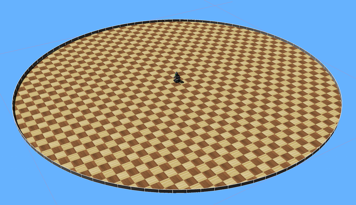
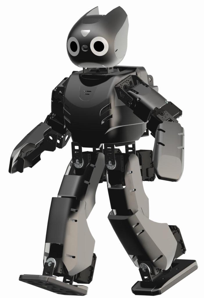
4.1 The continuous MDP

We start by defining a continuous $M_{\infty}$ for the robot problem. A state $s\in S_{\infty}$ is of the form $s=(w_{1},\cdots,w_{23})\in\mbox{$I\!\!R$}^{23}$, where $(w_{1},w_{2},w_{3})$ give the position of the robot’s center of mass and $(w_{4},\cdots,w_{23})$ are the current positions of the robot’s 20 joint motors. We define the domain of each dimension as follows: since the radius of the arena is 5 meters, $w_{1},w_{2}\in[-5,5]$; since the robot’s height is 0.454 meters, $w_{3}\in[0,0.4]$ (we do not expect the robot’s center of mass to be higher than 0.4). Each joint motor has its specific range of mobility, which determines the domain of the corresponding dimension. For example, $w_{5}\in[-3.14,2.85]$ represents the current position of the robot’s left shoulder. The mobility range for all joint motors are intervals in $[-\pi,\pi]$.

The basic actions $a\in A_{B}$ are of the form $a=(v_{1},\cdots,v_{20})\in\mbox{$I\!\!R$}^{20}$, where $v_{i}$ is the target position for the robot’s $i$th joint motor. The domain of each dimension is the mobility range for the corresponding joint motor. For example, $v_{2}$, which corresponds to the left shoulder, has mobility range $[-3.14,2.85]$; $v_{2}=2.85$ means to move the robot’s left shoulder forward as far as possible. Since walking is composed of repeated short movements that are typically no longer than half a second, we set $T=0.512$ seconds. Thus, $A_{\infty}$, the set of useful actions, consists of piecewise continuous functions that map from time to basic actions and comply with the robot’s hardware and software limitations, of length $t<0.512$ seconds.

We now define $R_{\infty}$ and $P_{\infty}$. Intuitively, the robot obtains a reward for gaining distance from the center of the arena. If the coordinates of the center of the arena are given by $s_{0}=(s_{0}[1],s_{0}[2])$, then $R_{\infty}(s_{1},s_{c},a)=dis(s_{0},s_{c}(|a|))-dis(s_{0},s_{1})$, where $dis(s_{0},s_{1})=\sqrt{(s_{0}[1]-s_{1}[1])^{2}+(s_{0}[2]-s_{1}[2])^{2}}$ is the $L_{2}$-norm distance between $s_{0}$ and $s_{1}$ on the $(x,y)$-plane. The reward could be negative, for example, if the robot moves back towards the center of the arena.

By definition, $P_{\infty}(s_{1},\cdot,a)$ is a probability distribution over state sequences of length $|a|$ starting at $s_{1}$. For example, if the robot slowly moves its right leg forward while staying balanced, the state path taken by the robot is a deterministic path. On the other hand, if $a$ is the action of turning around quickly, $P_{\infty}(s,\cdot,a)$ is distribution over various ways of falling down.

4.2 Discretizations

We now define $M_{i}$ and $M_{i}^{\prime}$. In our experiments we considered only levels 2 and 3 (level 1 is uninteresting since it has just one state and one action), so these are the only levels that we describe in detail here. (These turn out to suffice to get interesting walking behaviors.) At these levels, we discretized more finely the joints corresponding to the left and right upper and lower leg joints and the left and right ankle joints, since these turn out to be more critical for walking. (These are components $(w_{14},\cdots,w_{19})$ in the state tuples and $(v_{11},\cdots,v_{16})$ in basic-actions tuples.) We call these the relevant dimensions. We assume that the six relevant state and actions components have $i$ possible values at level $i$, for $i=2,3$, as does $w_{3}$, since this describes how high off the ground the robot is (and thus, whether or not it has fallen). All other dimensions take just one value. We took $t_{2}=t_{3}$ to be $128$ms. Since $T=0.512$s, an action contains at most $\left\lfloor T/t_{i}\right\rfloor=4$ basic actions.

$A_{\infty 0}$ is the set of preprogrammed actions. We preprogram the robot with a simple sitting action that lets the robot slowly return to its initial sitting gesture. When we consider apprenticeship learning, we also assume that the robot is preprogrammed with a “stand-up” action, that enables it to stand up from its initial sitting position. (Intuitively, we are assuming that the expert taught the robot how to stand up, since this is useful after it has fallen.)

$A_{i}^{\prime}$ is the set of potential actions at level $i$. Given our assumptions, for $i=2,3$, at level $i$, there are $(i^{6})^{4}$ potential actions (there are $i$ possible values for each of the six relevant dimensions, and each action is a sequence of four basic actions). Thus, at level 3, there are $(3^{6})^{4}=$282,429,536,481 potential actions. As we mentioned, a useful action is an action that moves the robot without making it lose control. Here, an action is useful if it moves the robot without resulting in the robot falling down. At both levels 2 and 3, more than 80 useful actions were found in our experiments. The most efficient action found at level 3 was one where the right leg moves backwards, immediately followed by the left leg, in such a way that the robot maintains its balance at all times. By way of contrast, turning the body quickly makes the robot lose control and fall down, so is useless.

For $s_{1}\in S_{i}$, $a\in A_{i}$, and $s_{c}\in Q_{i}^{|a|}$, $P_{i}(s_{1},s_{c},a)$ is the normalized probability of traversing a state sequence that is $d_{i}$ close to $s_{c}$, a sequence of states in $S_{i}$, where we define $d_{i}=\frac{12\pi}{i}+28\pi+20.4$. So $d_{i}$ decreases in $i$, and discretizations at a higher level better approximate the continuous problem. All basic actions in $A_{B}$ are within distance $d_{i}$ of a basic action in $A_{Bi}$ and all states in $S$ are within $d_{i}$ of a state in $S_{i}$. Let $s\in S$, and let $s_{i}$ be the closest state to $s$ in $S_{i}$. It is easy to check that $d(s,s_{i})\leq d_{i}$ for $i=2,3$.

The $D_{i}$ function depends on the exploration method used to discover new actions. In our experiment, we used two exploration methods: brute-force exploration and apprenticeship-learning exploration.

At discretization level $i$, using brute-force exploration, we have $D_{i}(|A_{i}|,t)=\frac{|A_{i}|}{|A_{i}^{\prime}|}$, since there are $|A_{i}|$ useful actions and $|A_{i}^{\prime}|$ potential actions, and we test an action at random. With apprenticeship learning, we used following hints from a human expert to increase the probability of discovering new actions: (a) a sequence of moving directions that, according to the human expert, resembles human walking; (b) a preprogrammed stand-up action; (c) the information that an action that is symmetric to a useful action is also likely to be useful (two actions are symmetric if they are exactly the same except that the target values for the left joints and those for the right joints are switched). We also use a different discretization: the ankle joint was discretized into 10 values. The human expert suggests more values in the ankle joints because whether or not the robot falls depends critically on the exact ankle joint position. These hints were provided before the policy starts running; the discretization levels are set then too. There were no further human-robot interactions.

4.3 Experiments

For our experiments, we simulated DARwIn OP, a commercially available humanoid robot. The simulations were conducted on Webots PRO platform 8.2.1 using a MacBook Pro with 2.8GHz Intel Core i7 Processor, 16GB 1600 MHz DDR3 memory, 0.5TB Flash Storage Mac HD, on OS X Yosemite 10.10.5. We modeled the robot walking problem as an MDPU, and implemented the URMAX algorithm to solve the problem using programming language Python 2.7.7.

As we said, given the number of actions involved, we conducted experiments only for discretization level 2 and 3. Both sufficed to enable the robot to learn to walk, using a generous notion of “walk”—more precisely, they sufficed to enable the robot to learn to locomote to the boundary of the arena. As mentioned, two exploration methods were used: brute-force exploration and apprenticeship-learning exploration. One trial was run for brute-force exploration at each of levels 2 and 3, and one trial was run for apprenticeship learning at level 2. Each trial took 24 hours. More than 15 stable gaits were found in total, where a gait is stable if it enables the robot to move from the center of the arena to the boundary without falling. In addition, more than 400 useful actions were found. The best gait among all stable gaits achieved a velocity of 0.084m/s, which seems reasonable, given that the best known walking speed of DARwIn-OP is 0.341m/s [Budden et al. 2013]. Given more time to experiment, we would expect the performance to improve further.

	Brute-force (level 2)	Brute-force (level 3)	Apprenticeship learning (level 2)
$|S_{i}|$	130	1460	3200
$|A_{Bi}|$	64	729	1600
$|A_{i}|$	16777216	282429536481	6553600000000
$t_{i}$ (ms)	124	124	124
Length of action (ms)	496	496	496
Execution time (hours)	24	24	24
Best avg rwd (m/action)	0.043486	0.067599	0.083711
Num of useful actions found	131	89	180

Table 1: Performance comparisons.

Figure 2: A backward gait (from left to right).

Figure 3: A forward gait (from left to right).

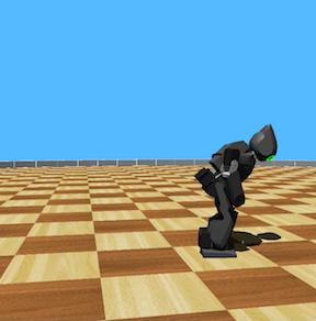
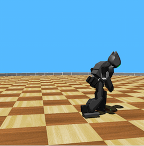
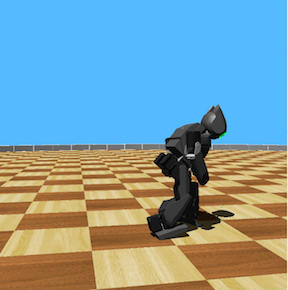
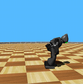
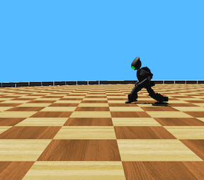
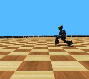
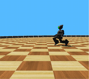
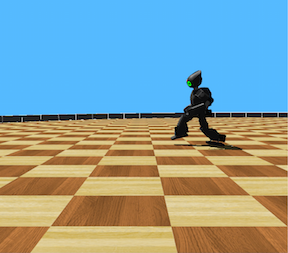
The robot successfully learned gaits of various styles, including both forward and backward gaits (see Figures 2 and 3), both efficient and inefficient gaits, gaits that resemble human walking and the ones that do not. Somewhat surprisingly, the best gait actually walks backwards. (Videos of some of the gaits and a demo of the learning process can be found at https://youtu.be/qW51iInpdV0.) As shown in Table 1, as the discretization level increases, both the velocity of the best gait and the number of useful actions found increase. This agrees with the expectation that finer discretization better approximates the continuous problem, and thus gets an expected reward closer to the optimal reward of the continuous problem. Apprenticeship learning resulted in more useful actions than the brute-force exploration and in gaits with a higher average reward. Again, this is hardly surprising; the hints provided by the human expert increases the probability of finding useful actions. On the other hand, when the expert gives “bad” hints, the robot performs worse than with brute-force exploration.

With regard to comparisons under the same setting, we implemented two baseline comparisons for bipedal walking. The first tries random sequences of actions; the second searches for useful actions and then repeats each useful action in an attempt to find stable gaits. (The motivation for repeating actions is that human-like walking is in fact a rhythmic/cyclic movement of a repeated action.) Using the same setting as our experiments with URMAX, the first baseline found no stable gait in 24 hours, and the maximum distance the robot traveled before falling down was 0.342 meters; the second baseline found one stable gait in 24 hours, and the maximum distance traveled was 5 meters (the maximum distance possible from the center of the arena to the boundary) with a speed of 0.0058 m/s. Our approach found several stable gaits at each discretization level and the distance traveled using each stable gait is 5 meters with a maximum speed of 0.083m/s (10 times better than the second baseline).

Our approach, using MDPUs, requires no knowledge on the kinematics of the robot other than the number of joints and the moving range of each joint. Moreover, it makes no assumptions about the moving pattern of the resulting gait; for example, we do not assume that a gait must be cyclic, or symmetric between left and right joints, nor do we specify the length of a gait. Although we do specify the length of a useful action, a gait could be composed of a single or multiple useful actions. Given the few assumptions and little prior knowledge assumed, the performance of the robot seems quite reasonable. More importantly, the experiment proves that the use of MDPUs enables the robot to learn useful new maneuvers (walking, in this case) by itself, with minimum human input.

5 RELATED WORK

There has been work on optimal policy learning in MDPs using computational resources. Kearns and Singh’s [?] $E^{3}$ algorithm guarantees polynomial bounds on the resources required to achieve near-optimal return in general MDPs; variants and extensions of this work can be found in [Brafman and Tennenholtz 2002, Kakade et al. 2003, Kearns and Koller 1999]. However, algorithms such as $E^{3}$ usually require the exploration of the entire MDP state/action space. This becomes impractical in our setting, where the number of actions is extremely large. In such cases, several exploration methods have been employed to help find useful actions. For example, Abbeel and Ng [?] utilize a teacher demonstration of the desired task to guide the exploration; Dearden et al. [?] utilize the value of information to determine the sequence of exploration. Guestrin et al. [?] make use of approximate linear programming, and focus on exploring states that directly affect the results of the planner; Kakade et al. [?] proved that in certain situations, the amount of time required to compute a near-optimal policy depends on the covering number of the state space, where, informally, the covering number is the number of neighborhoods required for accurate local modeling; Other papers (e.g., [Dean et al. 1998, Hauskrecht et al. 1998]) consider MDPs with large action spaces.

We are far from the first to consider MDPs with continuous time. For example, semi-MDPs (SMPDs) and continuous-time MDPs have continuous time [Puterman 1994]. However, these models have discrete actions that can be taken instantaneously, and do not consider continuous actions taken over some duration of time. In Markov decision drift processes [Hordijk and Van der Duyn Schouten 1984], the state does not have to stay constant between successive actions (unlike an SMDP), and can evolve in a deterministic way according to what is called a drift function. But Markov decision drift processes do not have actions with probabilistic outcomes that take place over an interval of time. Hordijk and van der Duyn Schouten [?] make significant use of discrete approximations to compute optimal policies, just as we do. There has also been work on MDPs with continuous state space and action space (e.g., [Antos and Munos 2007, Feng et al. 2004]), but with discrete time. For our applications, we need time, space, and actions to be continuous; this adds new complications. In control theory, there are methods for controlling continuous time systems where system transitions are linear function of state and time [Zinober 1989]. These can be extended to non-linear systems [Khalil 2002]. However, the transitions in these systems are usually deterministic, and they do not deal with rewards or policies. Sutton, Precup, and Singh [?] consider high-level actions (which they call options) that are taken over a duration of time (such as “opening a door”), but they view time as discrete, which significantly simplifies the model. Rachelson, Garcia, and Fabiani [?] consider continuous actions over some time interval, however, they assume there are decision epochs, which are the only time points where rewards are considered. In our model, the rewards depend on the entire state sequence that the system traverses through while an action is taken. While this makes the model more complicated, it seems more appropriate for the problems of interest to us.

There has also been a great deal of work on bipedal robot walking, since it is a fundamental motor task for which biological systems significantly outperform current robotic systems [Tedrake et al. 2005]. There have been three main approaches for solving the task:

• The first approach describes the kinematics of the robot in detail using non-linear and linear equation systems, then solves these systems to obtain desirable trajectories. See, for example, [Huang et al. 2001, Gon alves and Zampieri 2006, Kajita et al. 2003, Kim et al. 2007, Strom et al. 2010, Xue et al. 2012].

• The second approach uses genetic algorithms [Cheng and Lin 1997, Hasegawa et al. 2000, Picado et al. 2009]. The traits describing a gait are taken to be the genes in a genetic algorithm. Different gaits (i.e., settings of the parameters) are evaluated in terms of features such as stability and velocity; The most successful gaits are retained, and used to produce the next generation of gaits through selection, mutation, inversion, and crossover of their genes. This approach can also be used for to learn quadrupedal and nine-legged walking. See, for example, [Chernova and Veloso 2004, Parker and Tarimo 2011, Parker et al. 2011, Zykov et al. 2004].

• The third approach uses gradient learning, which starts with either a working gait or a randomly initialized gait. It then improves the gait’s performance by changing its parameters, using machine-learning methods (such as neural networks) to find the most profitable set of changes in the parameters. See, for example, [Budden et al. 2013, Kim and Uther 2003, Schulman et al. 2015, Tedrake et al. 2005]. this approach is also used in quadrupedal walking [Kohl and Stone 2004].

Since the first approach requires a full description of the robot’s kinematics, as well as composing and solving a non-linear system, it requires a great deal of human input. Moreover, its application is limited to walking problems. The approach is unable to produce gaits other than those specified by human (e.g., to walk forward by stepping forward the left and the right legs in turn under a specific speed). Both the second and the third approach require little human input (when starting from random gaits), and may produce a variety of gaits. Both also have the potential to be generalized to problems other than bipedal walking. However, both are heuristic search algorithms, and have no theoretical guarantee on their performance. In contrast, our method produces a variety of gaits, provides a general framework for solving robotic problems, and produces a near-optimal policy in the limit. Moreover, our method requires minimum human input, although, as the experiments show, it does better with more human input.

A comparison of our method and the genetic algorithm may provide insights into both methods. Although the two approaches seem different, the searching process made possible by selection, mutation, inversion, and crossover in a genetic algorithm can be viewed as a special case of the explore action in an MDPU. Conversely, the explore action in an MDPU for the robot can be roughly viewed as searching for a set of genes of unknown length (since a gait can be understood as a continuous action over an uncertain amount of time, composed of one or more shorter actions, where each shorter action is described by a set of parameters). Our approach can be viewed as being more flexible than a genetic algorithm; in a genetic algorithm, the length of the chromosome (i.e., the number of parameters that describe the gait) is fixed; only their values that give the best performance are unknown.

The recent work of Mordatch et al [?] also provides a general approach for reinforcement learning in robot tasks. Like us, they require prior knowledge only of the mobility range of each of the robot’s joints, and not their kinematics; they also model the problem as an MDP. Their goal is to find an optimal trajectory (i.e., a sequence of states), such that when followed, performs a desired task (such as reaching out the robot’s hand to a desired position) with minimal cost. They use neural networks to solve the cost-minimization problem. Thus, their approach does not have any guarantees of (approximate) optimality of the performance. Moreover, the complexity of their approach grows quickly as the length of the trajectory grows (while ours is polynomial in the number of useful actions, states visited, and the difficulty of discovering new actions, and thus is not significantly affected by the length of the trajectory). That said, Mordatch et al.’s method has successfully learned a few relatively simple tasks on a physical DARwIn OP2 robot, including hand reaching and leaning the robot’s torso to a desired position [Mordatch et al. 2016], although it has not yet been applied to walking.

6 CONCLUSION

We have provided a general approach that allows robots to learn new tasks on their own. We make no assumptions on the structure of the tasks to be learned. We proved that in the limit, the method gives a near-optimal policy. The approach can be easily applied to various robotic tasks. We illustrated this by applying it to the problem of bipedal walking. Using the approach, a humanoid robot, DARwIn OP, was able to learn various walking gaits via simulations (see https://youtu.be/qW51iInpdV0 for a video). We plan to apply our approach to more robotic tasks, such as learning to run and to walk up and down stairs. We believe the process will be quite instructive in terms of adding useful learning heuristics to our approach, both specific to these tasks and to more general robotic tasks. We are also interested in having the robot simulate learning to walk in the same way a baby does, for example, by limiting the robot’s abilities initially, so that it must crawl before it walks. Part of our interest lies in seeing if such initial limitations actually make learning more efficient.

Acknowledgments: The work of Halpern and Rong was supported in part by NSF grants IIS-0911036 and CCF-1214844, and by AFOSR grant FA9550-12-1-0040, and ARO grant W911NF-14-1-0017. The work of Saxena was supported in part by a Microsoft Faculty Fellowship.

Appendix

In this appendix, we provide proofs of Theorems 3.1 and 3.1. We start with Theorem 3.2. We repeat the statement of the theorem for the reader’s convenience.

Theorem 3.2: Using an exploration method where $D_{i}(1,t)\geq\beta$ for all $i,t>0$ where $\beta\in(0,1)$ is a constant, for any $\alpha>0$ and $0<\delta<1$, the robot can obtain an $\alpha$-optimal policy to $M_{\infty}$ with probability at least $1-\delta$ in time polynomial in $l$, $|A_{l}|$, $|S_{l}|$, $1/\beta$, $1/\alpha$, $1/\delta$, $R_{\max}$ and $T^{l}$, where $l$ is the smallest $i$ such that the optimal policy for $M_{i}^{\prime}$ is $(\alpha/2)$-optimal to $M_{\infty}$, $R_{\max}^{l}$ is the maximum reward (that a transition can obtain) in $M_{l}^{\prime}$, and $T^{l}$ is the $\epsilon$-return mixing time for $M_{l}^{\prime}$.

Figure 4: The diagonal execution of URMAX.

Proof: Since $D_{i}(1,t)\geq\beta$ for $i\geq 1$, for all levels $i\geq 1$, we have $\Psi(t)\geq\beta\cdot t\geq\beta\ln(t)$ for all $t\geq 1$. By Theorem 2.5, for each level $i$, with probability at least $1-\delta$, we can obtain a policy $\pi_{i}$ that is $(\alpha/2)$-optimal for $M_{i}^{\prime}$ in time polynomial in $|A_{i}|$, $|S_{i}|$, $1/\beta$, $2/\alpha$, $1/\delta$, $R_{\max}^{i}$, and $T^{i}$ using the URMAX algorithm, where $R_{\max}^{i}$ is the maximum reward in $M_{i}^{\prime}$ and $T^{i}$ is the $(\alpha/2)$-return mixing time for $M_{i}^{\prime}$.

However, we are not interested in obtaining a near-optimal policy for $M_{i}^{\prime}$; we want a near-optimal policy for $M_{\infty}$. Let $l$ be the smallest $i$ such that the optimal policy for $M_{i}^{\prime}$ is $(\alpha/2)$-optimal for $M_{\infty}$. Such a level $l$ must exist, due to the continuity of the reward and transition functions of $M_{\infty}$. For suppose that $\pi$ is the optimal policy in $M_{\infty}$. By continuity, there exists a level $l$ and a policy $\pi^{\prime}$ at level $l$ such that the expected reward of $\pi^{\prime}$ is within $\alpha/2$ of that of $\pi$. But then the optimal policy at level $l$ must have expected reward within $\alpha/2$ of that of $\pi$. Since $\pi_{l}$ is $(\alpha/2)$-optimal for $M_{l}^{\prime}$, and the optimal policy for $M_{l}^{\prime}$ is $(\alpha/2)$-optimal for $M_{\infty}$, $\pi_{l}$ must be $\alpha$-optimal for $M_{\infty}$.

Thus, if we knew $l$ and the values of all the relevant parameters, then by running URMAX at each level from 1 to $l$, we could obtain an $\alpha$-optimal policy for $M_{\infty}$ in time polynomial in $l$, $|S_{l}|$, $1/k$, $2/\epsilon$, $1/\delta$, $R_{\max}^{j}$, $|A_{j}|$ and $T^{j}$ for all $j\in[1,l]$. Note that we include $|A_{j}|$ and $T^{j}$ for all $j\in[1,l]$ here. This is because we did not assume each discretization level $j+1$ is a refinement of the discretization level $j$; thus, it could happen that $R_{\max}^{l}<R_{\max}^{j}$ for some $j<l$, or $|A_{l}|<|A_{j}|$ for some $j<l$, or that $T^{l}<T^{j}$ for some $j<l$. However, we show below that we actually need only $R_{\max}^{l}$, $|A_{l}|$, and $T^{l}$ (instead of all $R_{\max}^{j}$, $|A_{j}|$, and $T^{j}$).

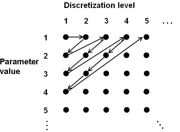
The problem with the approach described in the previous paragraph is that we do not know $l$ nor the values $|S_{l}$, $|A_{j}|$, $T^{j}$ and $R_{\max}^{j}$ for $j\in[1,l]$. We solve this problem just as HRS solved the analogous problem when running the URMAX algorithm (see [Halpern et al. 2010]): we diagonalize. Specifically, we start running URMAX at discretization level 1 under the assumption that the parameters ($|A_{1}|$, $|S_{1}|$, $R_{\max}^{1}$, $|S_{1}|$) all have value 1. level 2 with the parameters set to 1, and run URMAX at level 1 with parameters set to 2; and so on. The process is described in Figure 4. A similar approach is used by HRS to increase the value of unknown parameters. We call running URMAX at a specific particular discretization level using a particular setting of the parameters an iteration of URMAX. For example, running URMAX at discretization level 3 with the parameters set to 4 is one iteration of URMAX.

To deal with the fact that we do not know $l$, we always keep track of the current candidate for best policy. (That is, the policy that is optimal given the current set of assumptions about values of the parameters, given the actions that have been discovered and our current estimate of the transition probabilities.) At the end of each iteration of URMAX we run the current candidate optimal policy a sufficient number of times so as to guarantee that the average payoff of URMAX is close to optimal, if the current candidate optimal policy is indeed $\alpha$-optimal. Eventually, URMAX will reach a stage where it is exploring discretization level $l$ using values for the parameters $|A_{l}|$, $|S_{l}|$, $R_{\max}^{l}$ and $T^{l}$ that are at least as high as the actual values. At that point, the candidate for optimal policy is almost certain to be $\alpha$-optimal for $M_{\infty}$. (Recall that $l$ is defined to be the discretization level at which the optimal policy is $\alpha/2$-optimal for $M_{\infty}$.) After this point, we always run a policy that is at least $\alpha$-optimal to $M_{\infty}$. Note that this happens even if we do not know the value of $l$ or any of the relevant parameters.

Thus, although URMAX runs forever, from some point in time it has discovered an $\alpha$-optimal algorithm. Moreover, due to the “diagonal” manner in which URMAX is run, the candidate optimal policy is (with probability $1-\delta$) $\alpha$-optimal after time polynomial in $l$, $|A_{l}|$, $|S_{l}|$, $T^{l}$, $R_{\max}^{l}$, $k$, $1/\delta$, and $2/\alpha$. From that point on, we are guaranteed to run policies that are $\alpha$-optimal for $M_{\infty}$.  

Theorem 3.1: Using brute-force exploration, for any $\alpha>0$ and $0<\delta<1$, a DM can find an $\alpha$-optimal policy in $M_{\infty}$ with probability at least $1-\delta$ in time polynomial in $l$, $|A_{l}^{\prime}|$, $|S_{l}|$, $1/\alpha$, $1/\delta$, $R_{\max}^{l}$ and $T^{l}$, where $l$ is the least $i$ such that the optimal policy for $M_{i}^{\prime}$ is $(\alpha/2)$-optimal for $M_{\infty}$, $R_{\max}^{l}$ is the maximum reward (that a transition can obtain) in $M_{l}^{\prime}$, and $T^{l}$ is the $\epsilon$-return mixing time for $M_{l}^{\prime}$.

Proof: At any discretization level, there are only finitely many possible actions. Since the brute force exploration examines all possible actions at each level, it is guaranteed to find all useful actions, and thus the near-optimal policy for that level.

We apply the URMAX algorithm diagonally as described in the Proof for Theorem 3.2, so that sooner or later, we will reach the discretization level $i$ such that the optimal policy for $M_{i}^{\prime}$ is $\epsilon$-close to $P^{*}$, and run URMAX in that level with parameters values no less than the real values of $|A_{i}|$, $|S_{i}|$, $T_{i}$ and $R_{\max}^{i}$. Thus, we are guaranteed to obtain an $\epsilon$-near-optimal policy.

References

- Abbeel and Ng 2005 Abbeel, P. and A. Y. Ng (2005). Exploration and apprenticeship learning in reinforcement learning. In Proc. 22nd Int. Conf. on Machine Learning (ICML ’05), pp. 1–8.
- Antos and Munos 2007 Antos, A. and R. Munos (2007). Fitted Q-iteration in continuous action-space MDPs. In Advances in Neural Information Processing Systems 20 (Proc. of NIPS 2007), pp. 9–16.
- Brafman and Tennenholtz 2002 Brafman, R. I. and M. Tennenholtz (2002). R-MAX: A general polynomial time algorithm for near-optimal reinforcement learning. Journal of Machine Learning Research 3, 213–231.
- Budden et al. 2013 Budden, D., J. Walker, M. Flannery, and A. Mendes (2013). Probabilistic gradient ascent with applications to bipedal robot locomotion. In Australasian Conference on Robotics and Automation (ACRA 2013), pp. 37–45.
- Cheng and Lin 1997 Cheng, M.-Y. and C.-S. Lin (1997). Genetic algorithm for control design of biped locomotion. Journal of Robotic Systems 14(5), 365–373.
- Chernova and Veloso 2004 Chernova, S. and M. Veloso (2004). An evolutionary approach to gait learning for four-legged robots. In Proc. International Conference on Intelligent Robots and Systems (IROS 2004) Vol. 3, pp. 2562 – 2567.
- Dean et al. 1998 Dean, T., K. Kim, and R. Givan (1998). Solving stochastic planning problems with large state and action spaces. In Proc. 4th Int. Conf. on Artificial Intelligence Planning Systems, pp. 102–110.
- Dearden et al. 1999 Dearden, R., N. Friedman, and D. Andre (1999). Model based bayesian exploration. In Proc. 15th Conf. on Uncertainty in AI (UAI ’99), pp. 150–159.
- Feng et al. 2004 Feng, Z., R. Dearden, N. Meuleau, and R. Washington (2004). Dynamic programming for structured continuous Markov decision problems. In In Proc. 20th Conf. on Uncertainty in Artificial Intelligence, pp. 154–161.
- Gon alves and Zampieri 2006 Gon alves, J. B. and D. E. Zampieri (2006, 12). An integrated control for a biped walking robot. Journal of the Brazilian Society of Mechanical Sciences and Engineering 28, 453 – 460.
- Guestrin et al. 2002 Guestrin, C., R. Patrascu, and D. Schuurmans (2002). Algorithm-directed exploration for model-based reinforcement learning in factored mdps. In Proc. International Conference on Machine Learning (ICML 2002), pp. 235–242.
- Halpern et al. 2010 Halpern, J. Y., N. Rong, and A. Saxena (2010). MDPs with unawareness. In Proc. 26th Conf. on Uncertainty in AI (UAI ’10), pp. 228–235.
- Hasegawa et al. 2000 Hasegawa, Y., T. Arakawa, and T. Fukuda (2000). Trajectory generation for biped locomotion robot. Mechatronics 10, 67–89.
- Hauskrecht et al. 1998 Hauskrecht, M., N. Meuleau, L. Kaelbling, T. Dean, and C. Boutilier (1998). Hierarchical solution of Markov decision processes using macro-actions. In Proc. 14th Conf. on Uncertainty in AI (UAI ’98), pp. 220–229.
- Hordijk and Van der Duyn Schouten 1984 Hordijk, A. and F. A. Van der Duyn Schouten (1984). Discretization and weak convergence in Markov decision drift processes. Mathematics of Operations Research 9, 112–141.
- Huang et al. 2001 Huang, Q., K. Yokoi, S. Kajita, K. Kaneko, H. Arai, N. Koyachi, and K. Tanie (2001). Planning walking patterns for a biped robot. IEEE Transactions on Robotics and Automation 17, 280–289.
- Kajita et al. 2003 Kajita, S., F. Kanehiro, K. Kaneko, K. Fujiwara, K. Harada, K. Yokoi, and H. Hirukawa (2003). Biped walking pattern generation by using preview control of zero-moment point. In Proc. International Conference on Robotics and Automation (ICRA 2003), Vol. 2, pp. 1620 – 1626.
- Kakade et al. 2003 Kakade, S., M. Kearns, and J. Langford (2003). Exploration in metric state spaces. In Proc. 20th Int. Conf. on Machine Learning (ICML ’03), pp. 306–312.
- Kearns and Koller 1999 Kearns, M. and D. Koller (1999). Efficient reinforcement learning in factored MDPs. In Proc. Sixteenth Int. Joint Conf. on Artificial Intelligence (IJCAI ’99), pp. 740–747.
- Kearns and Singh 2002 Kearns, M. and S. Singh (2002). Near-optimal reinforcement learning in polynomial time. Machine Learning 49(2-3), 209–232.
- Khalil 2002 Khalil, H. K. (2002). Nonlinear Systems. Prentice-Hall.
- Kim et al. 2007 Kim, J., I. Park, and J. Oh (2007). Walking control algorithm of biped humanoid robot on uneven and inclined floor. Journal of Intelligent and Robotic Systems 48(4), 457–484.
- Kim and Uther 2003 Kim, M. S. and W. Uther (2003). Automatic gait optimisation for quadruped robots. In Proc. Australasian Conference on Robotics and Automation (ACRA).
- Kohl and Stone 2004 Kohl, N. and P. Stone (2004). Policy gradient reinforcement learning for fast quadrupedal locomotion. In Proc. IEEE International Conference on Robotics and Automation (ICRA 2004), pp. 2619–2624.
- Mordatch et al. 2016 Mordatch, I., N. Mishra, C. Eppner, and P. Abbeel (2016). Combining model-based policy search with online model learning for control of physical humanoids. Preprint, http://www.eecs.berkeley.edu/ igor.mordatch/darwin/paper.pdf.
- Parker and Tarimo 2011 Parker, G. and W. Tarimo (2011). Using cyclic genetic algorithms to learn gaits for an actual quadruped robot. In Proc. IEEE International Conference on Systems, Man, and Cybernetics (SMC 2011), pp. 1938 – 1943.
- Parker et al. 2011 Parker, G. B., W. T. Tarimo, and M. Cantor (2011). Quadruped gait learning using cyclic genetic algorithms. In Proc. IEEE Congress on Evolutionary Computation (CEC 2011), pp. 1529 – 1534.
- Picado et al. 2009 Picado, H., M. Gestal, N. Lau, L. P. Reis, and A. M. Tome (2009). Automatic generation of biped walk behavior using genetic algorithms. In Proc. 10th International Work-Conference on Artificial Neural Networks, pp. 805–812.
- Puterman 1994 Puterman, M. L. (1994). Markov Decision Processes. John Wiley and Sons, Inc.
- Rachelson et al. 2008 Rachelson, E., F. Garcia, and P. Fabiani (2008). Extending the bellman equation for MDPs to continuous actions and continuous time in the discounted case. In 10th Int. Symp. on Artificial Intelligence and Mathematics.
- Schulman et al. 2015 Schulman, J., S. Levine, P. Moritz, M. Jordan, and P. Abbeel (2015). Trust region policy optimization. In Proc. 31st International Conference on Machine Learning (ICML ’15), pp. 1889–1897.
- Strom et al. 2010 Strom, J., G. Slavov, and E. Chown (2010). Omnidirectional walking using ZMP and preview control for the nao humanoid robot. In RoboCup 2009: Robot Soccer World Cup XIII, pp. 378–389.
- Sutton et al. 1999 Sutton, R., D. Precup, and S. Singh (1999). Between MDPs and semi-MDPs: A framework for temporal abstraction in reinforcement learning. Artificial Intelligence 112, 181–211.
- Tedrake et al. 2005 Tedrake, R., T. W. Zhang, and H. S. Seung (2005). Learning to walk in 20 minutes. In Proc. Fourteenth Yale Workshop on Adaptive and Learning Systems.
- Xue et al. 2012 Xue, F., X. Chen, J. Liu, and D. Nardi (2012). Real time biped walking gait pattern generator for a real robot. In T. Röfer, N. M. Mayer, J. Savage, and U. Saranlı (Eds.), RoboCup 2011: Robot Soccer World Cup XV, pp. 210–221. Springer.
- Zinober 1989 Zinober, A. S. (1989). Deterministic control of uncertain systems. In Proc. Int. Conf. on Control and Applications (ICCON ’89), pp. 645–650.
- Zykov et al. 2004 Zykov, V., J. Bongard, and H. Lipson (2004). Evolving dynamic gaits on a physical robot. In Proc. Genetic and Evolutionary Computation Conference, Late Breaking Paper (GECCO’04).