Sensor Networks TDOA Self-Calibration: 2D Complexity Analysis and Solutions
Abstract
Given a network of receivers and transmitters, the process of determining their positions from measured pseudoranges is known as network self-calibration. In this paper we consider 2D networks with synchronized receivers but unsynchronized transmitters and the corresponding calibration techniques, known as Time-Difference-Of-Arrival (TDOA) techniques. Despite previous work, TDOA self-calibration is computationally challenging. Iterative algorithms are very sensitive to the initialization, causing convergence issues. In this paper, we present a novel approach, which gives an algebraic solution to two previously unsolved scenarios. We also demonstrate that our solvers produce an excellent initial value for non-linear optimisation algorithms, leading to a full pipeline robust to noise.
Index Terms— Time Difference of Arrival, Sensor Networks Calibration, Minimal Problems
1 Introduction
Wireless Sensor Networks have been widely studied [18] and have been successfully applied to several domains, such as positioning [15], mapping [17], microphone array calibration [12] and beamforming [11]. In order to be properly used, the network must first be calibrated, i.e. the positions of its nodes need to be determined. This can be done e.g. using transmitters at a known position and trilaterating the network nodes. However, several applications require simultaneous localization of both receivers and transmitters [10]. This is known as network self-calibration [9, 18] and it is the main theme of this paper.
Let us consider a network with receivers and transmitters, shortly denoted as . From the measurements equations will be available to solve the self-calibration problem. Now, we consider two different scenarios:
-
•
Synchronized RXs and TXs: In this situation, the time instants at which the signal is transmitted and measured are known and hence the distances between RX and TX are measured. For each pair of receiver-transmitter, the following polynomial equation is obtained
(1) where is the measured range and is the distance between the receiver located at and the transmitter located at . In total we will have degrees of freedom (DoF), where denotes the spatial dimension () and is the Gauge freedom ( in 2D and in 3D). Since we measure only distances, the positions can be recovered only up to a Euclidean transformation. Practically, this means that the coordinate systems in which we solve the coordinates can be chosen freely, reducing the degrees of freedom. This formulation is known as Time-Of-Arrival (TOA).
-
•
Synchronized RXs and unsynchronized TXs: In this situation, all receivers will measure the time of arrival in the same clock frame. For each pair of transmitter-receiver, the following polynomial equation is obtained
(2) As equation (2) shows, each transmitter introduces an extra unknown , the time offset between the transmitter local clock and the receivers clock. The total number of degrees of freedom will thus be . This formulation is known as Time-Difference-Of-Arrival (TDOA).
The above mentioned equations could be solved by numerical iterative methods [14, 2]. These approaches, however, can suffer from several issues such as getting stuck in local minima, slow convergence and sensitivity to outliers. It has been shown that algebraic non-iterative approaches can achieve higher accuracies [5, 6, 1, 4, 8]. Furthermore, using the algebraic solution as initial value for iterative methods allows a faster and more accurate convergence.
This paper focuses on TDOA, particularly to the 2D case (). The total number of DoF will thus be . The configurations for which the number of DoF equals the number of equations are referred to as minimal configurations and the problems of network self-calibration with the minimum amount of receivers and transmitters are called minimal problems. The minimal configurations for 2D TDOA are 6r/3s and 4r/5s. Previous work developed algebraic solvers for non-minimal cases, such as 7r/6s, 5r/6s [6] and 8r/4s [13], however the minimal problems cannot be solved algebraically yet.
| 3 | 4 | 5 | 6 | |
|---|---|---|---|---|
| 4 | u | u | M | - |
| 5 | u | - | - | X |
| 6 | M | O | * | * |
| 7 | - | X | * | * |
| 8 | - | * | * | * |
| 9 | O | * | * | * |
In this paper, we fill the gap towards minimal problems, proposing a new approach, able to solve two previously unsolved configurations: and , as summarized in Table 1. Opposed to previous methods, where TDOA was tackled by first solving for the offsets and then solving the remaining TOA problem, our approach combines TOA and TDOA ideas and jointly solves both offsets and positions, reducing the overall computation load of the pipeline. Furthermore, we provide a quantitative estimate of the computational complexity of several unsolved configurations.
The paper is structured as follows: in Section II the current state of the art of TOA and TDOA solving techniques is reviewed. In Section III our proposed method is explained, and our solvers are benchmarked in Section IV. Finally, conclusions are drawn in Section V.
2 Related Work
In these sections, we review the state-of-the-art techniques that have been used to algebraically solve TOA and TDOA so far.
2.1 TOA
From the distances we can define the compaction matrix [5] such that
| (3) |
With algebraic manipulation, it can be shown that the following factorization holds
| (4) |
where for and similarly for .
This factorization is not unique, suppose we have a factorization . Clearly, for each full-rank matrix , it holds . After and have been computed using e.g. Singular Value Decomposition, the problem is reduced to determine the matrix so that and . The receivers and transmitters can now be parametrized as follows
| (5) |
where is a vector to be determined. Finally, defining , the following equations can be derived
| (6) |
with and . Since the matrix is symmetric, it can be parametrized in unknowns and hence and will depend on parameters in total. Given receivers and transmitters, one equation of type (A) with degree , equations of type (B) with degree and equations of type (C) with degree are obtained. A fast polynomial solver can finally be derived from these equations using Gröbner basis [7, 8, 16]. This approach was exploited in [5] to solve the TOA minimal problems.
2.2 TDOA
For TDOA, depends on the offsets and hence it cannot be factorized numerically. As a consequence, the parametrization of the previous section cannot be used. However, from the dimensions of and , we notice that . If and , this means that is rank deficient and thus all subdeterminants must be equal to zero. Despite having in general subdeterminants, the following theorem holds [6].
Theorem 1
Given a rank 2 matrix , then independent rank constraints can be obtained.
Since the compaction matrix is , given receivers and transmitters, independent constraints can be obtained. This approach was used to solve some TDOA configurations in [6], where the rank constraints were used to determine all the offsets, reducing the problem to TOA. It is good to notice, however, that rank constraints alone cannot be used to solve the minimal cases of TDOA. For the minimal problem 6r/3s, the compaction matrix will already have two columns, and hence no rank constraints can be derived. For the other minimal case, 4r/5s, only two independent constraints can be obtained, which is not enough to solve for the five unknown offsets. In this paper we propose a different symbolic factorization of the compaction matrix, which allows to exploit the parametrizations (5)-(6), leading to new solvers for previously unsolved cases.
3 Proposed Method
In this section we describe the numerical techniques used to solve the problems arising in TDOA. The core idea is to use the factorization in (4) to produce new equations depending on both offsets and coordinates. Opposed to previous TDOA approaches, we aim at solving all unknowns in one step. First, we show how a trivial factorization can be obtained when only three transmitters are present. Next, we show how this can be generalized to more transmitters. In all our formulations, we fix the Gauge freedom by imposing and .
3.1 Three transmitters
If only three transmitters are available, no rank constraints can be imposed. However, it can be noticed that the following holds
| (7) |
where , is the identity matrix. Hence, we can formulate the equations in (6) imposing and , obtaining equations in unknowns ( for and and for the offsets). The minimal case is, as previously shown, 6r/3s. It is good to notice that now equations of type (C), despite being linear in and , are overall of degree 3, as depends on the unknown offsets. For the subminimal cases (), we have more constraints than unknown. This raises the question how should we pick the eight equations from the available? First, let us introduce the notation to denote the formulation using equations of type A, equations of type B and equations of type C. Now for each formulation we compute the standard monomial basis [3] associated with its polynomial ideal. It was shown in previous work [7, 8], that the size of the standard monomial measure can be used as a complexity measure for the problem. The smaller it is, the faster and more accurate the final solver will be. The results of the simulation are shown in Table 2.
| A | B | C | |
|---|---|---|---|
| 0 | 0 | 8 | 75 |
| 0 | 1 | 7 | 116 |
| 1 | 0 | 7 | 160 |
| 1 | 1 | 6 | 198 |
| 0 | 2 | 6 | 144 |
| 1 | 2 | 5 | 181 |
As can be noticed from Table 2, equations of type C lead to the lowest computational complexity and equations of type A to the highest computational complexity. Particularly, for the 9r/3s case, the problem can be solved using only equations of type C. The last row of the table corresponds to the minimal problem 6r/3s. Observing Table 1, this new solver allows to calibrate a network using as little as transmitters, whereas previous state-of-the-art solvers could not handle networks with only transmitters.
Summarizing the previous discussion, we obtain the following final numerical receipt for the new solver:
- 1.
- 2.
-
3.
Compute the receivers and transmitters positions using (5)
-
4.
Refine the solution of the previous step using non-linear optimisation (e.g. Levenberg-Marquardt algorithm).
3.2 More than three transmitters
If we have more than three transmitters, then will not be square and it cannot be directly replaced by the identity matrix. Thus, in order to use the factorization in (7), we need to discard some transmitters. Particularly, let us consider the previously unsolved case , using the parametrization in (6), we obtain unknowns in total, for and and for the offsets. Now our compaction matrix has size . To solve this configuration, we consider the new compaction matrix , obtained discarding the last column of . Using the same method described in the previous section, we obtain equation of type (A), equations of type (B) and equations of type (C), i.e. 8 equations in total. Furthermore, since the original compaction matrix has to be rank . Imposing all minors to , we obtain equations in the offsets, out of which only are independent by Theorem 1. Again, we have computed the standard monomial basis for different combinations of the above mentioned equations and determined that the most efficient solver was obtained including all equations of type (C), one equation of type (B) and all rank constraints. This formulation lead to a standard monomial basis of size . Despite only rank constraints would have been enough, numerical experiments revealed that using all equations leads to a more stable solver. Particularly, if only rank equations had been used, we would have obtained . Once the offsets and the parameters and have been determined, the receivers and the first transmitters can be determined with (5). The last transmitter is finally computed using trilateration.
4 Results
In this section, the experiments to quantitatively evaluate our solvers are presented. The solvers are benchmarked against synthetic data. The positions of the receivers and transmitters are sampled from a zero-mean normal distribution with standard deviation . The time offsets are generated from a standard normal distribution. Our generated Matlab solvers lead to accurate solutions and run in on an Intel i7-8565U processor, thus being suitable for near-real-time applications.
In addition to the two proposed solvers, we also computed the standard monomial basis for configurations between the previously solved and the minimal ones, using the approach described in this paper. The results, depicted in Table 3, can be used to roughly assess the computational complexity of the unsolved cases, giving hints on their feasibility.
| 3 | 4 | 5 | 6 | |
|---|---|---|---|---|
| 4 | u | u | - | - |
| 5 | u | 154 | 64 | X |
| 6 | 181 | 22 | * | * |
| 7 | 144 | X | * | * |
| 8 | 116 | * | * | * |
| 9 | 75 | * | * | * |
4.1 Clean data
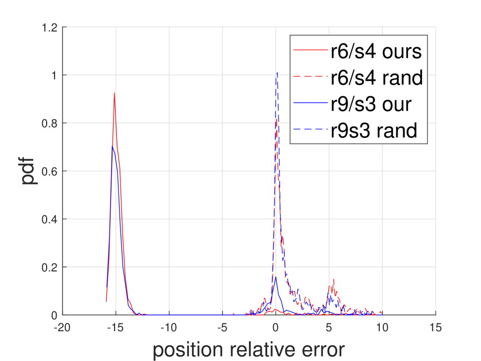
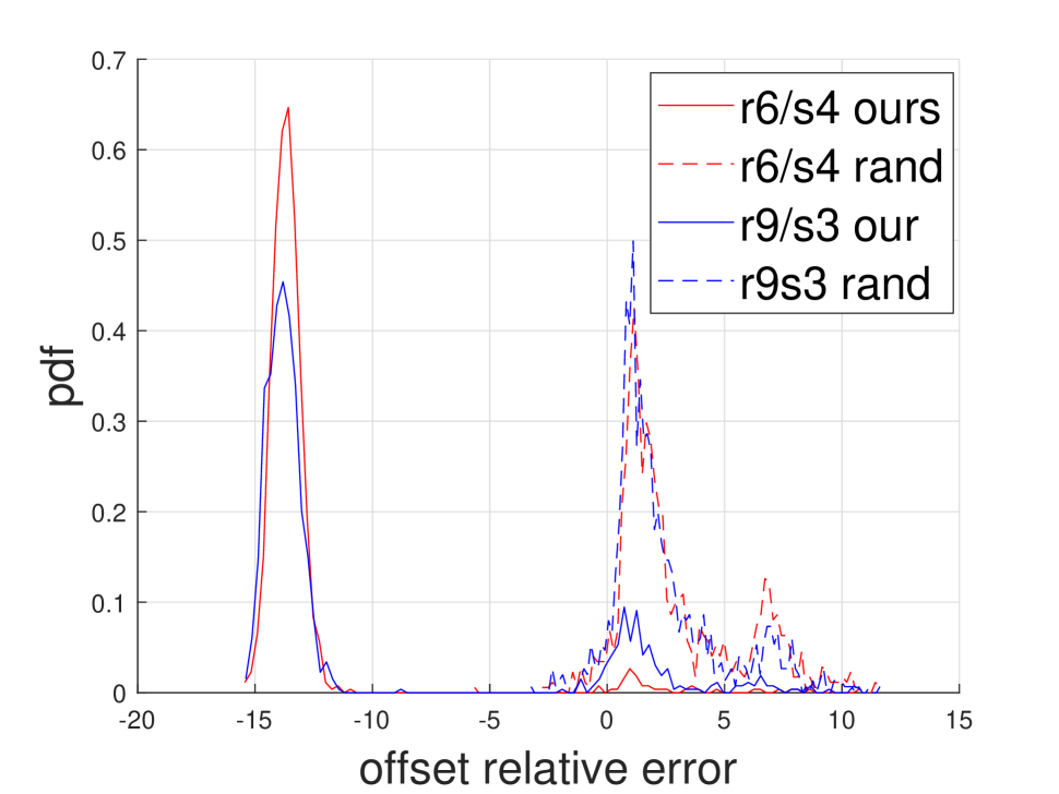
To evaluate our solvers, we randomly generate input data and solve the self-calibration problem using our proposed solvers. At this step, we consider noiseless data. We also compare our solvers with the situation where the iterative algorithm is initialized with random positions and offsets, drawn from the same distributions of the ground truths. The relative error distributions, obtained running the solvers 1000 times with different random data, are shown in Fig. 1 and the median relative errors in Table 4. As can be noticed, even for clean data, a random initialization fails to converge. Our solver on the other side, produces accurate solutions, with the relative error being practically equal to the machine epsilon of the computer. Furthermore, using the solution of our solver as a starting point, the iterative algorithm converges already after very few iterations.
| Solver | Position error () | Offset Error () |
|---|---|---|
| 9r/3s rand | 0.31 | 1.63 |
| 9r/3s our | -15 | -14 |
| 6r/4s rand | 0.55 | 1.93 |
| 6r/4s ours | -15 | -14 |
4.2 Noisy data
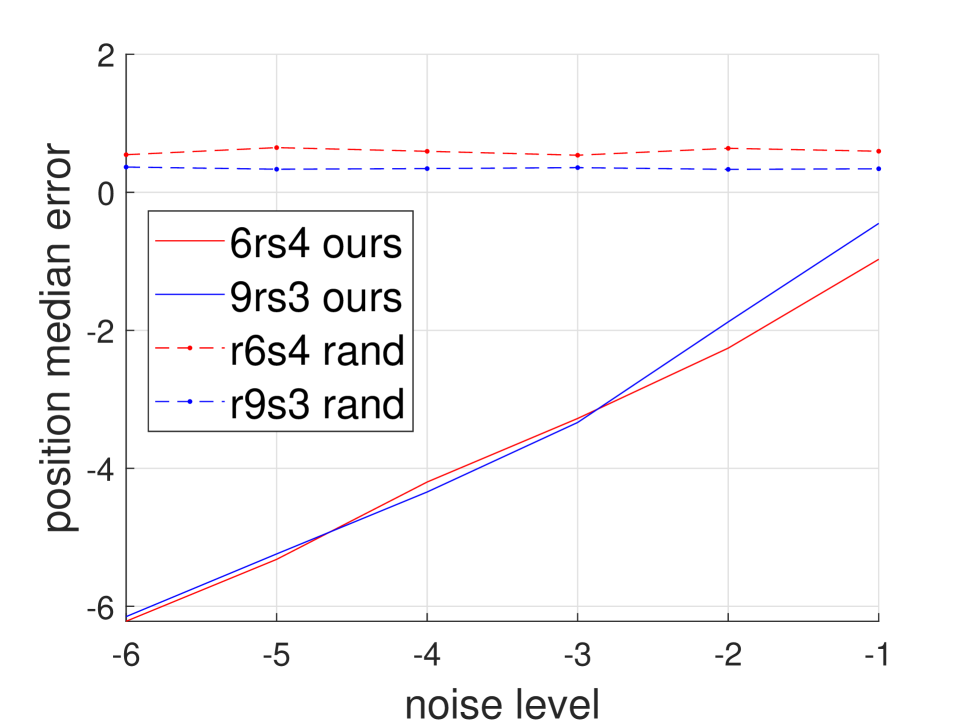
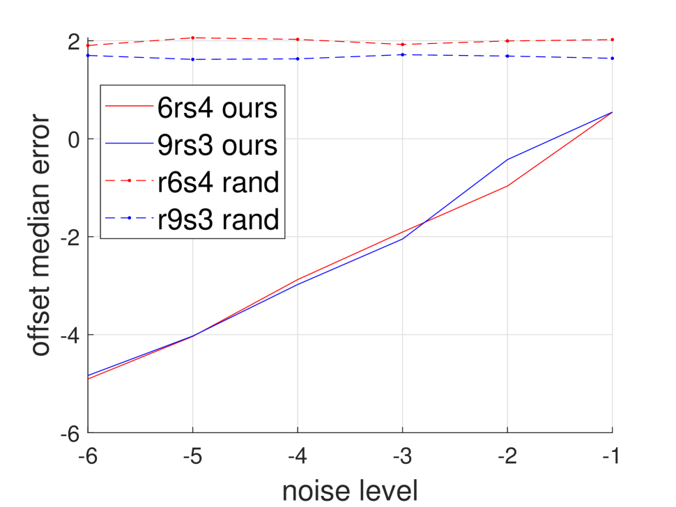
We also investigate how our solvers perform with noisy data, adding zero-mean Gaussian noise with varying standard deviation to the measurements . The results of the simulation are shown in Fig. 2. As it was discussed before, TDOA problems are sensitive to the choice of the initial value and a poor initialization can cause convergence issues. While random initialization fails, using our solvers removes this problem, allowing fast and accurate convergence, even at higher noise levels.
5 Conclusions
In this paper we considered the sensor network self-calibration problem from 2D TDOA measurements. We proposed a novel algorithm which led to new robust and efficient polynomial solvers, which allowed to solve two previously unsolved configurations. We showed that the solutions obtained with our approach are stable both for clean and noisy data.
Acknowledgments
This work was partially funded by the Academy of Finland project 327912 REPEAT.
References
- [1] K. Batstone, M. Oskarsson, and K. Åström, “Robust time-of-arrival self calibration and indoor localization using wi-fi round-trip time measurements,” in 2016 IEEE International Conference on Communications Workshops (ICC), 2016.
- [2] R. Biswas and S. Thrun, “A passive approach to sensor network localization,” in 2004 IEEE/RSJ International Conference on Intelligent Robots and Systems (IROS), 2004, pp. 1544–1549 vol.2.
- [3] D. Cox, J. Little, and D. O’Shea, Using Algebraic Geometry. Springer Verlag, 1998.
- [4] M. Crocco, A. Del Bue, and V. Murino, “A bilinear approach to the position self-calibration of multiple sensors,” IEEE Transactions on Signal Processing, pp. 660–673, 2012.
- [5] Y. Kuang, S. Burgess, A. Torstensson, and K. Åström, “A complete characterization and solution to the microphone position self-calibration problem,” in 2013 IEEE International Conference on Acoustics, Speech and Signal Processing, 2013.
- [6] Y. Kuang and K. Åström, “Stratified sensor network self-calibration from TDOA measurements,” in 21st European Signal Processing Conference (EUSIPCO 2013), 2013.
- [7] Z. Kukelova, M. Bujnak, and T. Pajdla, “Automatic generator of minimal problem solvers,” in IEEE European Conference on Computer Vision (ECCV), D. Forsyth, P. Torr, and A. Zisserman, Eds., 2008.
- [8] V. Larsson, K. Åström, and M. Oskarsson, “Efficient solvers for minimal problems by syzygy-based reduction,” Computer Vision and Pattern Recognition (CVPR), pp. 2383–2392, July 2017.
- [9] E. Miluzzo, N. D. Lane, A. T. Campbell, and R. Olfati-Saber, “Calibree: A self-calibration system for mobile sensor networks,” in Distributed Computing in Sensor Systems. Springer Berlin Heidelberg, 2008.
- [10] M. Müller, J. Lategahn, L. Telle, and C. Röhrig, “Automatic anchor calibration in IEEE 802.15.4a networks,” in 2011 8th Workshop on Positioning, Navigation and Communication, 2011.
- [11] H. Ochiai, P. Mitran, H. V. Poor, and V. Tarokh, “Collaborative beamforming for distributed wireless ad hoc sensor networks,” IEEE Transactions on Signal Processing, vol. 53, no. 11, pp. 4110–4124, 2005.
- [12] A. Plinge, F. Jacob, R. Haeb-Umbach, and G. A. Fink, “Acoustic microphone geometry calibration: An overview and experimental evaluation of state-of-the-art algorithms,” IEEE Signal Processing Magazine, vol. 33, no. 4, pp. 14–29, 2016.
- [13] M. Pollefeys and D. Nister, “Direct computation of sound and microphone locations from time-difference-of-arrival data,” in 2008 IEEE International Conference on Acoustics, Speech and Signal Processing, 2008.
- [14] N. A. B. Priyantha, H. Balakrishnan, E. D. Demaine, and S. J. Teller, “Anchor-free distributed localization in sensor networks,” in Proceedings of the 1st international conference on Embedded networked sensor systems, 2003.
- [15] C. Savarese, J. M. Rabaey, and K. Langendoen, “Robust positioning algorithms for distributed ad-hoc wireless sensor networks,” in Proceedings of the General Track of the Annual Conference on USENIX Annual Technical Conference, ser. ATEC ’02. USENIX Association, 2002.
- [16] H. Stewénius, “Gröbner basis methods for minimal problems in computer vision,” Ph.D. dissertation, Lund University, APR 2005.
- [17] C. Taylor, A. Rahimi, J. Bachrach, H. Shrobe, and A. Grue, “Simultaneous localization, calibration, and tracking in an ad hoc sensor network,” in 2006 5th International Conference on Information Processing in Sensor Networks, 2006, pp. 27–33.
- [18] J. Yick, B. Mukherjee, and D. Ghosal, “Wireless sensor network survey,” Computer Networks, 2008.
