Quark spin and orbital angular momentum from proton GPDs

Abstract

We calculate the leading-twist helicity-dependent generalized parton distributions (GPDs) of the proton at finite skewness in the Nambu–Jona-Lasinio (NJL) model of quantum chromodynamics (QCD). From these (and previously calculated helicity-independent GPDs) we obtain the spin decomposition of the proton, including predictions for quark intrinsic spin and orbital angular momentum. The inclusion of multiple species of diquarks is found to have a significant effect on the flavor decomposition, and resolving the internal structure of these dynamical diquark correlations proves essential for the mechanical stability of the proton. At a scale of $Q^{2}=4\,$GeV² we find that the up and down quarks carry an intrinsic spin and orbital angular momentum of $S_{u}=0.534$, $S_{d}=-0.214$, $L_{u}=-0.189$, and $L_{d}=0.210$, whereas the gluons have a total angular momentum of $J_{g}=0.151$. The down quark is therefore found to carry almost no total angular momentum due to cancellations between spin and orbital contributions. Comparisons are made between these spin decomposition results and lattice QCD calculations.

I INTRODUCTION

How the proton’s spin is shared among its constituents is one of the most pressing open questions in hadron physics. Ever since the European Muon Collaboration found that the quarks’ intrinsic spin falls far short of saturating the proton’s total spin Ashman et al. (1988), various theoretical efforts have gone both into accounting for the remaining spin, and into exploring the theoretical foundations for decomposing the proton’s spin. For a review, see Ref. Leader and Lorcé (2014).

A prominent gauge-invariant decomposition of spin was proposed by Ji Ji (1997a) using the flavor-separated gravitational form factors:

$$J_{a}=\frac{1}{2}\Big{(}A_{a}(0)+B_{a}(0)\Big{)}\,,$$ (1)

where $a=q,g$ are the quark and gluon contributions. This allows the proton’s spin to be decomposed into total contributions from each parton type. Since the total intrinsic spin of quarks is a gauge-invariant quantity, one may decompose $J_{q}$ further into spin and orbital angular momentum, giving a proton spin decomposition:

$$\frac{1}{2}=\sum_{q}\Big{(}S_{q}+L_{q}\Big{)}+J_{g}\,.$$ (2)

This is called the Ji spin decomposition. A gauge-invariant decomposition of $J_{g}$ into intrinsic and orbital angular momentum is not possible in this framework.

While alternative spin decompositions exist, the Ji spin decomposition has the virtue of being calculable from leading-twist generalized parton distributions (GPDs) Dittes et al. (1988); Ji (1997b); Diehl (2003). In particular, polynomiality sum rules Ji (1998) relate the Mellin moments of GPDs to gravitational and axial form factors, which when evaluated at $t=0$ give access to the total and spin angular momentum of partons. The GPDs are themselves of great contemporary interest because of their relationship to spatial light cone distributions Burkardt (2003), the proton’s mass decomposition Lorcé et al. (2019); Hatta et al. (2018), and cross sections for hard exclusive reactions such as deeply virtual Compton scattering Ji (1997b); Radyushkin (1997) that can be measured at facilities such as Jefferson Lab and an Electron Ion Collider.

It is therefore important to perform calculations of the proton’s helicity-dependent and helicity-independent leading-twist GPDs within a single framework to make a unified set of predictions. It is vital that any model calculation respect the symmetries and low-energy dynamical properties of quantum chromodynamics (QCD). Accordingly, we calculate the proton’s helicity-dependent GPDs using the Nambu–Jona-Lasinio (NJL) model of QCD Vogl and Weise (1991); Klevansky (1992); Hatsuda and Kunihiro (1994), an effective field theory that preserves all the global symmetries of QCD, reproduces dynamical chiral symmetry breaking, and can simulate aspects of confinement through use of proper time regularization Ebert et al. (1996); Hellstern et al. (1997); Cloët et al. (2014). Moreover, the NJL model has previously been used to calculate the helicity-independent proton GPDs Freese and Cloët (2020), and because these calculations are symmetry-preserving the baryon number, momentum, and angular momentum sum rules are automatically satisfied, as are constraints such as polynomiality and correct support properties.

This paper is organized as follows. In Sec. II, we discuss the formalism used for calculating the helicity-dependent proton GPDs. In Sec. III, we present the results for the GPDs and for the spin decomposition they entail. Finally, in Sec. IV we present a summary and outlook.

II FORMALISM FOR CALCULATING PROTON GPDS

The formalism for calculating the proton GPDs has been laid out already in Ref. Freese and Cloët (2020). However, we briefly review the formalism here, with additional elaborations relevant to the helicity-dependent case. The proton is considered as a bound state of three dressed quarks. The bound state amplitude is found by solving the Faddeev equation, which is dominated by configurations with two of the quarks in a diquark correlation Cahill et al. (1989). In this work, we consider quark-diquark configurations specifically, in particular configurations with isoscalar, Lorentz scalar and isovector, axial vector diquarks. More information about the proton bound state amplitude can be found in Ref. Cloët et al. (2014).

The proton’s helicity-dependent GPDs are defined from the axial bilocal lightcone correlator Dittes et al. (1988); Ji (1997b); Diehl (2003):

$$A_{\lambda^{\prime}\lambda}^{q} =\bar{u}(p^{\prime},\lambda^{\prime})\Big{[}\not{n}\gamma_{5}\,\widetilde{H}^{q}(x,\xi,t)$$

$$\hskip 71.13188pt+\frac{\gamma_{5}(n\Delta)}{2M_{N}}\,\widetilde{E}^{q}(x,\xi,t)\Big{]}u(p,\lambda)\,,$$ (3)

where $P=\frac{1}{2}(p^{\prime}+p)$, $\Delta=p^{\prime}-p$, $\xi=-2(\Delta n)/(Pn)$, $t=\Delta^{2}$, and $n$ is a lightlike vector defining the light front. The GPDs are Lorentz-invariant functions of the three explicitly written Lorentz-invariant arguments, and also dependent on a renormalization scale $\mu$ not notated above. In the NJL model calculation, we take $\mu=M=400$ MeV Cloët et al. (2005a, 2008, 2014).

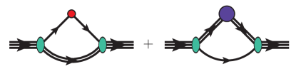
Figure 1: Diagrams contributing to the leading-twist proton GPDs. On the left is the quark diagram and on the right is the diquark diagram. The single line is the dressed quark propagator, the double line the diquark propagator, the shaded oval the Faddeev vertex, and the shaded circles represent the dressed quark and diquark GPDs.

The axial correlator itself is calculated by evaluating Feynman diagrams, with the bilocal operator defining the GPDs inserted onto either a quark within a diquark or on the accompanying quark, both scenarios being depicted diagramatically in Fig. 1. For the diquark propagators we implement the widely-used pole approximation Mineo et al. (1999); Cloët et al. (2005b); Eichmann et al. (2008); Nicmorus et al. (2009); Matevosyan et al. (2012); Roberts et al. (2011); Wilson et al. (2012); Segovia et al. (2014); Carrillo-Serrano et al. (2016). Self-consistency then demands that on-shell forms for the diquark GPDs be used Horikawa and Bentz (2005), even though they are in general off-shell. These approximations mean that the inner structures of the diquarks are folded into the proton through a convolution relation, which takes the form Freese and Cloët (2020):

$$H_{X}(x,\xi,t)=\int\frac{\mathrm{d}y}{|y|}\,h_{Y/X}(y,\xi,t)\ H_{Y}\!\left(\frac{x}{y},\frac{\xi}{y},t\right),$$ (4)

where a hadron (proton) $X$ contains a composite hadron (diquark) $Y$, and where $h_{Y/X}$ signifies “body GPDs” that encode the distribution of $Y$ within $X$. The isospin weights for the quark and diquark diagrams, for each quark flavor, are given in Eqs. (102) and (103) of Ref. Cloët et al. (2014).

II.1 Helicity-dependent diquark GPDs

We proceed to consider the helicity-dependent GPDs of diquarks. We first remark that scalar diquarks do not have helicity-dependent GPDs, since the lack of total angular momentum does not provide a quantization axis. Thus we need consider just axial vector diquarks and transition GPDs between the two diquark species.

The axial vector diquark has four helicity-dependent GPDs. We parametrize the on-shell correlator in the following way:

$$A_{a}^{q,\mu\nu} =\frac{(n\Delta)}{\Delta^{2}}\frac{i\epsilon_{\Delta\mu\nu P}}{(Pn)}\ \widetilde{H}_{1a}^{q}(x,\xi,t)$$

$$-\frac{i\epsilon_{n\Delta P\mu}\Delta^{\nu}-i\epsilon_{n\Delta P\nu}\Delta^{\mu}+i(P\Delta)\epsilon_{n\mu\nu\Delta}}{\Delta^{2}(Pn)}$$

$$\hskip 56.9055pt\times\left[-\widetilde{H}_{1a}^{q}(x,\xi,t)+\frac{\Delta^{2}}{M_{a}^{2}}\widetilde{H}_{2a}^{q}(x,\xi,t)\right]$$

$$-\frac{i\epsilon_{n\Delta P\mu}\Delta^{\nu}+i\epsilon_{n\Delta P\nu}\Delta^{\mu}}{M_{a}^{2}(Pn)}\ \widetilde{H}_{3a}^{q}(x,\xi,t)$$

$$+\frac{i\epsilon_{n\Delta P\mu}n^{\nu}+i\epsilon_{n\Delta P\nu}n^{\mu}}{2(Pn)^{2}}\ \widetilde{H}_{4a}^{q}(x,\xi,t)\,,$$ (5)

where $M_{a}$ is the axial vector diquark mass. When contracted with polarization vectors $\varepsilon_{\mu}$ and $\varepsilon^{\prime*}_{\nu}$, this is equivalent to the standard form given in Ref. Berger et al. (2001), owing to a Schouten identity and the fact that the polarization vectors are orthogonal to the diquark momenta. We choose the form in Eq. (5) in part because $\Delta$ has no virtuality dependence, thus being preferred over $P$ for having a free Lorentz index, and in part because it prevents the appearance of unphysical poles in the axial form factors. (See App. A for more details on the elimination of these unphysical poles.)

Scalar-to-axial-vector and axial-vector-to-scalar (sa and as) transition GPDs must be considered. The bilocal axial correlator for scalar-to-axial transitions is:

$$A_{sa}^{q,\nu} =\frac{n^{\nu}M_{as}}{(Pn)}\ \widetilde{H}_{sa,1}(x,\xi,t)+\frac{(n\Delta)\Delta^{\nu}}{(Pn)M_{as}}\ \widetilde{H}_{sa,2}(x,\xi,t)\,,$$ (6)

where $M_{as}=M_{s}+M_{a}$ and $M_{s}$ is the scalar diquark mass. There is an analogous expression for the axial-vector-to-scalar transition case. These GPDs have the property of being neither T-even nor T-odd. However, they remain related by time-reversal symmetry in a vital respect:

$$\widetilde{H}_{sa,i}(x,\xi,t)=-\widetilde{H}_{as,i}(x,-\xi,t)\,.$$ (7)

Crucially, the proton body GPDs accompanying these diquark GPDs in the convolution formula Eq. (4) exhibit this same property, which ensures that any T-odd contributions to the proton GPDs resulting from the diquark transition diagrams cancel out—a necessity, since proton GPDs are strictly T-even.

II.2 Dressed quark GPDs

The dressed quarks in the NJL model are quasi-particles arising from an amalgamation of nearly massless current quarks. Since GPDs are defined using bilocal operators of current quark fields, the dressed quarks have nontrivial GPDs that must be calculated within the NJL model and folded into hadrons via Eq. (4). As discussed in Ref. Freese and Cloët (2020), the leading-twist dressed quark GPDs can be obtained by solving an inhomogeneous Bethe-Salpeter equation. For the helicity-dependent GPDs, one has $\not{n}\gamma_{5}\delta(n[xP-k])$ as a driving term.

We find the isoscalar and isovector helicity-dependent dressed quark GPDs to be:

$$\widetilde{H}_{I=0,1}(x,\xi,t) =\delta(1-x)\,,$$ (8a)

$$\widetilde{E}_{I=0,1}(x,\xi,t) =\frac{N_{c}}{2\pi^{2}}\frac{1}{|\xi|}\frac{G_{\eta,\pi}M^{2}}{1+2G_{\eta,\pi}\Pi_{PP}(t)}$$

$$\times\Gamma\left(0,\alpha/\Lambda_{\mathrm{UV}}^{2},\alpha/\Lambda_{\mathrm{IR}}^{2}\right)\ \Theta(|\xi|-|x|)\,,$$ (8b)

where $\Gamma(s,a,b)=\int_{a}^{b}\mathrm{d}t\,t^{s-1}\,e^{-t}$ is the generalized incomplete gamma function and $\alpha=M^{2}-\frac{1}{4}(1-x^{2}/\xi^{2})t$. We remark that the support region for the dressing functions [i.e., for the contributions to the GPDs other than $\delta(1-x)$] is entirely constrained to the ERBL region, and thus that the PDF in particular is undressed. It’s also worth noting that the GPD $\widetilde{E}_{I}(x,\xi,t)$ contains a pion pole or $\eta$ meson pole, depending on the isospin.

III RESULTS

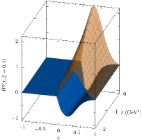
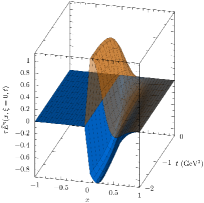
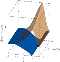
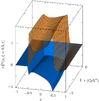
Figure 2: The helicity-dependent proton GPDs at the model scale of $Q^{2}=0.16\,$GeV², where the GPD $\widetilde{E}^{q}(x,\xi,t)$ has been scaled by a factor $\tau=-t/(4M_{N}^{2})$. The top row is for $\xi=0$ and the bottom row has $\xi=0.5$. The transparent (orange) surface is up quarks and the opaque (blue) surface is down quarks.

With the formalism above, we proceed to present results for the helicity-dependent GPDs of the proton, as well as for the proton spin decomposition. Specifically, the model parameters from Ref. Cloët et al. (2014) are used. However, in addition, we also consider a model variant with only scalar diquarks. For this, the scalar diquark parameter $G_{s}$ is found by solving proton’s Faddeev equation with the proton mass fixed to its physical value. In the scalar-only model, we find $G_{s}=9.98$ GeV^-2 and $M_{s}=576$ MeV.

III.1 Helicity-dependent proton GPDs

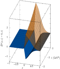
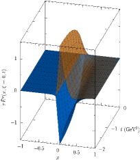
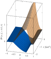
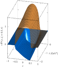
Figure 3: The helicity-dependent proton GPDs at the scale of $Q^{2}=4.0\,$GeV², where the GPD $\widetilde{E}^{q}(x,\xi,t)$ has been scaled by a factor $\tau=-t/(4M_{N}^{2})$. The top row is for $\xi=0$ and the bottom row has $\xi=0.5$. The transparent (orange) surface is up quarks and the opaque (blue) surface is down quarks.

Helicity-dependent GPDs are presented for zero and finite skewness ($\xi=0.5$) at the model scale $Q^{2}=M^{2}$ in Fig. 2. Since the helicity-dependent GPD $\widetilde{E}^{q}(x,\xi,t)$ becomes large near $t=0$ due to the presence of a pion pole, it is scaled by a factor $\tau=-t/(4M_{N}^{2})$. We see that for $\xi=0$ our GPD results have no support for $-1<x<0$ because, at the model scale, we have not included anti-quarks in the model calculation. However, at finite skewness an ERBL region ($-\xi<x<\xi$) develops and our GPDs are non-zero in the range $-\xi<x<1$, even in this valence quark picture at the model scale. These results clearly show that GPDs at finite skewness can display radically different features from those at $\xi=0$.

Table 1: Decomposition of static properties of the proton by the various diagrammatic contributions, where the full scalar+axial diquark model is used. The quantities are given at the model scale of $Q^{2}=0.16\,$GeV² and the diquark in the brackets is the spectator.

Diagram	$\kappa_{u}$	$\kappa_{d}$	$A_{u}(0)$	$A_{d}(0)$	$B_{u}(0)$	$B_{d}(0)$	$C_{u}(0)$	$C_{d}(0)$	$S_{\mathrm{tot}}$	$L_{\mathrm{tot}}$	$J_{\mathrm{tot}}$	$g_{A}$
Quark (scalar)	$\phantom{-}1.134$	$0$	$0.248$	$0$	$\phantom{-}0.306$	$0$	$\phantom{-}0.020$	$0$	$\phantom{-}0.287$	$-0.100$	$\phantom{-}0.277$	$0.574$
Scalar diquark	$-0.546$	$-0.546$	$0.220$	$0.220$	$-0.153$	$-0.153$	$-0.516$	$-0.516$	$0$	$\phantom{-}0.068$	$\phantom{-}0.068$	$0$
Quark (axial)	$-0.150$	$-0.300$	$0.034$	$0.067$	$-0.060$	$-0.120$	$\phantom{-}0.039$	$\phantom{-}0.048$	$-0.066$	$\phantom{-}0.026$	$-0.040$	$0.044$
Axial diquark	$\phantom{-}0.785$	$\phantom{-}0.157$	$0.176$	$0.035$	$\phantom{-}0.150$	$\phantom{-}0.030$	$-0.155$	$-0.031$	$\phantom{-}0.137$	$\phantom{-}0.058$	$\phantom{-}0.195$	$0.182$
Transition diquark	$\phantom{-}0.346$	$-0.346$	$0$	$0$	$\phantom{-}0.108$	$-0.108$	$\phantom{-}0.014$	$-0.014$	$0$	$0$	$0$	$0.751$
Sum	$\phantom{-}1.569$	$-1.045$	$0.678$	$0.322$	$\phantom{-}0.351$	$-0.351$	$-0.598$	$-0.483$	$\phantom{-}0.358$	$\phantom{-}0.142$	$\phantom{-}0.500$	$1.551$

A visually significant aspect of the $\widetilde{E}^{q}(x,\xi,t)$ results in Fig. 2 is the jump discontinuities at $x=\pm\xi$. This occurs in effective theories with a four-fermion interaction vertex Petrov et al. (1998); Polyakov and Weiss (1999); Theussl et al. (2004), and can be seen in the dressed quark GPD of Eq. (8). On the surface this is an apparent problem for QCD factorization, which requires GPDs to be continuous across the DGLAP-ERBL boundary. However, these jump discontinuities are removed by GPD evolution, rendering the model calculations compatible with QCD factorization above the model scale and allowing Compton form factors to be rigorously calculated.

In Fig. 3, we present the same helicity-dependent proton GPDs as in Fig. 2, but evolved to a scale $Q^{2}=4\,$GeV² using leading-order kernels Ji (1997b); Radyushkin (1997); Vinnikov (2006). We find that the QCD evolution has a dramatic impact on $\widetilde{E}^{q}(x,\xi,t)$, which is now also continuous across the DGLAP-ERBL boundary.

With both the helicity-dependent proton GPDs above and the previously calculated helicity-independent GPDs Freese and Cloët (2020) in hand, we will proceed to consider various static properties of the proton, with a special focus on its spin decomposition.

III.2 Static properties of the proton

Various static properties of the proton can be obtained from Mellin moments of the GPDs at $t=0$. Several of these, such as the electric charge, magnetic moment, axial charge, and quark spin $S_{q}$ can be obtained from form factors and have been studied elsewhere (see Ref. Cloët et al. (2014) for electromagnetic properties). Others, such as the total angular momentum $J$, the anomalous gravitomagnetic moment $B(0)$, and the D-term $C(0)$ are new opportunities afforded through GPDs. The gravitational form factors $A(t)$, $B(t)$, and $C(t)$ can be obtained from the helicity-independent GPDs through:

$$\sum_{a=q,g}\int_{-1}^{1}\mathrm{d}x\,xH^{a}(x,\xi,t) =A(t)+\xi^{2}C(t)$$ (9)

$$\sum_{a=q,g}\int_{-1}^{1}\mathrm{d}x\,xE^{a}(x,\xi,t) =B(t)-\xi^{2}C(t)\,,$$ (10)

and the total angular momentum can then be obtained through the Ji sum rule in Eq. (1). Moreover, by not summing over parton flavors, one can obtain a flavor decomposition of these quantities, although such a breakdown will be renormalization scheme and scale dependent (unlike the sum, which is scheme and scale independent).

The quark spin can be obtained from the helicity-dependent GPDs:

$$S_{q}=\frac{1}{2}\int_{-1}^{1}\mathrm{d}x\,\widetilde{H}^{q}(x,\xi,t=0)\,,$$ (11)

and the quark orbital angular momentum can then be obtained through $L_{q}=J_{q}-S_{q}$. The isovector axial vector charge $g_{A}$ is related to the up and down intrinsic spin via the Bjorken sum rule: $g_{A}=2(S_{u}-S_{d})$.

We present the results for various static quantities of the proton, along with a diagram-by-diagram breakdown, in Tab. 1. In particular, these quantities are calculated with both scalar and axial vector diquarks present in the proton. The first two columns of results provide contributions to the proton’s flavor-separated anomalous magnetic moment, which are included to provide a comparison with other results and because they would vanish in the absence of orbital angular momentum in the proton. The next two columns provide quark momentum factors in the proton, and we find that scalar diquark configurations carry about twice the light-cone momentum as the axial vector configurations. In addition, up quarks carry about two-thirds and down quarks about one-third of the total light-cone momentum, as naively expected.

For the flavor separated quantities in Tab. 1 we first remark that not only does the total $B(0)$ vanish (as expected by angular momentum conservation) but that the total contribution from each diquark configuration also vanishes. However, this is not the case for $B_{u}(0)$ or $B_{d}(0)$ separately. This is a similar observation to that found in Ref. Brodsky et al. (2001), where each state in a Fock space expansion has $B(0)=0$, and has the same formal cause: the diquark configuration (or the Fock state) has the same quantum numbers as the proton, and is thus a $J=\frac{1}{2}$ eigenstate. Thus we can say $\langle J\rangle=\frac{1}{2}\langle x\rangle=\frac{1}{2}A(0)$ for each configuration (or Fock state) individually, entailing $B(0)=0$.

We next remark on the $C(0)$ contributions of the various diagrams. The negativity condition Perevalova et al. (2016), which states that $C(0)<0$ is necessary for mechanical stability, is satisfied by both diquark configurations. In both cases, $C(0)$ is positive for the quark diagram and negative for the diquark diagram. This illustrates the necessity of resolving the dynamical diquark degrees of freedom in order to obtain a mechanically stable proton.

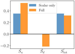
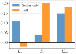
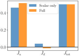
Figure 4: Spin decomposition at the model scale. The scalar diquark only model variant is contrasted with the full model containing both scalar and axial vector diquarks.

For the total intrinsic spin contribution $S_{\rm tot}=S_{u}+S_{d}$ we find that scalar diquark configurations dominate, even though the scalar diquark itself has no intrinsic spin. For $L_{\rm tot}$ and $J_{\rm tot}$ the situation is more subtle because of cancellations between different contributions. However, we note that diquark transition diagrams cannot contribute to conserved quantum numbers, since the scalar and axial vector diquark configurations are effectively orthogonal states. Moreover, the transition diagrams cannot contribute to any isoscalar quantities such as $S$, $L$, or $C(0)$ because the transition itself is isovector (namely, from an isovector to an isoscalar diquark, or vice-versa). On the other hand, they can make a potentially large contribution to isovector quantities such as $S_{u}-S_{d}$. In fact, the transition diagram is responsible for nearly half of our calculated value for $g_{A}$. In this case, one can see that $g_{A}$ is an overestimate compared to the experimental value of $g_{A}=1.2732(23)$ Tanabashi et al. (2018). This discrepancy can be alleviated by the inclusion of meson cloud effects, as done in Ref. Cloët et al. (2014) for the simpler calculations of proton electromagnetic form factors.

III.3 Proton spin decomposition

The leading-twist proton GPDs allow us to obtain the Ji decomposition of proton spin. In particular, the quark total angular momentum $J_{q}$ can be broken up into $S_{q}$ and $L_{q}$, and the total gluon angular momentum $J_{g}$ can be obtained at an evolved scale from the perturbatively generated gluon GPDs. Since the Ji decomposition does not allow $J_{g}$ to be broken into spin and orbital components, we will use $S_{\mathrm{tot}}$ and $L_{\mathrm{tot}}$ to signify the total quark spin and orbital angular momentum.

In Fig. 4, we compare the proton spin decomposition at the model scale for both variants of our NJL model, that is, one where the proton has only scalar diquark correlations and the full model that also includes axial vector diquarks. Remarkably, the total angular momentum carried by each quark flavor, as well as the total quark spin and total quark orbital angular momentum change very little when axial vector diquarks are introduced. This may be attributed to the static approximation is used for the quark-diquark interaction kernel, where orbital angular momentum is generated by relativistic effects, in particular, by the presence of a p-wave component in the quark wave function Thomas (2008). Since the relativistic effects are about equally strong in both variants of the model, $L_{\mathrm{tot}}$ and $S_{\mathrm{tot}}$ are about equal.

In the scalar-only model, $S_{d}=0$ because the down quark is present only in the diquark, which does not allow a spin quantization axis to be identified. Non-relativistically, one would have $L_{d}=J_{d}=0$ as well, but the remaining quark in the proton carrying orbital angular momentum—since it can exist in a p-wave state—implies that the diquark, and thus the down quark, can carry orbital angular momentum as well. The diagram breakdown for the full model in Tab. 2 indeed shows that $L_{d}$ and $J_{d}$ are non-zero because of the scalar diquark diagram.

The flavor breakdown of $J$, $L$, and $S$ changes significantly when axial vector diquarks are present, for two reasons. The first—but more minor—reason is that the flavor breakdown within axial diquark configurations differs from the scalar diquark case. The effects of this are minimal however, and owe entirely to relativistic effects. Non-relativistically (and within the static approximation), there is no orbital angular momentum, and the axial diquark configuration has a spin wave function: $\left|J_{p}^{z}=+\tfrac{1}{2}\right\rangle=\sqrt{\tfrac{2}{3}}\left|J^{z}_{\mathrm{dq}}=+1;J^{z}_{q}=-\tfrac{1}{2}\right>-\sqrt{\tfrac{1}{3}}\left|J^{z}_{\mathrm{dq}}=0;J^{z}_{q}=+\tfrac{1}{2}\right>$ which when combined with the appropriate isospin recombination coefficients, gives $J_{d}=S_{d}=0$. Indeed, even within the proper NJL model calculation, we find the contributions to $J_{d}$ and $S_{d}$ from the axial diquark diagrams are $0.006$ and $-0.021$, respectively.

Table 2: Flavor decomposition of the total, spin, and orbital angular momenta, where the results include contributions from both scalar and axial vector diquarks. Results are at the model scale of $Q^{2}=0.16$ GeV² and the diquark in the brackets is the spectator.

Diagram	$J_{u}$	$J_{d}$	$S_{u}$	$S_{d}$	$L_{u}$	$L_{d}$
Quark (scalar)	$\phantom{-}0.277$	$0$	$\phantom{-}0.287$	$0$	$-0.010$	$0$
Scalar diquark	$\phantom{-}0.034$	$\phantom{-}0.034$	$0$	$0$	$\phantom{-}0.034$	$\phantom{-}0.034$
Quark (axial)	$-0.013$	$-0.026$	$-0.022$	$-0.044$	$\phantom{-}0.009$	$\phantom{-}0.018$
Axial diquark	$\phantom{-}0.163$	$\phantom{-}0.033$	$\phantom{-}0.114$	$\phantom{-}0.023$	$\phantom{-}0.049$	$\phantom{-}0.010$
Transition diquark	$\phantom{-}0.054$	$-0.054$	$\phantom{-}0.188$	$-0.188$	$-0.134$	$\phantom{-}0.134$
Sum	$\phantom{-}0.514$	$-0.014$	$\phantom{-}0.567$	$-0.209$	$-0.053$	$\phantom{-}0.195$

The most significant contributions to the change in flavor breakdown come from transition diagrams. Although $J$ is a conserved quantity, individual flavor contributions are not. Moreover, individual flavor contributions are not isoscalar, and in fact $J_{u}-J_{d}$ etc. are isovector, meaning the transition diagram has the potential to make significant changes to these differences. In fact, as can be seen in Tab. 2, $S_{d}$ and $L_{d}$ are dominated by the transition diagram, although this diagram makes a small contribution to $J_{d}$.

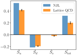
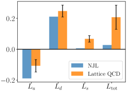
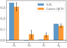
Figure 5: Comparison of NJL model spin decomposition to the lattice QCD results of Ref. Alexandrou et al. (2017) at $Q^{2}=4$ GeV². The NJL results contain contributions from both scalar and axial vector diquarks.

Overall, $J_{d}$ comes out very close to zero in the scalar+axial model. This can be seen as arising from cancellations. On one hand, $S_{d}$ and $L_{d}$ end up being nearly equal and opposite after contributions from all the diagrams have been summed. On the other hand, in Tab. 1 one sees that $A_{d}(0)$ and $B_{d}(0)$ are nearly equal and opposite after summing the diagrams.

Besides inter-model comparisons, it is worth comparing our flavor-separated proton spin decomposition to the best available estimates for the true proton spin decomposition. Although experimental extractions for linear combinations of $J_{u}$ and $J_{d}$ exist from JLab Mazouz et al. (2007) and HERMES Ye (2006); Airapetian et al. (2008), these extractions are model-dependent and may not be instructive. On the other hand, there exists a lattice QCD computation of the proton spin decomposition at physical pion mass Alexandrou et al. (2017).

In Fig. 5, we compare our results (with both diquark species present) to the lattice results of Ref. Alexandrou et al. (2017) at a scale of $Q^{2}=4$ GeV². One can observe mixed agreement with the lattice results. Firstly, it’s worth remarking that the broad qualitative agreement on the sign and magnitude of $J_{u}$, $J_{d}$, $L_{u}$, $L_{d}$, $S_{u}$, and $S_{d}$ is remarkable considering the simplicity and minimalism of the NJL model. This is suggestive that the spin decomposition of the proton is governed to a large extent by three effects: its diquark content, relativistic effects that can generate $L$, and QCD evolution (which connects the model scale to the empirical scale). Further intricacies (such as a meson cloud) could be somewhat large but seem to be second-order effects. Solving the Faddeev equation beyond the static approximation will also have an impact, however since the spin decomposition is defined through $t=0$ moments, the effects of exchange diagrams are expected to be small.

The agreement for $J_{g}$ is surprising, since in our calculation this is generated purely by QCD evolution, and is therefore suggestive of a small intrinsic gluon angular momentum. Our calculations also tend to overestimate $S_{q}$ for the light quarks, which could be rectified by the inclusion of a pion and kaon cloud, which would also generate the missing intrinsic $S_{s}$ contributions. Since $J_{q}$ agrees reasonably well with lattice, corrections that decrease $S_{q}$ would at the same time need to increase $L_{q}$, which is natural in the meson cloud picture because of their p-wave couplings to the quarks or nucleon.

IV SUMMARY AND OUTLOOK

In this work, we calculated the helicity-dependent and helicity-independent leading-twist proton GPDs in a confining version of the NJL model. A quark-diquark approximation was used for the proton, and two variants of the model were considered: (1) a model with only isoscalar, Lorentz scalar diquarks; and (2) a model also containing isovector, axial vector diquarks. In both model variants, a flavor-separated spin decomposition was performed for the proton, and the presence of both diquark species was found to contribute significantly to the flavor-separated spin decomposition, but little to $S_{\mathrm{tot}}$ and $L_{\mathrm{tot}}$. In particular, transition diagrams between the diquark species—which can affect only isoscalar quantities, such as $S_{u}-S_{d}$—was responsible for most of the difference between the models’ spin decompositions.

The model variant with both diquarks present was found to have mixed agreement with lattice results for the proton’s spin decomposition. The discrepancies are due primarily to the NJL model’s overestimates of spin and underestimates of orbital angular momentum, along with the lack of strangeness content. The former of these discrepancies can be resolved by the inclusion of a pion cloud, and the latter with the inclusion of a kaon cloud. These improvements warrant future work on the subject.

Appendix A Longitudinal-transverse separation for axial operators

The non-local operator defining the helicity-dependent GPDs, as well as the local axial current, are defined using matrix elements of the operator $\bar{q}(x)\gamma_{\mu}\gamma_{5}q(y)$, with the spacetime points $x$ and $y$ determined by the application in question. This operator notoriously does not correspond to a conserved current. However, it is possible to break the operator into a “transverse” piece that is conserved and a “longitudinal” piece that is not. The breakdown is most clear in momentum space, where we define:

$$(\gamma_{\mu}\gamma_{5})_{\perp}=\left(\gamma_{\mu}-\frac{\Delta_{\mu}\not{\Delta}}{\Delta^{2}}\right)\gamma_{5}\,,\qquad(\gamma_{\mu}\gamma_{5})_{\parallel}=\frac{\Delta_{\mu}\not{\Delta}}{\Delta^{2}}\gamma_{5}\,,$$ (12)

with $\Delta$ being the momentum transfer to the target. That $(\gamma_{\mu}\gamma_{5})_{\perp}$ is transverse to $\Delta$ makes $\bar{q}(x)(\gamma_{\mu}\gamma_{5})_{\perp}q(x)$ a conserved local current.

Notably, the dynamics of $\bar{q}(x)(\gamma_{\mu}\gamma_{5})_{\perp}q(y)$ and $\bar{q}(x)(\gamma_{\mu}\gamma_{5})_{\parallel}q(y)$ completely decouple. This means that the Bethe-Salpeter equations for the local currents $\bar{q}(0)(\gamma_{\mu}\gamma_{5})_{\perp}q(0)$ and $\bar{q}(0)(\gamma_{\mu}\gamma_{5})_{\parallel}q(0)$ decouple from each other, and also that the BSEs for the leading-twist non-local correlators

$$A_{\perp,\parallel}^{q}=\frac{1}{2}\int\frac{\mathrm{d}z}{2\pi}e^{ix(Pn)\kappa}$$

$$\hskip 8.53581pt\times\left\langle p^{\prime}\lambda^{\prime}\middle|\bar{q}\left(-\frac{nz}{2}\right)(\not{n}\gamma_{5})_{\perp,\parallel}\left[-\frac{nz}{2},\frac{nz}{2}\right]q\left(\frac{nz}{2}\right)\middle|p\lambda\right\rangle,$$ (13)

decouple from each other.

The Lorentz decompositions of the transverse and longitudinal components of the helicity-dependent correlator can be written, for a spin-half particle, as:

$$A_{\perp,\lambda^{\prime}\lambda}^{q} =\bar{u}(p^{\prime},\lambda^{\prime})(\not{n}\gamma_{5})_{\perp}u(p,\lambda)\,\widetilde{H}(x,\xi,t),$$ (14)

$$A_{\parallel,\lambda^{\prime}\lambda}^{q} =\bar{u}(p^{\prime},\lambda^{\prime})(\not{n}\gamma_{5})_{\parallel}u(p,\lambda)\,\left[\widetilde{H}(x,\xi,t)-\tau\widetilde{E}(x,\xi,t)\right]$$

$$\equiv\bar{u}(p^{\prime},\lambda^{\prime})(\not{n}\gamma_{5})_{\parallel}u(p,\lambda)\,\widetilde{E}_{\parallel}(x,\xi,t)\,.$$ (15)

Comparing to Eq. (8), we observe that the pion pole can contribute only to the longitudinal component of the correlator. This additionally means that the pion pole will not be present in $\widetilde{H}^{q}(x,\xi,t)$—nor $G_{A}(t)$—of the proton.

For an on-shell spin-one particle, the longitudinal-transverse separation can be written:

$$A_{\perp,\lambda^{\prime}\lambda}^{q} =-i\Bigg{(}\frac{\epsilon_{n\Delta P\rho}}{\Delta^{2}}\frac{\varepsilon^{\rho}(\varepsilon^{\prime*}\Delta)-\varepsilon^{\prime*\rho}(\varepsilon\Delta)}{(Pn)}$$

$$\hskip 48.36967pt+\frac{(P\Delta)}{\Delta^{2}}\frac{\epsilon_{n\varepsilon\varepsilon^{\prime*}\Delta}}{(Pn)}\Bigg{)}\left[-\widetilde{H}_{1}^{q}+\frac{\Delta^{2}}{M_{a}^{2}}\widetilde{H}_{2}^{q}\right]$$

$$-\frac{i\epsilon_{n\Delta P\rho}}{M_{a}^{2}}\frac{\varepsilon^{\rho}(\varepsilon^{\prime*}\Delta)+\varepsilon^{\prime*\rho}(\varepsilon\Delta)}{(Pn)}\,\widetilde{H}_{3}^{q}$$

$$+\frac{i\epsilon_{n\Delta P\rho}}{2(Pn)}\frac{\varepsilon^{\rho}(\varepsilon^{\prime*}n)+\varepsilon^{\prime*\rho}(\varepsilon n)}{(Pn)}\,\widetilde{H}_{4}^{q},$$ (16a)

$$A_{\parallel,\lambda^{\prime}\lambda}^{q} =\frac{(n\Delta)}{\Delta^{2}}\frac{i\epsilon^{\Delta\varepsilon\varepsilon^{\prime*}P}}{(Pn)}\,\widetilde{H}_{1}^{q}\,.$$ (16b)

This breakdown agrees exactly with the standard breakdown in Ref. Berger et al. (2001) for on-shell particles, through use of the Schouten identity result:

$$(n \Delta)\epsilon^{\Delta\varepsilon\varepsilon^{\prime*}P}=\Delta^{2}\epsilon^{n\varepsilon\varepsilon^{\prime*}P}$$

$$-\epsilon^{n\Delta P\sigma}\Big{(}\varepsilon_{\sigma}(\varepsilon^{\prime*}\Delta)-\varepsilon^{\prime*}_{\sigma}(\varepsilon\Delta)\Big{)}-(\Delta P)\epsilon^{n\varepsilon\varepsilon^{\prime*}\Delta}\,,$$ (17)

and the on-shell relation $(\Delta P)=0$, as well as use of the identities $(\varepsilon\Delta)=2(\varepsilon P)$ and $(\varepsilon^{\prime*}\Delta)=-2(\varepsilon^{*}P)$.

For an off-shell particle, $(\Delta P)\neq 0$ means the equivalence between the decompositions no longer holds. Crucially, the decompositions differ by a transverse structure that multiplies a longitudinal GPD. This means using the standard decomposition for an off-shell spin-one particle will introduce unphysical pion poles into transverse quantities, such as $G_{A}(t)$ of the proton. Therefore, the alternative decomposition suggested in Eq. (16)—which indeed does not produce unphysical pion poles in the proton’s axial form factor—is preferred for the off-shell spin-one correlator.

One last crucial aspect of Eq. (16) worth remarking on is the explicit inclusion of a term proportional to $(P\Delta)$. For an on-shell spin-one particle, this term is zero and is not important. For an off-shell particle, however, it is necessary for the axial correlator $A^{q}_{\lambda^{\prime}\lambda}$ to be analytic at $t=0$. Neither the Lorentz structure multiplying $\widetilde{H}^{q}_{1}$ in Eq. (16b) nor the structure multiplying $-\widetilde{H}_{1}^{q}+\frac{t}{M_{a}^{2}}\,\widetilde{H}_{2}^{q}$ in Eq. (16a) has a well-defined forward limit; if one writes $\Delta^{\mu}=\sqrt{-t}\,e^{\mu}$, with $e^{\mu}$ an arbitrary spacelike unit vector, then the $t\rightarrow 0^{-}$ limit depends on $e^{\mu}$, which is unphysical. However, by virtue of the Schouten identity Eq. (17) and the presence of the $(P\Delta)$ term in Eq. (16a), the total axial correlator $A^{q}_{\parallel,\lambda^{\prime}\lambda}+A^{q}_{\perp,\lambda^{\prime}\lambda}$ does have a well-defined $t=0$ limit, even when $(P\Delta)\neq 0$.

References

- Ashman et al. (1988) J. Ashman et al. (European Muon), Phys. Lett. B 206, 364 (1988).
- Leader and Lorcé (2014) E. Leader and C. Lorcé, Phys. Rept. 541, 163 (2014), arXiv:1309.4235 [hep-ph] .
- Ji (1997a) X.-D. Ji, Phys. Rev. Lett. 78, 610 (1997a), arXiv:hep-ph/9603249 [hep-ph] .
- Dittes et al. (1988) F. M. Dittes, D. Mueller, D. Robaschik, B. Geyer, and J. Horejsi, Phys. Lett. B209, 325 (1988).
- Ji (1997b) X.-D. Ji, Phys. Rev. D55, 7114 (1997b), arXiv:hep-ph/9609381 [hep-ph] .
- Diehl (2003) M. Diehl, Phys. Rept. 388, 41 (2003), arXiv:hep-ph/0307382 [hep-ph] .
- Ji (1998) X.-D. Ji, J. Phys. G24, 1181 (1998), arXiv:hep-ph/9807358 [hep-ph] .
- Burkardt (2003) M. Burkardt, Int. J. Mod. Phys. A18, 173 (2003), arXiv:hep-ph/0207047 [hep-ph] .
- Lorcé et al. (2019) C. Lorcé, H. Moutarde, and A. P. Trawiński, Eur. Phys. J. C79, 89 (2019), arXiv:1810.09837 [hep-ph] .
- Hatta et al. (2018) Y. Hatta, A. Rajan, and K. Tanaka, JHEP 12, 008 (2018), arXiv:1810.05116 [hep-ph] .
- Radyushkin (1997) A. V. Radyushkin, Phys. Rev. D56, 5524 (1997), arXiv:hep-ph/9704207 [hep-ph] .
- Vogl and Weise (1991) U. Vogl and W. Weise, Prog. Part. Nucl. Phys. 27, 195 (1991).
- Klevansky (1992) S. P. Klevansky, Rev. Mod. Phys. 64, 649 (1992).
- Hatsuda and Kunihiro (1994) T. Hatsuda and T. Kunihiro, Phys. Rept. 247, 221 (1994), arXiv:hep-ph/9401310 [hep-ph] .
- Ebert et al. (1996) D. Ebert, T. Feldmann, and H. Reinhardt, Phys. Lett. B388, 154 (1996), arXiv:hep-ph/9608223 [hep-ph] .
- Hellstern et al. (1997) G. Hellstern, R. Alkofer, and H. Reinhardt, Nucl. Phys. A625, 697 (1997), arXiv:hep-ph/9706551 [hep-ph] .
- Cloët et al. (2014) I. C. Cloët, W. Bentz, and A. W. Thomas, Phys. Rev. C90, 045202 (2014), arXiv:1405.5542 [nucl-th] .
- Freese and Cloët (2020) A. Freese and I. C. Cloët, Phys. Rev. C 101, 035203 (2020), arXiv:1907.08256 [nucl-th] .
- Cahill et al. (1989) R. T. Cahill, C. D. Roberts, and J. Praschifka, Austral. J. Phys. 42, 129 (1989).
- Cloët et al. (2005a) I. C. Cloët, W. Bentz, and A. W. Thomas, Phys. Lett. B621, 246 (2005a), arXiv:hep-ph/0504229 [hep-ph] .
- Cloët et al. (2008) I. C. Cloët, W. Bentz, and A. W. Thomas, Phys. Lett. B659, 214 (2008), arXiv:0708.3246 [hep-ph] .
- Mineo et al. (1999) H. Mineo, W. Bentz, and K. Yazaki, Phys. Rev. C60, 065201 (1999), arXiv:nucl-th/9907043 [nucl-th] .
- Cloët et al. (2005b) I. C. Cloët, W. Bentz, and A. W. Thomas, Phys. Rev. Lett. 95, 052302 (2005b), arXiv:nucl-th/0504019 [nucl-th] .
- Eichmann et al. (2008) G. Eichmann, A. Krassnigg, M. Schwinzerl, and R. Alkofer, Annals Phys. 323, 2505 (2008), arXiv:0712.2666 [hep-ph] .
- Nicmorus et al. (2009) D. Nicmorus, G. Eichmann, A. Krassnigg, and R. Alkofer, Phys. Rev. D80, 054028 (2009), arXiv:0812.1665 [hep-ph] .
- Matevosyan et al. (2012) H. H. Matevosyan, W. Bentz, I. C. Cloët, and A. W. Thomas, Phys. Rev. D85, 014021 (2012), arXiv:1111.1740 [hep-ph] .
- Roberts et al. (2011) H. L. L. Roberts, L. Chang, I. C. Cloët, and C. D. Roberts, Few Body Syst. 51, 1 (2011), arXiv:1101.4244 [nucl-th] .
- Wilson et al. (2012) D. J. Wilson, I. C. Cloët, L. Chang, and C. D. Roberts, Phys. Rev. C85, 025205 (2012), arXiv:1112.2212 [nucl-th] .
- Segovia et al. (2014) J. Segovia, C. Chen, I. C. Cloët, C. D. Roberts, S. M. Schmidt, and S. Wan, Few Body Syst. 55, 1 (2014), arXiv:1308.5225 [nucl-th] .
- Carrillo-Serrano et al. (2016) M. E. Carrillo-Serrano, W. Bentz, I. C. Cloët, and A. W. Thomas, Phys. Lett. B759, 178 (2016), arXiv:1603.02741 [nucl-th] .
- Horikawa and Bentz (2005) T. Horikawa and W. Bentz, Nucl. Phys. A 762, 102 (2005), arXiv:0506021 [nucl-th] .
- Berger et al. (2001) E. R. Berger, F. Cano, M. Diehl, and B. Pire, Phys. Rev. Lett. 87, 142302 (2001), arXiv:hep-ph/0106192 [hep-ph] .
- Petrov et al. (1998) V. Yu. Petrov, P. V. Pobylitsa, M. V. Polyakov, I. Bornig, K. Goeke, and C. Weiss, Phys. Rev. D57, 4325 (1998), arXiv:hep-ph/9710270 [hep-ph] .
- Polyakov and Weiss (1999) M. V. Polyakov and C. Weiss, Phys. Rev. D60, 114017 (1999), arXiv:hep-ph/9902451 [hep-ph] .
- Theussl et al. (2004) L. Theussl, S. Noguera, and V. Vento, Eur. Phys. J. A20, 483 (2004), arXiv:nucl-th/0211036 [nucl-th] .
- Vinnikov (2006) A. V. Vinnikov, (2006), arXiv:hep-ph/0604248 [hep-ph] .
- Brodsky et al. (2001) S. J. Brodsky, D. S. Hwang, B.-Q. Ma, and I. Schmidt, Nucl. Phys. B593, 311 (2001), arXiv:hep-th/0003082 [hep-th] .
- Perevalova et al. (2016) I. A. Perevalova, M. V. Polyakov, and P. Schweitzer, Phys. Rev. D94, 054024 (2016), arXiv:1607.07008 [hep-ph] .
- Tanabashi et al. (2018) M. Tanabashi et al. (Particle Data Group), Phys. Rev. D 98, 030001 (2018).
- Thomas (2008) A. W. Thomas, Phys. Rev. Lett. 101, 102003 (2008), arXiv:0803.2775 [hep-ph] .
- Alexandrou et al. (2017) C. Alexandrou, M. Constantinou, K. Hadjiyiannakou, K. Jansen, C. Kallidonis, G. Koutsou, A. Vaquero Avilés-Casco, and C. Wiese, Phys. Rev. Lett. 119, 142002 (2017), arXiv:1706.02973 [hep-lat] .
- Mazouz et al. (2007) M. Mazouz et al. (Jefferson Lab Hall A), Phys. Rev. Lett. 99, 242501 (2007), arXiv:0709.0450 [nucl-ex] .
- Ye (2006) Z. Ye (HERMES), in Deep inelastic scattering. Proceedings, 14th International Workshop, DIS 2006, Tsukuba, Japan, April 20-24, 2006 (2006) pp. 679–682, arXiv:hep-ex/0606061 [hep-ex] .
- Airapetian et al. (2008) A. Airapetian et al. (HERMES), JHEP 06, 066 (2008), arXiv:0802.2499 [hep-ex] .