Muonium-antimuonium oscillations in effective field theory

Abstract

Flavor violating processes in the lepton sector have highly suppressed branching ratios in the standard model mainly due to the tiny neutrino mass. This means that observing lepton flavor violation (LFV) in the next round of experiments would constitute a clear indication of physics beyond the standard model (BSM). We revisit a discussion of one possible way to search for LFV, muonium-antimuonium oscillations. This process violates muon lepton number by two units and could be sensitive to the types of BSM physics that are not probed by other types of LFV processes. Using techniques of effective field theory, we calculate the mass and width differences of the mass eigenstates of muonium. We argue that its invisible decays give the parametrically leading contribution to the lifetime difference and put constraints on the scales of new physics probed by effective operators in muonium oscillations.

I Introduction

Flavor-changing neutral current (FCNC) interactions serve as a powerful probe of physics beyond the standard model (BSM). Since no local operators generate FCNCs in the standard model (SM) at tree level, new physics (NP) degrees of freedom can effectively compete with the SM particles running in the loop graphs, making their discovery possible. This is, of course, only true provided the BSM models include flavor-violating interactions.

An especially clean system to study BSM effects in lepton sector is muonium ${M_{\mu}}$, a QED bound state of a positively-charged muon and a negatively-charged electron, $|{M_{\mu}}\rangle\equiv|\mu^{+}e^{-}\rangle$. The main decay channel for both states is driven by the weak decay of the muon. The average lifetime of a muonium state $\tau_{M_{\mu}}$ is expected to be the same as that of the muon, $\tau_{\mu}=(2.1969811\pm 0.0000022)\times 10^{-6}$ s Tanabashi:2018oca , apart from the tiny effect due to time dilation, $(\tau_{M_{\mu}}-\tau_{\mu})/\tau_{\mu}=\alpha^{2}m_{e}^{2}/(2m_{\mu}^{2})=6\times 10^{-10}$ Czarnecki:1999yj . Just like a positronium or a Hydrogen atom, muonium could be produced in two spin configurations, a spin-one triplet state called ortho-muonium, and a spin-zero singlet state called para-muonium. We shall denote the para-muonium state as $\left|{M_{\mu}^{P}}\right\rangle$ and the ortho-muonium state as $\left|{M_{\mu}^{V}}\right\rangle$. If the spin of the state does not matter, we shall employ the notation $\left|{M_{\mu}}\right\rangle$.

So far, we have not yet observed FCNC in the charged lepton sector. This is because in the standard model with massive neutrinos the charged lepton flavor violating (CLFV) transitions are suppressed by the powers of $m^{2}_{\nu}/m^{2}_{W}$, which renders the predictions for their transition rates vanishingly small, e.g. ${\cal B}(\mu\to e\gamma)_{\nu SM}\sim 10^{-54}$ Raidal:2008jk ; Bernstein:2013hba . Yet, experimental analyses constantly push the bounds on the CLFV transitions. It might be that in some models of NP, such as a model with the doubly-charged Higgs particles Swartz:1989qz ; Chang:1989uk ; Kiers:2005gh ; Kiers:2005vx , the effective $\Delta L=2$ transitions could occur at a rate that is not far below the sensitivity of currently-operating experiments. Alternatively, it might be that no term that changes the lepton flavor by two units is present in a BSM Lagrangian. But even in this case, a subsequent application of two $\Delta L=1$ interactions would also generate an effective $\Delta L=2$ interaction.

Such a $\Delta L=2$ interaction would then change the muonium state into the anti-muonium one, leading to the possibility of muonium-anti-muonium oscillations. As a variety of well-established new physics models contain $\Delta L=2$ interaction terms Raidal:2008jk , observation of muonium converting into anti-muonium could then provide especially clean probes of new physics in the leptonic sector Bernstein:2013hba ; Willmann:1998gd . Theoretical analyses of conversion probability for such transitions have been actively studied, mainly using the framework of particular models Pontecorvo:1957cp ; Feinberg:1961zza ; ClarkLove:2004 ; CDKK:2005 ; Li:2019xvv ; Endo:2020mev . It would be useful to perform a model-independent computation of the oscillation parameters using techniques of effective theory that includes all possible BSM models encoded in a few Wilson coefficients of effective operators. We do so in this paper, computing all relevant QED matrix elements. Finally, employing similar effective field theory (EFT) techniques for computation of the contributions that are non-local at the muon mass scale, we present them in terms of the series of local operators expanded in inverse powers of $m_{\mu}$ Beneke:1996gn ; Golowich:2005pt .

In this paper we discuss the most general analysis of $M_{\mu}-\overline{M}_{\mu}$ oscillations in the framework of effective field theory. We review phenomenology of muonium oscillations in Sec. II, taking into account both mass and lifetime differences in the muonium system. We compute the mass and width differences in Sec. III. In Sec. IV we constrain the BSM scale $\Lambda$ using experimental muonium-anti-muonium oscillation parameters. We conclude in Sec. V. Appendix VI contains some details of calculations.

II Phenomenology of Muonium Oscillations

Phenomenology of $M_{\mu}-\overline{M}_{\mu}$ oscillations is very similar to phenomenology of meson-antimeson oscillations Donoghue ; Nierste . There are, however, several important differences that we will emphasize below. One major difference is related to the fact that both ortho- and para-muonium can, in principle, oscillate. While most studies only considered muonium oscillations due to the BSM heavy states, below we also discuss the possibility of oscillations via the light states. Since such states can go on mass shell, these contributions would lead to the possibility of a lifetime difference in the $M_{\mu}-\overline{M}_{\mu}$ system.

If the new physics Lagrangian includes lepton-flavor violating interactions, the time development of a muonium and anti-muonium states would be coupled, so it would be appropriate to consider their combined evolution,

$$|\psi(t)\rangle=\left({\begin{array}[]{c}a(t)\\ b(t)\\ \end{array}}\right)=a(t)|{M_{\mu}}\rangle+b(t)|\overline{M_{\mu}}\rangle.$$ (1)

The time evolution of $|\psi(t)\rangle$ evolution is governed by a Schrödinger equation,

$$i\frac{d}{dt}\begin{pmatrix}\left|M_{\mu}(t)\right\rangle\\ \left|\overline{M}_{\mu}(t)\right\rangle\end{pmatrix}=\left(m-i\frac{\Gamma}{2}\right)\begin{pmatrix}\left|M_{\mu}(t)\right\rangle\\ \left|\overline{M}_{\mu}(t)\right\rangle\end{pmatrix}.$$ (2)

CPT-invariance dictates that the masses and widths of muonium and anti-muonium are the same, $m_{11}=m_{22}$, $\Gamma_{11}=\Gamma_{22}$, while CP-invariance of the $\Delta L_{\mu}=2$ interaction, which we assume for simplicity, dictates that

$$m_{12}=m^{*}_{21},\qquad\Gamma_{12}=\Gamma^{*}_{21}.$$ (3)

The presence of off-diagonal pieces in the mass matrix signals that it needs to be diagonalized. The mass eigenstates $|{M_{\mu}}_{1,2}\rangle$ can be defined as

$$|{M_{\mu}}_{1,2}\rangle=\frac{1}{\sqrt{2}}\left[|{M_{\mu}}\rangle\mp|{\overline{M}_{\mu}}\rangle\right],$$ (4)

where we neglected CP-violation and employed a convention where $CP|{M_{\mu}}_{\pm}\rangle=\mp|{M_{\mu}}_{\pm}\rangle$. The mass and the width differences of the mass eigenstates are

$$\Delta m\equiv M_{1}-M_{2},\qquad\Delta\Gamma\equiv\Gamma_{2}-\Gamma_{1}.$$ (5)

where $M_{i}$ ($\Gamma_{i}$) are the masses (widths) of the mass eigenstates $|{M_{\mu}}_{1,2}\rangle$. We defined $\Delta m$ and $\Delta\Gamma$ to be either positive or negative, which is to be determined by experiment. It is often convenient to introduce dimensionless quantities,

$$x=\frac{\Delta m}{\Gamma},\qquad y=\frac{\Delta\Gamma}{2\Gamma},$$ (6)

where the average lifetime $\Gamma=(\Gamma_{1}+\Gamma_{2})/2$. It is important to note that while $\Gamma$ is defined by the standard model decay rate of the muon, $x$ and $y$ are driven by the lepton-flavor violating interactions. It is then expected that both $x,y\ll 1$.

The time evolution of flavor eigenstates follows from Eq. (2) Donoghue ; Nierste ,

$$\left|M(t)\right\rangle = g_{+}(t)\left|{M_{\mu}}\right\rangle+g_{-}(t)\left|{\overline{M}_{\mu}}\right\rangle,$$

$$\left|\overline{M}(t)\right\rangle = g_{-}(t)\left|{M_{\mu}}\right\rangle+g_{+}(t)\left|{\overline{M}_{\mu}}\right\rangle,$$ (7)

where the coefficients $g_{\pm}(t)$ are defined as

$$g_{\pm}(t)=\frac{1}{2}e^{-\Gamma_{1}t/2}e^{-iM_{1}t}\left[1\pm e^{\Delta\Gamma t/2}e^{i\Delta mt}\right].$$ (8)

As $x,y\ll 1$ we can expand Eq. (8) to get

$$g_{+}(t) = e^{-\Gamma_{1}t/2}e^{-iM_{1}t}\left[1+\frac{1}{8}\left(y-ix\right)^{2}\left(\Gamma t\right)^{2}\right],$$

$$g_{-}(t) = \frac{1}{2}e^{-\Gamma_{1}t/2}e^{-iM_{1}t}\left(y-ix\right)\left(\Gamma t\right).$$ (9)

Denoting an amplitude for the muonium decay into a final state $f$ as $A_{f}=\langle f|{\cal H}|{M_{\mu}}\rangle$ and an amplitude for its decay into a CP-conjugated final state $\overline{f}$ as $A_{\bar{f}}=\langle\overline{f}|{\cal H}|{M_{\mu}}\rangle$, we can write the time-dependent decay rate of ${M_{\mu}}$ into the $\overline{f}$,

$$\Gamma({M_{\mu}}\to\overline{f})(t)=\frac{1}{2}N_{f}\left|A_{f}\right|^{2}e^{-\Gamma t}\left(\Gamma t\right)^{2}R_{M}(x,y),$$ (10)

where $N_{f}$ is a phase-space factor and $R_{M}(x,y)$ is the oscillation rate,

$$R_{M}(x,y)=\frac{1}{2}\left(x^{2}+y^{2}\right).$$ (11)

Integrating over time and normalizing to $\Gamma({M_{\mu}}\to f)$ we get the probability of ${M_{\mu}}$ decaying as ${\overline{M}_{\mu}}$ at some time $t>0$,

$$P({M_{\mu}}\rightarrow{\overline{M}_{\mu}})=\frac{\Gamma({M_{\mu}}\to\overline{f})}{\Gamma({M_{\mu}}\to f)}=R_{M}(x,y).$$ (12)

This equation generalizes oscillation probability computed in the classic papers Feinberg:1961zza ; CDKK:2005 by accounting for the lifetime difference in the muonium system, making it dependent on both the normalized mass $x$ and the lifetime $y$ differences. We will compute those in the next section.

We shall use the data from the most recent experiment Willmann:1998gd in order to place constraints on the oscillation parameters. To do so, we have to account for the fact that the set-up described in Willmann:1998gd had muonia propagating in a magnetic field $B_{0}$. This magnetic field suppresses oscillations by removing degeneracy between ${M_{\mu}}$ and ${\overline{M}_{\mu}}$. It also has a different effect on different spin configurations of the muonium state and the Lorentz structure of the operators that generate mixing Cuypers:1996ia ; Horikawa:1995ae . Experimentally these effects were accounted for by introducing a factor $S_{B}(B_{0})$. The oscillation probability is then Willmann:1998gd ,

$$P({M_{\mu}}\rightarrow{\overline{M}_{\mu}})\leq 8.3\times 10^{-11}/S_{B}(B_{0}).$$ (13)

We shall use different values of $S_{B}(B_{0})$, presented in Table II of Willmann:1998gd when placing constraints on the Wilson coefficients of effective operators in the next section.

III Effective Theory of Oscillations

Muonium-anti-muonium oscillations could be effective probes of flavor-violating new physics in leptons. One of the issues is that at this point we do not know which particular model of new physics will provide the correct ultraviolet (UV) extension for the standard model. However, since the muonium mass is most likely much smaller than the new particle masses, it is not necessary to know it. Any new physics scenario which involves lepton flavor violating interactions can be matched to an effective Lagrangian, ${\cal L}_{\rm eff}$, whose Wilson coefficients would be determined by the UV physics that becomes active at some scale $\Lambda$ Grzadkowski:2010es ; Petrov:2016azi ,

$${\cal L}_{\rm eff}=-\frac{1}{\Lambda^{2}}\underset{i}{\sum}c_{i}(\mu)Q_{i},$$ (14)

where the $c_{i}$’s are the short distance Wilson coefficients. They encode all model-specific information. $Q_{i}$’s are the effective operators which reflect degrees of freedom relevant at the scale at which a given process takes place. If we assume that no new light particles (such as “dark photons” or axions) exist in the low energy spectrum, those operators would be written entirely in terms of the SM degrees of freedom. In the case at hand, all SM particles with masses larger than that of the muon should also be integrated out, leaving only muon, electron, photon, and neutrino degrees of freedom.

It would be convenient for us to classify effective operators in Eq. (14) by their lepton quantum numbers. In particular, we can write the effective Lagrangian as

$${\cal L}_{\rm eff}={\cal L}_{\rm eff}^{\Delta L_{\mu}=0}+{\cal L}_{\rm eff}^{\Delta L_{\mu}=1}+{\cal L}_{\rm eff}^{\Delta L_{\mu}=2}$$ (15)

The first term in this expansion contains both the standard model and the new physics contributions. It then follows that the leading term in ${\cal L}_{\rm eff}^{\Delta L_{\mu}=0}$ is suppressed by powers of $M_{W}$, not the new physics scale $\Lambda$. We should emphasize that only the operators that are local at the scale of the muonium mass are retained in Eq. (15).

The second term contains $\Delta L_{\mu}=1$ operators. As we integrated out all heavy degrees of freedom, the operators of lowest possible dimension that governs muonium oscillations must be of dimension six. The most general dimension six effective Lagrangian, $\mathcal{L}_{\rm eff}^{\Delta L_{\mu}=1}$, has the form Celis:2014asa ; Hazard:2017udp

$${\cal L}_{\rm eff}^{\Delta L_{\mu}=1}= - \frac{1}{\Lambda^{2}}\sum_{f}\Big{[}\left(C_{VR}^{f}\ \overline{\mu}_{R}\gamma^{\alpha}e_{R}+C_{VL}^{f}\ \overline{\mu}_{L}\gamma^{\alpha}e_{L}\right)\ \overline{f}\gamma_{\alpha}f$$

$$+ \ \left(C_{AR}^{f}\ \overline{\mu}_{R}\gamma^{\alpha}e_{R}+C_{AL}^{q}\ \overline{\mu}_{L}\gamma^{\alpha}e_{L}\right)\ \overline{f}\gamma_{\alpha}\gamma_{5}f$$

$$+ \ m_{e}m_{f}G_{F}\left(C_{SR}^{f}\ \overline{\mu}_{R}e_{L}+C_{SL}^{f}\ \overline{\mu}_{L}e_{R}\right)\ \overline{f}f$$

$$+ \ m_{e}m_{f}G_{F}\left(C_{PR}^{f}\ \overline{\mu}_{R}e_{L}+C_{PL}^{f}\ \overline{\mu}_{L}e_{R}\right)\ \overline{f}\gamma_{5}f$$

$$+ \ m_{e}m_{f}G_{F}\left(C_{TR}^{f}\ \overline{\mu}_{R}\sigma^{\alpha\beta}e_{L}+C_{TL}^{f}\ \overline{\mu}_{L}\sigma^{\alpha\beta}e_{R}\right)\ \overline{f}\sigma_{\alpha\beta}f+h.c.~{}\Big{]},$$

where $G_{F}\sim M_{W}^{-2}$ is the Fermi constant, $\mu$ and $e$ are the fermion fields, $(\mu,e)_{L,R}=P_{L,R}(\mu,e)$. $P_{R,L}=\frac{1}{2}\left(1\pm\gamma^{5}\right)$ are the projection operators, and $f$ represents other fermions that are not integrated out at the the muonium scale. The subscripts on the Wilson coefficients are for the type of Lorentz structure: vector, axial-vector, scalar, pseudo-scalar, and tensor. The Wilson coefficients would in general be different for different fermions $f$. Note that the Lagrangian Eq. (III) also contains terms that do not follow from the dimension six in the standard model effective field theory (SMEFT), but could be generated by higher order operators. This is taken into account by introducing mass and $G_{F}$ factors emulating such suppression Celis:2014asa ; Hazard:2017udp .

The last term in Eq. (15), ${\cal L}_{\rm eff}^{\Delta L_{\mu}=2}$, represents the effective operators changing the lepton quantum number by two units. The leading contribution to muonium oscillations is given by the dimension six operators. The most general effective Lagrangian

$${\cal L}_{\rm eff}^{\Delta L_{\mu}=2}=-\frac{1}{\Lambda^{2}}\underset{i}{\sum}C^{\Delta L=2}_{i}(\mu)Q_{i}(\mu).$$ (17)

can be written with the operators written entirely in terms of the muon and electron degrees of freedom,

$$Q_{1} = \left(\overline{\mu}_{L}\gamma_{\alpha}e_{L}\right)\left(\overline{\mu}_{L}\gamma^{\alpha}e_{L}\right),\quad Q_{2}=\left(\overline{\mu}_{R}\gamma_{\alpha}e_{R}\right)\left(\overline{\mu}_{R}\gamma^{\alpha}e_{R}\right),$$

$$Q_{3} = \left(\overline{\mu}_{L}\gamma_{\alpha}e_{L}\right)\left(\overline{\mu}_{R}\gamma^{\alpha}e_{R}\right),\quad Q_{4}=\left(\overline{\mu}_{L}e_{R}\right)\left(\overline{\mu}_{L}e_{R}\right),$$

$$Q_{5} = \left(\overline{\mu}_{R}e_{L}\right)\left(\overline{\mu}_{R}e_{L}\right).$$ (18)

We did not include operators that could be related to the presented ones via Fierz relations. It is important to note that some of the operators in Eq. (III) are not invariant under the SM gauge group $SU(2)_{L}\times U(1)$. This means that they receive additional suppression, as they may be generated from the higher-dimensional operators in SMEFT Petrov:2016azi .

Other $\Delta L_{\mu}=2$ local operators that will be important later in this paper can be written as

$$Q_{6}=\left(\overline{\mu}_{L}\gamma_{\alpha}e_{L}\right)\left(\overline{\nu_{\mu}}_{L}\gamma^{\alpha}{\nu_{e}}_{L}\right),\quad Q_{7}=\left(\overline{\mu}_{R}\gamma_{\alpha}e_{R}\right)\left(\overline{\nu_{\mu}}_{L}\gamma^{\alpha}{\nu_{e}}_{L}\right),$$ (19)

where we only included SMEFT operators that contain left-handed neutrinos Petrov:2016azi ; Grossman:2003rw . In order to see how these operators (and thus new physics) contribute to the mixing parameters, it is instructive to consider off-diagonal terms in the mass matrix Donoghue

$$\left(m-\frac{i}{2}\Gamma\right)_{12}=\frac{1}{2M_{M}}\left\langle{\overline{M}_{\mu}}\left|{\cal H}_{\rm eff}\right|{M_{\mu}}\right\rangle+\frac{1}{2M_{M}}\sum_{n}\frac{\left\langle{\overline{M}_{\mu}}\left|{\cal H}_{\rm eff}\right|n\right\rangle\left\langle n\left|{\cal H}_{\rm eff}\right|{M_{\mu}}\right\rangle}{M_{M}-E_{n}+i\epsilon},$$ (20)

where the first term does not contain imaginary part, so it contributes to $m_{12}$, i.e. the mass difference. The second term contains bi-local contributions connected by physical intermediate states. This term has both real and imaginary parts and thus contributes to both $m_{12}$ and $\Gamma_{12}$.

III.1 Mass difference: $\Delta L_{\mu}=2$ operators

We can rewrite Eq.(20) to extract the physical mixing parameters $x$ and $y$ of Eq. (6). For the mass difference,

$$x=\frac{1}{2M_{M}\Gamma}\mbox{Re}\left[2\langle{\overline{M}_{\mu}}\left|{\cal H}_{\rm eff}\right|{M_{\mu}}\rangle+\langle{\overline{M}_{\mu}}\left|i\int d^{4}x\ \mbox{T}\left[{\cal H}_{\rm eff}(x){\cal H}_{\rm eff}(0)\right]\right|{M_{\mu}}\rangle\right]$$ (21)

Assuming the LFV NP is present, the dominant local contribution to $x$ comes from the last term in Eq. (15),

$$\langle{\overline{M}_{\mu}}|{\cal H}_{\rm eff}|{M_{\mu}}\rangle=\langle{\overline{M}_{\mu}}|{\cal H}_{\rm eff}^{\Delta L_{\mu}=2}|{M_{\mu}}\rangle$$ (22)

provided that only $Q_{1}-Q_{5}$ operators are taken into account. It is easy to see that the relevant contributions are only suppressed by $\Lambda^{2}$. Other contributions, including the non-local double insertions of ${\cal L}_{\rm eff}^{\Delta L_{\mu}=1}$, represented by the second term in Eq. (21), do contribute to the mass difference, but are naively suppressed by $\Lambda^{4}$. Thus, we shall not consider them in this paper.

In order to evaluate the mass difference contribution, we need to take the matrix elements. As explained in the Introduction, we expect that both spin-0 singlet and spin-1 triplet muonium states would undergo oscillations. The oscillation parameters would in general be different, as the matrix elements would differ for those two cases.

Using factorization approach familiar from the meson flavor oscillation, the matrix elements can be easily written in terms of the muonium decay constant $f_{M}$ Hazard:2016fnc ; Fael:2018 .

$$\left\langle 0\right|\overline{\mu}\gamma^{\alpha}\gamma^{5}e\left|{M_{\mu}^{P}}\right\rangle = if_{P}p^{\alpha},\quad\left\langle 0\right|\overline{\mu}\gamma^{\alpha}e\left|{M_{\mu}^{V}}\right\rangle=f_{V}M_{M}\epsilon^{\alpha}(p),$$

$$\left\langle 0\right|\overline{\mu}\sigma^{\alpha\beta}e\left|{M_{\mu}^{V}}\right\rangle = if_{T}\left(\epsilon^{\alpha}p^{\beta}-\epsilon^{\beta}p^{\alpha}\right),$$ (23)

where $p^{\alpha}$ is para-muonium’s four-momentum, and $\epsilon^{\alpha}(p)$ is the ortho-muonium’s polarization vector. Note that $f_{P}=f_{V}=f_{T}=f_{M}$ in the non-relativistic limit. The decay constant can be written in terms of the bound-state wave function,

$$f_{M}^{2}=4\frac{\left|\varphi(0)\right|^{2}}{M_{M}},$$ (24)

which is the QED’s version of Van Royen-Weisskopf formula. For a Coulombic bound state the wave function of the ground state is

$$\varphi(r)=\frac{1}{\sqrt{\pi a_{\tiny{M_{\mu}}}^{3}}}e^{-\frac{r}{a_{\tiny{M_{\mu}}}}},$$ (25)

where $a_{\tiny{M_{\mu}}}=(\alpha m_{\rm red})^{-1}$ is the muonium Bohr radius, $\alpha$ is the fine structure constant, and $m_{red}=m_{e}m_{\mu}/(m_{e}+m_{\mu})$ is the reduced mass. Then,

$$|\varphi(0)|^{2}=\frac{(m_{red}\alpha)^{3}}{\pi}=\frac{1}{\pi}(m_{red}\alpha)^{3}.$$ (26)

In the non-relativistic limit factorization gives the exact result for the QED matrix elements of the six-fermion operators. Nevertheless, we explicitly verified that this is indeed the case (see Appendix VI).

Para-muonium. The matrix elements of the spin-singlet states can be obtained from Eq. (III) using the definitions of Eq. (III.1),

$$\left\langle{\bar{M}_{\mu}^{P}}\right|Q_{1}\left|{M_{\mu}^{P}}\right\rangle = \ \ f_{M}^{2}M_{M}^{2},\ \quad\left\langle{\bar{M}_{\mu}^{P}}\right|Q_{2}\left|{M_{\mu}^{P}}\right\rangle=\ \ f_{M}^{2}M_{M}^{2},$$

$$\left\langle{\bar{M}_{\mu}^{P}}\right|Q_{3}\left|{M_{\mu}^{P}}\right\rangle = -\frac{3}{2}f_{M}^{2}M_{M}^{2},\quad\left\langle{\bar{M}_{\mu}^{P}}\right|Q_{4}\left|{M_{\mu}^{P}}\right\rangle=-\frac{1}{4}f_{M}^{2}M_{M}^{2},$$

$$\left\langle{\bar{M}_{\mu}^{P}}\right|Q_{5}\left|{M_{\mu}^{P}}\right\rangle = -\frac{1}{4}f_{M}^{2}M_{M}^{2}.$$ (27)

Combining the contributions from the different operators and using the definitions from Eqs. (24) and (26), we obtain an expression for $x_{P}$ for the para-muonium state,

$$x_{P}=\frac{4(m_{red}\alpha)^{3}}{\pi\Lambda^{2}\Gamma}\left[C_{1}^{\Delta L=2}+C_{2}^{\Delta L=2}-\frac{3}{2}C_{3}^{\Delta L=2}-\frac{1}{4}\left(C_{4}^{\Delta L=2}+C_{5}^{\Delta L=2}\right)\right].$$ (28)

This result is universal and holds true for any new physics model that can be matched into a set of local $\Delta L=2$ interactions.

Ortho-muonium. Using the same procedure, but computing the relevant matrix elements for the vector ortho-muonium state, we obtain the matrix elements

$$\left\langle{\bar{M}_{\mu}^{V}}\right|Q_{1}\left|{M_{\mu}^{V}}\right\rangle = -3f_{M}^{2}M_{M}^{2},\quad\left\langle{\bar{M}_{\mu}^{V}}\right|Q_{2}\left|{M_{\mu}^{V}}\right\rangle=-3f_{M}^{2}M_{M}^{2},$$

$$\left\langle{\bar{M}_{\mu}^{V}}\right|Q_{3}\left|{M_{\mu}^{V}}\right\rangle = -\frac{3}{2}f_{M}^{2}M_{M}^{2},\quad\left\langle{\bar{M}_{\mu}^{V}}\right|Q_{4}\left|{M_{\mu}^{V}}\right\rangle=-\frac{3}{4}f_{M}^{2}M_{M}^{2},$$

$$\left\langle{\bar{M}_{\mu}^{V}}\right|Q_{5}\left|{M_{\mu}^{V}}\right\rangle = -\frac{3}{4}f_{M}^{2}M_{M}^{2}.$$ (29)

Again, combining the contributions from the different operators, we obtain an expression for $x_{V}$ for the ortho-muonium state,

$$x_{V}=-\frac{12(m_{red}\alpha)^{3}}{\pi\Lambda^{2}\Gamma}\left[C_{1}^{\Delta L=2}+C_{2}^{\Delta L=2}+\frac{1}{2}C_{3}^{\Delta L=2}+\frac{1}{4}\left(C_{4}^{\Delta L=2}+C_{5}^{\Delta L=2}\right)\right].$$ (30)

Again, this result is universal and holds true for any new physics model that can be matched into a set of local $\Delta L=2$ interactions.

It might be instructive to present an example of a BSM model that can be matched into the effective Lagrangian of Eq. (17) and can be constrained from Eqs. (III.1,III.1). Let us consider a model which contains a doubly-charged Higgs boson Swartz:1989qz ; Chang:1989uk ; Crivellin:2018ahj . Such states often appear in the context of left-right models Kiers:2005gh ; Kiers:2005vx . A coupling of the doubly charged Higgs field $\Delta^{--}$ to the lepton fields can be written as

$${\cal L}_{R}=g_{\ell\ell}\overline{\ell}_{R}\ell^{c}\Delta+H.c.,$$ (31)

where $\ell^{c}=C\overline{\ell}^{T}$ is the charge-conjugated lepton state. Integrating out the $\Delta^{--}$ field, this Lagrangian leads to the following effective Hamiltonian Swartz:1989qz ; Kiers:2005vx

$${\cal H}_{\Delta}=\frac{g_{ee}g_{\mu\mu}}{2M_{\Delta}^{2}}\left(\overline{\mu}_{R}\gamma_{\alpha}e_{R}\right)\left(\overline{\mu}_{R}\gamma^{\alpha}e_{R}\right)+H.c.,$$ (32)

below the scales associated with the doubly-charged Higgs field’s mass $M_{\Delta}$. Examining Eq. (32) we see that this Hamiltonian matches onto our operator $Q_{2}$ (see Eq. (III)) with the scale $\Lambda=M_{\Delta}$ and the corresponding Wilson coefficient $C_{2}^{\Delta L=2}=g_{ee}g_{\mu\mu}/2$.

III.2 Width difference: $\Delta L_{\mu}=2$ and $\Delta L_{\mu}=1$ operators

The lifetime difference in the muonium system can be obtained from Eq. (20) Golowich:2006gq . It comes from the physical intermediate states, which is signified by the imaginary part in Eq. (20) and reads,

$$y=\frac{1}{\Gamma}\sum_{n}\rho_{n}\left\langle{\overline{M}_{\mu}}\left|{\cal H}_{\rm eff}\right|n\right\rangle\left\langle n\left|{\cal H}_{\rm eff}\right|{M_{\mu}}\right\rangle,$$ (33)

where $\rho_{n}$ is a phase space function that corresponds to the intermediate state that is common for ${M_{\mu}}$ and ${\overline{M}_{\mu}}$. There are only two possible intermediate states that can contribute to $y$, $e^{+}e^{-}$ and $\nu\bar{\nu}$. The $e^{+}e^{-}$ intermediate state corresponds to a $\Delta L_{\mu}=1$ decay ${M_{\mu}}\to e^{+}e^{-}$, which implies that ${\cal H}_{\rm eff}={\cal H}_{\rm eff}^{\Delta L_{\mu}=1}$ in Eq. (33). According to Eq. (III), it appears that, quite generally, this contribution is suppressed by $\Lambda^{4}$, i.e. will be much smaller than $x$, irrespective of the values of the corresponding Wilson coefficients.

Another contribution comes from the $\nu\bar{\nu}$ intermediate state. This common intermediate state can be reached by the standard model tree level decay ${M_{\mu}}\to\overline{\nu_{\mu}}{\nu_{e}}$ interfering with the $\Delta L_{\mu}=2$ decay ${\overline{M}_{\mu}}\to\overline{\nu_{\mu}}\nu_{e}$. Such contribution is only suppressed by $\Lambda^{2}M_{W}^{2}$ and represents the parametrically leading contribution to $y$. We shall compute this contribution below.

Writing $y$ similarly to $x$ in Eq. (21), i.e. in terms of the correlation function, we obtain

$$y = \frac{1}{2M_{M}\Gamma}\mbox{Im}\left[\langle{\overline{M}_{\mu}}\left|i\int d^{4}x\ \mbox{T}\left[{\cal H}_{\rm eff}(x){\cal H}_{\rm eff}(0)\right]\right|{M_{\mu}}\rangle\right]$$ (34)

$$= \frac{1}{M_{M}\Gamma}\mbox{Im}\left[\langle{\overline{M}_{\mu}}\left|i\int d^{4}x\ \mbox{T}\left[{\cal H}_{\rm eff}^{\Delta L_{\mu}=2}(x){\cal H}_{\rm eff}^{\Delta L_{\mu}=0}(0)\right]\right|{M_{\mu}}\rangle\right],$$

where the ${\cal H}_{\rm eff}^{\Delta L_{\mu}=0}=-{\cal L}_{\rm eff}^{\Delta L_{\mu}=0}$ is given by the ordinary standard model Lagrangian,

$${\cal L}_{\rm eff}^{\Delta L_{\mu}=0}=-\frac{4G_{F}}{\sqrt{2}}\left(\overline{\mu}_{L}\gamma_{\alpha}e_{L}\right)\left(\overline{\nu_{e}}_{L}\gamma^{\alpha}{\nu_{\mu}}_{L}\right),$$ (35)

and ${\cal H}_{\rm eff}^{\Delta L_{\mu}=2}$ only contributes through the operators $Q_{6}$ and $Q_{7}$.

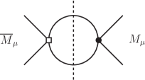
Figure 1: A contribution to $y$ described in Eq. (34). A white square represents a vertex given by Eq. (19), while a black dot is given by the SM contribution of Eq. (35). A dotted line represents the imaginary part.

Since the decaying muon injects a large momentum into the two-neutrino intermediate state, the integral in Eq. (34) is dominated by small distance contributions, compared to the scale set by $1/m_{\mu}$. We can the compute the correlation function in Eq. (34) by employing a short distance operator product expansion, systematically expanding it in powers of $1/m_{\mu}$.

$$T = i\int d^{4}x\ \mbox{T}\left[{\cal H}_{\rm eff}^{\Delta L_{\mu}=2}(x){\cal H}_{\rm eff}^{\Delta L_{\mu}=0}(0)\right]$$ (36)

$$= i\int d^{4}x\ \mbox{T}\left[\left(\overline{\mu}\Gamma_{\alpha}e\right)\left(\overline{\nu_{\mu}}_{L}\gamma^{\alpha}{\nu_{e}}_{L}\right)(x)\left(\overline{\mu}\gamma_{\beta}P_{L}e\right)\left(\overline{\nu_{e}}_{L}\gamma^{\beta}{\nu_{\mu}}_{L}\right)(0)\right],$$

The leading term is obtained by contracting the neutrino fields in Eq. (36) into propagators,

$$\contraction{}{\overline{\nu_{\mu}}}{(x)}{\nu_{\mu}}\overline{\nu}_{\mu}(x)\nu_{\mu}(0) = iS_{F}(-x),$$

$$\bcontraction{}{\nu}{{}_{e}(x)}{\overline{\nu_{e}}}\nu_{e}(x)\ \overline{\nu_{e}}(0) = iS_{F}(x),$$ (37)

where $S_{F}(x)$ represents the propagator in coordinate representation. In what follows we will consider neutrinos to be Dirac fields for simplicity.

Using Cutkoski rules to compute the discontinuity (imaginary part) of $T$ and calculating the phase space integrals we get

$$\mbox{Disc}\ T=\frac{G_{F}}{\sqrt{2}\Lambda^{2}}\frac{M_{M}^{2}}{3\pi}\left[C_{6}^{\Delta L=2}\left(Q_{1}+Q_{5}\right)+\frac{1}{2}C_{7}^{\Delta L=2}Q_{3}\right].$$ (38)

We can now compute the lifetime difference $y$ by using Eq. (34) and take the relevant matrix elements for the spin singlet and the spin triplet states of the muonium.

Para-muonium. The matrix elements of the spin-singlet state have been computed above and presented in Eq. (III.1). Computing the matrix elements in Eq. (34) using their definitions from Eqs. (24) and (26), we obtain an expression for the lifetime difference $y_{P}$ for the para-muonium state,

$$y_{P}=\frac{G_{F}}{\sqrt{2}\Lambda^{2}}\frac{M_{M}^{2}}{\pi^{2}\Gamma}(m_{red}\alpha)^{3}\left(C_{6}^{\Delta L=2}-C_{7}^{\Delta L=2}\right).$$ (39)

It is interesting to note that if $C_{6}^{\Delta L=2}=C_{7}^{\Delta L=2}$ current conservation assures that no lifetime difference is generated at this order in $1/\Lambda$ for the para-muonium.

Ortho-muonium. Similarly, using the matrix elements for the spin-triplet state computed in Eq. (III.1), the expression fo Eq. (38) leads to the lifetime difference

$$y_{V}=-\frac{G_{F}}{\sqrt{2}\Lambda^{2}}\frac{M_{M}^{2}}{\pi^{2}\Gamma}(m_{red}\alpha)^{3}\left(5C_{6}^{\Delta L=2}+C_{7}^{\Delta L=2}\right),$$ (40)

We emphasize that Eqs. (39) and (40) represent parametrically leading contributions to muonium lifetime difference, as they are only suppressed by two powers of $\Lambda$.

IV Experimental constraints

We can now use the derived expressions for $x$ and $y$ to place constraints on the BSM scale $\Lambda$ (or the Wilson coefficients $C_{i}$) from the experimental constraints on muonium-anti-muoium oscillation parameters. Since both spin-0 and spin-1 muonium states were produced in the experiment Willmann:1998gd , we should average the oscillation probability over the number of polarization degres of freedom,

$$P({M_{\mu}}\rightarrow{\overline{M}_{\mu}})_{\rm exp}=\sum_{i=P,V}\frac{1}{2S_{i}+1}P({M_{\mu}}^{i}\rightarrow{\overline{M}_{\mu}}^{i}),$$ (41)

where $P({M_{\mu}}\rightarrow{\overline{M}_{\mu}})_{\rm exp}$ is the experimental oscillation probability from Eq. (13). We shall use the values of $S_{B}(B_{0})$ for $B_{0}=2.8$ $\mu$T from the Table II of Willmann:1998gd , as it will provide us the best experimental constraints on the BSM scale $\Lambda$. We report those constraints in Table 1.

Operator	Interaction type	$~{}S_{B}(B_{0})$ (from Willmann:1998gd )	Constraints on the scale $\Lambda$, TeV
$Q_{1}$	$(V-A)\times(V-A)$	0.75	$5.4$
$Q_{2}$	$(V+A)\times(V+A)$	0.75	$5.4$
$Q_{3}$	$(V-A)\times(V+A)$	0.95	$5.4$
$Q_{4}$	$(S+P)\times(S+P)$	0.75	$2.7$
$Q_{5}$	$(S-P)\times(S-P)$	0.75	$2.7$
$Q_{6}$	$(V-A)\times(V-A)$	0.75	$0.58\times 10^{-3}$
$Q_{7}$	$(V+A)\times(V-A)$	0.95	$0.38\times 10^{-3}$

Table 1: Constraints on the energy scales probed by different $\Delta L=2$ operators of Eqs. (III) and (19). We set the corresponding Wilson coefficient $C_{i}=1$.

As one can see from Eqs. (28), (30), (39), and (40), each observable depends on the combination of the operators. We shall assume that only one operator at a time gives a dominant contribution. This ansatz is usually referred to as the single operator dominance hypothesis. It is not necessarily realized in many particular UV completions of the LFV EFTs, as cancellations among contributions of different operators are possible. It is however a useful tool in constraining parameters of ${\cal L}_{\rm eff}$.

Since it is the combination $C_{i}/\Lambda^{2}$ that enters the theoretical predictions for $x$ and $y$, one cannot separately measure $C_{i}$ and $\Lambda$. We choose to constrain the scale $\Lambda$ that is probed by the corresponding operator and set the corresponding value of the Wilson coefficient $C_{i}$ to one. Such approach, as any calculation based on effective field-theoretic techniques, has its advantages and disadvantages. The advantage of such approach is in the fact that it allows to constrain all possible models of New Physics that can generate $M_{\mu}-\overline{M}_{\mu}$ mixing. The models are encoded in the analytic expressions for the Wilson coefficients of a few effective operators in Eq. (III). The disadvantage is reflected in the fact that possible complementary studies of New Physics contributions to $\Delta L=1$ and $\Delta L=2$ processes are not straightforward. Those can be done by considering particular BSM scenarios, which is beyond the scope of this paper. The EFT techniques are then used to simplify calculations of radiative corrections.

The results are reported in Table 1. As can be seen, the experimental data provide constraints on the scales comparable to those probed by the LHC program, except for $Q_{6}$ and $Q_{7}$. The results indicate that existing bounds on $M_{\mu}-\overline{M}_{\mu}$ oscillation parameters probe NP scales of the order of several TeV. The constraints on the lepton-flavor violating neutrino operators $Q_{6}$ and $Q_{7}$ are understandably weaker, as the lifetime difference is suppressed by a factor $G_{F}/\Lambda^{2}$, while the mass difference is only suppressed by a factor of $1/\Lambda^{2}$. We would like to emphasize that constraints on the oscillation parameters come from the data that is over 20 years old Willmann:1998gd ! We find it amazing that the data obtained over two decades ago probe the same energy scales as current LHC experiments.

We urge our experimental colleagues to further study muonium-antimuonium oscillations. It would be interesting to see how far the proposed MACE experiment MACE or similar facility at FNAL could push the constraints on the muonium oscillation parameters.

V Conclusions

Lepton flavor violating transitions provide a powerful engine for new physics searches. In this work we revisited phenomenology of muonium-antimuonium oscillations. We argued that in generic models of new physics both mass and lifetime differences in the muonium system would contribute to the oscillation probability. We computed the normalized mass difference $x$ in the muonium system with the most general set of effective operators for both spin-singlet and the spin-triplet muonium states. We set up a formalism for computing the lifetime difference and computed the parametrically leading contribution to $y$. Using the derived expressions for $x$ and $y$ we then put constraints on the BSM scale $\Lambda$. From this we found that for operators $Q_{1}-Q_{5}$ the experimental data provided constraints on scales relevant to the LHC program.

VI Appendix

In this Appendix we show that the vacuum insertion approximation leads to the same answer as a direct computation of a four-fermion matrix element relevant for the muonium-anti-muonium oscillations. We shall show that by computing a matrix element of the $Q_{1}$ operator as an example. The matrix elements is defined as

$$\left\langle Q_{1}\right\rangle=\left\langle\overline{M}_{\mu}\right|\left(\overline{\mu}\gamma_{\alpha}P_{L}e\right)\left(\overline{\mu}\gamma^{\alpha}P_{L}e\right)\left|M_{\mu}\right\rangle$$ (42)

for both pseudoscalar and vector muonium states. In order to compute the matrix element in Eq. (42) we need to build the muonium states. We can employ the standard Bethe-Salpeter formalism. Since the muonium state is essentially a a nonrelativistic Coulomb bound state of a $\mu^{+}$ and an $e^{-}$, we can conventionally define it Peskin:1995ev

$$\left|{M_{\mu}}\right\rangle=\sqrt{\frac{2M_{M}}{2m_{\mu}2m_{e}}}\int\frac{d^{3}p}{(2\pi)^{3}}\widetilde{\varphi}(\mathbf{p})\left|\mathbf{p},\mathbf{p}^{\prime}\right\rangle.$$ (43)

This state is normalized as $\left\langle M_{\mu}(\textbf{P})|M_{\mu}(\textbf{P}^{\prime})\right\rangle=2E_{\textbf{p}}(2\pi)^{3}\delta^{3}(\textbf{P}-\textbf{P}^{\prime})$. The muonium state in Eq. (43) is projected from a two-particle state of a muon and an electron $\left|p,p^{\prime}\right\rangle=\sqrt{2E_{\textbf{p}}}\sqrt{2E_{\textbf{p}^{\prime}}}\ a^{(e)\dagger}_{\textbf{p}}b^{(\mu)\dagger}_{\textbf{p}^{\prime}}\left|0\right\rangle$ with the help of the Fourier transform of the spatial wave equation describing the bound state $\widetilde{\varphi}(p)$,

$$\widetilde{\varphi}(\mathbf{p})=\int d^{3}r\varphi(\mathbf{r})e^{i\mathbf{p}\mathbf{r}}.$$ (44)

We expand each electron and muon field in the operator of Eq. (42) as

$$\psi(x)=\int\frac{d^{3}p}{(2\pi)^{3}}\frac{1}{\sqrt{2E_{\textbf{p}}}}\sum_{s}\left(a_{\textbf{p}}^{s}u^{s}(p)e^{-ipx}+b_{\textbf{p}}^{s\dagger}v^{s}(p)e^{ipx}\right).$$ (45)

We will work in non-relativistic approximation and neglect the momentum dependence of the spinors, which are defined as

$$u = \sqrt{m_{e}}\begin{pmatrix}\xi\\ \xi\end{pmatrix},\qquad\qquad v=\sqrt{m_{e}}\begin{pmatrix}\eta\\ -\eta\end{pmatrix},$$

$$\overline{u} = \sqrt{m_{\mu}}\begin{pmatrix}\xi^{\dagger},\xi^{\dagger}\end{pmatrix}\gamma^{0},\qquad\overline{v}=\sqrt{m_{\mu}}\begin{pmatrix}\eta^{\dagger},-\eta^{\dagger}\end{pmatrix}\gamma^{0}.$$ (46)

Here $\xi$ and $\eta$ are the two-component spinors Peskin:1995ev . There are four ways to Wick contract the fields in the operator with those generating the state. Using anti-commutation relation $\{a_{\textbf{p}},a^{\dagger}_{\textbf{p}^{\prime}}\}=(2\pi)^{3}\delta^{3}(\textbf{p}-\textbf{p}^{\prime})$ results in

$$\left\langle Q_{1}\right\rangle = \left[\left(\overline{u}\gamma_{\alpha}P_{L}v\right)\left(\overline{v}\gamma^{\alpha}P_{L}u\right)+\left(\overline{v}\gamma_{\alpha}P_{L}u\right)\left(\overline{u}\gamma^{\alpha}P_{L}v\right)\right.$$ (47)

$$- \left.\left(\overline{v}\gamma_{\alpha}P_{L}v\right)\left(\overline{u}\gamma^{\alpha}P_{L}u\right)-\left(\overline{u}\gamma_{\alpha}P_{L}u\right)\left(\overline{v}\gamma^{\alpha}P_{L}v\right)\right]_{{M_{\mu}}}\times\left|\int\frac{d^{3}p}{(2\pi)^{3}}\widetilde{\varphi}(\bf{p})\right|^{2},$$

where we indicated that the spinors still need to be projected onto the spin-triplet or or the spin-singlet states. This projection can be illustrated explicitly by considering the first term in Eq. (47), $\left(\overline{u}\gamma_{\alpha}P_{L}v\right)\left(\overline{v}\gamma^{\alpha}P_{L}u\right)$, the rest can be computed in a complete analogy to that. Employing the Weyl basis for the gamma matrices,

$$\gamma^{0}=\begin{pmatrix}0&1\\ 1&0\end{pmatrix},\qquad\gamma^{\alpha}=\begin{pmatrix}0&\sigma^{\alpha}\\ \overline{\sigma}^{\alpha}&0\end{pmatrix},\qquad\gamma^{5}=\begin{pmatrix}-1&0\\ 0&1\end{pmatrix},$$ (48)

where $\sigma^{\alpha}$ and $\overline{\sigma}^{\alpha}$ are defined as

$$\sigma^{\alpha}=\left(\mathbf{1},\vec{\sigma}\right),\qquad\overline{\sigma}^{\alpha}=\left(\mathbf{1},-\vec{\sigma}\right).$$ (49)

Note that $\vec{\sigma}$ is a vector comprised of the Pauli matrices, and $\mathbf{1}$ is the 2 $\times$ 2 identity matrix. Now, expanding the matrix elements,

$$\left(\overline{u}\gamma_{\alpha}P_{L}v\right)\left(\overline{v}\gamma^{\alpha}P_{L}u\right)_{{M_{\mu}}}= \frac{1}{4}m_{\mu}m_{e}\begin{pmatrix}\xi^{\dagger},&\xi^{\dagger}\end{pmatrix}\gamma^{0}\gamma^{\alpha}\left(1-\gamma^{5}\right)\begin{pmatrix}\eta\\ -\eta\end{pmatrix}$$

$$\times \begin{pmatrix}\eta^{\dagger},&-\eta^{\dagger}\end{pmatrix}\gamma^{0}\gamma_{\alpha}\left(1-\gamma^{5}\right)\begin{pmatrix}\xi\\ \xi\end{pmatrix},$$ (50)

or writing out the gamma matrices and spinors from Eqs. (48) and (49) and making rearrangements we find

$$\left(\overline{u}\gamma_{\alpha}P_{L}v\right)\left(\overline{v}\gamma^{\alpha}P_{L}u\right)_{{M_{\mu}}} = m_{\mu}m_{e}\begin{pmatrix}\xi^{\dagger},&\xi^{\dagger}\end{pmatrix}\begin{pmatrix}0&1\\ 1&0\end{pmatrix}\begin{pmatrix}0&\sigma^{\alpha}\\ \overline{\sigma}^{\alpha}&0\end{pmatrix}\begin{pmatrix}1&0\\ 0&0\end{pmatrix}\begin{pmatrix}\eta\\ -\eta\end{pmatrix}$$ (51)

$$\times \begin{pmatrix}\eta^{\dagger},&-\eta^{\dagger}\end{pmatrix}\begin{pmatrix}0&1\\ 1&0\end{pmatrix}\begin{pmatrix}0&\sigma_{\alpha}\\ \overline{\sigma}_{\alpha}&0\end{pmatrix}\begin{pmatrix}1&0\\ 0&0\end{pmatrix}\begin{pmatrix}\xi\\ \xi\end{pmatrix}$$

$$= m_{\mu}m_{e}\left(\xi^{\dagger}\overline{\sigma}^{\alpha}\eta\right)\left(\eta^{\dagger}\overline{\sigma}_{\alpha}\xi\right)_{{M_{\mu}}}$$

$$= m_{\mu}m_{e}\text{Tr}\left[\eta\xi^{\dagger}\overline{\sigma}^{\alpha}\right]\text{Tr}\left[\xi\eta^{\dagger}\overline{\sigma}_{\alpha}\right]_{{M_{\mu}}}.$$

Projection onto the singlet (spin-0) or the triplet (spin-1) states can be achieved through the substitutions Peskin:1995ev ,

$$\xi\eta^{\dagger}=\frac{1}{\sqrt{2}}\mathbf{1}_{2\times 2}$$ (52)

for the spin-0 state and

$$\xi\eta^{\dagger}=\frac{1}{\sqrt{2}}\vec{\epsilon}^{~{}*}\cdot\vec{\sigma}$$ (53)

for the spin-1 state with three possible polarization states, $\vec{\epsilon}_{1}=(0,0,1)$, $\vec{\epsilon}_{2}=\frac{1}{\sqrt{2}}(1,i,0)$, and $\vec{\epsilon}_{3}=\frac{1}{\sqrt{2}}(1,-i,0)$. It is convenient to introduce polarization four-vectors Fael:2018 , $\epsilon_{\nu}^{*}=(0,\vec{\epsilon^{*}})$, $\sigma^{\nu}=(\mathbf{1},\vec{\sigma})$, and $\overline{\sigma}^{\nu}=(\mathbf{1},-\vec{\sigma})$.

Computing the traces for the singlet spin state, Eq. (51) becomes

$$m_{\mu}m_{e}\text{Tr}\left[\eta\xi^{\dagger}\overline{\sigma}^{\alpha}\right]_{{M_{\mu}^{P}}}\text{Tr}\left[\xi\eta^{\dagger}\overline{\sigma}_{\alpha}\right]_{{M_{\mu}^{P}}}=\frac{1}{2}\text{Tr}[\overline{\sigma}^{\alpha}]\text{Tr}[\overline{\sigma}_{\alpha}]=2m_{\mu}m_{e}.$$ (54)

Notice that this expression is zero unless $\alpha=0$. Similarly, for the spin-1 state Eq. (51) becomes

$$m_{\mu}m_{e}\text{Tr}\left[\eta\xi^{\dagger}\overline{\sigma}^{\alpha}\right]_{{M_{\mu}^{V}}}\text{Tr}\left[\xi\eta^{\dagger}\overline{\sigma}_{\alpha}\right]_{{M_{\mu}^{V}}} = \frac{1}{2}m_{\mu}m_{e}\epsilon_{\mu}\epsilon_{\nu}^{*}\ \text{Tr}[\overline{\sigma}^{\alpha}\sigma^{\mu}]\text{Tr}[\overline{\sigma}_{\alpha}\sigma^{\nu}]$$ (55)

$$= 2m_{\mu}m_{e}\epsilon_{\mu}\epsilon^{\mu*}=-6m_{\mu}m_{e},$$

as the sum over polarizations is $\epsilon_{\mu}\epsilon^{\mu*}=-3$. Following the same procedure for the rest of the terms in Eq. (47) and using

$$\left|\int\frac{d^{3}p}{(2\pi)^{3}}\widetilde{\varphi}(p)\right|^{2}=|\varphi(0)|^{2},$$ (56)

we get $\left\langle Q_{1}\right\rangle$ for spin-0 and spin-1

$$\left\langle{\bar{M}_{\mu}^{P}}\right|Q_{1}\left|{M_{\mu}^{P}}\right\rangle=4M_{M}|\varphi(0)|^{2},\qquad\left\langle{\bar{M}_{\mu}^{V}}\right|Q_{1}\left|{M_{\mu}^{V}}\right\rangle=-12M_{M}|\varphi(0)|^{2},$$ (57)

which is identical to the definitions in Eq. (III.1) and (III.1), provided that the Van Royen-Weisskopf formula of Eq. (24) is used. The proof for the rest of the operators follows the same steps.

References

• (1) M. Tanabashi et al. [Particle Data Group], Phys. Rev. D 98, no.3, 030001 (2018)
• (2) A. Czarnecki, G. Lepage and W. J. Marciano, Phys. Rev. D 61, 073001 (2000)
• (3) M. Raidal et al., Eur. Phys. J. C 57, 13 (2008)
• (4) R. H. Bernstein and P. S. Cooper, Phys. Rept. 532, 27-64 (2013)
• (5) M. L. Swartz, Phys. Rev. D 40, 1521 (1989)
• (6) D. Chang and W. Y. Keung, Phys. Rev. Lett. 62, 2583 (1989)
• (7) A. Crivellin, M. Ghezzi, L. Panizzi, G. M. Pruna and A. Signer, Phys. Rev. D 99, no.3, 035004 (2019)
• (8) K. Kiers, M. Assis and A. A. Petrov, Phys. Rev. D 71, 115015 (2005)
• (9) K. Kiers, M. Assis, D. Simons, A. A. Petrov and A. Soni, Phys. Rev. D 73, 033009 (2006)
• (10) L. Willmann, et. al., Phys. Rev. Lett. 82, 49-52 (1999)
• (11) B. Pontecorvo, Sov. Phys. JETP 6, 429 (1957)
• (12) G. Feinberg and S. Weinberg, Phys. Rev. 123, 1439-1443 (1961)
• (13) T. E. Clark and S. T. Love, Mod. Phys. Lett. A19, 297 (2004).
• (14) G. Cvetic, C. O. Dib, C. Kim and J. Kim, Phys. Rev. D 71, 113013 (2005)
• (15) T. Li and M. A. Schmidt, Phys. Rev. D 100, no.11, 115007 (2019)
• (16) M. Endo, S. Iguro and T. Kitahara, [arXiv:2002.05948 [hep-ph]].
• (17) F. Cuypers and S. Davidson, Eur. Phys. J. C 2, 503-528 (1998)
• (18) K. Horikawa and K. Sasaki, Phys. Rev. D 53, 560-563 (1996)
• (19) M. Beneke, G. Buchalla and I. Dunietz, Phys. Rev. D 54, 4419-4431 (1996)
• (20) E. Golowich and A. A. Petrov, Phys. Lett. B 625, 53-62 (2005)
• (21) Donoghue, J.F., E. Golowich and B.R. Holstein, “Dynamics of the Standard Model” Cambridge Univ. Press, Cambridge.
• (22) U. Nierste, [arXiv:0904.1869 [hep-ph]].
• (23) B. Grzadkowski, M. Iskrzynski, M. Misiak and J. Rosiek, JHEP 10, 085 (2010)
• (24) A. A. Petrov and A. E. Blechman, “Effective Field Theories,” World Scientific, doi:10.1142/8619
• (25) For some possible NP models, see Y. Grossman, G. Isidori and H. Murayama, Phys. Lett. B 588, 74-80 (2004)
• (26) A. Celis, V. Cirigliano and E. Passemar, Phys. Rev. D 89, no. 9, 095014 (2014)
• (27) D. E. Hazard and A. A. Petrov, Phys. Rev. D 98, no.1, 015027 (2018)
• (28) D. E. Hazard and A. A. Petrov, Phys. Rev. D 94, no. 7, 074023 (2016)
• (29) M. Fael and T. Mannel, Nucl. Phys. B932, 370 (2018).
• (30) E. Golowich, S. Pakvasa and A. A. Petrov, Phys. Rev. Lett. 98, 181801 (2007)
• (31) M. E. Peskin and D. V. Schroeder, “An Introduction to quantum field theory,”
• (32) J. Tang et. al., Letter of Interest contribution to Snowmass 21 https://www.snowmass21.org/docs/files/summaries/RF/SNOWMASS21-RF5_RF0_Jian_Tang-126.pdf