CO emission and CO hotspots in diffuse molecular gas

Abstract

We observed $\lambda$3mm $\mathrm{{}^{12}CO}$, $\mathrm{{}^{13}CO}$, $\mathrm{C^{18}O}$, $\mathrm{HCO^{+}}$, HCN and CS emission from diffuse molecular gas along sightlines with E_B-V $\approx$ 0.1 - 1 mag. Directions were mostly chosen for their proximity to sightlines toward background mm-wave continuum sources studied in $\mathrm{HCO^{+}}$ absorption, at positions where maps of $\mathrm{{}^{12}CO}$ at 1^′ resolution showed surprisingly bright integrated CO J=1-0 emission ${\rm W}_{\rm CO}$ = 5-12 K-km s^-1 but we also observed in L121 near $\zeta$ Oph. Coherence emerges when data are considered over a broad range of $\mathrm{{}^{12}CO}$ and $\mathrm{{}^{13}CO}$ brightness. ${\rm W}_{\rm CO}$/${\rm W}_{\rm 13}$ and N($\mathrm{{}^{12}CO}$)/N($\mathrm{{}^{13}CO}$) are 20-40 for ${\rm W}_{\rm CO}$ $\lesssim 5$ K-km s^-1 and N(CO) $\lesssim 5\times 10^{15}~{}{\rm cm}^{-2}$, increasing with much scatter for larger ${\rm W}_{\rm CO}$ or N(CO). N($\mathrm{{}^{13}CO}$)/N($\mathrm{C^{18}O}$) $>20-40$ ($3\sigma$) vs. an intrinsic ratio ¹³C/¹⁸O = 8.4, from a combination of selective photodissociation and enhancement of $\mathrm{{}^{13}CO}$. The observations are understandable if $\mathrm{{}^{12}CO}$ forms from the thermal recombination of $\mathrm{HCO^{+}}$ with electrons, after which the observed $\mathrm{{}^{13}CO}$ forms via endothermic carbon isotope exchange with ¹³C⁺. ${\rm W}_{\rm CS}$/${\rm W}_{\rm CO}$ increases abruptly for ${\rm W}_{\rm CO}$ $\gtrsim 10$ K-km s^-1 and ${\rm W}_{\rm CS}$/W${}_{\mathrm{HCO^{+}}}$ is bimodal, showing two branches having N(CS)/N($\mathrm{HCO^{+}}$) $\approx 5$ and 1.25. Because CO formation and $\mathrm{HCO^{+}}$ excitation both involve collisions between $\mathrm{HCO^{+}}$ and ambient electrons, comparison of the CO and $\mathrm{HCO^{+}}$ emission shows that the CO hotspots are small regions of enhanced N(CO) occupying only a small fraction of the column density of the medium in which they are embedded. $\mathrm{HCO^{+}}$/CO and HCN/CO brightness ratios are 1-2% with obvious implications for determinations of the true dense gas fraction.

1 Introduction

The sky viewed in CO J=1-0 $\lambda$2.6mm emission (Dame et al., 2001) is usually understood as the map of molecular gas, showing the locations of the Galactic molecular clouds. CO emission and molecular gas are synonymous, even to the extent that a linear scaling of the integrated CO brightness ${\rm W}_{\rm CO}$ (with units of K-km s^-1), with appropriate caveats, gives N($\mathrm{{\rm H}_{2}}$) via the CO-$\mathrm{{\rm H}_{2}}$ conversion factor (Bolatto et al., 2013).

Interpretation of the CO sky map is complicated by the presence of emission arising in partially molecular gas having a significant admixture of atomic hydrogen, small CO column densities and small CO abundances. CO lines from this so-called diffuse or diffuse molecular gas can be quite bright at E_B-V $\lesssim 0.3$ mag, ${\rm W}_{\rm CO}$ $\simeq$ 5-10 K-km s^-1, mimicking emission from traditional dark clouds (Liszt et al., 2009; Liszt & Pety, 2012). For example, the mean reddening toward the catalog positions of the MBM high-latitude molecular cloud complexes (Magnani et al., 1985) is only 0.28$\pm$0.24 mag. Free gas-phase carbon is predominantly in the form of C⁺, not CO, under such conditions.

Thus it is not solely a matter of observing how much of the sky is occupied by CO emission, but also of assessing where the emission arises and what it means beyond a simple scaling to N($\mathrm{{\rm H}_{2}}$). The importance of accounting for $\mathrm{{\rm H}_{2}}$ in partially-molecular gas at low-moderate optical extinction is only reinforced by the recognition that the extinction is actually quite modest over large portions of large cloud complexes like Taurus (Goldsmith et al., 2008) or Chamaeleon (Planck Collaboration et al., 2015) and that conversion of CO brightness to N($\mathrm{{\rm H}_{2}}$) is fraught with difficulty (Goldsmith et al., 2008) when isotopic fractionation and non-LTE excitation are the rule.

Moreover CO emission fails to represent substantial amounts of $\mathrm{{\rm H}_{2}}$ in partially-molecular gas at the HI$\rightarrow$ $\mathrm{{\rm H}_{2}}$ transition (Grenier et al., 2005; Wolfire et al., 2010). When significant amounts of gas are missed in a combined census of CO and HI emission – the so-called dark neutral medium (DNM) (Planck Collaboration et al., 2015) – molecular gas is detectable in mm-wave absorption from $\mathrm{HCO^{+}}$, C₂H  and other small molecules (Liszt et al., 2018) and the absence of detectable CO emission can be attributed to small CO column densities that are nonetheless detectable in mm-wave absorption thanks to the power of modern mm-wave telescopes (Liszt et al., 2019). In Chamaeleon, the DNM missing in CO and/or HI emission in the outskirts of the complex turns out to be primarily molecular, even while the outlying medium is mostly but not overwhelmingly atomic.

In this work we present a somewhat eclectic (but ultimately coherent) assortment of new $\lambda$3mm emission-line observations of carbon monoxide and more strongly-polar molecules $\mathrm{HCO^{+}}$ and CS toward and around previously-known (Liszt & Pety, 2012) and newly-identified positions having relatively intense CO emission at modest reddening, so-called CO hotspots where ${\rm W}_{\rm CO}$ = 5-10 K-km s^-1. Section 2 describes the circumstances of the new and existing observations that are discussed. Section 3 is a source-by-source presentation of the data. Results for the carbon monoxide isotopologues are gathered and modelled in Section 4. Results for more strongly-polar species, chiefly the $\mathrm{HCO^{+}}$ J=1-0 and CS J=2-1 lines, are discussed in Section 5 where the CO hotspots around mm-wave continuum background sources having ${\rm W}_{\rm CO}$  = 5-10 K-km s^-1 are interpreted as regions of enhanced $\mathrm{{\rm H}_{2}}$ and CO formation that are expected from models of turbulent gas at the HI$\rightarrow$$\mathrm{{\rm H}_{2}}$ transition Section 6 is a summary where we also discuss the relevance of the present results to observations of the Milky Way and other galaxies.

Table 1: Target, line of sight and map field properties

Target	ra	dec	l	b	Map	EB-V1	N (H I)2	N($\mathrm{{\rm H}_{2}}$)3	f${}_{\mathrm{{\rm H}_{2}}}$4	${\rm W}_{\rm CO}$	XCO5	X(CO)6
	J2000	J2000	o	o	size	mag	$10^{20}~{}{\rm cm}^{-2}$	$10^{20}~{}{\rm cm}^{-2}$		K km s-1
B0528+134	05:30:46.41	13:31:55.1	191.37	-11.01	30′	0.89	23.3	7.9	0.40	2.2	3.6	2.78
B0736+017	07:39:18.03	01:37:04.6	216.99	11.38	15′	0.13	8.0	3.3	0.45	0.8	4.1	2.42
B0954+658	09:58:47.24	65:33:54.7	145.75	43.13	30′	0.12	4.7	4.8	0.67	1.6	3.0	3.33
B1954+513	19:55:42.69	51.31:48.5	85.30	11.76	30′	0.15	11.4	5.0	0.47	1.6	3.1	3.20
B2200+420	22:02:43.24	42:16:39.9	92.59	-10.44	30′	0.33	17.1	8.8	0.51	5.8	1.5	6.59
B2251+158	22:53:57.71	16:08:53.4	86.11	-38.18	30′	0.10	7.2	1.2	0.25	0.8	1.8	6.66
L121 peak	16:32:44.20	-12:09:48.1	4.53	22.9	90′	0.67	14.7			12.3

¹from Schlegel et al. (1998)
² N(H I) = $1.823\times 10^{18}~{}{\rm cm}^{-2}\int{\mbox{$T_{B}$}(HI)}dv$ with data from EBHIS or GASS III
³ N($\mathrm{{\rm H}_{2}}$) = N($\mathrm{HCO^{+}}$)/$3\times 10^{-9}$ see Section 2.3
⁴ f${}_{\mathrm{{\rm H}_{2}}}$ = 2N($\mathrm{{\rm H}_{2}}$)/(N(H I) + 2N($\mathrm{{\rm H}_{2}}$)). $<$N(H)/E_B-V$>=\Sigma$ N(H)/$\Sigma$E_B-V $=7.63\times 10^{21}~{}{\rm cm}^{-2}$ mag ^-1
5 X_CO = N($\mathrm{{\rm H}_{2}}$)/${\rm W}_{\rm CO}$, units are $10^{20}~{}{\rm cm}^{-2}$/(K-km s^-1). $<$X${}_{\rm CO}>=\Sigma$ N($\mathrm{{\rm H}_{2}}$)/$\Sigma$${\rm W}_{\rm CO}$ $=2.42\times 10^{20}~{}{\rm cm}^{-2}$ (K-km s^-1)^-1
6 X(CO) =( ${\rm W}_{\rm CO}$$\times 10^{15}~{}{\rm cm}^{-2})$/N($\mathrm{{\rm H}_{2}}$))$\times 10^{6}$,$<$X(CO)$>$ = $\Sigma$N(CO)/$\Sigma$N($\mathrm{{\rm H}_{2}}$) = $4.1\times 10^{-6}$

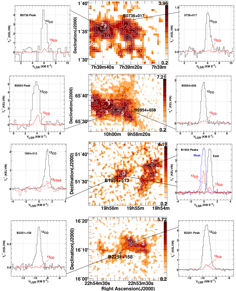
Figure 1: $\mathrm{{}^{12}CO}$ and $\mathrm{{}^{13}CO}$ emission around B0736, B0954, B1954 and B2251. In the center are maps of ${\rm W}_{\rm CO}$ with the positions of the continuum source and one or more emission peaks indicated. Spectra toward the continuum and the peak positions are shown to either side. The contours are at levels 1,2 .. 7 $\mathrm{\,K\,km\,s^{-1}}$ and the color scale on the maps at center varies between 0.2 $\mathrm{\,K\,km\,s^{-1}}$ and the peak value as shown at the upper end.

2 Observations and modelling

2.1 New data

The new data shown here were taken at the ARO Kitt Peak 12m telescope during several observing runs in December or April during the period 2010-2012. Table 1 reprises some general target and sightline characteristics; coordinates, reddening, etc. Table 2 shows positions and profile integrals for the individiual sightlines that furnish the observational material.

The ARO data are presented in terms of the customary brightness scale ${\rm T}_{\rm r}^{*}$ extrapolated outside the atmosphere and nominally corrected for primary beam efficiency by an increase of a factor 1/0.85. As noted by Liszt et al. (2009) this scale is commensurate with the main beam brightness temperature scale of the Nanten telescope, as empirically verified by comparing observations with both instruments over the L121 cloud near $\zeta$ Oph. The LSR velocity scale uses the common kinematic definition that is universally employed at radio telescopes.

The new observations mostly consist of pointed, position-switched observations of species other than $\mathrm{{}^{12}CO}$ toward peaks found in maps of $\mathrm{{}^{12}CO}$ emission around the positions of compact extragalactic continuum sources used to study mm-wave absorption. The $\mathrm{{}^{12}CO}$ maps used as finding charts were discussed in Liszt & Pety (2012) and the new observations should be understood in context with reference to their Figures showing the placement of the background targets maps of galactic reddening, noting their separation from regions of high extinction. However, we also observed at positions of $\mathrm{{}^{12}CO}$ peaks toward portions of the L121 cloud that we identified in new ARO Kitt Peak 12m maps of $\mathrm{{}^{12}CO}$ emission, and we made an on-the-fly map of $\mathrm{{}^{13}CO}$ emission in the field around B0528-134. Nearby off-source positions for position-switching were already known from the extensive mapping we had done.

Observations toward all sources are discussed individually in the ensuing text but the overall goal of understanding the sytematics of CO emission from diffuse molecular gas is really only approachable when the full ensemble of observations is examined.

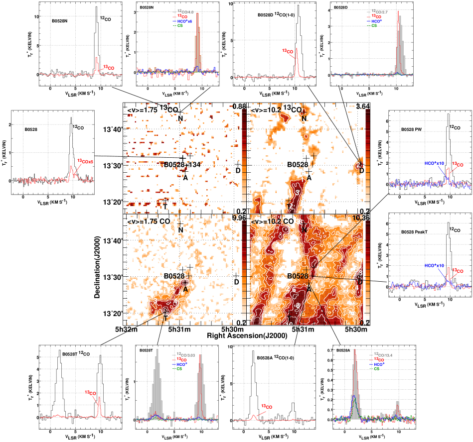
Figure 2: Molecular emission around B0528+134. At center are maps of $\mathrm{{}^{13}CO}$ in the upper row and $\mathrm{{}^{12}CO}$ at bottom, with the blue shifted gas at left and the red-shifted emission at right. The continuum and other selected locations are marked, with lines directed to the spectra at those positions. In some cases the same position is represented by two plots of spectra. Contours are at levels 1,2, 3, 4, 6, 8 and 10 $\mathrm{\,K\,km\,s^{-1}}$.

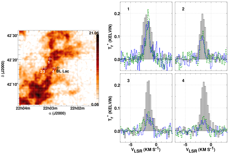
Figure 3: Molecular emission around BL Lac. At left is a map of ${\rm W}_{\rm CO}$, on which are marked the locations of BL Lac and four positions whose CO, $\mathrm{HCO^{+}}$, and CS spectra are shown at right. The CO profiles at right, shown gray and shaded, have been scaled downward by a factor 30. $\mathrm{HCO^{+}}$ is shown as a blue histogram with full lines, CS is shown dashed and green.

Most of the new CO observations are of $\mathrm{{}^{13}CO}$, as the CO hotspots had previously only been observed in $\mathrm{{}^{12}CO}$. But we also searched for $\mathrm{C^{18}O}$ emission in some directions and we made extensive observations of the J=1-0 line of $\mathrm{HCO^{+}}$ and more limited observations of CS J=2-1. The 1-0 lines of HCN, HNC, and C₂H were observed toward Peak 1 near BL Lac and are shown for the sake of completeness in Appendix B where their profile integrals are given. The ${\rm W}_{\rm HCN}$/${\rm W}_{\rm CO}$ ratio at Peak 1 around BL Lac, $0.017\pm 0.001$, is discussed in Section 6.7.

All of the new pointed observations were observed at higher spectral resolution and smoothed to 49 kHz resolution or 0.13 km s^-1 at 115.3 GHz. The $\mathrm{{}^{13}CO}$ OTF mapping around B0528 had a resolution of 100 kHz or 0.27 km s^-1. In the comparisons below, some CO peaks were only observed in $\mathrm{{}^{12}CO}$ during the earlier OTF mapping and these profiles have a resolution 100 kHz (0.26 km s^-1 at 115.3 GHz).

2.2 Existing data

We show emission profiles from the CO mapping around continuum sources from which many of the peaks observed here were first identified (Liszt & Pety, 2012) and we show pointed observations taken with higher spectral resolution toward the continuum sources themselves. We discuss CO line profile integrals toward a wider sample of continuum background sources observed by Liszt & Lucas (1998) (labelled PdBI or PdBI sightlines) and from the CO emission survey toward common UV absorption targets of Liszt (2008) and labelled “Survey 2008”. Some CO emission data closer to $\zeta$ Oph were discussed by Liszt (1997) and these are labelled $\zeta$ Oph$\pm 30$^′. We also discuss the “Mask 1” subset of CO emission brightnesses at low extinction in Taurus observed by Goldsmith et al. (2008).

In Section 6 we derive molecular hydrogen number and colum densities by comparing emission and absorption profiles of the $\mathrm{HCO^{+}}$ J=1-0 line, mostly taken from the work of Lucas & Liszt (1996) but augmented in a few cases with newer NOEMA absorption profiles of higher sensitivity and spectral resolution.

2.3 Modeling

In what follows we compare the observations with recently-published models of CO formation, excitation and fractionation (Liszt, 2017). The models self-consistently calculate the equilibrium abundances of $\mathrm{{\rm H}_{2}}$ (Liszt, 2015) and CO (Liszt, 2007) and their isotopologues in uniformly illuminated, uniform density media having spherical geometry, in the presence of photodissociation, self- and mutual shielding, and exchange of carbon isotopes by the reaction of C⁺ and CO. All aspects of the illumination (optical/UV, cosmic-ray, X-ray) are scaled by a parameter G₀  = 1/3, 1/2 and 1. The CO chemistry is modeled under the simple assumption that the observed quantity of $\mathrm{HCO^{+}}$, N($\mathrm{HCO^{+}}$)/N($\mathrm{{\rm H}_{2}}$) $=3\times 10^{-9}$ (Liszt et al. (2010) and Liszt & Gerin (2016)) recombines to form CO at the local kinetic temperature that is self-consistently computed in the models (Wolfire et al., 1995, 2003). It is actually possible to check the usefulness of this approach given the observed $\mathrm{HCO^{+}}$ emission as described in Section 5.1. This is because the formation of CO from the recombination of $\mathrm{HCO^{+}}$ and the rotational excitation of $\mathrm{HCO^{+}}$ both arise from the interaction of $\mathrm{HCO^{+}}$ with free electrons.

The isotopologic abundance ratios $\mathrm{HCO^{+}}$/H¹³CO⁺/HC¹⁸O⁺ in the model are taken as 1:1/62:1/520 so that the CO isotopolgues are formed in the same proportion as the inherent isotopic abundance ratios in the gas. It is not possible to fractionate $\mathrm{HCO^{+}}$ through its chemical isotopic exchange reactions with CO (Roueff et al., 2015) in diffuse gas where the electron abundance is high, most of the carbon is in C⁺ and the abundance of CO is small: This is the case because, unlike in dark clouds, $\mathrm{HCO^{+}}$ recombines with electrons thousands of times more rapidly than it reacts with CO. The CO isotopologues are fractionated after formation through the processes of selective photodissociation and carbon isotope exchange at the local kinetic temperature.

3 Fields observed

The observed sample of CO hotspots is comprised of two parts; i) observations of gas within 5-30^′ of the positions of compact extragalactic continuum sources used to study molecular absorption at radio wavelengths, and ii) observations over a region of extent 90^′ toward the translucent cloud L121 southwest of the star $\zeta$ Oph. Except for the continuum source B0528-134 that is observed through the Eridanus Loop, the gas seen around the continuum background sources is well removed from regions showing A_V $\gtrsim$ 1 mag. As shown in Figure 1 of Liszt & Pety (2012), B0954+658 (E_B-V = 0.12 mag) and B2251+158 (E_B-V = 0.10 mag) are within a few degrees of MBM 23 and MBM 55 (Magnani et al., 1985) having E_B-V = 0.13 and 0.29 mag, respectively. B1954+513 (E_B-V = 0.15 mag) and B0736+017 (E_B-V = 0.13 mag) are more isolated. The material studied here samples the diffuse, occasionally partially-molecular ISM that is broadly distributed outside dark/molecular cloud complexes.

By contrast, L121 in Ophiuchus is only 1^o-2^o removed from a very extended optically-opaque filament L204 whose CO emission is redshifted by some 4 km s^-1, as shown in Fig. 1 of Liszt et al. (2009). The fact that L121 and L204 had such comparable CO brightnesses was a strong motivating factor for this work.

3.1 Four fields around compact mm-wave continuum sources

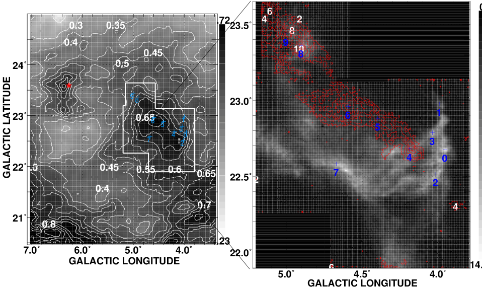
Figure 4: Reddening and CO emission in the vicinity of $\zeta$ Oph, L121 and L204 (Liszt et al., 2009). Left side panel: A map of E_B-V Schlegel et al. (1998) with contours in steps of 0.05 mag and a gray scale running from 0.23 to 0.72 mag as indicated on the adjacent bar scale. The position of the star $\zeta$ Oph is marked by a red asterisk and the portion of L121 mapped in $\mathrm{{}^{12}CO}$ emission at the ARO 12m at 1^′ spatial resolution is outlined. Indicated in blue in both panels are 10 labelled locations Z0..Z9 ordered in galactic longitude where additional pointed observations with higher spectral resolution were taken (see Figure 5 and Table A1). A small part of the filamentary cloud L204 is visible as the high extinction region at lower left. Right side panel: ARO $\mathrm{{}^{12}CO}$ maps of CO emission from L121 at 1^′ resolution on an expanded spatial scale. This panel is a composite of a gray scale representation of integrated emission at v $<$ -0.7 km s^-1 with peak ${\rm W}_{\rm CO}$ = 14.8 $\mathrm{\,K\,km\,s^{-1}}$, and contours in red at levels 2, 4, .. 14 $\mathrm{\,K\,km\,s^{-1}}$ representing the integrated emission at v $>-0.7$ km s^-1.

Figure 1 shows results for CO and $\mathrm{{}^{13}CO}$ around the positions of four extragalactic continuum sources. In the center column are cut-outs of the larger CO maps shown in Liszt & Pety (2012) with peak positions and the location of the continuum marked by crosses. The peak integrated brightness of the $\mathrm{{}^{12}CO}$ emission is shown at the top of the color bar scale at the right side of each map: these vary from 4-7 K-km s^-1. To either side, profiles taken toward the continuum or at the nearby peaks are shown, with connecting lines drawn between the positions of CO peaks and the boxes containing the profiles observed there. As noted in the earlier work, CO lines have typical brightness 1-2 K toward the continuum, and CO peaks of remarkably similar brightness 4-5 K nearby. $\mathrm{{}^{13}CO}$ is detected at most of the positions and is remarkably bright toward the western, blue-shifted CO peak near B1954+513. This was by chance the very first position observed in $\mathrm{{}^{13}CO}$ in the course of this work. However similar the CO brightnesses of the peaks may be around B1954+513, the $\mathrm{{}^{13}CO}$ brightness varies by more than a factor 5.

3.2 The field around B0528+134

A more extensive set of observations around B0528+134 is shown in Figure 2. In the center are four map panels representing $\mathrm{{}^{13}CO}$ emission at top and $\mathrm{{}^{12}CO}$ below, each species sampled over two velocity ranges corresponding to the blue-shifted gas around 1.75 km s^-1 at left and the redshifted component at 9-12 km s^-1 at right. Connecting lines are drawn between map locations and the boxes containing the spectra there, and the same position is sometimes represented by two boxes with different contents and/or scaling of the brightness.

The line of sight to B0528+134 passes near the Eridanus Loop and is not characterized by especially small extinction; E_B-V = 0.89 mag in Table 1. However, the $\mathrm{HCO^{+}}$ column density measured in absorption is smaller than that seen toward BL Lac at E_B-V = 0.32 mag, indicating locally diffuse conditions. The CO emission pattern around B0528+134 is characterized by very regular striations of a component at 9-12 km s^-1 having high contrast and very high CO peak brightnesses typically near 10 K, shown over a wider field by Liszt & Pety (2012). This may be the second example of a phenomenon originally seen in Orion (Berné et al., 2010) and ascribed to “ ‘waves’ at the surface of the Orion molecular cloud, near where massive stars are forming.” Alternatively, striations in molecular gas are discussed by (Heyer et al., 2016) and (Tritsis et al., 2018) and ascribed to some combination of instability, MHD waves and alignment with the magnetic field.

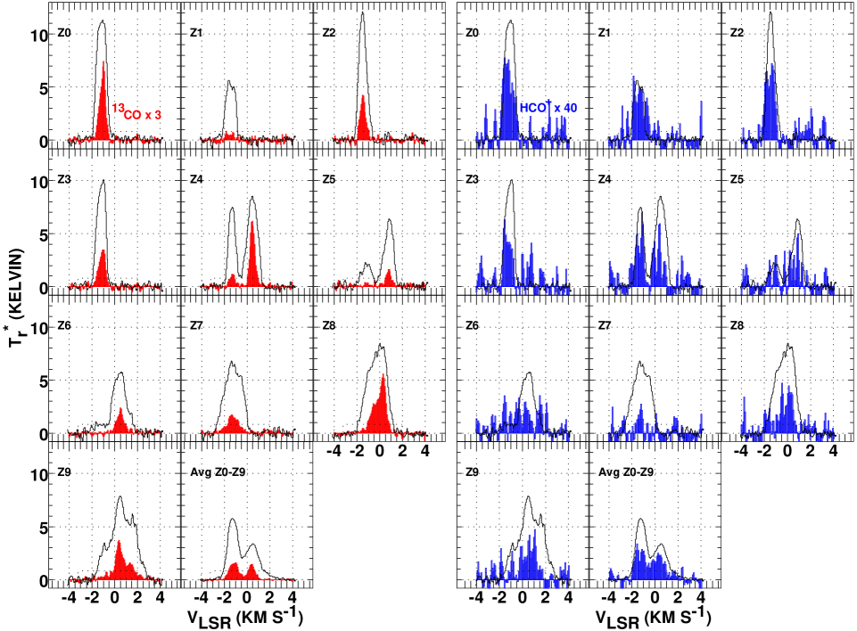
Figure 5: $\mathrm{{}^{12}CO}$, $\mathrm{{}^{13}CO}$, and $\mathrm{HCO^{+}}$ emission from 10 pointings in L121 and their unweighted average at bottom right in each panel. At left $\mathrm{{}^{13}CO}$ emission scaled upward by a factor 3 is shown in red overlaid on CO, while at right $\mathrm{HCO^{+}}$ shown in blue and scaled upward by a factor 40 is overlaid on CO.

As shown in the CO maps in the lower row at the center in Figure 2, the blue-shifted component overlaps a limited portion of the red-shifted emission to the southeast of the continnum and is absent elsewhere. This similarity of morphology suggests a physical connection but the conditions in the red and blue-shifted gas are dissimilar. Comparing the upper and lower maps in either column, one sees that the blue-sshifted gas in the left-hand column is much fainter in $\mathrm{{}^{13}CO}$. Observations at the position B0528T shown in boxes at the lower left corner of Figure 2 illustrate the complexity of the variation in the line brightneses. At a position where both the red and blue components are equally bright in $\mathrm{{}^{12}CO}$ the red peak is much brighter in $\mathrm{{}^{13}CO}$. To the blue where $\mathrm{{}^{13}CO}$ is weaker, $\mathrm{{}^{13}CO}$, $\mathrm{HCO^{+}}$ and CS are all about equally bright. To the red, $\mathrm{{}^{13}CO}$ is an order of magnitude brighter than $\mathrm{HCO^{+}}$ and CS is not detected. Variations in the $\mathrm{HCO^{+}}$/CS brightness ratio are indicative of large differences in their relative abundances as discussed by Liszt (2012) and in more detail in Section 5.2.

3.3 The field around BL Lac

Figure 3 shows profiles at four positions near BL Lac, as marked on a cutout of the $\mathrm{{}^{12}CO}$ map shown in Liszt & Pety (2012). Profiles of $\mathrm{{}^{12}CO}$ scaled downward by a factor of 30 are shown as grey histograms with profiles of $\mathrm{HCO^{+}}$ J=1-0 in red and CS J=2-1 in blue and dashed. Unlike most of the other directions observed here, ie the positions sampled around B0528-134 in Figure 2 (see Section 5.2), $\mathrm{HCO^{+}}$ and CS emission have comparable brightness at all four locations. $\mathrm{{}^{13}CO}$ observations at these positions were thwarted when a snowstorm bore down on the mountain on the day of the Newtown School shootings in December 2012 during the final observing run of this program. The peak integrated brightness of the $\mathrm{{}^{12}CO}$ emission is 21 K-km s^-1, which seems remarkable given that the peak redddening is E_B-V = 0.36 mag in this region (Liszt & Pety, 2012).

3.4 L121

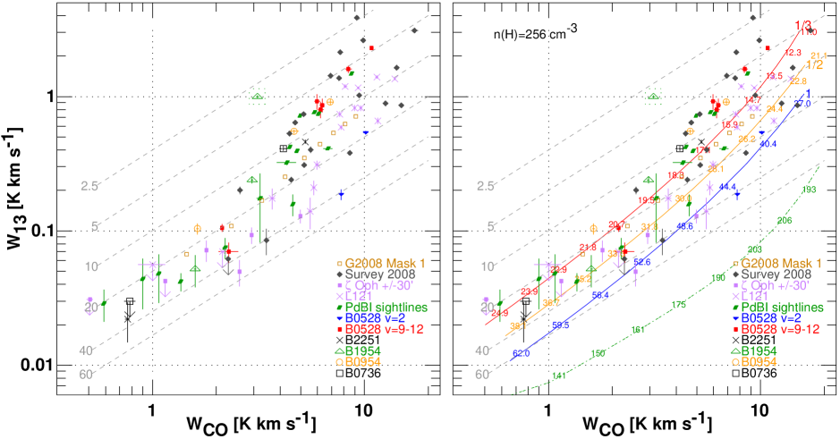
Figure 6: $\mathrm{{}^{13}CO}$ and $\mathrm{{}^{12}CO}$ emission for various datasets. Fiducial values of the ${\rm W}_{\rm CO}$/${\rm W}_{\rm 13}$ ratio are shown as grey dashed lines. Right: with model results superposed for n(H) = 256 $~{}{\rm cm}^{-3}$ and three scaled strengths of the illuminating radiation field, at full, one-half and one-third strength (G₀  = 1, 1/2, and 1/3 respectively). Results neglecting isotope exchange for G₀ =1 are shown as a green dash-dotted line. The numbers along the model curves are the N(CO)/N($\mathrm{{}^{13}CO}$) column density in the model, for comparison with the intensity ratio that is plotted. In general the brightness and column density ratios track each other even when they are much smaller than the inherent isotopic abundance ratio of C/¹³C = 62.

Figure 4 gives an overview of the observing done in the L121 region near $\zeta$ Oph (Liszt et al., 2009). At left is a map of reddening E_B-V using the data of Schlegel et al. (1998) with the star marked by a red asterisk to the northeast. The minimum reddening 0.23 mag must largely be associated with foreground and background material: The material associated with L121 contributes about 0.65-0.23 = 0.4 mag of reddening, or some 1.2 magnitudes of visual extinction in a region where the peak reddening E_B-V = 0.65 mag indicates 2 magnitudes of visual extinction.

CO was mapped over the region outlined at left in Figure 4 by stitching together numerous OTF tiles of size approximately 30^′ x 30^′. The grey scale at right with a peak of ${\rm W}_{\rm CO}$ = 15 K-km s^-1 represents the integrated CO profile of the blue-shifted CO emission at v $\leq-0.7$ km s^-1: the contours in red are for the red-shifted emission at v $>-0.7$ km s^-1 that is rather distinct from the more blue-shifted emission. Both components are observed in optical absorption and radiofrequency emission toward the star $\zeta$ Oph itself. Numbers in white in the right-side frame in Figure 4 are the integrated brightness of the red-shifted emission which peaks just above 10 K-km s^-1 to the north.

Indicated at left and right in Figure 4 are ten locations labeled 0..9 in order of increasing galactic longitude at which pointed observations of CO, $\mathrm{{}^{13}CO}$ and $\mathrm{HCO^{+}}$ were taken, as shown in part in Figure 5. Positions 0 and 9 were observed in $\mathrm{C^{18}O}$ and a few positions were also observed in CS. CO, $\mathrm{{}^{13}CO}$ and $\mathrm{HCO^{+}}$ profiles toward the 10 enumerated positions and their unweighted mean are shown in Figure 5. At left, $\mathrm{{}^{13}CO}$ profiles scaled upward by a factor three are overlaid on $\mathrm{{}^{12}CO}$. At right, $\mathrm{HCO^{+}}$ profiles scaled upward by a factor 40 are overlaid on $\mathrm{{}^{12}CO}$. As with the other fields, CO components with similar ${\rm W}_{\rm CO}$ have widely varying $\mathrm{{}^{13}CO}$ brightness.

4 Results for CO isotopologues

4.1 C¹³O and ¹²CO

Figure 6 shows a summary of the new and existing observations of CO and $\mathrm{{}^{13}CO}$ in diffuse molecular gas: the new data discussed here have been added to the comparable Figure 4 in Liszt (2017). The brightest $\mathrm{{}^{12}CO}$ lines in diffuse/translucent gas generally have ${\rm W}_{\rm CO}$ $\approx$ 10 K-km s^-1 corresponding to N(CO) $\approx 10^{16}~{}{\rm cm}^{-2}$. Exceptions occur in the larger field around BL Lac (Figure 3), toward L121 when the CO line is broad and the red and blue shifted components cannot be separated (Table 2 and Figure 5), and for a few sightlines toward stars used as UV absorption line targets. Many of the smallest ratios ${\rm W}_{\rm CO}$/${\rm W}_{\rm 13}$ $<5$ and the largest ${\rm W}_{\rm CO}$ values arise along sightlines toward UV absorption line targets, in which case CO emission likely originates from dense placental material situated behind the stellar targets: stars seen behind gas emitting very bright CO lines would likely have been too heavily extincted to serve as good UV absorption line targets.

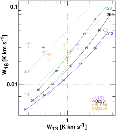
Figure 7: Observed and calculated $\mathrm{C^{18}O}$ and $\mathrm{{}^{13}CO}$ emission profile integrals. Fiducial values of the ratio ${\rm W}_{\rm 13}$/W₁₈ = 20, 40 and 60 are shown as grey dashed lines. Also shown are calculated brightnesses for n(H) = 128 (green), 256 (black) and 512 (blue) $~{}{\rm cm}^{-3}$ at full strength and as a dotted black line for n(H) = 256 $~{}{\rm cm}^{-3}$ with the radiation field at half-strength, showing that the brightness ratio scales as G₀ /n(H). Numbers along the curves indicate the intrinsic N($\mathrm{{}^{13}CO}$)/N($\mathrm{C^{18}O}$) ratio. The intrinsic ¹³C$/^{18}$O ratio in the gas is 520/62 = 8.4.

With the notable exception of one datapoint with very strong $\mathrm{{}^{13}CO}$ emission near B1954+513 (Figure 1), the diverse observational samples provide a consistent overall picture whereby ${\rm W}_{\rm 13}$/${\rm W}_{\rm CO}$ $\approx 1/40-1/20$ at ${\rm W}_{\rm CO}$ $\lesssim 4$ K-km s^-1, increasing so that ${\rm W}_{\rm 13}$/${\rm W}_{\rm CO}$ $\approx 1/20-1/5$ at ${\rm W}_{\rm CO}$$\gtrsim 4$ K-km s^-1.

To understand the observations we show at right in Figure 6 the same data with model results for gas of total density n(H) = 256 $~{}{\rm cm}^{-3}$ and three values of the scaled strength of the incident radiation field G₀ =1, 1/2 and 1/3: the underlying assumptions and methods of the models are discussed in Section 2.3. Along each model curve there are numbers representing the ratio of column densities N($\mathrm{{}^{12}CO}$)/N($\mathrm{{}^{13}CO}$) in the model. These can be compared with the intensity ratios in the plot to assess the degree to which the CO column densities and emission brightnesses track each other, as stressed in Liszt (2017). To aid in this comparison, fiducial lines are shown at fixed intensity ratios 20, 40 and 60.

In the righthand panel in Figure 6 the lowest-lying model curve shows results when the carbon isotope exchange is ignored: Clearly, the success of the models depends most nearly on this process, and very nearly all of the observed $\mathrm{{}^{13}CO}$ is formed from the reaction of ¹³C⁺ with $\mathrm{{}^{12}CO}$, not from the recombination of H¹³CO⁺ with electrons. A comparable situation arises for HD that is almost entirely formed in situ in the gas through gas-phase exchange reactions of deuterium and hydrogen (Liszt, 2015) although, in that case, HD is largely self-shielding (Le Petit et al., 2002).

The effects of changing the density and radiation field are complex in models where the heating is largely through the photoelectric effect on small grains, from photons of about the same energy as those that ionize carbon and photodissociate $\mathrm{{\rm H}_{2}}$ and CO. Slower photodissociation and lower kinetic temperature each encourage more effective carbon isotope exchange while lower temperatures cause faster recombination of $\mathrm{HCO^{+}}$ to CO, weakening the fractionation while allowing a given N(CO) to form at lower n(H), N(H) and N($\mathrm{{\rm H}_{2}}$). At a given ${\rm W}_{\rm CO}$ the ${\rm W}_{\rm 13}$/${\rm W}_{\rm CO}$ integrated brightness ratio increases with higher density and weaker illumination, with a progressively stronger density dependence at amaller values of G₀ . The highest observed values of ${\rm W}_{\rm 13}$/${\rm W}_{\rm CO}$ require some combination of higher density and weaker radiation and the effect of dimming the radiation is stronger at the higher densities.

For ${\rm W}_{\rm CO}$ $\lesssim$ 4 K-km s^-1 where ${\rm W}_{\rm 13}$/${\rm W}_{\rm CO}$ $\approx 1/40-1/20$ the data can generally be explained at any number density n(H) $\gtrsim 128~{}{\rm cm}^{-3}$, but even the lowest of these densities is already large enough that the molecular fraction $<{\rm f}_{\mathrm{{\rm H}_{2}}}>$ = 2N($\mathrm{{\rm H}_{2}}$)/N(H) $\gtrsim$ 0.7 according to Figure 6 of Liszt (2017).

The isotopologic intensity ratio ${\rm W}_{\rm CO}$/${\rm W}_{\rm 13}$ tracks the column density ratio N(CO)/N($\mathrm{{}^{13}CO}$) even when both ratios are much less than 62 and the proportionality between brightness and column density persists well beyond the domain where $\tau>1$ as long as the excitation is strongly sub-thermal (Goldreich & Kwan, 1974). The difference between ${\rm W}_{\rm CO}$/${\rm W}_{\rm 13}$ and N(CO)/N($\mathrm{{}^{13}CO}$) is about 20% at ${\rm W}_{\rm CO}$ = 5 K-km s^-1 or 40% at ${\rm W}_{\rm CO}$ = 10 K-km s^-1, with slightly larger differences at smaller G₀ . The point is that when the isotopologic brightness ratio significantly departs from 62, the actual abundance ratio is much closer to the observed brightness ratio than to the intrinsic isotopic abundance ratio. N($\mathrm{{}^{12}CO}$) cannot be reliably estimated from comparing the $\mathrm{{}^{12}CO}$ and $\mathrm{{}^{13}CO}$ brightnesses under the common assumption that both isotopologues are present in the intrinsic ratio, and the wide variations in N(CO)/N($\mathrm{{\rm H}_{2}}$) in any case mean that N(CO) cannot be used to infer N($\mathrm{{\rm H}_{2}}$) in any case. This point was stressed by Szucs et al. (2016) who concluded that it was more accurate to derive N($\mathrm{{\rm H}_{2}}$) by scaling ${\rm W}_{\rm CO}$ with a CO-$\mathrm{{\rm H}_{2}}$ conversion factor. If desired, the carbon monoxide column densities can be estimated as N(CO) $=10^{15}~{}{\rm cm}^{-2}$ ${\rm W}_{\rm CO}$ and similarly for other isotopologues.

Two aspects of the data in Figure 6 deserve comment insofar as they relate to a comparison with UV absorption line data as discussed by (Liszt, 2017). The nearly constant ratio N(CO)/N($\mathrm{{}^{13}CO}$) $\approx 65$ seen in UV absorption at N(CO) $<10^{16}~{}{\rm cm}^{-2}$ is higher than that inferred from mm-wave emission brightness ratios and corresponds most closely to the curves for G₀ =1: The gas observed in optical absorption is mostly unfractionated, from which we infer that it is subject to a stronger radiation field and is warmer and less dense than that observed in mm-wave emission. Conversely, the CO emission data taken in directions toward the same early-type stars that are observed in UV absorption (Liszt, 2008) require a diminished radiation field at the density n(H) = 256 $~{}{\rm cm}^{-3}$ that was used in Figure 6. The counter-intuitive inference of a weaker radiation field is consistent with the notion that strong CO emission toward the absorption line stars arises in dense fully-molecular gas behind the star because these stars would not have been suitable UV absorption targets with the opposite geometry. $\zeta$ Oph is a case where little or none of the molecular emission observed in its direction arises behind the star, but the emission is weak, ${\rm W}_{\rm CO}$ $\approx$ 1 K-km s^-1.

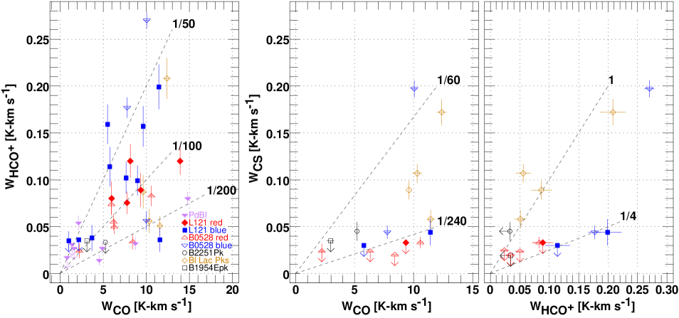
Figure 8: Observed $\mathrm{{}^{12}CO}$, $\mathrm{HCO^{+}}$, and CS profile integrals. Fiducial values are shown as grey dashed lines.

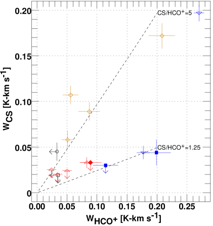
Figure 9: As in the right-most panel of Figure 8, but with model results for two values of the abundance ratio, CS/$\mathrm{HCO^{+}}$ = 5 and 5/4. Calculated results are not perceptibly different for different density n(H) and illumination G₀ .

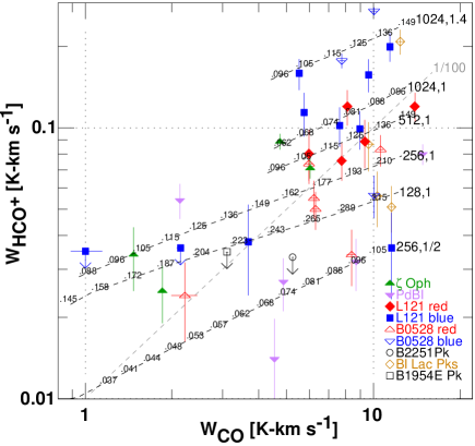
Figure 10: Observed $\mathrm{{}^{12}CO}$ and $\mathrm{HCO^{+}}$ line profile integrals on a logarithmic scale with model results. Labels at the right hand side of each model curve represent n(H) in units of $~{}{\rm cm}^{-3}$ and the radiation field scaling parameter G₀ . Numbers along the model curves are the reddening E_B-V. A fiducial line with W${}_{\mathrm{HCO^{+}}}$/${\rm W}_{\rm CO}$ = 0.01 is shown grayed and dashed.

4.2 C¹⁸O

Few measurements of absorption by $\mathrm{C^{18}O}$ are available in the UV, but two sightlines with N(CO) $=2\times 10^{15}~{}{\rm cm}^{-2}$ and $=2.5\times 10^{16}~{}{\rm cm}^{-2}$ show $\mathrm{C^{18}O}$ depletions of 3 and 6, respectively, with respect to the ratio N(CO)/N($\mathrm{C^{18}O}$) = 520 (see Figure 1 of (Liszt, 2017)). The mm-wave measurements presumably sample gas with weaker radiation fields and weaker selective photodissocation of $\mathrm{C^{18}O}$.

Figure 7 shows the limited amount of meaningful data we have been able to gather on the integrated intensity of $\mathrm{C^{18}O}$, W₁₈, compared with ${\rm W}_{\rm 13}$. Also shown in Figure 7 are calculated brightnesses for n(H) = 128, 256 and 512 $~{}{\rm cm}^{-3}$ with the radiation field at full strength and at n(H) = 256 $~{}{\rm cm}^{-3}$ with G₀  = 1/2, Given along the curves showing model results are the intrinisic N($\mathrm{{}^{13}CO}$)/N($\mathrm{C^{18}O}$) ratios: these can be compared with the model brightness ratios to see that the observed brightness ratios can straightforwardly be interpreted as column density ratios. The model brightnesses are weakly dependent on G₀  and n(H) in opposite senses, falling with G₀ , and the model brightness ratio scales approximately as G₀ /n(H) (the curves coincide for n(H)=512 $~{}{\rm cm}^{-3}$, G₀ =1 and n(H)=256 $~{}{\rm cm}^{-3}$, G₀ =1/2).

$\mathrm{C^{18}O}$ emission is very weak in diffuse molecular gas, with $3\sigma$ observational upper limits ${\rm W}_{\rm 13}$/W${}_{18}>25-40$ in several cases as against an intrinsic isotopic abundance ratio ¹³C/¹⁸O = 520/62 = 8.4. If N($\mathrm{{}^{13}CO}$) is enhanced by a factor g, the implied $\mathrm{C^{18}O}$ depletion factors are (25-40)/8.4/g = (3-5)/g. The limited range of relatively large ${\rm W}_{\rm 13}$ values sampled in Figure 7 corresponds to high values g $\gtrsim 2-4$ (see Figure 6) so the mm-wave measurements disappointingly do not constrain the $\mathrm{C^{18}O}$ depletion at the levels observed in UV absorption spectra.

5 Emission from strongly-polar species HCO⁺ and CS

Figure 8 summarizes the $\mathrm{HCO^{+}}$ and CS J=2-1 observations with respect to each other and with respect to CO. The panel plotting W${}_{\mathrm{HCO^{+}}}$ vs. ${\rm W}_{\rm CO}$ at left shows that $\mathrm{HCO^{+}}$ brightens considerably for ${\rm W}_{\rm CO}$ = 6 - 10 K-km s^-1 but W${}_{\mathrm{HCO^{+}}}$/${\rm W}_{\rm CO}$ = 1/200 - 1/50 quite generally. Such ratios are characteristic of gas in the disk of the inner Milky Way, outside the galactic center (Liszt, 1995; Helfer & Blitz, 1997), and other galaxies (Jiménez-Donaire et al., 2019) as discussed in Section 6.8.

CS J=2-1 emission brightens abruptly at ${\rm W}_{\rm CO}$ $\gtrsim 10$ K-km s^-1 in the middle panel of Figure 8, from data in the blue component around B0528 (see Figure 2) and around BL Lac (Figure 3). The rightmost panel in Figure 8 shows that the W_CS/W${}_{\mathrm{HCO^{+}}}$ ratio is bimodal. The same datapoints toward BL Lac and in the blue component around B0528 having stronger CS emission at ${\rm W}_{\rm CO}$ = 10-12 K-km s^-1 in the middle panel have three-four times larger W_CS/W${}_{\mathrm{HCO^{+}}}$ ratios than the rest of the data, over a wide range of W${}_{\mathrm{HCO^{+}}}$.

The $\mathrm{HCO^{+}}$ J=1-0 and CS J=2-1 line brightnesses are small enough that both are in the weak excitation limit of Liszt & Pety (2016) and the line profile integral may be expressed as a line of sight integral through the emitting medium

$$\int\mbox{$T_{B}$}d{\rm v}=(\lambda^{2}/8\times 10^{5}\pi)(hc/k)\int n(H)\gamma_{u}n(Y)dL$$

where Y stands for $\mathrm{HCO^{+}}$ or CS and $\gamma_{u}$ is an excitation rate per H-nucleus determined by the local temperature and ionization fraction. The emergent line brightness is roughly proportional to the product of the mean number density of hydrogen and the column density of the emitting molecule, not its critical density. Details of the cloud structure and molecular abundance distribution are washed out by the line of sight integration and the emergent line brightnesses are not explictly dependent on the optical depth.

5.1 ${\rm W}_{\rm CS}$/W${}_{\mathrm{HCO^{+}}}$ and N(CS)/N(HCO⁺) are bimodal

The bimodality of the ${\rm W}_{\rm CS}$/W${}_{\mathrm{HCO^{+}}}$ brightness ratio in the right-most panel of Figure 8, with values approximately 1 and 1/4, reflects a real bimodality of the N(CS)/N($\mathrm{HCO^{+}}$) abundance ratio: there is no effect associated with the excitation that can cause such a difference given that both species must coexist in the regions that have higher $\mathrm{{\rm H}_{2}}$ fractions. Shown in Figure 9 are results for the model brightnesses of CS J=2-1 and $\mathrm{HCO^{+}}$ under the assumption that n(CS)/n($\mathrm{HCO^{+}}$) = 5 and n(CS)/n($\mathrm{HCO^{+}}$) = 5/4 everywhere in the models (recall that n($\mathrm{HCO^{+}}$)/n($\mathrm{{\rm H}_{2}}$) $=3\times 10^{-9}$ is fixed while n(H) and n($\mathrm{{\rm H}_{2}}$) vary) and the model results for the intensity ratio are insensitive to n(H).

As discussed in Appendix C, bimodality of the N(CS)/N($\mathrm{HCO^{+}}$) ratio was not observed in our survey of mm-wave $\mathrm{HCO^{+}}$ and CS absorption (Lucas & Liszt, 2002), because the sightlines directly toward continuum sources sample material with CO emission well below the ${\rm W}_{\rm CO}$ values where bimodality is evident in Figure 8. The previously-observed column density ratios N(CS)/N($\mathrm{HCO^{+}}$) derived in absorption have mean $<$N(CS)$>$/$<$N($\mathrm{HCO^{+}}$)$>$ = 1.27 and $<$N(CS)/N($\mathrm{HCO^{+}}$)$>$ = 1.66$\pm$1.32 and are in overall agreement with the column density ratios derived now in emission alone.

Bistability is a recognized phenomenon in chemical networks for dense gas (Le Bourlot et al., 1993; Lee et al., 1998; Charnley & Markwick, 2003; Boger & Sternberg, 2006; Wakelam et al., 2006; Dufour & Charnley, 2019) and the abundance of CS is one of the earliest recognized markers (Le Bourlot et al., 1993). Gerin et al. (1997) found a column density of CS in a core in Polaris at E_B-V $\approx 0.6$ mag that was 20-40 times higher than in Taurus at E_B-V $\gtrsim 1$ mag: the N(CS)/N($\mathrm{HCO^{+}}$) ratio was about a factor two higher in Polaris even as the brightness ratio ${\rm W}_{\rm CS}$/W${}_{\mathrm{HCO^{+}}}$ was smaller by a factor three, being 2 in Taurus and 0.7 in Polaris. The kind of bistability that is discussed for dense gas chemical networks with a contrast between high and low ionization phases driving changes in the abundance of H₃⁺ is not obviously relevant in diffuse molecular gas where CO is a minority constituent, the ionization fraction is high and electron recombination of H₃⁺ is rapid.

5.2 HCO⁺ and CO

On its own terms the $\mathrm{HCO^{+}}$ line brightness is subject to the same considerations of the weak excitation limit as CS, but the special role of $\mathrm{HCO^{+}}$ as the progenitor of CO and its fixed abundance with respect to $\mathrm{{\rm H}_{2}}$ mean that the comparison of ${\rm W}_{\rm CO}$ and W${}_{\mathrm{HCO^{+}}}$ has broader implications for the CO formation chemistry.

As a first approach to interpret the $\mathrm{HCO^{+}}$ data with respect to CO, recall that the rotational excitation of $\mathrm{HCO^{+}}$ is dominated by collisions with electrons in diffuse molecular gas (Liszt, 2012; Liszt & Pety, 2016) where n(e)/n(H) $\approx 2-3\times 10^{-4}$ as the result of photoionization of carbon and a somewhat smaller contribution from cosmic-ray ionization of atomic hydrogen (Draine, 2011). The electron abundance declines at higher density as the H⁺ fraction decreases but n(e) remains high until C⁺ recombines to CO (Liszt, 2011). In this case W${}_{\mathrm{HCO^{+}}}$ $\propto\int n(H)n(\mathrm{HCO^{+}})dL\propto\int n(e)n(\mathrm{HCO^{+}})dL$. However, CO is formed from the thermal recombination of $\mathrm{HCO^{+}}$ with electrons so W${}_{\mathrm{HCO^{+}}}$ is also proportional to the column-averaged CO formation rate. With ${\rm W}_{\rm CO}$ $\propto$ N(CO), the W${}_{\mathrm{HCO^{+}}}$/${\rm W}_{\rm CO}$ brightness ratio is equivalent to taking the ratio of the column-averaged CO formation rate to the resulting CO column density. When this is larger, a higher formation rate is being required to produce a given amount of CO, so the destruction rate must be larger. Viewed in this way, the variation in W${}_{\mathrm{HCO^{+}}}$ at ${\rm W}_{\rm CO}$ = 6-12 K-km s^-1 in the leftmost panel of Figure 8 suggests a wide range in CO photodestruction rates.

Viewed another way, W${}_{\mathrm{HCO^{+}}}$/${\rm W}_{\rm CO}$ $\propto$ $<$n(H)$>$N($\mathrm{HCO^{+}}$)/${\rm W}_{\rm CO}$ $\propto$ $<$n(H)$>$N($\mathrm{{\rm H}_{2}}$)/N(CO), so the W${}_{\mathrm{HCO^{+}}}$/${\rm W}_{\rm CO}$ brightness ratio also samples the relative CO abundance, testing whether the observed CO emission is being produced at reasonable n(H) and N($\mathrm{{\rm H}_{2}}$). The low-light models that fractionate CO more readily in the right-hand panel of Figure 6 will produce a given N(CO) and ${\rm W}_{\rm CO}$ at smaller N($\mathrm{{\rm H}_{2}}$), and so with weaker $\mathrm{HCO^{+}}$ emission.

These two viewpoints are illustrated with calculations of the W${}_{\mathrm{HCO^{+}}}$/${\rm W}_{\rm CO}$ brightness ratio in Figure 10, again showing the data from the left-most panel of Figure 8, but on logarithmic scales. The models with G₀  = 1 run through the base level of $\mathrm{HCO^{+}}$ emission with a relatively weak density dependence that confirms the consistency of the overall CO formation scheme based on recombination of the observed relative abundance of $\mathrm{HCO^{+}}$. The models reproduce the observed $\mathrm{HCO^{+}}$ brightness and CO column density at typical values of the molecular hydrogen column density. The data toward L121 in the field of $\zeta$ Oph are reproduced with a stronger radiation field and a higher density, along with two of the three datapoints in the blue component of B0528 and one point in the field around BL Lac.

With the weaker illumination needed to enhance $\mathrm{{}^{13}CO}$ there is little density dependence in the model W${}_{\mathrm{HCO^{+}}}$/${\rm W}_{\rm CO}$ ratios and one curve is plotted for n(H) $=256~{}{\rm cm}^{-3}$ covering the density range n(H) = 128 - 512 $~{}{\rm cm}^{-3}$ at G₀ =1/2: the reddening values given along the relevant curve scale inversely with n(H). As indicated in Figure 10, and as expected, the low-light models produce a given N(CO) or ${\rm W}_{\rm CO}$ at much smaller N(H) and E_B-V, and with W${}_{\mathrm{HCO^{+}}}$ weaker by about a factor two compared to the models with fuller illumination. The low-light conditions that reproduce N(CO), ${\rm W}_{\rm CO}$ and N($\mathrm{{}^{13}CO}$) at ${\rm W}_{\rm CO}$ $\lesssim 5$ K-km s^-1 account for only about one half of the base level of $\mathrm{HCO^{+}}$ emission W${}_{\mathrm{HCO^{+}}}$ $\approx 0.02-0.03$ K-km s^-1 at ${\rm W}_{\rm CO}$ $\lesssim 5$ K-km s^-1 but with correspondingly smaller total column column density and E_B-V.

The CO hotspots near the mm-wave continuum background sources are explained as embedded, localized regions perhaps with higher density, but even more likely with increased shielding, occupying a small fraction of the volume of the overall diffuse molecular medium. In turn, much or most of the $\mathrm{HCO^{+}}$ emission arises in other material that makes a small contribution to the CO abundance and emission.

5.3 CO hotspots near mm-wave background sources

Enhanced and faster formation of $\mathrm{{\rm H}_{2}}$ and CO in localized regions of greater density and optical shielding are common features of turbulent models of the HI$\rightarrow$$\mathrm{{\rm H}_{2}}$ transition in diffuse molecular gas (Shetty et al., 2011; Godard et al., 2014; Valdivia et al., 2017; Bialy et al., 2019). Most likely the CO hotspots observed near the background mm-wave continuum sources and shown in Figure 1 are examples of this phenomenon. The similarity of the sizes (10^′) and peak brightnesses (5 K-km s^-1) of the hotspots seen in the vicinity of the mm-wave background sources in Figure 1 suggest that common physical phenomena and physical conditions are being sampled. The extraordinarily small ${\rm W}_{\rm CO}$/${\rm W}_{\rm 13}$ ratio (3:1) observed toward the West peak around B1954+513 is in marked contrast to the much larger values, typically 20:1, seen in the other directions. This requires further investigation.

As a specific example, consider that the low-light models with n(H) $=256~{}{\rm cm}^{-2}$ shown in Figure 10 are at most about 80% molecular, ie n($\mathrm{{\rm H}_{2}}$) $\lesssim 100~{}{\rm cm}^{-2}$, and produce 1 K-km s^-1 $\leq$ ${\rm W}_{\rm CO}$$\leq$ 5 K-km s^-1 at 0.04 $\lesssim$ E_B-V$\lesssim$ 0.07 mag. With N(H)/E_B-V $\approx 8\times 10^{21}~{}{\rm cm}^{-2}$(mag)^-1 (Liszt, 2014a, b; Hensley & Draine, 2017) and [C]/[H] $=1.6\times 10^{-4}$ (Sofia et al., 2004), one would expect N(C⁺) $=5.3-9.3\times 10^{16}~{}{\rm cm}^{-2}$. Because the required CO column densities are $1-5\times 10^{15}~{}{\rm cm}^{-2}$ there is ample margin for N(CO) to increase, and CO emission to brighten to levels ${\rm W}_{\rm CO}$ = 5 K-km s^-1, without upsetting the balance of the carbon ionization equilibrium that maintains the preponderance of carbon in C⁺. At a nominal distance of 250 pc as for the field around B2251+158 (Zucker et al., 2019), a region with E_B-V = 0.05 mag and n(H)$=256~{}~{}{\rm cm}^{-2}$ has a size N(H)/n(H) $=4\times 10^{20}~{}{\rm cm}^{-2}/256~{}{\rm cm}^{-3}=0.51$ pc, subtending an angular size 8.0^′. This is a typical size for the regions of enhanced CO emission in Figure 1.

The required N(H) and E_B-V scale inversely with the density, so the implied angular size would vary approximately as 1/n(H)². The surrounding medium could be an order or magnitude more expansive with a factor $\gtrsim 3$ density contrast that would suffice to lower the molecular fraction and substantially weaken the CO emission (Liszt, 2017). These scalings are important to understanding the presence of the CO hotspots along lightly-reddened sightlines, in the absence of evidence for variations in the reddening comparable to the contrasts in ${\rm W}_{\rm CO}$. It is not necessary to imagine a contraction of the entire medium into clumps as small as the CO emission regions shown in Figure 1.

6 Summary and discussion

6.1 $\mathrm{{}^{12}CO}$ and $\mathrm{{}^{13}CO}$

Once upon a time we mapped $\mathrm{{}^{12}CO}$ emission around the locations of a dozen extragalactic mm-wave background continuum sources that had been used to survey for the presence of molecular gas by observing the J=1-0 line of $\mathrm{HCO^{+}}$ in absorption. We noted the presence of quite strong peak profile-integrated CO J=1-0 emission ${\rm W}_{\rm CO}$ $\gtrsim$ 5 K-km s^-1 in regions of very modest reddening E_B-V = 0.1 - 0.3 mag (our CO “hotspots”) when only much weaker CO emission had been seen a few arcminutes away toward the continuum sources themselves.

In this work we followed up by observing $\mathrm{{}^{13}CO}$, $\mathrm{C^{18}O}$, $\mathrm{HCO^{+}}$ and CS J=2-1 emission at positions of strong CO emission in five of these previously-studied regions and we mapped a more extended portion of the L121 cloud south of the bright star $\zeta$ Oph that has frequently been used to study diffuse molecular gas in optical/UV absorption. We also gathered comparable information from the literature to produce a larger sample of observations of the carbon monoxide isotopolgues from diffuse molecular gas covering a wider range of values of the profile-integrated $\mathrm{{}^{12}CO}$ emission brightness ${\rm W}_{\rm CO}$.

Observations of the individual regions observed here were discussed in Section 3 and illustrated in Figures 1-5. The systematics of the carbon monoxide isotopologues were discussed in Section 4 and summarized in Figure 6. As shown in Figure 6 there is a gradual increase in the ${\rm W}_{\rm 13}$/${\rm W}_{\rm CO}$ isotopologic integrated brightness ratio from ${1/40}\leq$ ${\rm W}_{\rm 13}$/${\rm W}_{\rm CO}$ $\leq{1/20}$ at 0.8 K-km s^-1 $\lesssim$ ${\rm W}_{\rm CO}$ $\lesssim 4$ K-km s^-1 to higher values 1:15 - 1:5 with much larger scatter (factor 5) at larger ${\rm W}_{\rm CO}$. Carbon monoxide column densities and line brightnesses are largely synonymous, with ${\rm W}_{\rm CO}$ $\approx$ N(CO)/$(10^{15}~{}{\rm cm}^{-2})$ for ${\rm W}_{\rm CO}$ $\lesssim 5$ K-km s^-1 and N(CO) $\lesssim 5\times 10^{15}~{}{\rm cm}^{-2}$ at densities n(H) $\gtrsim 100~{}{\rm cm}^{-2}$ for all isotopologues. The implication, made clear in the right side panel in Figure 6 showing both ratios for both the column density and intensity ratios, is that the isotopologic intensity ratios observed at ${\rm W}_{\rm CO}$ $\lesssim 5$ K-km s^-1 are very close to the ratio of column densities even when comparatively large values 1/40 $\lesssim$ ${\rm W}_{\rm 13}$/${\rm W}_{\rm CO}$ $\lesssim$ 1/15 are observed. Departures from the intrinsic ratio ${}^{13}C$/${}^{12}C$ = 1/62 result from isotopic C⁺ exchange that dominates selective photodissociation across the entire observed range in ${\rm W}_{\rm CO}$.

The relationship between CO brightness and column density flattens for ${\rm W}_{\rm CO}$ $\gtrsim$ 5 K-km s^-1 where N(CO)/${\rm W}_{\rm CO}$ $>10^{15}~{}{\rm cm}^{-2}$ (K-km s^-1)^-1, but substantial enhancement of $\mathrm{{}^{13}CO}$ persists over the entire observed range of ${\rm W}_{\rm CO}$, and whenever C⁺ is the dominant form of gas-phase carbon (and not otherwise). Ratios N($\mathrm{{}^{13}CO}$)/N($\mathrm{{}^{12}CO}$) as small as 1/60 are expected only at very very small N(CO) where there is no self-shielding, in regions of very high UV illumination, or when the gas phase carbon has fully recombined from C⁺ to CO. The only sure way to avoid factor f $>1$ enhancement of $\mathrm{{}^{13}CO}$ is to be certain that the fraction of free gas-phase ${}^{12}C$ in $\mathrm{{}^{12}CO}$ exceeds 1/f. Of course it is pointless to derive N(CO) if the ultimate goal is to determine N($\mathrm{{\rm H}_{2}}$) when the relative CO abundance N(CO)/N($\mathrm{{\rm H}_{2}}$) is as small and variable as it is in diffuse molecular gas.

6.2 $\mathrm{C^{18}O}$

$\mathrm{C^{18}O}$ is observed in UV absorption to be depleted by a factor three below the value N($\mathrm{C^{18}O}$):N($\mathrm{{}^{12}CO}$) = 1:520 corresponding to the intrinsic isotopic relative abundance ratio ¹⁸O/¹²C. We obtained limits ${\rm W}_{\rm 18}$/${\rm W}_{\rm 13}$ $<1/40-1/20$ along a handful of sightlines with bright $\mathrm{{}^{13}CO}$ lines, vs an intrisic ratio ¹⁸O/${}^{13}C=1/8.4$, see Figure 7. Selective photodissociation of $\mathrm{C^{18}O}$ is present in our data but the gas is also enhanced in $\mathrm{{}^{13}CO}$ and the emission observations did not contrain the depletion of $\mathrm{C^{18}O}$ at the levels detected in UV absorption despite the very low brightness levels to which we chased the $\mathrm{C^{18}O}$ emission. Nonetheless high isotopologic brightness ratios ${\rm W}_{\rm 13}$/${\rm W}_{\rm 18}$ are expected to be a hallmark of emission from diffuse molecular gas.

6.3 CS J=2-1 vs. CO and $\mathrm{HCO^{+}}$

In Figure 8 we showed that CS J=2-1 emission abruptly brightens from 0.03 - 0.04 K-km s^-1 to 0.2 K-km s^-1 over a narrow range of CO brightness ${\rm W}_{\rm CO}$ = 10-12 K-km s^-1 and is bimodal with respect to the brightness of $\mathrm{HCO^{+}}$ with a separation of a factor 4. As noted in Section 5.2, The J=2-1 line of CS and the J=1-0 line of $\mathrm{HCO^{+}}$ are both in the weak excitation limit where ${\rm W}_{\rm CS}$ and W${}_{\mathrm{HCO^{+}}}$ are proportional to N(CS) and N($\mathrm{HCO^{+}}$), respectively, so the bimodality of the brightnesses represents bimodality of the N(CS)/N($\mathrm{HCO^{+}}$) ratio with values 5 and 1.25, as indicated in Figure 9. Bistable chemical solutions for sulfur-bearing molecules are now well-studied for dense gas but are not expected in diffuse molecular gas where the electron fraction is high.

6.4 $\mathrm{HCO^{+}}$ and CO

Comparisons between ${\rm W}_{\rm CO}$ and W${}_{\mathrm{HCO^{+}}}$ are shown in Figure 8 at left, and, on a logarithmic scale with model results superimposed, in Figure 10. As discussed in Section 5.2, $\mathrm{HCO^{+}}$ plays a special dual role as progenitor of CO via thermal recombination with ambient electrons and as an $\mathrm{{\rm H}_{2}}$-tracer with fixed relative abundance N($\mathrm{HCO^{+}}$)/N($\mathrm{{\rm H}_{2}}$) $=3\times 10^{-9}$. Given that the $\mathrm{HCO^{+}}$ emission line brightness W${}_{\mathrm{HCO^{+}}}$ $\propto$ N($\mathrm{HCO^{+}}$) $\propto$ N($\mathrm{{\rm H}_{2}}$) is mostly due to rotational excitation by electrons with which $\mathrm{HCO^{+}}$ also recombines to form CO, W${}_{\mathrm{HCO^{+}}}$ traces N($\mathrm{{\rm H}_{2}}$) while the W${}_{\mathrm{HCO^{+}}}$/${\rm W}_{\rm CO}$ brightness ratio traces both the CO photodestruction rate and the CO abundance relative to $\mathrm{{\rm H}_{2}}$. The chemical model that explains the presence of CO through $\mathrm{HCO^{+}}$ recombination also accounts for the baseline level of $\mathrm{HCO^{+}}$ emission 0.03 K-km s^-1 and log(W${}_{\mathrm{HCO^{+}}}$/${\rm W}_{\rm CO}$) $=-2\pm 0.3$ at modest density n(H) $\approx 100~{}{\rm cm}^{-3}$. The peak $\mathrm{HCO^{+}}$ brightness and the scatter in the W${}_{\mathrm{HCO^{+}}}$/${\rm W}_{\rm CO}$ brightness ratio both increase considerably for ${\rm W}_{\rm CO}$ $\gtrsim$ 10 K-km s^-1. We modeled this as arising from some combination of stronger illumination (increasing the CO photodissociation rate and the required column densities of $\mathrm{{\rm H}_{2}}$ and $\mathrm{HCO^{+}}$ required to produce a given N(CO) and ${\rm W}_{\rm CO}$), and higher density.

The low-light models that strongly fractionate carbon monoxide and enhance $\mathrm{{}^{13}CO}$ are very efficient at producing $\mathrm{{\rm H}_{2}}$ and CO, and reproduce the observed CO column density and brightness ${\rm W}_{\rm CO}$ $\lesssim$ 5 K-km s^-1 at reddening well below even 0.1 magnitudes in Figure 10. The CO hotspots with ${\rm W}_{\rm CO}$ = 5 K-km s^-1 seen in the vicinity of sightlines toward extragalactic continuum sources probably represent the sort of localized regions with higher density and increased optical shielding that are seen in numerical models of turbulent flow in diffuse molecular gas at the HI$\rightarrow$$\mathrm{{\rm H}_{2}}$ transition. In Section 5.3 we gave a numerical example showing that the column densities required to produce the observed CO emission imply mildly sub-pc sized regions subtending angular sizes of about 10^′ ($256~{}{\rm cm}^{-2}$/n(H))^-2 at a distance of 200 pc, as observed. These hotspots are embedded in a more broadly-distributed, weakly CO-emitting, less fully-molecular medium having density a few times lower, which is most easily detected in $\mathrm{HCO^{+}}$ absorption while making a noticeable contribution to the $\mathrm{HCO^{+}}$ emission as discussed in Section 5.2.

6.5 The bright CO emission contribution of diffuse molecular gas

Although more attention has recently been paid to conditions under which CO is not detectable, CO actually radiates exceptionally brightly on a per-molecule basis in subthermally-excited diffuse molecular gas. The CO column density producing ${\rm W}_{\rm CO}$ $\approx 1-10$ K-km s^-1 in diffuse, partially molecular gas, N(CO) $\approx 10^{15}-10^{16}~{}{\rm cm}^{-2}$ is far smaller than from the colder, denser fully-molecular gas in dark clouds, where C⁺ has fully recombined to CO at kinetic temperatures of 10-12 K. At A_V = 5 mag and N(CO)/N($\mathrm{{\rm H}_{2}}$) $=8\times 10^{-5}$, the same brightness would be produced with N(CO) $\approx 5\times 10^{17}~{}{\rm cm}^{-2}$ in a fully molecular gas.

For CO, as with other molecules at the threshold of detectability, column density is the main determining factor. Any density capable of fostering a CO chemistry putting 0.1% or more of the free gas phase carbon into CO at 1 magnitude extinction will put enough energy into the J=1-0 CO line to render its emission detectable at a level ${\rm W}_{\rm CO}$ $\gtrsim 0.1$ K-km s^-1. Detectability at the 1 K-km s^-1 level requires N(CO) $=10^{15}~{}{\rm cm}^{-2}$ for n(H) $\gtrsim 100~{}{\rm cm}^{-3}$, while the expected free gas-phase carbon column density at 1 magnitude of optical extinction is $4\times 10^{17}~{}{\rm cm}^{-2}$, implying that only 2.5% of the free gas-phase carbon need be in CO. For diffuse molecular gas where N(CO) and ${\rm W}_{\rm CO}$ are proxies for each other around the ${\rm W}_{\rm CO}$ = 1 K-km s^-1 threshold of detectability in wide-field surveys, N($\mathrm{{\rm H}_{2}}$)/${\rm W}_{\rm CO}$ $\propto$ N($\mathrm{{\rm H}_{2}}$)/N(CO), and it is the CO abundance that determines the CO-$\mathrm{{\rm H}_{2}}$ conversion factor and the ability of CO to serve as an $\mathrm{{\rm H}_{2}}$ surrogate.

6.6 Dense gas tracers also trace diffuse gas

Species like $\mathrm{HCO^{+}}$ and, especially, HCN, having higher dipole moments than CO (2-4 Debye vs 0.11 Debye) and higher “critical densities” (Shirley, 2015) are taken to trace “dense” gas, ie molecular gas at higher density than that traced by the more easily excited and (independently) more ubiquitous CO. W${}_{\mathrm{HCO^{+}}}$/${\rm W}_{\rm CO}$ and ${\rm W}_{\rm HCN}$/${\rm W}_{\rm CO}$ ratios 0.01 - 0.02 are observed in the disk of the Milky Way (Liszt, 1995; Helfer & Blitz, 1997) and other galaxies (Bigiel et al., 2015; Jiménez-Donaire et al., 2019). CS emission is comparably bright in the Milky Way.

Ratios W${}_{\mathrm{HCO^{+}}}$/${\rm W}_{\rm CO}$ = 1-2% are also characteristic of our sightlines having weak CO emission ${\rm W}_{\rm CO}$ = 1-2 K-km s^-1 and are explained by models of modest density n($\mathrm{{\rm H}_{2}}$) $<100~{}{\rm cm}^{-3}$ (Figure 10). The W${}_{\mathrm{HCO^{+}}}$/${\rm W}_{\rm CO}$ brightness ratio in diffuse gas is an artifact of the CO formation chemistry and W${}_{\mathrm{HCO^{+}}}$/${\rm W}_{\rm CO}$ is higher for weaker ${\rm W}_{\rm CO}$ in diffuse molecular gas because $\mathrm{HCO^{+}}$ persists under conditions where CO is poorly shielded. Why simillar ratios should be observed across a wide range of supposedly different environoments in the Milky Way and other galaxies is an open question.

HCN J=1-0 emission is perhaps the gold standard “dense gas” tracer but observations of HCN in diffuse molecular gas are scarce. Unlike $\mathrm{HCO^{+}}$ or CS, the HCN brightness is divided among three hyperfine components that are blended in extragalactic but seen separately in emission that is resolved spatially, as is the case here. Toward BL Lac Peak 1 ${\rm W}_{\rm HCN}$/W${}_{\mathrm{HCO^{+}}}$ $=1.05\pm 0.12$ and ${\rm W}_{\rm HCN}$/${\rm W}_{\rm CO}$ $=0.017\pm 0.001$ (Table 2 and Appendex B). The main HCN hyperfine component was detected 30^′ south of $\zeta$ Oph (Liszt, 1997) where W${}_{\mathrm{HCO^{+}}}$/${\rm W}_{\rm CO}$ = 0.019$\pm 0.001$ and ${\rm W}_{\rm HCN}$/${\rm W}_{\rm CO}$ $\approx 0.011\pm 0.002$ if the three hyperfine components of HCN emit in the LTE ratio 5:9:1.

Thus, 1-2% W${}_{\mathrm{HCO^{+}}}$/${\rm W}_{\rm CO}$ and ${\rm W}_{\rm HCN}$/${\rm W}_{\rm CO}$ brightness ratios may arise in gas having very modest density, n($\mathrm{{\rm H}_{2}}$) $\gtrsim 100~{}{\rm cm}^{-3}$ for the better-sampled $\mathrm{HCO^{+}}$ data in Figure 10. By contrast CS J=2-1 emission was detected in our data only when ${\rm W}_{\rm CO}$ $\approx$ 10 K-km s^-1, which is likely to be denser according to Figure 10. CS J=2-1 emission is less commonly observed now (eg Bigiel et al. (2015); Jiménez-Donaire et al. (2019)) because it is not covered by the tunings that simultaneously observe CO and the high dipole moment species C₂H, HCN and $\mathrm{HCO^{+}}$ with recent broadband $\lambda$3mm IRAM receivers.

6.7 Separating dense and diffuse gas

Our observations described the qualities of emission from the diffuse molecular gas, not the quantity of this gas in the ISM at large. Roman-Duval et al. (2016) separated the dense and diffuse gas contributions observed in $\mathrm{{}^{12}CO}$,$\mathrm{{}^{13}CO}$ and CS across the Milky Way disk, concluding that the diffuse gas fraction increased from 10% at the peak of the molecular ring at R $\approx$ R₀/2 to 50% at R = R₀, the Solar Circle. A comparable diffuse gas fraction at the Solar Circle, 40%, was derived by comparing the $\mathrm{{}^{12}CO}$ emissivity measured in galactic plane surveys with the brightness of emission from diffuse molecular gas observed locally at high galactic latitudes, as done here, extrapolated to a face-on view through the disk Liszt et al. (2010). Some 40% of the emission viewed from outside would arise from diffuse molecular gas well outside regions of higher density or extinction.

The ratio of $\mathrm{{}^{12}CO}$ and $\mathrm{{}^{13}CO}$ emissivities ${\rm A}_{\rm CO}$/${\rm A}_{\rm 13}$ measured in galactic plane surveys , the quantity measured in galactic plane surveys with units of K-km s^-1 kpc^-1 (Burton & Gordon, 1978) can be related to the mean matter density: ${\rm A}_{\rm CO}$ = d${\rm W}_{\rm CO}$(R)/dR $\propto<$N($\mathrm{{\rm H}_{2}}$)$>/\lambda\propto<$n($\mathrm{{\rm H}_{2}}$)$>$ if N($\mathrm{{\rm H}_{2}}$) $\propto$ ${\rm W}_{\rm CO}$ via the CO-$\mathrm{{\rm H}_{2}}$ conversion factor and $\lambda$ is the line of sight geometric mean free path between emitting gas parcels (Liszt & Gerin, 2016) changes by a factor two or more across the disk of the Milky Way inside the Solar Circle (Roman-Duval et al., 2016; Liszt et al., 1984), from ${\rm A}_{\rm CO}$/${\rm A}_{\rm 13}$ $\approx$ 5 to ${\rm A}_{\rm CO}$/${\rm A}_{\rm 13}$$\gtrsim 10$, even as the W${}_{\mathrm{HCO^{+}}}$/${\rm W}_{\rm CO}$ brightness ratio does not show a comparable change (Liszt, 1995; Helfer & Blitz, 1997). Likewise, the two EMPIRE galaxies having factor $\approx 2$ gradients in ${\rm W}_{\rm CO}$/${\rm W}_{\rm 13}$ across their disks (NGC 4254 and the oddball NGC 628) do not have pronounced gradients in W${}_{\mathrm{HCO^{+}}}$/${\rm W}_{\rm CO}$ (Jiménez-Donaire et al., 2019). This is consistent with the inference that W${}_{\mathrm{HCO^{+}}}$/${\rm W}_{\rm CO}$ $\approx 1-2$% across environments in galaxy disks.

The $\mathrm{{}^{12}CO}$/$\mathrm{{}^{13}CO}$ brightness ratio ranges from 10 to 18 with a mean $<$$\mathrm{{}^{12}CO}$/$\mathrm{{}^{13}CO}$$>\approx 13\pm 3$ around R = 5 kpc in the 9 EMPIRE galaxies Jiménez-Donaire et al. (2019). Such high ratios are not seen in the Milky Way except well outside the Solar Circle where the diffuse gas fraction is large and the CO-$\mathrm{{\rm H}_{2}}$ conversion factor is expected to be be higher owing to lower metallicity (Bolatto et al., 2013). The $\mathrm{{}^{12}CO}$/$\mathrm{{}^{13}CO}$ brightness ratio does not vary much across the disks of 6-7 of the 9 EMPIRE galaxies, even as 2 of 3 of those galaxies lacking gradients in ${\rm W}_{\rm CO}$/${\rm W}_{\rm 13}$ show the $\mathrm{{}^{13}CO}$/$\mathrm{C^{18}O}$ brightness ratio increasing outward from $\approx 6-8$ to $\gtrsim 20$ (Jiménez-Donaire et al., 2017). There is no comparable information on the variation of the $\mathrm{{}^{13}CO}$/$\mathrm{C^{18}O}$ brightness ratio across the Milky Way disk. The constant Milky Way value 8.3 for the $\mathrm{{}^{13}CO}$/$\mathrm{C^{18}O}$ brightness ratio quoted by Jiménez-Donaire et al. (2017) was determined (Wouterloot et al., 2008) by observing CO isotopoligic emission toward the CO-brightest and densest parts of star-forming regions like W49 and W3 and was only intended to find the intrinsic isotopic abundance ratio [¹³O]/[¹⁸O], not the brightness ratio in the Milky Way disk ISM.

High $\mathrm{{}^{12}CO}$/$\mathrm{{}^{13}CO}$ brightness ratios and $\mathrm{{}^{13}CO}$/$\mathrm{C^{18}O}$ brightness ratio gradients suggest a prominent role for diffuse molecular gas in external galaxy disks and, as noted in Section 6.7, such gas emits with ${\rm W}_{\rm HCN}$/${\rm W}_{\rm CO}$ and W${}_{\mathrm{HCO^{+}}}$/${\rm W}_{\rm CO}$ brightness ratios of 1-2% that are characteristic of external galaxy disks. Dense gas fractions determined from the emission of so-called dense gas tracers should be corrected for this effect.

Appendix A Data

Profile integrals for the new emission data presented here are given in Table A.1

Table 2: Profile integrals for new data presented here

Source	RA	Decl	l	b	Velocity	$\mathrm{{}^{12}CO}$	$\mathrm{{}^{13}CO}$	$\mathrm{C^{18}O}$	$\mathrm{HCO^{+}}$	CS
Source	hh.mmsss	dd.mmsss	d.dddd	d.dddd	km s-1	$\mathrm{\,K\,km\,s^{-1}}$	$\mathrm{\,K\,km\,s^{-1}}$	$\mathrm{\,K\,km\,s^{-1}}$	$\mathrm{\,K\,km\,s^{-1}}$	$\mathrm{\,K\,km\,s^{-1}}$
B0736	7.39180	1.37046	216.9897	11.3806	4.5..7.5	0.78(0.03)	0.048(0.02)
B0736Pk	7.39380	1.35246	217.0528	11.4423		4.15(0.41)	0.186(0.017)
B0954	9.58472	65.33547	147.7463	43.1316	2.5..5.0	1.63(0.10)	0.025(0.010)
B0954WPk	9.59355	65.33547	145.6831	43.2011		6.88(0.22)	0.900(0.015)	(0.011)
B1954	19.55427	51.31485	85.2984	11.7569	0..2	1.59(0.05)	0.055(0.015)
B1954WPk	19.54212	51.35485	85.2535	11.9737	-1..1	3.12(0.03)	1.000(0.011)	(0.008)
B1954EPk	19 .55298	51.32085	85.28686	11.7886	0..1.5	2.95(0.03)	0.240 (0.011)		(0.011)	(0.011)
B2251	22.53572	16.08534	86.11088	-38.1838	-11..-8	0.78(0.02)	0.022(0.007)
B2251Pk	22.53424	16.12134	86.0856	-38.1037		5.20(0.03)	0.470(0.015)	(0.010)	(0.0111)	0.045(0.010)
B0528	5.30564	13.31155	191.4148	-11.0534	0..3	(0.04)	(0.008)
B0528A	5.30537	13.28151	191.2594	-11.2337		10.05(0.25)	0.537 (0.009)		0.272(0.009)	0.197(0.009)
B0528T	5.31156	13.20151	191.5765	-11.0467		7.77(0.18)	0.187(0.022)		0.177(0.011)	0.044(0.007)
B0528pT	5.30495	13.30151	191.3768	-11.0507		0.90(0.21)	$<$0.040		0.0564(0.010)
B0528	5.30564	13.31155	191.4148	-11.0534	8..12	2.20(0.04)	0.107(0.008)
B0528A	5.30537	13.28151	191.2594	-11.2337		2.22(0.23)	0.075(0.008)		0.024(0.008)	(0.008)
B0528T	5.31156	13.20151	191.5765	-11.0467		6.30(0.16)	0.808(0.019)		0.050(0.008)	(0.008)
B0528D	5.29561	13.30151	191.5765	-11.0467		10.58(0.20)	2.104(0.015)		0.083(0.011)	0.033(0.006)
B0528N	5.30591	13.44351	191.1905	-10.8917		8.40(0.31)	1.602(0.101)		0.034(0.008)	(0.008)
B0528pW	5.30482	13.32351	191.3402	-11.0344		6.21(0.20)	0.804(0.111)		0.055(0.009)
B0528pT	5.30495	13.30151	191.3768	-11.0507		5.97(0.19)	0.920(.120)		0.074(0.010)
BlLac	22.02433	42.16399	92.5895	-10.4411	-3.5..0.5	5.14(0.11)	0.766(0.022)	(0.010)
BlLac Peak1	22.03010	42.2018	92.6711	-10.42462		12.38(0.42)			0.208(0.022)	0.172(0.014)
BlLac Peak2	22.03177	42.16321	92.6740	-10.5073		9.62(0.44)			0.087(0.018)	0.089(0.018)
BlLac Peak3	22.03116	42.16340	92.6591	-10.4955		10.31(0.42)			0.056(0.013)	0.107(0.010)
BlLac Peak4	22.02514	42.16019	92.6032	-10.4647		11.44(0.35)			0.051(0.010)	0.058(0.010)
L121-Z0	16.34571	-12.49496	3.9533	22.6756	-2.5..-0.7	11.42(0.104)	1.400(0.036)	(0.011)	0.199(0.024	0.044(0.014)
L121-Z1	16.34034	-12.37174	3.9917	22.9756		5.54(0.13)	0.137(0.027)		0.159(0.021
L121-Z2	16.35372	-12.52564	4.0144	22.5144		9.61(0.15)	0.822(0.029)		0.157(0.0218)
L121-Z3	16.34467	-12.42082	4.0366	22.7866		8.97(0.11)	0.819(0.024)		0.099(0.016)	(0.010)
L121-Z4	16.35279	-12.39184	4.1866	22.6811		5.74(0.11)	0.210(0.020)		0.114(0.020)
L121-Z5	16.35172	-12.22472	4.3972	22.8811		2.14(0.13)	(0.025)		0.0167(0.018)
L121-Z6	16.35283	-12.11216	4.5922	22.9589		1.00(0.15)	(0.020)		0.037(0.011)
L121-Z7	16.36532	-12.21271	4.67 00	22.5811		11.54(0.16)	0.660(0.020)		0.0362(0.012)
L121-Z8	16.34506	-11.43081	4.9028	23.3630		4.48(0.20)	0.300(0.011)	(0.011)	0.102(0.017)
L121-Z9	16.34491	-11.35599	5.0028	23.4389		3.67(0.11)	0.168(0.021)		0.038(0.014)
L121-Z4	16.35279	-12.39184	4.1866	22.6811	-0.7..1.7	9.34(0.11)	1.161(0.032)		0.089(0.018)	(0.011)
L121-Z5	16.35172	-12.22472	4.3972	22.8811		5.97(0.13)	0.312(0.031)		0.080(0.018)
L121-Z6	16.35283	-12.11216	4.5922	22.9589		7.75(0.16)	0.587(0.022)		0.076(0.010)
L121-Z8	16.34506	-11.43081	4.9028	23.3630		12.02(0.14)	1.381(0.042)	(0.012)	0.102(0.017)
L121-Z9	16.34491	-11.35599	5.0028	23.4389		13.91(0.12)	1.364(0.028)		0.120(0.015)

Appendix B An extended inventory of emission near BL Lac

Figure B.1 shows emission profiles toward Peak 1 near BL Lac including HCN, HNC and C₂H that are not discussed in the main text. HCN and HNC column densities measured in absorption in diffuse gas are discussed Liszt & Lucas (2001) and observations of C₂H and oher small hydrocarbons are discussed in Lucas & Liszt (2000) and Liszt et al. (2012). The profile integrals are 0.218$\pm$0.007 K-km s^-1 for HCN (all three components), 0.067$\pm$0.009 K-km s^-1 for HNC, and 0.017$\pm$0.009 K-km s^-1 for C₂H.

Figure 11: A fuller inventory of molecular emission toward Peak 1 near BL Lac.

Appendix C N(CS) and $\mathrm{HCO^{+}}$  observed in absorption

Figure C.1 shows CS and $\mathrm{HCO^{+}}$ column densities derived in absorption, with data as in Figure 4 of Lucas & Liszt (2002) but using an updated permanent dipole moment $\mu_{\rm D}=3.92$ Debye (Mount et al., 2012) to calculate N($\mathrm{HCO^{+}}$), instead of 4.07 Debye. The ensemble-averaged CS/$\mathrm{HCO^{+}}$ abundance ratio is $<$N(CS)$>$/$<$N($\mathrm{HCO^{+}}$)$>$ = 1.27 and the mean CS/$\mathrm{HCO^{+}}$ ratio is $<$N(CS)/N($\mathrm{HCO^{+}}$)$>$ = 1.66$\pm$1.32. Although there is one datapoint with ${\rm W}_{\rm CS}$/W${}_{\mathrm{HCO^{+}}}$ $\approx$ 5 in Figure C.2, the bimodality seen in CS and $\mathrm{HCO^{+}}$ emission in Figure 8 is not present in the absorption sample, consistent with the weak CO emission that characterizes the sightlines toward the continuum sources.

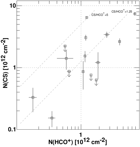
Figure 12: CS and $\mathrm{HCO^{+}}$ column densities measured in absorption, see Appendix C

References

- Berné et al. (2010) Berné, O., Marcelino, N., & Cernicharo, J. 2010, Nature, 466, 947
- Bialy et al. (2019) Bialy, S., Neufeld, D., Wolfire, M., Sternberg, A., & Burkhart, B. 2019, ApJ, 885, 109
- Bigiel et al. (2015) Bigiel, F., Leroy, A. K., Blitz, L., et al. 2015, ApJ, 815, 103
- Boger & Sternberg (2006) Boger, G. I., & Sternberg, A. 2006, ApJ, 645, 314
- Bolatto et al. (2013) Bolatto, A. D., Wolfire, M., & Leroy, A. K. 2013, ARA&A, 51, 207
- Burton & Gordon (1978) Burton, W. B., & Gordon, M. A. 1978, A&A, 63, 7
- Charnley & Markwick (2003) Charnley, S. B., & Markwick, A. J. 2003, A&A, 399, 583
- Dame et al. (2001) Dame, T. M., Hartmann, D., & Thaddeus, P. 2001, ApJ, 547, 792
- Draine (2011) Draine, B. T. 2011, Physics of the Interstellar and Intergalactic Medium (Princeton University Press, 2011. ISBN: 978-0-691-12214-4)
- Dufour & Charnley (2019) Dufour, G., & Charnley, S. B. 2019, ApJ, 887, 67
- Gerin et al. (1997) Gerin, M., Falgarone, E., Joulain, K., et al. 1997, A&A, 318, 579
- Godard et al. (2014) Godard, B., Falgarone, E., & Pineau des Forêts, G. 2014, A&A, 570, A27
- Goldreich & Kwan (1974) Goldreich, P., & Kwan, J. 1974, ApJ, 189, 441
- Goldsmith et al. (2008) Goldsmith, P. F., Heyer, M., Narayanan, G., et al. 2008, ApJ, 680, 428
- Grenier et al. (2005) Grenier, I. A., Casandjian, J.-M., & Terrier, R. 2005, Science, 307, 1292
- Helfer & Blitz (1997) Helfer, T. T., & Blitz, L. 1997, ApJ, 478, 233
- Hensley & Draine (2017) Hensley, B. S., & Draine, B. T. 2017, ApJ, 836, 179
- Heyer et al. (2016) Heyer, M., Goldsmith, P. F., Yıldız, U. A., et al. 2016, MNRAS, 461, 3918
- Jiménez-Donaire et al. (2017) Jiménez-Donaire, M. J., Cormier, D., Bigiel, F., et al. 2017, ApJ, 836, L29
- Jiménez-Donaire et al. (2019) Jiménez-Donaire, M. J., Bigiel, F., Leroy, A. K., et al. 2019, ApJ, 880, 127
- Le Bourlot et al. (1993) Le Bourlot, J., Pineau des Forets, G., Roueff, E., & Schilke, P. 1993, ApJ, 416, L87
- Le Petit et al. (2002) Le Petit, F., Roueff, E., & Le Bourlot, J. 2002, A&A, 390, 369
- Lee et al. (1998) Lee, H.-H., Roueff, E., Pineau des Forets, G., et al. 1998, A&A, 334, 1047
- Liszt (2014a) Liszt, H. 2014a, ApJ, 783, 17
- Liszt (2014b) —. 2014b, ApJ, 780, 10
- Liszt et al. (2018) Liszt, H., Gerin, M., & Grenier, I. 2018, A&A, 617, A54
- Liszt et al. (2019) —. 2019, A&A, 627, A95
- Liszt & Lucas (2001) Liszt, H., & Lucas, R. 2001, A&A, 370, 576
- Liszt et al. (2012) Liszt, H., Sonnentrucker, P., Cordiner, M., & Gerin, M. 2012, ApJ, 753, L28
- Liszt (1995) Liszt, H. S. 1995, ApJ, 442, 163
- Liszt (1997) —. 1997, A&A, 322, 962
- Liszt (2007) —. 2007, A&A, 476, 291
- Liszt (2008) —. 2008, A&A, 492, 743
- Liszt (2011) —. 2011, A&A, 527, A45
- Liszt (2012) —. 2012, A&A, 538, A27
- Liszt (2015) —. 2015, ApJ, 799, 66
- Liszt (2017) —. 2017, ApJ, 835, 138
- Liszt et al. (1984) Liszt, H. S., Burton, W. B., & Xiang, D.-L. 1984, A&A, 140, 303
- Liszt & Gerin (2016) Liszt, H. S., & Gerin, M. 2016, A&A, 585, A80
- Liszt & Lucas (1998) Liszt, H. S., & Lucas, R. 1998, A&A, 339, 561
- Liszt & Pety (2012) Liszt, H. S., & Pety, J. 2012, A&A, 541, A58
- Liszt & Pety (2016) —. 2016, ApJ, 823, 124
- Liszt et al. (2010) Liszt, H. S., Pety, J., & Lucas, R. 2010, A&A, 518, A45+
- Liszt et al. (2009) Liszt, H. S., Pety, J., & Tachihara, K. 2009, A&A, 499, 503
- Lucas & Liszt (1996) Lucas, R., & Liszt, H. S. 1996, A&A, 307, 237
- Lucas & Liszt (2000) —. 2000, A&A, 358, 1069
- Lucas & Liszt (2002) —. 2002, A&A, 384, 1054
- Magnani et al. (1985) Magnani, L., Blitz, L., & Mundy, L. 1985, ApJ, 295, 402
- Mount et al. (2012) Mount, B. J., Redshaw, M., & Myers, E. G. 2012, PhRvA, 85, 012519
- Planck Collaboration et al. (2015) Planck Collaboration, Fermi Collaboration, Ade, P. A. R., et al. 2015, A&A, 582, A31
- Roman-Duval et al. (2016) Roman-Duval, J., Heyer, M., Brunt, C. M., et al. 2016, ApJ, 818, 144
- Roueff et al. (2015) Roueff, E., Loison, J. C., & Hickson, K. M. 2015, A&A, 576, A99
- Schlegel et al. (1998) Schlegel, D. J., Finkbeiner, D. P., & Davis, M. 1998, ApJ, 500, 525
- Shetty et al. (2011) Shetty, R., Glover, S. C., Dullemond, C. P., & Klessen, R. S. 2011, MNRAS, 412, 1686
- Shirley (2015) Shirley, Y. L. 2015, Publ. Astron. Soc. Pac., 127, 299
- Sofia et al. (2004) Sofia, U. J., Lauroesch, J. T., Meyer, D. M., & Cartledge, S. I. B. 2004, ApJ, 605, 272
- Szucs et al. (2016) Szucs, L., Glover, S. C. O., & Klessen, R. S. 2016, MNRAS, 460, 82
- Tritsis et al. (2018) Tritsis, A., Federrath, C., Schneider, N., & Tassis, K. 2018, MNRAS, 481, 5275
- Valdivia et al. (2017) Valdivia, V., Godard, B., Hennebelle, P., et al. 2017, A&A, 600, A114
- Wakelam et al. (2006) Wakelam, V., Herbst, E., Selsis, F., & Massacrier, G. 2006, A&A, 459, 813
- Wolfire et al. (2010) Wolfire, M. G., Hollenbach, D., & McKee, C. F. 2010, ApJ, 716, 1191
- Wolfire et al. (1995) Wolfire, M. G., Hollenbach, D., McKee, C. F., Tielens, A. G. G. M., & Bakes, E. L. O. 1995, ApJ, 443, 152
- Wolfire et al. (2003) Wolfire, M. G., McKee, C. F., Hollenbach, D., & Tielens, A. G. G. M. 2003, ApJ, 587, 278
- Wouterloot et al. (2008) Wouterloot, J. G. A., Henkel, C., Brand, J., & Davis, G. R. 2008, A&A, 487, 237
- Zucker et al. (2019) Zucker, C., Speagle, J. S., Schlafly, E. F., et al. 2019, ApJ, 879, 125