Sparsity-based audio declipping methods: selected overview, new algorithms, and large-scale evaluation

Abstract

Recent advances in audio declipping have substantially improved the state of the art. Yet, practitioners need guidelines to choose a method, and while existing benchmarks have been instrumental in advancing the field, larger-scale experiments are needed to guide such choices. First, we show that the clipping levels in existing small-scale benchmarks are moderate and call for benchmarks with more perceptually significant clipping levels. We then propose a general algorithmic framework for declipping that covers existing and new combinations of variants of state-of-the-art techniques exploiting time-frequency sparsity: synthesis vs. analysis sparsity, with plain or structured sparsity. Finally, we systematically compare these combinations and a selection of state-of-the-art methods. Using a large-scale numerical benchmark and a smaller scale formal listening test, we provide guidelines for various clipping levels, both for speech and various musical genres. The code is made publicly available for the purpose of reproducible research and benchmarking.

I Introduction

Clipping, also known as saturation, is a common phenomenon that can arise from hardware or software limitations in any audio acquisition pipeline. It results in severely distorted audio recordings. Magnitude saturation can occur at different steps in the acquisition, reproduction or Analog-to-Digital Conversion (ADC) process. Restoring a saturated signal is of great interest for many applications in digital communications, image processing or audio. In the latter, while light to moderate clipping causes only some audible clicks and pops, more severe saturation highly affects the sound quality, contaminating it with rattle noise and distortion. The perceived degradation depends on the clipping threshold and the original signal, and it can lead to significant loss in perceived audio quality [1]. More recently, studies [2, 3] also showed the negative impact of clipped signals when used in signal processing pipelines for recognition, transcription or classification.

The idealized hard-clipping model is a simple yet accurate approximation of the magnitude saturation phenomenon and allows to easily identify the clipped and reliable samples. Denoting $\boldsymbol{\mathbf{{x}}}\in\mathbb{R}^{\mathsf{L}}$ a clean original discrete signal, a clipped version $\boldsymbol{\mathbf{{y}}}\in\mathbb{R}^{\mathsf{L}}$ is modeled as follows:

$$\boldsymbol{\mathbf{{y}}}_{\mathrm{i}}=\left\{\begin{array}[]{l l}\boldsymbol{\mathbf{{x}}}_{\mathrm{i}}&\quad\text{when }|\boldsymbol{\mathbf{{x}}}_{\mathrm{i}}|\leq\tau;\\ \operatorname*{sgn\,}(\boldsymbol{\mathbf{{x}}}_{\mathrm{i}})\tau&\quad\text{otherwise;}\\ \end{array}\right.$$ (1)

with $\boldsymbol{\mathbf{{y}}}_{\mathrm{i}}$ (resp. $\boldsymbol{\mathbf{{x}}}_{\mathrm{i}}$) denotes $\mathrm{i}$^th sample from $\boldsymbol{\mathbf{{y}}}$ (resp. $\boldsymbol{\mathbf{{x}}}$) and $\tau$ the hard-clipping threshold. This is illustrated in Figure 1. In the hard-clipping model, which corresponds for example to digital clipping at the ADC level, it is easy to locate the clipped segments and this is an information used by most state-of-the-art declipping methods. In real settings where softer saturation occurs, locating the clipped segments is less straightforward, and dedicated methods, such as [4], could be used for clipping detection.

Figure 1: Hard-clipping model (1)

The terms declipping and desaturation are equally employed to denote the tentative inversion of this process, aiming at restoring the original signal $\boldsymbol{\mathbf{{x}}}$ in its full dynamics and quality, from the sole knowledge of its degraded version $\boldsymbol{\mathbf{{y}}}$. This task has gained a lot of attention in the last decade, as effective approaches based on sparse regularization techniques flourished [5, 3, 6, 7]. After this accumulation of progress, the domain now seems mature enough to address much more severe levels of degradation than those considered in early work. Such an ambition is indeed crucial because real-world applications require to consider such ranges where saturation is prominently audible, as we will show later.

In parallel, limited steps have been made towards evaluation on a common data set. Comparisons have been made possible to some extent by the use of sound excerpts from the SMALLbox toolbox [8] as experimental material of many works in the field, from the pioneering ones [5, 6] to most recent algorithms [9, 10]. This freely available data set was itself extracted from the SiSEC evaluation campaign [11] and is sometimes referred to as “the SMALL data set”. It includes twenty 5-second excerpts (10 speech, 10 music) sampled at 16 kHz (and ten additional 8 kHz speech excerpts unsuited for declipping applications), with a necessarily limited diversity, although effort has been put to cover various types of audio contents. On the other hand, some other authors gathered their own data [12, 3, 7]. Thus, a large-scale and systematic evaluation of the numerous variants of these algorithms on common data was, to date, still to be accomplished.

In order to carry out the needed systematic and large-scale benchmarking of a representative selection of time-frequency single-channel audio declipping algorithms, this paper introduces a new joint modeling and algorithmic framework, mimicking many existing algorithms and encompassing new combinations of the various ideas introduced by them (sparse and cosparse models, plain or structured sparsity). As a prologue, section II discusses the objective measures of clipping levels, which sheds light on the incompleteness of previous evaluations, and identifies the perceptually relevant clipping levels that real-world applications need to target. After recalling the main ingredients of state-of-the-art algorithms in section III, we present our framework in section IV and show how it allows i) to mimic existing algorithms, ii) to formulate new combinations and iii) to handily conduct systematic experiments. The versatility of the framework is illustrated in section V on small-scale and large-scale experiments, evaluated with signal-based objective performance measures, perceptually-motivated objective quality measures, and a listening test. From these experiments, in the final section, we contribute guidelines for declipping practice and evaluation methodology, together with ideas on future research.

II How to quantify clipping?

Quantifying the consequence of clipping can be itself an interesting problem. Even looking at the degradation from a signal perspective only can lead to various interpretations whether one focuses on the clipping threshold, the distortion or the amount of affected samples. In the following, we compare these usual clipping level indexes and provide clipping scales where perceptual differences are of interest.

II-A Signal-based objectives measures of saturation

Commonly [5, 3, 6, 7], clipping is directly rated from the clipping threshold ($\tau$ on Figure 1) as it reflects how strongly the dynamic range of the signal is affected. The lower $\tau$, the more severe the degradation. Practically, studies usually work with normalized magnitude data for fair comparisons, and the clipping threshold takes values in $[0;1]$. This value, which we term clipping threshold is also referred to as “clipping level”.

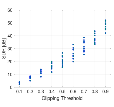
(a) $\tau$ vs. SDR

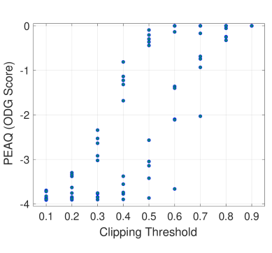
(b) $\tau$ vs. PEAQ

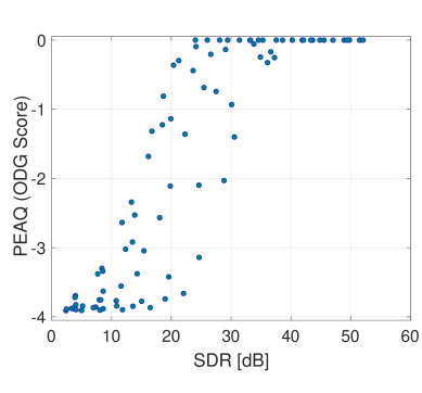
(c) SDR vs. PEAQ

Figure 2: Clipping measures comparisons (SMALLbox music examples)

Another tool to quantify clipping is the relative level of distortion, measured by the Signal-to-Distortion Ratio in decibels:

$$\text{SDR}=10\cdot\log_{10}\left(\frac{\|\boldsymbol{\mathbf{{x}}}\|_{2}^{2}}{\|\boldsymbol{\mathbf{{x}}}-\boldsymbol{\mathbf{{y}}}\|_{2}^{2}}\right).$$ (2)

Contrary to the clipping threshold $\tau$, the SDR is highly linked to the content of the initial signal $\boldsymbol{\mathbf{{x}}}$ as its computation takes into account the energy of the signal.

In the limit case where the signal is not distorted at all, $\boldsymbol{\mathbf{{y}}}=\boldsymbol{\mathbf{{x}}}$ and the SDR tends to its maximum value $+\infty$ dB. In the other extreme case, when the clipping threshold $\tau$ tends to zero, $\boldsymbol{\mathbf{{y}}}$ tends to an all-zero vector and only retains the sign of the samples of $\boldsymbol{\mathbf{{x}}}$. In this limit, the energy of the induced distortion $\|\boldsymbol{\mathbf{{x}}}-\boldsymbol{\mathbf{{y}}}\|_{2}^{2}$ is as large as the initial signal energy $\|\boldsymbol{\mathbf{{x}}}\|_{2}^{2}$ and the SDR tends to its minimum value $0$ dB.

In order to evaluate the SDR, one needs the original clean signal, while determining the clipping threshold requires knowing the initial dynamic range. There exists also a mean to estimate the seriousness of the degradation without any reference: by counting the “proportion” of a signal that is affected by clipping. In a discrete setting, this boils down to counting the proportion of clipped samples over the complete signal. This “ratio of clipped samples” can be denoted

$$\%_{\text{Clipped}}=\frac{|\{\mathrm{i}\in(1,...,\mathsf{L}_{\textrm{total}})\leavevmode\nobreak\ \mid\leavevmode\nobreak\ |\boldsymbol{\mathbf{{x}}}_{\mathrm{i}}|\geq\tau\}|}{\mathsf{L}_{\textrm{total}}}\cdot 100,$$ (3)

where here $\mathsf{L}_{\textrm{total}}$ denotes the total number of samples. The higher this ratio, the more significant will be the loss as more samples are affected. Even if this measure can be of great interest to blindly estimate the power of the degradation, it is rarely used in studies, as it is not suited for direct comparisons or assessing enhancement.

II-B Perceptually-motivated objective quality measures

As for every study involving audio content, numerical indexes used to rate a degradation are relevant if they correlate somehow to perceptual quality ratings obtained via listening tests. Unlike denoising, few studies have focused on finding objective numerical descriptors to rate the quality of saturated audio excerpts. Some years ago, [14] validated the correlation between PEAQ scores [15] and clipped audio quality assessments by using listening tests. In the following, we will briefly investigate the relationship between clipping thresholds, SDR, PEAQ for music and MOS-PESQ [16] for speech to identify a degradation range of interest. These preliminary comparisons are held on the SMALL examples. Let us recall that PEAQ scores are adapted to music excerpts and ranges from $-4$ to $0$. The closer the value is to $-4$, the more annoying the clipping consequences will be perceived. PESQ scores for speech excerpts range from $1$ (bad quality) to $5$ (excellent quality).

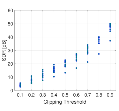
(a) $\tau$ vs. SDR

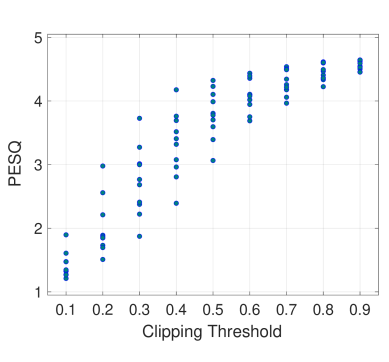
(b) $\tau$ vs. PESQ

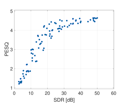
(c) SDR vs. PESQ

Figure 3: Clipping measures comparisons (SMALLbox speech examples)

II-C Perceptual relevance: clipping threshold vs. SDR

Considering what signal-based objective quality measure should be used to describe the strength of the degradation caused by clipping, two main options are available: i) clipping threshold or SDR if a reference signal is available; ii) ratio of clipped samples otherwise. Since we focus in this paper on benchmarking declipping methods in a controlled setting, it is natural to focus on the first option.

As could be expected, and as shown in Figure 2a and Figure 3a on the SMALL data set, the SDR is overall an increasing function of the clipping threshold. Yet, it remains highly variable as a function of the audio content and its temporal structure. Indeed, for a given clipping threshold, a signal with high dynamic will lose a limited number of samples, while more samples will be clipped in a signal whose magnitude values are more uniformly distributed.

To compare the perceptual relevance of the clipping threshold and the SDR, Figure 2b and Figure 2c (resp. Figure 3b and Figure 3c) display the PEAQ (resp. PESQ) perceptually-motivated objective quality measure as a function of these two criteria, on SMALL music (resp. speech) examples, artificially hard-clipped with clipping thresholds between 0.1 and 0.9. As expected, for both speech and music, the estimated rated quality overall increases with the clipping threshold and with the SDR. However, as can be observed in Figure 2b and Figure 3b, both PEAQ and PESQ values are highly variable for a given clipping threshold, except for the most extreme values. What is even more striking for music is that quality, as measured by PEAQ, stabilizes around its maximum (imperceptible degradation) when the SDR roughly exceeds 30 dB. To some extent, a similar behaviour is observed for PESQ values on speech. One should be aware that SDR also has weaknesses. Particularly, highly dynamic signals, comprising very short, high-magnitude segments, would score a lower SDR, yet such degradations may not seriously affect the perceived audio quality. Nonetheless, in such a case, the clipping threshold measure would perform poorly as well. All this suggests to focus on the SDR rather than the clipping threshold as a primary measure of the clipping level of the initial signal.

II-D Perceptually relevant degradation ranges

In light of Figure 2a, it appears that most of the SMALL music examples with clipping threshold above $0.6$ correspond to an SDR of $30$ dB or more, corresponding to potentially imperceptible degradation. Moreover, as the state of the art in audio declipping shows great potential for the restoration of highly degraded signals, it becomes desirable to focus on test cases involving initial SDRs below $30$ dB.

III Prior work on sparse audio declipping

First attempts to address declipping, e.g., with autoregressive models, can be traced back to several decades [17]. Significant progress towards efficient declipping was made in the last ten years by combining ideas from inverse problems and sparse regularization. Each of the following subsections described the main ingredients associated to each of these ideas, which encompass the expression of declipping as a linear inverse problem, exploiting consistency constraints, and the use of sparse and structured time-frequency models under different variants (analysis or synthesis). Existing sparse audio declipping methods often combine one or more of these ideas.

III-A Declipping as a linear inverse problem

The declipping problem can be cast as an underdetermined, linear inverse problem, akin to so-called inpainting [5]. It can be addressed by means of sparse regularization in the time-frequency domain using, e.g., a two-stage algorithm based on Orthogonal Matching Pursuit (OMP) [5]. In a first stage, the active time-frequency atoms of the sparse representation are greedily identified using OMP on the “reliable” samples of the signal (i.e., the samples which have been observed without clipping, cf. Eq. (1)). Then, a declipping constraint is imposed in the transformed domain so the name Constrained Orthogonal Matching Pursuit. Besides such greedy algorithms, lines of work involving convex optimization have been investigated, e.g., using ${\ell_{1}}$-norm minimization and a perceptually oriented sparse representation to perform the reconstruction [14], or ${\ell_{2}}$-norm regularization for alleviating the effect of clipping in automated speech recognition [3]. More recently, a method based on linearly or quadratically constrained weighted least-squares was introduced [18] to tackle a relaxed version of declipping (compression, or soft-clipping, compensation).

III-B Consistency constraint

Besides the exploitation of time-frequency sparsity (see below), a crucial step to improve the efficiency of declipping was the incorporation of the full clipping model (1) within the iterations of the sparse regularization algorithm [12]. The so-called clipping consistency constraint aims at doing so, by making sure that the reliable (non-clipped) parts of the observed (clipped) signal exactly match those of the reconstructed signal. At the same time, clipping consistency also ensures that the magnitudes of the reconstructed samples (corresponding to the clipped samples of the original signal) exceed the clipping threshold, with the appropriate sign. While this idea was already present in [5] (but only as a final step), all state-of-the-art declipping methods now apply the consistency constraint at each iteration. This strategy was shown to drastically improve reconstruction performance. Technical details on techniques to enforce such consistency constraints will be given in Section IV.

III-C Sparse & structured time-frequency signal models

In parallel, a shift from a (now) traditional sparse synthesis approach to sparse analysis was proposed [19], as well as some model refinements exploiting notions of structured sparsity, especially that of social sparsity [20] in the time-frequency domain [6].

III-C1 Plain sparsity, analysis vs. synthesis

The sparse synthesis model assumes that the signal of interest $\boldsymbol{\mathbf{{x}}}$ is built from a linear combination of atoms aggregated in a large dictionary $\boldsymbol{\mathbf{{D}}}$. We could more precisely write

$$\boldsymbol{\mathbf{{x}}}=\boldsymbol{\mathbf{{D}}}\boldsymbol{\mathbf{{z}}}$$ (4)

with $\boldsymbol{\mathbf{{x}}}\in\mathbb{R}^{\mathsf{L}}$ the time domain signal (or a windowed frame extracted from this signal), $\boldsymbol{\mathbf{{D}}}\in{\mathbb{C}^{\mathsf{\mathsf{L}\times\mathsf{S}}}}$ the dictionary and $\boldsymbol{\mathbf{{z}}}\in\mathbb{C}^{\mathsf{S}}$ a sparse representation of the vector $\boldsymbol{\mathbf{{x}}}$ ($\mathsf{S}\geq\mathsf{L}$). This models considers that $\|\boldsymbol{\mathbf{{z}}}\|_{0}$, the number of non-zero coefficients in $\boldsymbol{\mathbf{{z}}}$, is very small compared to the size $\mathsf{S}$ of the vector. In other words, one needs very few atoms of $\boldsymbol{\mathbf{{D}}}$ to synthesize $\boldsymbol{\mathbf{{x}}}$ from $\boldsymbol{\mathbf{{z}}}$.

While synthesis approaches comprise a vast majority of the sparsity-based time-frequency regularization techniques, it has been demonstrated in [21] and more recently in [22, 19] that the analysis sparse model, also known as the cosparse model, can turn out to be advantageous in certain settings, in particular in terms of computational cost. Instead of implicitly defining a sparse representation $\boldsymbol{\mathbf{{z}}}$ of the signal $\boldsymbol{\mathbf{{x}}}$ through the sparse synthesis model $\boldsymbol{\mathbf{{x}}}=\boldsymbol{\mathbf{{D}}}\boldsymbol{\mathbf{{z}}}$, the rationale of the cosparse model is to explicitly assume that

$$\boldsymbol{\mathbf{{z}}}=\boldsymbol{\mathbf{{A}}}\boldsymbol{\mathbf{{x}}}$$ (5)

is sparse, where $\boldsymbol{\mathbf{{A}}}\in{\mathbb{C}^{\mathsf{\mathsf{P}\times\mathsf{L}}}}$ is called the analysis operator ($\mathsf{P}\geq\mathsf{L}$). Models are equivalent when $\mathsf{P}=\mathsf{S}=\mathsf{L}$ and $\boldsymbol{\mathbf{{A}}}\boldsymbol{\mathbf{{D}}}=\boldsymbol{\mathbf{{I}}}$.

III-C2 Structured (co)sparse time-frequency models

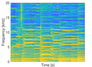
(a) Tonal music

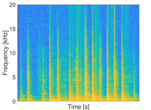
(b) Percussive sounds

Figure 4: Short Time Fourier Transform magnitude of two music signals

Plain synthesis sparse models as defined in (4) somehow assume that each coefficient in the sparse representation can be active or inactive independently from the others. However, in the context of audio time-frequency modeling one can argue that coefficients are rather arranged in groups as shown in Figure 4. In a tonal musical excerpt (Figure 4a) high energy coefficients are structured across time in the spectrogram, reflecting the strong presence of harmonics; in a percussive music sample spectrogram (Figure 4b), the dominant coefficients gather across frequency due to transients and beats. Structured forms of sparsity such as group sparsity [23, 24] or social sparsity [25, 20] have emerged as useful refinements to take into account such typical time-frequency patterns of audio signals.

Consider the matrix $\boldsymbol{\mathbf{{X}}}\in{\mathbb{R}^{\mathsf{\mathsf{L}\times\mathsf{G}}}}$ which columns are the windowed frames of an original time-domain audio signal and $\boldsymbol{\mathbf{{Z}}}\in{\mathbb{C}^{\mathsf{\mathsf{S}\times\mathsf{G}}}}$ a matrix which columns are a frequency representation of these frames. In other words, this matrix is a time-frequency representation of the underlying audio signal. In structured sparse models, the assumed relation between $\boldsymbol{\mathbf{{Z}}}$ and $\boldsymbol{\mathbf{{X}}}$ becomes:

Structured analysis model	Structured synthesis model
$\boldsymbol{\mathbf{{A}}}\in{\mathbb{C}^{\mathsf{\mathsf{P}\times\mathsf{L}}}},\mathsf{P}\geq\mathsf{L}$	$\boldsymbol{\mathbf{{D}}}\in{\mathbb{C}^{\mathsf{\mathsf{L}\times\mathsf{S}}}},\mathsf{S}\geq\mathsf{L}$
$\boldsymbol{\mathbf{{Z}}}\simeq\boldsymbol{\mathbf{{A}}}\boldsymbol{\mathbf{{X}}},\boldsymbol{\mathbf{{Z}}}\in{\mathbb{C}^{\mathsf{\mathsf{P}\times\mathsf{G}}}}$	$\boldsymbol{\mathbf{{D}}}\boldsymbol{\mathbf{{Z}}}\simeq\boldsymbol{\mathbf{{X}}},\boldsymbol{\mathbf{{Z}}}\in{\mathbb{C}^{\mathsf{\mathsf{S}\times\mathsf{G}}}}$
$\|\boldsymbol{\mathbf{{Z}}}\|_{0}\ll\mathsf{P}\times\mathsf{G}$	$\|\boldsymbol{\mathbf{{Z}}}\|_{0}\ll\mathsf{S}\times\mathsf{G}$
$\boldsymbol{\mathbf{{Z}}}$ is “structured”;	$\boldsymbol{\mathbf{{Z}}}$ is “structured”.

Considering non-overlapping groups of indexes in $\boldsymbol{\mathbf{{Z}}}$, group sparsity assumes that if some coefficient of the matrix is zero, then all coefficients at indexes belonging to the same group must be also zero, while in “active” groups, no sparsity is required. This prior is typically enforced by expressing optimization problems involving mixed-norms such as the ${\ell_{{2},{1}}}$ norm [26]. Optimization algorithms to address such minimization problems typically involve structured thresholding operators. Social sparsity extends group sparsity to the case of possibly overlapping groups, and also allows more flexible structures through the use of generic time-frequency patterns. This prior is typically enforced in iterative algorithms with the use of appropriate specific sparsity-promoting operators using dependencies between coefficients.

IV Proposed approach

In this section, we present a general framework using either simple sparse modeling (analysis or synthesis based) or structured sparse priors to address the audio declipping problem. Given a matrix $\boldsymbol{\mathbf{{Y}}}\in{\mathbb{R}^{\mathsf{\mathsf{L}\times\mathsf{G}}}}$ whose columns are the windowed frames of a clipped time-domain audio signal $\boldsymbol{\mathbf{{y}}}$, our goal is to recover an estimate $\hat{\boldsymbol{\mathbf{{X}}}}$ of the frames $\boldsymbol{\mathbf{{X}}}$ of the original signal. To this end, one seeks $\hat{\boldsymbol{\mathbf{{X}}}}$ satisfying:

• the modeling constraints described in subsection III-C;

• a data fidelity constraint with respect to $\boldsymbol{\mathbf{{Y}}}$, according to some distortion model (clipping).

This is the spirit of the algorithmic framework we develop. It relies on two components:

• a shrinkage enforcing (structured) sparsity;

• a generalized projection onto the clipping-consistent data-fidelity constraint.

Before further describing these components in the rest of this section, we formalize some notational conventions. In the following, lower-case Greek symbols ($\varepsilon$) stands for scalar constant. Lower-case sans serif font ($\mathsf{i}$) denotes an integer. Lower-case bold font ($\boldsymbol{\mathbf{{v}}}$) expresses a vector and upper-case ($\boldsymbol{\mathbf{{V}}}$) a matrix. $\boldsymbol{\mathbf{{v}}}_{\mathsf{i}}$ is an $\mathsf{i}$^th element of a vector and $\boldsymbol{\mathbf{{v}}}^{\mathsf{(i)}}$ an $\mathsf{i}$^th iterate. $\Theta$ is used for a set. $\mathcal{O}$ stands for a non-linear operator and $F$ a function. $\boldsymbol{\mathbf{{V}}}_{\mathsf{i}\mathsf{j}}$ represents the component of the matrix $\boldsymbol{\mathbf{{V}}}$ indexed the $\mathsf{i}$^th row and $\mathsf{j}$^th column. Finally, $\boldsymbol{\mathbf{{V}}}^{\mathsf{H}}$ denotes the Hermitian transpose of a matrix $\boldsymbol{\mathbf{{V}}}$. Curved relation symbols ($\preccurlyeq,\succcurlyeq,\prec,\succ$) are used for entry-wise comparisons between matrices. Other notations will be disambiguated in the text.

IV-A Sparsity-promoting shrinkage operators

Shrinkage operators, also known as “thresholding rules” [27], promote sparsity by reducing the magnitude of their input and possibly setting it to zero.

Definition 1 (Shrinkage).

$\mathcal{S}(\cdot)$, is a shrinkage if:

1. $\mathcal{S}(\cdot)$ is an odd function;

2. $0\leq\mathcal{S}(x)\leq x$, for all $x\in\mathbb{R}^{+}$.

3. $(\mathcal{S}(\cdot))_{+}$ is nondecreasing on $\mathbb{R}^{+}$ and $\lim_{x\rightarrow+\infty}(\mathcal{S}(x))_{+}=+\infty$, where $(\cdot)_{+}:=\max(\cdot,0)$.

When applied to a (time-frequency) matrix, and written $\mathcal{S}(\boldsymbol{\mathbf{{Z}}})$, shrinkage is applied entry-wise. Different shrinkage operators have been proposed depending on the sparse prior to account for (i.e., plain or structured sparsity). These shrinkage operators are presented below.

Plain sparsity

The hard-thresholding operator (HT) $\mathcal{H}_{\mathsf{k}}(\boldsymbol{\mathbf{{Z}}})$ preserves the $\mathsf{k}$ coefficients of largest magnitude in $\boldsymbol{\mathbf{{Z}}}$ and sets the other ones to zero [28]. It can be used to enforce plain time-frequency sparsity, either analysis or synthesis.

Social (time-frequency) sparsity

The Persistent Empirical Wiener (PEW) operator [29, 27] was successfully used in [6] for audio declipping using (synthesis) social sparsity. This shrinkage promotes specific local time-frequency patterns around each time-frequency point. Its specification explicitly requires choosing a time-frequency pattern described as a matrix $\Gamma\in{\mathbb{R}^{\mathsf{\mathsf{(\mathsf{2F+1})}\times\mathsf{(\mathsf{2T+1})}}}}$, typically with binary entries. Rows of $\Gamma$ account for the frequency dimension and columns for the time dimension, in local time-frequency coordinates. Let $\boldsymbol{\mathbf{{Z}}}$ be a time-frequency representation. As illustrated on Figure 5, consider $\mathsf{ft}$ the coordinates of a time-frequency point in $\boldsymbol{\mathbf{{Z}}}$ ($\mathsf{f}$ is a frequency index, $\mathsf{t}$ the index of a windowed frame) and $\boldsymbol{\mathbf{{P}}}_{\mathsf{ft}}:=[\mathsf{f}-\mathsf{F},\mathsf{f}+\mathsf{F}]\times[\mathsf{t}-\mathsf{T},\mathsf{t}+\mathsf{T}]$ the indices corresponding to a time-frequency patch of size $(\mathsf{2F+1})\times(\mathsf{2W+1})$ centered at time-frame $\mathsf{t}$ and frequency $\mathsf{f}$. The matrix $\boldsymbol{\mathbf{{Z}}}_{\boldsymbol{\mathbf{{P}}}_{\mathsf{ft}}}\in{\mathbb{C}^{\mathsf{\mathsf{(\mathsf{2F+1})}\times\mathsf{(\mathsf{2W+1})}}}}$ is extracted from $\boldsymbol{\mathbf{{Z}}}$ on these indices, with mirror-padding on the borders if needed.

Figure 5: Schematic representation of patch extraction from matrix $\boldsymbol{\mathbf{{Z}}}$

Now, given a thresholding parameter $\mu\geq 0$, we can define the PEW shrinkage operator $\mathcal{S}^{\text{PEW}}_{\mu}$. Denoting $\circ$ the (Hadamard) entrywise product and $(\cdot)_{+}=\max(\cdot,0)$ the positive part:

$$\mathcal{S}^{\text{PEW}}_{\mu}(\boldsymbol{\mathbf{{Z}}}|\Gamma)_{\mathsf{ft}}:=\boldsymbol{\mathbf{{Z}}}_{\mathsf{ft}}\cdot\left(1-\frac{\mu^{2}}{\|\boldsymbol{\mathbf{{Z}}}_{\boldsymbol{\mathbf{{P}}}_{\mathsf{ft}}}\circ\Gamma\|_{\text{F}}^{2}}\right)_{+}.$$ (6)

Since $\|\boldsymbol{\mathbf{{Z}}}_{\boldsymbol{\mathbf{{P}}}_{\mathsf{ft}}}\circ\Gamma\|_{\text{F}}^{2}$ is the energy of $\boldsymbol{\mathbf{{Z}}}$ restricted to a time-frequency neighborhood of $\mathsf{ft}$ of shape specified by $\Gamma$, the left hand side is zero as soon as this energy falls below $\mu^{2}$. As such, PEW shrinkage effectively promotes structured sparsity.

Remark.

To use similar notations for plain and social sparsity, in the case of analysis (resp. synthesis) plain sparse modeling with $\boldsymbol{\mathbf{{A}}}\in{\mathbb{C}^{\mathsf{\mathsf{P}\times\mathsf{L}}}}$ a forward frequency analysis operator (resp. $\boldsymbol{\mathbf{{D}}}\in{\mathbb{C}^{\mathsf{\mathsf{L}\times\mathsf{S}}}}$ a dictionary) we denote $\mathcal{S}_{\mu}:=\mathcal{H}_{\mathsf{P}-\mu}$ (resp. $\mathcal{S}_{\mu}:=\mathcal{H}_{\mathsf{S}-\mu}$), for $\mu\in\mathbb{N}^{+}$, $0\leq\mu\leq\mathsf{P}$ (resp. $0\leq\mu\leq\mathsf{S}$). Hence, the smaller $\mu$, the less thresholding is performed. The large $\mu$, the sparser the result of both $\mathcal{S}_{\mu}(\cdot)$ and $\mathcal{S}^{\text{PEW}}_{\mu}(\cdot|\Gamma)$. In all cases, $\mu$ is thus a parameter controlling the strength of the performed shrinkage, which is stronger when $\mu$ is larger.

Examples of time-frequency patterns $\Gamma$ chosen for music are given in Figure 6 and for speech in Figure 7. The unit associated to individual squares is the time-frequency index of the DFT. In the experimental sections, we will take 64 ms time-frames for music and 32 ms time-frames for speech; the total time span for each pattern $\Gamma$ is 320 ms for music and 96 ms for speech. While similar, the patterns for music and for speech are at different time scales, given the different scales of stationarity in speech and music. The structures of these patterns have various properties: $\Gamma_{\mathsf{1}}$, with a frequency localized and time-spread support, will emphasize tonal content; vice-versa, $\Gamma_{\mathsf{3}}$ will emphasize transients and attacks; $\Gamma_{\mathsf{2}}$ is designed [30] to avoid pre-echo artifacts; patterns $\Gamma_{\mathsf{4}}$ and $\Gamma_{\mathsf{5}}$ are introduced to stress tonal transitions; finally, $\Gamma_{\mathsf{6}}$ can serve as a default pattern when no particular structure is identified.

(a) $\Gamma_{\mathsf{1}}$

(b) $\Gamma_{\mathsf{2}}$

(c) $\Gamma_{\mathsf{3}}$

(d) $\Gamma_{\mathsf{4}}$

(e) $\Gamma_{\mathsf{5}}$

(f) $\Gamma_{\mathsf{6}}$

Figure 6: Extended set of time-frequency neighborhoods used for music

(a) $\Gamma_{\mathsf{1}}$

(b) $\Gamma_{\mathsf{2}}$

(c) $\Gamma_{\mathsf{3}}$

(d) $\Gamma_{\mathsf{4}}$

(e) $\Gamma_{\mathsf{5}}$

(f) $\Gamma_{\mathsf{6}}$

Figure 7: Extended set of time-frequency neighborhoods used for speech

IV-B Clipping-consistent generalized projections

We present below the generalized projection that will be crucial to enforce the clipping-consistent data-fidelity constraint along the iterations of the proposed algorithm family.

Denote $\Omega_{+}$ (resp. $\Omega_{-}$) the collection of indices of the samples in matrix $\boldsymbol{\mathbf{{Y}}}$ affected by positive (resp. negative) magnitude clipping. Similarly denote $\Omega_{r}$ the indices of the reliable samples (not affected by clipping). For any of these sets $\Omega$, given a generic matrix $\boldsymbol{\mathbf{{V}}}$ of the same dimensions as $\boldsymbol{\mathbf{{Y}}}$, define $\boldsymbol{\mathbf{{V}}}_{\Omega}$ the matrix formed by keeping unchanged the entries of $\boldsymbol{\mathbf{{V}}}$ indexed by $\Omega$ and setting the rest to zero.

The set of clipping-consistent time-domain estimates $\boldsymbol{\mathbf{{W}}}$ of $\boldsymbol{\mathbf{{X}}}$ can be expressed for the analysis setting by

$$\Theta_{\textrm{time}}(\boldsymbol{\mathbf{{Y}}}):=\left\{\boldsymbol{\mathbf{{W}}}\ |\begin{array}[]{l}\boldsymbol{\mathbf{{W}}}_{\Omega_{r}}=\boldsymbol{\mathbf{{Y}}}_{\Omega_{r}};\\ \boldsymbol{\mathbf{{W}}}_{\Omega_{+}}\succcurlyeq\boldsymbol{\mathbf{{Y}}}_{\Omega_{+}};\\ \boldsymbol{\mathbf{{W}}}_{\Omega_{-}}\preccurlyeq\boldsymbol{\mathbf{{Y}}}_{\Omega_{-}}.\end{array}\right\}$$

where $\boldsymbol{\mathbf{{W}}}$ is of the same size as $\boldsymbol{\mathbf{{Y}}}$. For the synthesis setting, the set of clipping-consistent time-frequency estimates $\boldsymbol{\mathbf{{W}}}$ of $\boldsymbol{\mathbf{{X}}}$ is defined as

$$\Theta_{\textrm{time-freq}}(\boldsymbol{\mathbf{{Y}}}):=\left\{\boldsymbol{\mathbf{{W}}}\ |\begin{array}[]{l}(\boldsymbol{\mathbf{{D}}}\boldsymbol{\mathbf{{W}}})_{\Omega_{r}}=\boldsymbol{\mathbf{{Y}}}_{\Omega_{r}};\\ (\boldsymbol{\mathbf{{D}}}\boldsymbol{\mathbf{{W}}})_{\Omega_{+}}\succcurlyeq\boldsymbol{\mathbf{{Y}}}_{\Omega_{+}};\\ (\boldsymbol{\mathbf{{D}}}\boldsymbol{\mathbf{{W}}})_{\Omega_{-}}\preccurlyeq\boldsymbol{\mathbf{{Y}}}_{\Omega_{-}}.\end{array}\right\}.$$

Here $\boldsymbol{\mathbf{{W}}}$ is a time-frequency estimate gathering as many frames as in $\boldsymbol{\mathbf{{Y}}}$ and $\mathsf{S}$ frequency points, so that $\boldsymbol{\mathbf{{D}}}\boldsymbol{\mathbf{{W}}}$ is a clipping-consistent time-domain estimate of $\boldsymbol{\mathbf{{X}}}$. These choices hold for both plain and structured versions, and the set $\Theta$ is convex in all cases.

Definition 2 (Generalized projection).

Let $\Theta$ be a nonempty convex set, and $\boldsymbol{\mathbf{{M}}}$ be a full column rank matrix. Given a time-frequency matrix $\boldsymbol{\mathbf{{Z}}}$, we denote $\mathcal{P}_{\Theta,\boldsymbol{\mathbf{{M}}}}(\boldsymbol{\mathbf{{Z}}})$ the (unique) solution of the following optimization problem:

$$\operatorname*{minimize\,}_{\boldsymbol{\mathbf{{W}}}\in\Theta}\|\boldsymbol{\mathbf{{M}}}\boldsymbol{\mathbf{{W}}}-\boldsymbol{\mathbf{{Z}}}\|_{\mathrm{F}}.$$ (7)

In the analysis setting, seeking a clipping consistent time-domain estimate $\boldsymbol{\mathbf{{W}}}$ of $\boldsymbol{\mathbf{{X}}}$ whose time-frequency representation approximates a given $\boldsymbol{\mathbf{{Z}}}$ corresponds to computing $\mathcal{P}_{\texttt{ana}}(\boldsymbol{\mathbf{{Z}}}):=\mathcal{P}_{\Theta,\boldsymbol{\mathbf{{M}}}}(\boldsymbol{\mathbf{{Z}}})$ with $\Theta=\Theta_{\textrm{time}}(\boldsymbol{\mathbf{{Y}}})$ and $\boldsymbol{\mathbf{{M}}}:=\boldsymbol{\mathbf{{A}}}$. Considering an analysis operator $\boldsymbol{\mathbf{{A}}}$ such that $\boldsymbol{\mathbf{{A}}}^{\mathsf{H}}\boldsymbol{\mathbf{{A}}}=\boldsymbol{\mathbf{{I}}}$, minimizing $\|\boldsymbol{\mathbf{{A}}}\boldsymbol{\mathbf{{W}}}-\boldsymbol{\mathbf{{Z}}}\|_{\text{F}}^{2}$ with $\boldsymbol{\mathbf{{W}}}\in\Theta$ is equivalent to

$$\operatorname*{minimize\,}_{\boldsymbol{\mathbf{{W}}}}\|\boldsymbol{\mathbf{{W}}}-\boldsymbol{\mathbf{{A}}}^{\mathsf{H}}\boldsymbol{\mathbf{{Z}}}\|_{\text{F}}^{2}\operatorname*{\,subject\,to\,}\boldsymbol{\mathbf{{W}}}\in\Theta.$$

As the constraint is written component-wise, the desired projection can be expressed accordingly for the $\mathsf{n}$-th sample of the $\mathsf{t}$-th time-frame as:

$$[\mathcal{P}_{\texttt{ana}}(\boldsymbol{\mathbf{{Z}}})]_{\mathsf{nt}}\!=\!\left\{\begin{array}[]{l l}(\boldsymbol{\mathbf{{M}}}^{\mathsf{H}}\boldsymbol{\mathbf{{Z}}})_{\mathsf{nt}}&\!\text{if}\!\left\{\begin{array}[]{l}\mathsf{nt}\in\Omega_{+},(\boldsymbol{\mathbf{{M}}}^{\mathsf{H}}\boldsymbol{\mathbf{{Z}}})_{\mathsf{nt}}\geq\tau;\\ \text{or}\\ \mathsf{nt}\in\Omega_{-},(\boldsymbol{\mathbf{{M}}}^{\mathsf{H}}\boldsymbol{\mathbf{{Z}}})_{\mathsf{nt}}\leq-\tau;\end{array}\right.\\ \boldsymbol{\mathbf{{Y}}}_{\mathsf{nt}}&\text{otherwise.}\\ \end{array}\right.$$

In this case, matrix-vector products with $\boldsymbol{\mathbf{{M}}}^{\mathsf{H}}$ dominate the computational cost of the generalized projection. When this can be done with a fast transform, the analysis variant has low complexity.

For the synthesis case, seeking a clipping consistent time-frequency estimate $\boldsymbol{\mathbf{{W}}}$ of $\boldsymbol{\mathbf{{X}}}$ which is close to a given time-frequency representation $\boldsymbol{\mathbf{{Z}}}$ corresponds to computing $\mathcal{P}_{\texttt{syn}}(\boldsymbol{\mathbf{{Z}}}):=\mathcal{P}_{\Theta,\boldsymbol{\mathbf{{M}}}}(\boldsymbol{\mathbf{{Z}}})$ with $\Theta=\Theta_{\textrm{time-freq}}(\boldsymbol{\mathbf{{Y}}})$ and $\boldsymbol{\mathbf{{M}}}:=\boldsymbol{\mathbf{{I}}}$. Such a projection step can be approximated with a nested iterative procedure [22]. Even if this can help building an efficient projection algorithm, the overall computation cost for the synthesis variant remains substantially higher than the analysis version (making it almost intractable). More recently, a closed-form solution for the declipping projection in the synthesis case was obtained [31] when $\boldsymbol{\mathbf{{D}}}$ is a Parseval tight frame (i.e., $\boldsymbol{\mathbf{{D}}}\boldsymbol{\mathbf{{D}}}^{\mathsf{H}}=\boldsymbol{\mathbf{{I}}}$). As detailed in appendix this projection can then be expressed as:

$$\mathcal{P}_{\texttt{syn}}(\boldsymbol{\mathbf{{Z}}}) =\boldsymbol{\mathbf{{Z}}}-\boldsymbol{\mathbf{{D}}}^{\mathsf{H}}(\boldsymbol{\mathbf{{D}}}\boldsymbol{\mathbf{{Z}}}-\Pi(\boldsymbol{\mathbf{{Z}}})),$$ (8)

with

$$[\Pi(\boldsymbol{\mathbf{{Z}}})]_{\mathsf{nt}}\!=\!\left\{\begin{array}[]{l l}(\boldsymbol{\mathbf{{D}}}\boldsymbol{\mathbf{{Z}}})_{\mathsf{nt}}&\!\text{if}\left\{\begin{array}[]{l}\mathsf{nt}\in\Omega_{+},(\boldsymbol{\mathbf{{D}}}\boldsymbol{\mathbf{{Z}}})_{\mathsf{nt}}\geq\tau;\\ \text{or}\\ \mathsf{nt}\in\Omega_{-},(\boldsymbol{\mathbf{{D}}}\boldsymbol{\mathbf{{Z}}})_{\mathsf{nt}}\leq-\tau;\end{array}\right.\\ \boldsymbol{\mathbf{{Y}}}_{\mathsf{nt}}&\text{otherwise.}\\ \end{array}\right.$$

When fast products with $\boldsymbol{\mathbf{{D}}}$ and $\boldsymbol{\mathbf{{D}}}^{\mathsf{H}}$ can be achieved, the synthesis projection also has low complexity.

IV-C Generic declipping algorithm

A generic algorithm for declipping exploiting sparsity, either in its synthesis or analysis variant, with and without structure, is described in Algorithm 1. It takes as input parameters:

• a convex set $\Theta$ and a matrix $\boldsymbol{\mathbf{{M}}}$ embodying the declipping data fidelity constraint and the domain (time or frequency) in which it is specified;

• a parameterized family of shrinkages $\{\mathcal{S}_{\mu}(\cdot)\}_{\mu}$, where the strength of the shrinkage is controlled by $\mu$: in the extreme cases $\mathcal{S}_{0}(\boldsymbol{\mathbf{{Z}}})=\boldsymbol{\mathbf{{Z}}}$ and $\mathcal{S}_{\infty}(\boldsymbol{\mathbf{{Z}}})=\boldsymbol{\mathbf{{0}}}$;

• a rule $F:\mu\mapsto F(\mu)$ to update the shrinkage strength across iterations, and an initial strength $\mu^{\mathsf{(\mathsf{0})}}$;

• an initial time-frequency estimate $\boldsymbol{\mathbf{{Z}}}^{\mathsf{(0)}}$;

• stopping parameters $\beta$ (a threshold on the relative error) and $\mathsf{i}_{\max}$ (a maximum number of iterations).

Algorithm 1 Generic Algorithm: $\mathcal{G}$

0:  $\Theta,\boldsymbol{\mathbf{{M}}},\{\mathcal{S}_{\mu}(\cdot)\}_{\mu},\mu^{\mathsf{(\mathsf{0})}},F(\cdot),\boldsymbol{\mathbf{{Z}}}^{\mathsf{(0)}},\beta,\mathsf{i}_{\max}$

  Initialization step:

  $\boldsymbol{\mathbf{{U}}}^{\mathsf{(0)}}=\boldsymbol{\mathbf{{0}}}$;

  for $\mathsf{i}=1\text{ to }\mathsf{i}_{\max}$ do

     Projection step on the declipping constraint:

     $\boldsymbol{\mathbf{{W}}}^{\mathsf{(i)}}=\mathcal{P}_{\Theta,\boldsymbol{\mathbf{{M}}}}(\boldsymbol{\mathbf{{Z}}}^{\mathsf{(i-1)}}-\boldsymbol{\mathbf{{U}}}^{\mathsf{(i-1)}})$

     Projection step on the modeling constraint:

     $\boldsymbol{\mathbf{{Z}}}^{\mathsf{(i)}}=\mathcal{S}_{\mu^{\mathsf{(i-1)}}}\left(\boldsymbol{\mathbf{{M}}}\boldsymbol{\mathbf{{W}}}^{\mathsf{(i)}}+\boldsymbol{\mathbf{{U}}}^{\mathsf{(i-1)}}\right)$

     Update step:

     if $\frac{\|\boldsymbol{\mathbf{{M}}}\boldsymbol{\mathbf{{W}}}^{\mathsf{(i)}}-\boldsymbol{\mathbf{{Z}}}^{\mathsf{(i)}}\|_{\text{F}}}{\|\boldsymbol{\mathbf{{M}}}\boldsymbol{\mathbf{{W}}}^{\mathsf{(i)}}\|_{\text{F}}}\leq\beta$ then

        terminate

     else

        $\boldsymbol{\mathbf{{U}}}^{\mathsf{(i)}}=\boldsymbol{\mathbf{{U}}}^{\mathsf{(i-1)}}+\boldsymbol{\mathbf{{M}}}\boldsymbol{\mathbf{{W}}}^{\mathsf{(i)}}-\boldsymbol{\mathbf{{Z}}}^{\mathsf{(i)}}$

        $\mu^{\mathsf{(i)}}=F(\mu^{\mathsf{(i-1)}})$

  return  $\boldsymbol{\mathbf{{W}}}^{\mathsf{(\mathsf{i})}}$ [and optionally $\mu^{\mathsf{(i)}}$, $\boldsymbol{\mathbf{{Z}}}^{\mathsf{(i)}}$]

The notation $\boldsymbol{\mathbf{{Z}}}^{\mathsf{(i)}}$ highlights that the corresponding variable is in any use-case a sparse/structured time-frequency representation. The variable $\boldsymbol{\mathbf{{U}}}^{\mathsf{(i)}}$ is an intermediate time-frequency “residual” variable typical of approaches inspired by ADMM (Alternating Direction Method of Multipliers) [32]. At iteration $\mathsf{i}$, an estimate of $\boldsymbol{\mathbf{{Z}}}$ is $\hat{\boldsymbol{\mathbf{{Z}}}}^{\mathsf{(i)}}:=\boldsymbol{\mathbf{{Z}}}^{\mathsf{(i-1)}}-\boldsymbol{\mathbf{{U}}}^{\mathsf{(i-1)}}$. The interpretation of the other variables is use-case dependent:

• analysis variant: $\boldsymbol{\mathbf{{M}}}:=\boldsymbol{\mathbf{{A}}}$ is the frequency analysis operator; $\boldsymbol{\mathbf{{W}}}^{\mathsf{(i)}}$ is an estimate of the time frames $\boldsymbol{\mathbf{{X}}}$, that satisfies the time-domain data-fidelity constraint $\Theta_{\textrm{time}}(\boldsymbol{\mathbf{{Y}}})$ while being closest to $\hat{\boldsymbol{\mathbf{{Z}}}}^{\mathsf{(i)}}$ in the time-frequency domain; the algorithm outputs a time-domain estimate.

• synthesis variant: $\boldsymbol{\mathbf{{M}}}:=\boldsymbol{\mathbf{{I}}}$; $\boldsymbol{\mathbf{{W}}}^{\mathsf{(i)}}$ is a time-frequency estimate of $\boldsymbol{\mathbf{{Z}}}$; the data-fidelity constraint $\Theta_{\textrm{time-freq}}(\boldsymbol{\mathbf{{Y}}})$ is expressed in the time-frequency domain; the algorithm outputs a time-frequency estimate, from which we get a time-domain estimate by synthesis $\hat{\boldsymbol{\mathbf{{X}}}}:=\boldsymbol{\mathbf{{D}}}\boldsymbol{\mathbf{{W}}}^{\mathsf{(i)}}$ with $\boldsymbol{\mathbf{{D}}}$ the inverse frequency transform operator.

Due to the expression of $\Theta$ respectively in the time domain and the time-frequency domain, the analysis and synthesis variants can have different computational properties as will be further studied. We can summarize Algorithm 1 as a generalized procedure:

$$\mathcal{G}(\Theta,\boldsymbol{\mathbf{{M}}},\{\mathcal{S}_{\mu}\}_{\mu},\mu^{\mathsf{(\mathsf{0})}},F,\boldsymbol{\mathbf{{Z}}}^{\mathsf{(0)}},\beta,\mathsf{i}_{\max}).$$ (9)

For reproducibility, the $\text{Matlab}^{\circledR}\leavevmode\nobreak\$code for all variants of this generic algorithm is available [33] under a BSD-3 licence. Audio examples are also available on the web.

IV-D Plain (co)sparse audio declippers

In practice, the algorithms are built to work on a frame-based manner (see further details at the end of this section). In the plain (co)sparse cases, $\boldsymbol{\mathbf{{Y}}}\in{\mathbb{R}^{\mathsf{\mathsf{L}\times\mathsf{1}}}}$ is a vector corresponding to a single windowed frame extracted from the clipped signal $\boldsymbol{\mathbf{{y}}}$. We instantiate the general algorithm $\mathcal{G}$ (Algorithm 1) by choosing the operators described in Table I. The update rule $F$ for $\mu$ is set to gradually decrease $\mu$ by $1$ at each iteration, starting from $\mu^{\mathsf{(0)}}=\mathsf{P}-1$ for the analysis case (resp. $\mu^{\mathsf{(0)}}=\mathsf{S}-1$ for the synthesis case). This way, we relax the sparse constraint along with the iterations.

Table I: Parameters of Algorithm 1 for the Plain Sparse Declippers

Analysis	Synthesis
$\Theta=\Theta_{\textrm{time}}(\boldsymbol{\mathbf{{Y}}})$	$\Theta=\Theta_{\textrm{time-freq}}(\boldsymbol{\mathbf{{Y}}})$
$\boldsymbol{\mathbf{{M}}}=\boldsymbol{\mathbf{{A}}}\in{\mathbb{C}^{\mathsf{\mathsf{P}\times\mathsf{L}}}},\mathsf{P}\geq\mathsf{L}$	$\boldsymbol{\mathbf{{M}}}=\boldsymbol{\mathbf{{I}}}\in{\mathbb{C}^{\mathsf{\mathsf{L}\times\mathsf{L}}}}$,
$\mathcal{S}_{\mu}(\cdot)=\mathcal{H}_{\mathsf{P}-\mu}(\cdot)$	$\mathcal{S}_{\mu}(\cdot)=\mathcal{H}_{\mathsf{S}-\mu}(\cdot)$,
$\mu^{\mathsf{(0)}}=\mathsf{P}-1$	$\mu^{\mathsf{(0)}}=\mathsf{S}-1$
$F:\mu\mapsto\mu-1$	$F:\mu\mapsto\mu-1$
$\boldsymbol{\mathbf{{Z}}}^{\mathsf{(0)}}=\boldsymbol{\mathbf{{A}}}\boldsymbol{\mathbf{{Y}}},\;\boldsymbol{\mathbf{{A}}}\in{\mathbb{C}^{\mathsf{\mathsf{P}\times\mathsf{L}}}}$	$\boldsymbol{\mathbf{{Z}}}^{\mathsf{(0)}}=\boldsymbol{\mathbf{{D}}}^{\mathsf{H}}\boldsymbol{\mathbf{{Y}}},\;\boldsymbol{\mathbf{{D}}}\in{\mathbb{C}^{\mathsf{\mathsf{L}\times\mathsf{S}}}}$

Iterating Algorithm 1 with the parameters described above gives a declipped estimate $\hat{\boldsymbol{\mathbf{{W}}}}$ such that:

$$\hat{\boldsymbol{\mathbf{{W}}}}:=\mathcal{G}(\Theta,\boldsymbol{\mathbf{{M}}},\{\mathcal{S}_{\mu}(\cdot)\}_{\mu},\mu^{\mathsf{(\mathsf{0})}},F,\boldsymbol{\mathbf{{Z}}}^{\mathsf{(0)}},\beta,\mathsf{i}_{\max}).$$

The declipped frame is $\hat{\boldsymbol{\mathbf{{X}}}}:=\hat{\boldsymbol{\mathbf{{W}}}}\in{\mathbb{R}^{\mathsf{\mathsf{L}\times\mathsf{1}}}}$ for the analysis version, while for the synthesis version $\hat{\boldsymbol{\mathbf{{X}}}}:=\boldsymbol{\mathbf{{D}}}\hat{\boldsymbol{\mathbf{{W}}}}\in{\mathbb{R}^{\mathsf{\mathsf{L}\times\mathsf{1}}}}$.

IV-E Social (co)sparse audio declippers

These algorithms are built to work on a frame based manner. Their input is a matrix $\boldsymbol{\mathbf{{Y}}}\in{\mathbb{R}^{\mathsf{\mathsf{L}\times\mathsf{2b+1}}}}$ made of $2\mathsf{b}+1$ windowed frames of the clipped signal $\boldsymbol{\mathbf{{y}}}$. Their goal is to estimate the central frame $\boldsymbol{\mathbf{{x}}}=\boldsymbol{\mathbf{{X}}}(:,\mathsf{b}+1)$ of the matrix $\boldsymbol{\mathbf{{X}}}\in{\mathbb{R}^{\mathsf{\mathsf{L}\times\mathsf{(2b+1)}}}}$ of frames of the original signal.

The sparsifying operator is set to $\mathcal{S}_{\mu}^{\text{PEW}}(\cdot\mid\Gamma)$ (6) and the update rule is now set to $F_{\alpha}:\mu\mapsto\alpha\mu$. Here $\mu$ plays a different role compared to the plain (co)sparse declippers. Indeed, $\mu$ does not directly tune a sparsity level but an energy. The resulting parameters are summarized in Table II.

Table II: Parameters of Algorithm 1 for the Social Sparse Declippers

Analysis	Synthesis
$\Theta=\Theta_{\textrm{time}}(\boldsymbol{\mathbf{{Y}}})$	$\Theta=\Theta_{\textrm{time-freq}}(\boldsymbol{\mathbf{{Y}}})$
$\boldsymbol{\mathbf{{M}}}=\boldsymbol{\mathbf{{A}}}\in{\mathbb{C}^{\mathsf{\mathsf{P}\times\mathsf{L}}}},\mathsf{P}\geq\mathsf{L}$	$\boldsymbol{\mathbf{{M}}}=\boldsymbol{\mathbf{{I}}}\in{\mathbb{C}^{\mathsf{\mathsf{L}\times\mathsf{L}}}}$,
$\mathcal{S}_{\mu}(\cdot)=\mathcal{S}^{\text{PEW}}_{\mu}(\cdot|\Gamma)$	$\mathcal{S}_{\mu}(\cdot)=\mathcal{S}^{\text{PEW}}_{\mu}(\cdot|\Gamma)$,
$\mu^{\mathsf{(0)}}$: see section V	$\mu^{\mathsf{(0)}}$: see section V
$F=F_{\alpha}:\mu\mapsto\alpha\mu$	$F=F_{\alpha}:\mu\mapsto\alpha\mu$
$\boldsymbol{\mathbf{{Z}}}^{\mathsf{(0)}}=\boldsymbol{\mathbf{{A}}}\boldsymbol{\mathbf{{Y}}},\;\boldsymbol{\mathbf{{A}}}\in{\mathbb{C}^{\mathsf{\mathsf{P}\times\mathsf{L}}}}$	$\boldsymbol{\mathbf{{Z}}}^{\mathsf{(0)}}=\boldsymbol{\mathbf{{D}}}^{\mathsf{H}}\boldsymbol{\mathbf{{Y}}},\;\boldsymbol{\mathbf{{D}}}\in{\mathbb{C}^{\mathsf{\mathsf{L}\times\mathsf{S}}}}$

Social declippers with a predefined time-frequency pattern $\Gamma$ can be compactly written using Algorithm 1 as:

$$\begin{bmatrix}\hat{\boldsymbol{\mathbf{{W}}}}(\Gamma)\\ \mu(\Gamma)\\ \boldsymbol{\mathbf{{Z}}}(\Gamma)\end{bmatrix}:=\mathcal{G}(\Theta,\boldsymbol{\mathbf{{M}}},\{\mathcal{S}^{\text{PEW}}_{\mu}(\cdot|\Gamma)\}_{\mu},\mu^{\mathsf{(\mathsf{0})}},F_{\alpha},\boldsymbol{\mathbf{{Z}}}^{\mathsf{(0)}},\beta,\mathsf{i}_{\max}),$$

For the analysis version the declipped time-domain matrix is $\hat{\boldsymbol{\mathbf{{X}}}}:=\hat{\boldsymbol{\mathbf{{W}}}}\in{\mathbb{R}^{\mathsf{\mathsf{L}\times\mathsf{1}}}}$, while for the synthesis version $\hat{\boldsymbol{\mathbf{{X}}}}:=\boldsymbol{\mathbf{{D}}}\hat{\boldsymbol{\mathbf{{W}}}}\in{\mathbb{R}^{\mathsf{\mathsf{L}\times\mathsf{1}}}}$. The central frame of the original signal is estimated as $\hat{\boldsymbol{\mathbf{{x}}}}=\hat{\boldsymbol{\mathbf{{X}}}}(:,\mathsf{b}+1)$.

IV-F Adaptive social (co)sparse declippers

In light of recent work on adaptive social denoising [34], a more adaptive social declipper uses the above described social declipper version as a building block to select the “optimal” pattern $\Gamma$ within a prescribed collection $\left\{\Gamma_{\mathsf{j}}\right\}_{\mathsf{j}=1}^{\mathsf{J}}$ for the processed signal region, by running few iterations of the algorithm (typically $\mathsf{i}_{\text{init}}=10$) for each $\Gamma_{\mathsf{j}}$. We select the pattern $\Gamma_{\mathsf{j}^{\star}}$ yielding a residual with time-frequency representation of highest entropy. The higher the entropy, the less structured the residual. Hence, this criterion tends to put most of the structured content in the estimate.

For a given $\mathsf{j}$, we can define the resulting time-frequency residual: $\boldsymbol{\mathbf{{R}}}_{\mathsf{j}}:=\boldsymbol{\mathbf{{M}}}\hat{\boldsymbol{\mathbf{{W}}}}_{\mathsf{j}}-\boldsymbol{\mathbf{{Z}}}^{\mathsf{(0)}}$. Computing a $\mathsf{Q}$-bin histogram of the modulus of its entries yields $\hat{\mathrm{p}}^{(\mathsf{j})}$, an empirical probability distribution, which (empirical) entropy is

$$\mathrm{e}_{\mathsf{j}}=-\sum_{\mathsf{q=1}}^{\mathsf{Q}}\hat{\mathrm{p}}_{\mathsf{q}}^{(\mathsf{j})}\log_{2}(\hat{\mathrm{p}}_{\mathsf{q}}^{(\mathsf{j})}).$$ (10)

A heuristic to choose $\mathsf{Q}$ is the Herbert-Sturges rule [35].

The choice of the first value $\mu_{\mathsf{j}}^{\mathsf{(0)}}$ and of the update rule $F_{\alpha}$ as well as the choice of the collection of allowed time-frequency patterns $\left\{\Gamma_{\mathsf{j}}\right\}_{\mathsf{j}=1}^{\mathsf{J}}$, are essential for the algorithm performance. These will be specified in section V.

Once the best time-frequency pattern $\Gamma_{\mathsf{j}^{\star}}$ is selected, we run Algorithm 1 with the parameters listed in Table II and “warm-started” with $\mu^{(0)}$, $\boldsymbol{\mathbf{{Z}}}^{(0)}$ and a sufficiently large $\mathsf{i}_{\max}$ (typically $\mathsf{i}_{\text{max}}=10^{6}$) to get

$$\hat{\boldsymbol{\mathbf{{W}}}}:=\mathcal{G}(\Theta,\boldsymbol{\mathbf{{M}}},\{\mathcal{S}^{\text{PEW}}_{\mu}(\cdot|\Gamma_{\mathsf{j}^{\star}})\}_{\mu},\mu_{\mathsf{j}^{\star}},F_{\alpha},\boldsymbol{\mathbf{{Z}}}_{\mathsf{j}^{\star}},\beta,\mathsf{i}_{\text{max}}).$$

By “warm-starting”, we mean that the initialization parameters are taken as $\mu^{(0)}=\mu_{\mathsf{j}^{\star}}$ and $\boldsymbol{\mathbf{{Z}}}^{(0)}=\boldsymbol{\mathbf{{Z}}}_{\mathsf{j}^{\star}}$ where the $\star$ denotes the values at the end of the $\Gamma_{\mathsf{j}^{\star}}$ selection procedure.

The pseudo-code of the adaptive social declippers for a given block of adjacent frames $\boldsymbol{\mathbf{{Y}}}\in{\mathbb{R}^{\mathsf{\mathsf{\mathsf{L}}\times\mathsf{\mathsf{(2b+1)}}}}}$ is given in Algorithm 2. Again, for the analysis version $\hat{\boldsymbol{\mathbf{{X}}}}:=\hat{\boldsymbol{\mathbf{{W}}}}$, while for the synthesis version $\hat{\boldsymbol{\mathbf{{X}}}}:=\boldsymbol{\mathbf{{D}}}\hat{\boldsymbol{\mathbf{{W}}}}$, and the central frame of the original signal is estimated as $\hat{\boldsymbol{\mathbf{{x}}}}=\hat{\boldsymbol{\mathbf{{X}}}}(:,\mathsf{b}+1)$.

Algorithm 2 Adaptive Social Sparse Declippers

0:  $\boldsymbol{\mathbf{{Y}}}$, $\varepsilon$, $\boldsymbol{\mathbf{{A}}}$ or $\boldsymbol{\mathbf{{D}}}$, $\left\{\Gamma_{\mathsf{k}}\right\}_{\mathsf{k}}$, $\{\mu_{\mathsf{k}}^{\mathsf{(0)}}\}_{\mathsf{k}}$, $\alpha,\beta$, $\mathsf{i}_{\text{init}}$, $\mathsf{i}_{\text{max}}$

  set parameters from Table II, $\alpha=1$

  for all $\mathsf{k}$ do

     

     $\begin{bmatrix}\hat{\boldsymbol{\mathbf{{W}}}}_{\mathsf{k}}\\ \mu_{\mathsf{k}}\\ \boldsymbol{\mathbf{{Z}}}_{\mathsf{k}}\end{bmatrix}{\small\leftarrow}\mathcal{G}(\Theta,\boldsymbol{\mathbf{{M}}},\{\mathcal{S}_{\mu}^{\text{PEW}}(\cdot|\Gamma_{\mathsf{k}})\}_{\mu},\mu_{\mathsf{k}}^{\mathsf{(\mathsf{0})}},F_{\alpha},\boldsymbol{\mathbf{{Z}}}^{\mathsf{(0)}},\beta,\mathsf{i}_{\text{init}})$

     

     Compute $\mathrm{e}_{\mathsf{k}}$ as in (10)

  $\mathsf{k}^{\star}:=\operatorname*{argmax}_{\mathsf{k}}\mathrm{e}_{\mathsf{k}}$, $\alpha=0.99$

  $\hat{\boldsymbol{\mathbf{{W}}}}:=\mathcal{G}(\Theta,\boldsymbol{\mathbf{{M}}},\{\mathcal{S}^{\text{PEW}}_{\mu}(\cdot|\Gamma_{\mathsf{k}^{\star}})\}_{\mu},\mu_{\mathsf{k}^{\star}},F_{\alpha},\boldsymbol{\mathbf{{Z}}}_{\mathsf{k}^{\star}},\beta,\mathsf{i}_{\text{max}}).$

  return  $\hat{\boldsymbol{\mathbf{{W}}}}$

IV-G Overlap-add processing

As the algorithms work on a frame-based manner, the declipped signal is obtained by overlap-add synthesis with a synthesis window satisfying the Constant OverLap-Add (COLA) constraint with respect to the analysis window. Particularly, we use the square root periodic Hamming window both as an analysis and synthesis window, which satisfies COLA for the given $75$% overlap between successive frames [36, 37]. Hamming window is known for its strong suppression of the neighbouring sidelobes, hence it is an intuitive generic choice for the window function. Nevertheless, other types of windows could be more appropriate, depending on the spectral content of the target signal.

V Experimental validation

To assess the performance of the variants (analysis vs. synthesis, plain vs. structured, adaptive or not) of the framework described in the previous section, and to compare it with state-of-the-art approaches at various degradation levels, we conduct several sets of experiments. After describing the data sets and performance measures, we describe and analyze a first small scale experiment on the SMALL data set. The lessons from this experiment lead to the design of a larger-scale experiment which is analyzed in further details.

V-A Datasets

Table III: Test data summary. All data are single-channel with 16 kHz sampling rate.

	SMALL	RWC					TIMIT
		Pop	Jazz	Chamber	Orchestra	Vocals
Duration [s]	100	3000	3000	3150	2700	1320	600
Excerpts Nb.	20	100	50	35	9	6	135

(a) SMALL: Music ($\Delta$SDR)

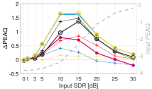
(b) SMALL: Music ($\Delta$PEAQ)

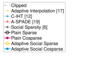
(c) SMALL: Legend

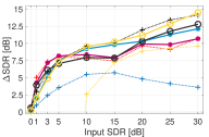
(d) SMALL: Speech ($\Delta$SDR)

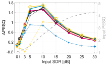
(e) SMALL: Speech ($\Delta$PESQ)

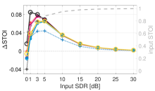
(f) SMALL: Speech ($\Delta$STOI)

Figure 8: State-of-the-art comparison (Signal-based & perceptually-motivated objective quality measures) on SMALL dataset.

Table IV: State-of-the-art comparison on SMALL dataset (Mean $\pm$ std) of $\Delta$SDR

Input SDR [dB]	Adaptive Interpolation [17]	C-IHT [12]	A-SPADE [19]	Social Sparsity [6]	Plain Sparse	Plain Cosparse	Adaptive Social Sparse	Adaptive Social Cosparse
0	-1.4$\pm$2.5	0.1$\pm$0.03	0.001$\pm$0.003	0.3$\pm$0.1	0.7$\pm$0.1	0.5$\pm$0.07	0.2$\pm$0.1	0.2$\pm$0.05
1	-6.8$\pm$11.8	1.1$\pm$0.4	5.5$\pm$1.1	3.9$\pm$1.1	5.3$\pm$1.7	4.2$\pm$0.9	1.8$\pm$0.5	1.8$\pm$0.6
3	-3.0$\pm$2	3.1$\pm$1.2	8.3$\pm$2.3	6.9$\pm$2.5	6.4$\pm$1.6	8.1$\pm$1.8	4.8$\pm$1.9	4.8$\pm$2
5	-1.9$\pm$3.9	4.7$\pm$1.6	8.5$\pm$3.2	8.4$\pm$3.1	7.5$\pm$2.3	8.8$\pm$2.7	6.6$\pm$2.7	6.7$\pm$2.7
10	1.5$\pm$8.1	6.7$\pm$2.3	9.3$\pm$4.2	9.8$\pm$5.1	9.0$\pm$3.8	9.9$\pm$3.7	9.2$\pm$4.2	8.9$\pm$4
15	5.8$\pm$6.2	7.0$\pm$2.6	8.6$\pm$5.1	10.1$\pm$5.1	9.0$\pm$4.6	9.9$\pm$4.6	9.7$\pm$5.1	8.9$\pm$4.4
20	6.1$\pm$6.5	6.4$\pm$2.6	7.4$\pm$5.6	9.6$\pm$5	8.0$\pm$5.3	8.8$\pm$4.8	9.4$\pm$5.4	8.8$\pm$4.7
25	6.4$\pm$6.7	6.0$\pm$2.5	6.8$\pm$5.6	9.5$\pm$5.6	8.2$\pm$5.6	8.4$\pm$5	9.4$\pm$5.5	9.0$\pm$4.8
30	5.5$\pm$6.5	5.3$\pm$3.3	5.6$\pm$6.2	8.2$\pm$5.5	7.6$\pm$5.6	7.6$\pm$5.4	8.5$\pm$5.8	7.6$\pm$4.8

(a) SMALL Music

Input SDR [dB]	Adaptive Interpolation [17]	C-IHT [12]	A-SPADE [19]	Social Sparsity [6]	Plain Sparse	Plain Cosparse	Adaptive Social Sparse	Adaptive Social Cosparse
0	-241.4$\pm$6.8	0.1$\pm$0.01	0.0$\pm$0	0.2$\pm$0.05	0.6$\pm$0.08	0.6$\pm$0.02	0.2$\pm$0.04	0.2$\pm$0.03
1	-253.9$\pm$11.3	0.9$\pm$0.2	5.0$\pm$0.8	3.8$\pm$0.7	3.9$\pm$0.5	4.2$\pm$0.3	2.0$\pm$0.4	2.0$\pm$0.4
3	-198.3$\pm$105.9	2.4$\pm$0.4	7.3$\pm$1.5	6.9$\pm$1.1	6.1$\pm$0.6	7.2$\pm$1.1	4.9$\pm$0.9	5.2$\pm$1.1
5	-46.6$\pm$98.1	3.5$\pm$0.5	8.0$\pm$2.1	7.8$\pm$1.8	7.1$\pm$2.3	8.2$\pm$1.7	7.3$\pm$2	7.5$\pm$2
10	2.5$\pm$3.1	5.4$\pm$0.9	7.8$\pm$4.2	9.6$\pm$2.2	8.0$\pm$3.7	8.4$\pm$3.6	9.5$\pm$2.4	9.2$\pm$2.2
15	7.1$\pm$4.8	5.7$\pm$1.1	7.4$\pm$5.3	10.2$\pm$3.3	7.9$\pm$4.9	7.9$\pm$4.9	10.2$\pm$3.3	9.8$\pm$2.7
20	8.8$\pm$5	4.8$\pm$2.3	9.6$\pm$5.4	12.2$\pm$5.4	10.3$\pm$6.5	9.9$\pm$5.5	11.2$\pm$6.5	10.3$\pm$4.7
25	9.3$\pm$6.3	4.1$\pm$3.5	9.1$\pm$7.1	13.3$\pm$6.1	11.8$\pm$8.3	9.8$\pm$7.1	12.9$\pm$6.8	11.3$\pm$5.1
30	9.6$\pm$6.5	3.6$\pm$2.2	10.7$\pm$6.4	14.4$\pm$7.9	12.8$\pm$8.1	10.7$\pm$6	14.5$\pm$8.2	12.1$\pm$5.3

(b) SMALL Speech

State-of-the-art comparisons are first conducted on the 20 audio examples from the SMALL dataset described in the introduction, for its wide use in the literature, and as a preliminary tuning for subsequent experiments.

Then, the proposed large scale objective experiments are conducted on excerpts from the RWC Music Database [38]. We use the “Pop” and “Jazz” genres as is, and subcategorize the “Classic” genre (Vocals, Chamber, Symphonies), leading to 5 subsets. All the tracks are sufficiently diverse to reflect the robustness of the approach on different audio content. We also perform experiments on excerpts of the TIMIT database [39] for evaluation on speech content.

All the audio examples used for objective experiments are either natively sampled at 16 kHz or down-sampled to 16 kHz, and down-mixed (by simple averaging of the two channels) to provide single-channel data. Each excerpt was normalized in amplitude ($\|\text{vec}(\boldsymbol{\mathbf{{X}}})\|_{\infty}=1$) then artificially clipped under the hard-clipping model in (1) to meet a given input SDR. Table III summarizes the data used for these experiments.

Remark.

Since existing small scale benchmarks were conducted at 16 kHz, and given the substantial increase in computational resources that would be needed to conduct benchmarks on 44.1 kHz audio, we keep the 16 kHz format for the large-scale experiments, putting the focus on the diversity of considered musical genres. A different option is to consider less diverse audio files at 44.1 kHz. This is the complementary approach of the parallel and independent survey [13].

Additionally, we perform listening tests based on the MUltiple Stimuli with Hidden Reference and Anchor (MUSHRA) evaluation procedure [40]. We use the webMUSHRA framework [41] and use saturated versions of some original 44.1 kHz stereo excerpts of the 5 RWC subsets, used also (in a 16 kHz monophonic version) for objective experiments. Further details are given in subsection V-E.

V-B Performance measure

As mentioned before, in this work we use the SDR as an objective quality measure of a (de)clipped audio excerpt. Hence, an audio declipping algorithm can be considered performant if, when applied to a clipped signal with low input SDR, it recovers signal with significantly higher SDR. This is naturally captured by the $\Delta$SDR performance measure.

On top of $\Delta$SDR as a first objective measure, we provide perceptually-motivated objective measures of speech quality based on MOS-PESQ scores [16], and analyze a real-valued index predicting intelligibility through the Short-Time Objective Intelligibility (STOI) [42]. For music, we compute the Objective Difference Grade (ODG) PEAQ scores [43] on the entire collection of RWC excerpts. PEAQ scores are computed on 48 kHz upsampled version of the signals using the open-source implementation available with [15]. Finally, for all methods we compare computation times displaying the ratio to real-time processing ($\times$RT).

V-C Small scale objective experiments

In the following we compare the various instances of the proposed generic algorithmic framework with two baseline declipping methods: Adaptive interpolation [17] and Consistent Iterative Hard-Thresholding (C-IHT, [12]), as well as with state-of-the-art methods: the Social Sparsity Declipper [6] and the Analysis SParse Audio DEclipper (A-SPADE, [19]). The plain cosparse algorithm mainly differs from A-SPADE in terms of the relative norm criterion used to stop the procedure. This new choice provides substantial improvements for light to moderate clipping conditions (see Figure 8a).

Common algorithm parameters are set as listed below.

• Frame size $\mathsf{L}$ is the number of samples corresponding to the frame duration of $64$ ms for music, and $32$ ms for speech;

• Square-root periodic Hamming windows, overlap: $75\leavevmode\nobreak\ \%$, for methods allowing frame-based processing;

• Maximum number of iterations $\mathsf{i}_{\max}=10^{6};$

• Analysis operator, $\boldsymbol{\mathbf{{A}}}=$ twice redundant DFT;

• Synthesis operator, $\boldsymbol{\mathbf{{D}}}=$ twice redundant inverse DFT ($\boldsymbol{\mathbf{{D}}}=\boldsymbol{\mathbf{{A}}}^{\mathsf{H}}$).

As the temporal neighbourhood size is given by ${\mathsf{b}=2\mathsf{T}+1}$, setting $\mathsf{T}=5$ for music and $\mathsf{T}=1$ for speech, yields the observation matrices $\boldsymbol{\mathbf{{Y}}}\in{\mathbb{R}^{\mathsf{\mathsf{L}\times\mathsf{11}}}}$ and $\boldsymbol{\mathbf{{Y}}}\in{\mathbb{R}^{\mathsf{\mathsf{L}\times\mathsf{3}}}}$, respectively.

For each algorithm, we choose the stopping criterion $\beta\in\{10^{-1},10^{-2},10^{-3},10^{-4}\}$ that provides the best averaged SDR improvement. The value $\beta=10^{-3}$ appeared as a good comon choice to allow all algorithms to be simulteanously close to their optimal performance. This value will be re-used for all algorithms in the large-scale experiments described in the next section.

Table V: Computational performance of declipping methods (Ratio to real-time processing $\times$RT)

Input SDR [dB]	Adaptive Interpolation [17]	C-IHT [12]	A-SPADE [19]	Social Sparsity [6] LTFAT	Social Sparsity [6] Compiled LTFAT	Plain Sparse	Plain Cosparse	Adaptive Social Sparse	Adaptive Social Cosparse
0	134.6	19.4	0.07	754.2	62.1	5.2	10.1	303.7	296.7
1	82.2	19	17.7	753.3	62.2	6.9	11	236.7	205.7
3	47	17.2	24.9	754.8	62.2	8.7	12.8	191.1	165.4
5	30.5	14.9	27.3	754.5	62.1	9.5	13.5	302.9	143.8
10	12.9	9.8	24.4	755.4	62.1	10.1	13.3	169.6	121
15	6.5	5.7	16.5	754.6	62.1	9.3	11.4	163.5	180.5
20	3.8	3.4	10.4	756.1	62.2	7.6	9.1	70.2	91.7
25	2.2	2.2	6.6	754.6	62.1	2.2	6.2	56	47.4
30	1.3	1.3	4.2	756.4	62.2	3.4	4.1	25.3	22.4

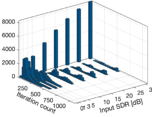
(a) Plain sparse

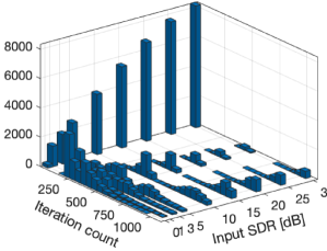
(b) Plain Cosparse

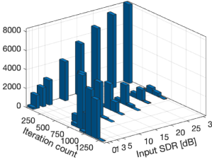
(c) Adaptive social sparse

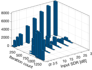
(d) Adaptive social cosparse

Figure 9: Total iteration count distribution on SMALL dataset.

The pattern $\Gamma$ for the non-adaptive social sparse method is fixed as recommended in [6] to obtain the best results. Namely, the patterns extend only in the temporal dimension ($\Gamma\in{\mathbb{R}^{\mathsf{\mathsf{1}\times\mathsf{(2T+1)}}}}$), where $\mathsf{T}=1$ for speech, and $\mathsf{T}=3$ for music signals. Considering the adaptive social (co)sparse declippers, we set the collection of time-frequency patterns $\left\{\Gamma_{\mathsf{k}}\right\}_{\mathsf{k}=1}^{\mathsf{K}}$ to match the one presented on Figure 6 for music and Figure 7 for speech.

For each pattern, the initial shrinkage strength in Algorithm 2 is set as $\mu_{\mathsf{k}}^{\mathsf{(0)}}:=\|\Gamma_{\mathsf{k}}\|_{0}\times\left(1-\|\text{vec}(\boldsymbol{\mathbf{{Y}}})\|_{\infty}\right)$. With this choice, the more severely clipped is the signal $\boldsymbol{\mathbf{{Y}}}$, the lower its magnitude $\|\text{vec}(\boldsymbol{\mathbf{{Y}}})\|_{\infty}$, hence the stronger the shrinkage. Moreover, given the expression (6) of PEW shrinkage, setting $\mu$ proportional to the sparsity degree $\|\Gamma\|_{0}$ of the considered time-frequency neighborhood makes it act as a threshold on the average time-frequency power in this neighborhood, rather than a threshold on the total energy in $\Gamma$.

Once the proper $\Gamma_{\mathsf{k}^{\star}}$ is selected, we obtained the best declipping results with $\mu$ following a geometric progression of common ratio $\alpha$ with $\alpha=0.99$.

Figure 8 displays average SDR improvements, predicted quality improvements ($\Delta$PEAQ, $\Delta$PESQ) and intelligibility improvements ($\Delta$STOI) for all the aforementioned methods on the SMALL examples. To supplement the graphical representation, the average and standard deviation of the $\Delta$SDR measure are given in Table IV . Based on these results, we note that for severe clipping thresholds (low input SDR), plain (co)sparse models provide better SDR improvements than social sparse models. In contrast, we notice superiority of methods that include social sparse models for lighter degradation (input SDR $\geq 15$ dB) and for perceptually-motivated objective quality measure improvements ($\Delta$PEAQ).

Table V presents computational efficiency corresponding to the results obtained in Figure 8. All the experiments were performed using a $\text{Matlab}^{\circledR}\leavevmode\nobreak\$implementation of the algorithms on a workstation equipped with a 2.4 GHz $\text{Intel}^{\circledR}\leavevmode\nobreak\ \text{Xeon}^{\circledR}$processor and 32 GB of RAM. We note that the method provided in [6] uses the Structured Sparsity Toolbox relying on the Large Time-Frequency Analysis Toolbox [44]. We note that for almost all methods, at input SDR of 5 dB or more, the processing time seems to be monotonically decreasing with the input SDR. The exception is for [6] whose computational efficiency seems to be independent from the input SDR. The plausible explanation is that contrary to the other methods, it only relies on an upper bound on the iteration count to stop the algorithm. Hence, the corresponding higher computational time could certainly be drastically reduced by lowering the maximum iteration count.

Remark.

Tuning the parametrization of the plain (co)sparse methods (in particular increasing $\beta$, reducing the number of iterations or increasing the rate of decay of the shrinkage strength) makes it possible to achieve real-time processing on a regular laptop computer, possibly at the cost of tradeoffs with the resulting declipping performance. We also note that for [6] some code optimization (i.e., C backend for the LTFAT toolbox) can drastically improve the computational performance (see. the $\text{4}^{\text{th}}$column of Table V). For the four methods presented here, the maximum number of iteration $\mathsf{i}_{\max}=10^{6}$ is never reached anyway as shown in Figure 9 for a given $\beta=10^{-3}$.

V-D Large scale objective experiments

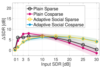
(a) RWC: Pop

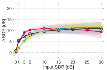
(b) RWC: Jazz

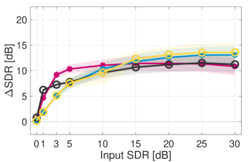
(c) RWC: Orchestra

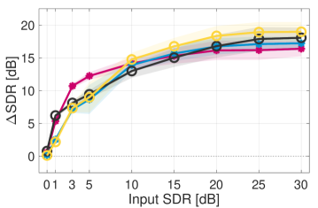
(d) RWC: Vocals

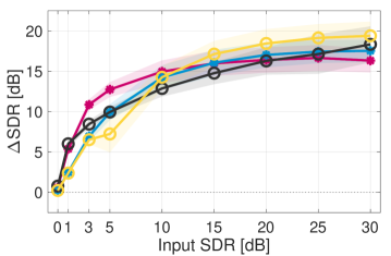
(e) RWC: Chamber

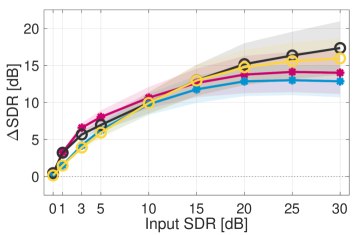
(f) TIMIT: Speech

Figure 10: Performance on large-scale dataset: $\Delta$SDR [dB]

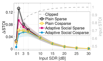
(a) TIMIT: $\Delta$STOI

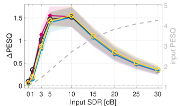
(b) TIMIT: $\Delta$PESQ

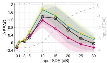
(c) RWC: $\Delta$PEAQ

Figure 11: Performance on large-scale dataset: $\Delta$STOI, $\Delta$PESQ, $\Delta$PEAQ

In order to accurately study the influence of the (social) (co)sparse models, we extend here the study to a wide-range comparison on RWC database excerpts. To the best of our knowledge, it is the first time such a large scale validation is performed. Results presented in Figure 10 and Figure 11 show averaged measurements over all available sounds. In order to assess the effect of different signal models only, we choose a single stopping criterion $\beta$. In light of the experiments on the SMALL dataset, we retained $\beta=10^{-3}$ as a good compromise for the performance of all considered algorithms. Figure 10 shows the behavior of the four methods as a function of the input degradation level. For all the considered datasets, all declipping methods provide significant SDR improvements (often more than $8$ dB) at (almost) all considered input SDRs. This remains the case even for relatively high input SDRs, with one exception: the Pop category, for which the Plain Cosparse brings some degradation at very high input SDR, and the overall improvement never exceeds $8$ dB. This may be due to the fact that most of the 100 unclipped excerpts in this category are mixes containing one or more tracks of dynamically compressed drums, and that at least 21 of them contain saturated guitar sounds. Such sound tracks are intrinsically saturated (on purpose) and it is worth emphasizing that, while the objective of the discussed declipping algorithms is to restore a clipped mix, it is not to restore, e.g., unsaturated guitar sound tracks. This being said, saturating a sound track tends to enrich its spectral content, so that the corresponding mix fails to satisfy the main regularization hypothesis—sparsity in the time-frequency plane—allowing the algorithms to work well.

The benefit of social (co)sparse modeling in terms of these objective measures is clear for high to moderate input SDR ($>10\leavevmode\nobreak\ \text{dB}$, mild clipping), and vice-versa, there is also a distinct superiority of the plain cosparse method for low input SDRs (strong clipping). These tendency will also be observed in listening tests at a 3 dB input SDR. Actually, the plain approaches perform 2 to 4 dB better than the adaptive social methods for input SDRs ranging from 1 to 5 dB on audio content from the RWC database. On the opposite, the trend tends to reverse above 10 dB input SDR as the social methods features improvements between 1 and 4 dB (even 7 dB for the Pop category) above the plain (co)sparse techniques. For speech content, the difference is less obvious yet Figure 10f, Figure 11a and Figure 11b displays better improvements either in terms of SDR, STOI or PESQ for the plain sparse declipper.

Standard deviation results (showed on shaded colors) indicate that the social cosparse declipper produces less variable results across examples: we tested 54 configurations of sound categories and input SDRs, and this declipper produced the smallest standard deviation in 67 % of these configurations. We also observed that, for any of the considered algorithms, the variability of the improvement seems to be higher for higher SDR.

The difference in performance between the plain and social cosparse declippers on music at low input SDR might come from the nature of the degradation. Indeed, contrary to additive noise, clipping adds broadband stripes in the time-frequency plane due to discontinuities of the derivative in the time domain. This way, the signal’s underlying structure (embodied by a time-frequency pattern $\Gamma$) is not only hidden as it would be in the case of additive noise, but also possibly distorted: during the initialization loop of the adaptive social approaches, it is possible that a “wrong” pattern $\Gamma^{*}$ is selected. In contrast, the plain cosparse declipper cannot be affected by this type of behaviour. Another interesting result which could support this hypothesis is that for higher SDR, the social methods are actually benefiting from the time-frequency structure identification as the adaptive approach performs better.

To ease the comparison of the listening tests that come next (conducted on 44.1 kHz audio material) with the PEAQ results of Figure 11 (conducted on 16 kHz material), we conduct additional experiments: for each channel of each 44.1 kHz stereo sample used in the listening test, we computed an objective performance using PEAQ, both on: a) the original 44.1 kHz channel and its clipped+declipped counterpart 44.1 kHz channel; and b) a 16 kHz version of the channel and its clipped+declipped (all at 16 kHz) counterpart. The average results show differences on the order of $0.01$ to $0.1$ on input values of PEAQ and $\Delta$PEAQ.

V-E Listening tests

This listening test is designed using the ITU-R BS.1534-3 recommendation MUSHRA method [40], to provide insights on global audio quality of several declipping methods. To avoid possible difficulties in rating speech quality with non-native speakers participants and as speech intelligibility listening tests are out of the scope of this study, we focus on music excerpts. We evaluate a subset of the conditions presented for the numerical experiments. For the test not to last longer than 30 minutes, we choose a single input SDR of 3 dB. For the sound material, for each genre of the RWC database described in subsection V-A, 2 excerpts of 5 seconds each were randomly picked. The same excerpts were presented to all participants.

We use here the original stereo excerpts sampled at 44.1 kHz to preserve original quality. Each channel is first artificially saturated to reach an identical input SDR level on each channel. Two independant listening tests are performed featuring different initial degradation conditions: $3$ dB and $10$ dB of input SDR.

Each channel of the tested items is processed independently with the 6 best performing sparsity-based methods of Figure 8a and two anchors. The compared methods are here A-SPADE [19], Social sparsity declipper [6], and the 4 variants of the framework presented earlier: plain cosparse, plain sparse, adaptive social cosparse, adaptive social sparse. As a lower anchor, we use the algorithm of [17] based on auto-regressive modeling and interpolation. As Figure 9 suggests that the four algorithms presented here stop far below $10^{6}$ iterations, we set here $\mathsf{i}_{\text{max}}=1300$, the other parameters match those used described earlier. Participants are asked to rate the similarity between the clean reference and the processed signals on a scale from 0 to 100. They remotely access the test through a web-browser based interface thanks to the web-MUSHRA framework [41]. 26 participants aged between 18 and 48 years old volunteered for this listening study. 3 of them reported themselves as expert listeners for audio quality ratings. 23 volunteered for the $3$ dB input SDR condition and 14 volunteered for the $10$ dB input SDR testing condition. Figure 12 displays results for this listening experiment.

For the $3$ dB input SDR condition, despite the variability between participants, a repeated measures analysis of variance (ANOVA) and t-paired tests [45] reveal that the average results for the lower anchor [17] and the plain sparse algorithm are significantly different from (and lower than) the 5 other methods (p-values $\leq 9\cdot 10^{-8}$). Even if these results do not show statistically significant different means between A-SPADE [19], the Social sparsity declipper [6], adaptive social (co)sparse and plain cosparse algorithms, individual results shows the same ranking trend from one participant to another.

For the second testing condition ($10$ dB input SDR), results show very similar ratings between all sparsity-based methods and the reference. Only the lower anchor [17] shows significant differences with the other methods (p-values $\leq 8\cdot 10^{-8}$). Results for this lighter input degradation condition also show comparable median results between the reference and methods using adaptive-social and/or analysis sparse models. This suggests that it might be difficult to discriminate between the restored and reference signals for such input degradation model. Hence, further SDR improvements in this type of testing condition might not be so important when targeting perceived audio quality.

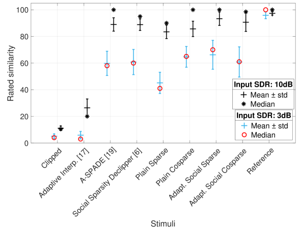
Figure 12: Audio rating via listening tests

VI Conclusion

Recent progress in audio declipping has made it possible to address severe degradation levels with unprecedented performance. The versatile algorithmic framework proposed here, which handles transparently both the analysis and synthesis variants of sparse time-frequency models as well as the popular “social” time-frequency constraint, allowed us to conduct a systematic evaluation of many popular algorithms, in addition to a novel variant (adaptive social cosparse). The systematic coverage of algorithmic options and of a large ballpark of clipping thresholds, evaluated on a wide range of data and performance measures, lead us to draw conclusions and guidelines for the practice of declipping as well as its performance evaluation.

The first message to be drawn is the importance of experimental methodology to truly assess declipping performance, which should consider: i) measuring the initial degradation and its improvement in terms of Signal-to-Distortion Ratio; ii) choosing a perceptually relevant range of degradation levels, more ambitious than the one used in early work on the topic, down to only a few decibels; iii) as in many other fields (if not all), gathering large test sets, covering a wide scope of musical genres and speech; iv) conducting listening tests.

In terms of algorithmic choices, we can summarize our observations as follows. The first expected result is the supremacy of sparsity-based methods (no matter the variant) over the well-established autoregressive interpolation method, in all clipping regimes but the inaudible ones. For light clipping regimes (Input SDR above 5 dB), recent sparse methods consistently bring improvements of 8 dB and more for various types of speech and music. Significant improvements, typically of a few decibels and up to 10 dB, are also obtained by these methods in severe clipping cases (input SDR from 0 to 5 dB). The only notable exception is pop music, possibly due to the presence of dynamically compressed drums and saturated guitar sounds. Similar trends are observed with perceptually-motivated objective quality measures.

The plain and social variants have comparable quantitative restoration performance, although the social constraint brings more benefit at mild clipping regimes; plain versions could be preferable in more challenging conditions. This could be due to the difficulty to detect social sparsity patterns heavily corrupted by strong clipping, and calls for further studies to guide the choice of such patterns, possibly based on learning techniques. However, from a perceptual point of view, adaptive social algorithms were slightly preferred by listeners, even at 3 dB.

Improvements brought by the social constraint, however, comes with an increased computational cost. While cosparsity has been previously thought to be faster in the declipping task [19], better implementations and a fair tuning of stopping criteria suggest here that synthesis models are still on the go. Finally, at the moment, only plain versions show an immediate potential for real-time applications.

The algorithmic framework for audio restoration proposed in this paper is versatile from many points of view. In particular, it can handle several types of audio distortion models: demonstrated here on declipping, it can act as well on denoising and dereverberation problems [46]. Further work could include extensions of the framework to these degradations, and multichannel scenarios.

[Generalized projection for declipping]

For the synthesis case, solving (7) with $\Theta=\Theta_{\textrm{time-freq}}(\boldsymbol{\mathbf{{Y}}})$ and $\boldsymbol{\mathbf{{M}}}=\boldsymbol{\mathbf{{I}}}$ can be recast as:

$$\hat{\boldsymbol{\mathbf{{W}}}}=\operatorname*{argmin}_{\boldsymbol{\mathbf{{W}}}}\|\boldsymbol{\mathbf{{W}}}-\boldsymbol{\mathbf{{Z}}}\|_{\text{F}}^{2}\operatorname*{\,subject\,to\,}\boldsymbol{\mathbf{{D}}}\boldsymbol{\mathbf{{W}}}\in\tilde{\Theta}$$ (11)

and

$$\tilde{\Theta}:=\left\{\boldsymbol{\mathbf{{V}}}\ |\begin{array}[]{l}\boldsymbol{\mathbf{{V}}}_{\Omega_{r}}=\boldsymbol{\mathbf{{Y}}}_{\Omega_{r}};\\ \boldsymbol{\mathbf{{V}}}_{\Omega_{+}}\succcurlyeq\boldsymbol{\mathbf{{Y}}}_{\Omega_{+}};\\ \boldsymbol{\mathbf{{V}}}_{\Omega_{-}}\preccurlyeq\boldsymbol{\mathbf{{Y}}}_{\Omega_{-}}.\end{array}\right\}.$$

As shown in [31, 47], when $\boldsymbol{\mathbf{{D}}}\boldsymbol{\mathbf{{D}}}^{\mathsf{H}}=\boldsymbol{\mathbf{{I}}}$ and $\tilde{\Theta}$ embodies a multidimensional interval constraint, the closed-form solution for (11) writes:

$$\hat{\boldsymbol{\mathbf{{W}}}}=\boldsymbol{\mathbf{{Z}}}-\boldsymbol{\mathbf{{D}}}^{\mathsf{H}}(\boldsymbol{\mathbf{{D}}}\boldsymbol{\mathbf{{Z}}}-\Pi(\boldsymbol{\mathbf{{Z}}})),$$ (12)

with

$$[\Pi(\boldsymbol{\mathbf{{Z}}})]_{\mathsf{nt}}\leavevmode\nobreak\ =\leavevmode\nobreak\ \left\{\begin{array}[]{l l}(\boldsymbol{\mathbf{{D}}}\boldsymbol{\mathbf{{Z}}})_{\mathsf{nt}}&\text{if\leavevmode\nobreak\ }\left\{\begin{array}[]{l}\mathsf{nt}\in\Omega_{+},(\boldsymbol{\mathbf{{D}}}\boldsymbol{\mathbf{{Z}}})_{\mathsf{nt}}\geq\tau;\\ \text{or}\\ \mathsf{nt}\in\Omega_{-},(\boldsymbol{\mathbf{{D}}}\boldsymbol{\mathbf{{Z}}})_{\mathsf{nt}}\leq-\tau;\end{array}\right.\\ \boldsymbol{\mathbf{{Y}}}_{\mathsf{nt}}&\text{otherwise.}\\ \end{array}\right.$$

References

- [1] C.-T. Tan, B. C. Moore, and N. Zacharov, “The effect of nonlinear distortion on the perceived quality of music and speech signals,” Journal of the Audio Engineering Society, vol. 51, no. 11, pp. 1012–1031, 2003.
- [2] Y. Tachioka, T. Narita, and J. Ishii, “Speech recognition performance estimation for clipped speech based on objective measures,” Acoustical Science and Technology, vol. 35, no. 6, pp. 324–326, 2014.
- [3] M. J. Harvilla and R. M. Stern, “Least squares signal declipping for robust speech recognition,” in Fifteenth Annual Conference of the International Speech Communication Association, 2014.
- [4] C. Laguna and A. Lerch, “An efficient algorithm for clipping detection and declipping audio,” in Audio Engineering Society Convention 141. Audio Engineering Society, 2016.
- [5] A. Adler, V. Emiya, M. G. Jafari, M. Elad, R. Gribonval, and M. D. Plumbley, “Audio inpainting,” IEEE Transactions on Audio, Speech, and Language Processing, vol. 20, no. 3, pp. 922–932, 2012.
- [6] K. Siedenburg, M. Kowalski, and M. Dörfler, “Audio declipping with social sparsity,” in 2014 IEEE International Conference on Acoustics, Speech and Signal Processing (ICASSP), 2014, pp. 1577–1581.
- [7] A. Ozerov, Ç. Bilen, and P. Pérez, “Multichannel audio declipping,” in 2016 IEEE International Conference on Acoustics, Speech and Signal Processing (ICASSP), 2016, pp. 659–663.
- [8] I. Damnjanovic, M. E. Davies, and M. D. Plumbley, “Smallbox - an evaluation framework for sparse representations and dictionary learning algorithms,” in International Conference on Latent Variable Analysis and Signal Separation (LVA/ICA). Springer, 2010, pp. 418–425.
- [9] L. Rencker, F. Bach, W. Wang, and M. D. Plumbley, “Consistent dictionary learning for signal declipping,” in International Conference on Latent Variable Analysis and Signal Separation (LVA/ICA). Springer, 2018, pp. 446–455.
- [10] P. Záviška, P. Rajmic, O. Mokrý, and Z. Průša, “A proper version of synthesis-based sparse audio declipper,” in 2019 IEEE International Conference on Acoustics, Speech and Signal Processing (ICASSP), 2019, pp. 591–595.
- [11] E. Vincent, S. Araki, F. J. Theis, G. Nolte, P. Bofill, H. Sawada, A. Ozerov, B. V. Gowreesunker, D. Lutter, and N. Q. K. Duong, “The Signal Separation Evaluation Campaign (2007-2010): Achievements and Remaining Challenges,” Inria, Research Report RR-7581, Mar. 2011. [Online]. Available: https://hal.inria.fr/inria-00579398
- [12] S. Kitic, L. Jacques, N. Madhu, M. P. Hopwood, A. Spriet, and C. De Vleeschouwer, “Consistent iterative hard thresholding for signal declipping,” in 2013 IEEE International Conference on Acoustics, Speech and Signal Processing (ICASSP), 2013, pp. 5939–5943.
- [13] P. Záviska, P. Rajmic, A. Ozerov, and L. Rencker, “A survey and an extensive evaluation of popular audio declipping methods,” Jul. 2020. [Online]. Available: https://arxiv.org/abs/2007.07663v1
- [14] B. Defraene, N. Mansour, S. De Hertogh, T. van Waterschoot, M. Diehl, and M. Moonen, “Declipping of audio signals using perceptual compressed sensing,” IEEE Transactions on Audio, Speech, and Language Processing, vol. 21, no. 12, pp. 2627–2637, 2013.
- [15] P. Kabal, “An examination and interpretation of itu-r bs. 1387: Perceptual evaluation of audio quality,” TSP Lab Technical Report, Dept. Electrical & Computer Engineering, McGill University, pp. 1–89, 2002.
- [16] A. W. Rix, J. G. Beerends, M. P. Hollier, and A. P. Hekstra, “Perceptual evaluation of speech quality (pesq)-a new method for speech quality assessment of telephone networks and codecs,” in 2001 IEEE International Conference on Acoustics, Speech, and Signal Processing (ICASSP), vol. 2, 2001, pp. 749–752 vol.2.
- [17] A. J. E. M. Janssen, R. N. J. Veldhuis, and L. Vries, “Adaptive interpolation of discrete-time signals that can be modeled as autoregressive processes,” IEEE Transactions on Acoustics, Speech and Signal Processing, vol. 34, no. 2, pp. 317–330, 1986.
- [18] F. R. Ávila, M. P. Tcheou, and L. W. Biscainho, “Audio soft declipping based on constrained weighted least squares,” IEEE Signal Processing Letters, vol. 24, no. 9, pp. 1348–1352, 2017.
- [19] S. Kitić, N. Bertin, and R. Gribonval, “Sparsity and cosparsity for audio declipping: a flexible non-convex approach,” in International Conference on Latent Variable Analysis and Signal Separation (LVA/ICA). Springer, 2015, pp. 243–250.
- [20] M. Kowalski, K. Siedenburg, and M. Dörfler, “Social sparsity! neighborhood systems enrich structured shrinkage operators,” IEEE Transactions on Signal Processing, vol. 61, no. 10, pp. 2498–2511, 2013.
- [21] S. Nam, M. E. Davies, M. Elad, and R. Gribonval, “Cosparse analysis modeling - uniqueness and algorithms,” in 2011 IEEE International Conference on Acoustics, Speech and Signal Processing (ICASSP), 2011, pp. 5804–5807.
- [22] S. Kitić, “Cosparse regularization of physics-driven inverse problems,” PhD Thesis, IRISA, Inria Rennes, 2015. [Online]. Available: https://hal.archives-ouvertes.fr/tel-01237323
- [23] M. Kowalski and B. Torrésani, “Structured sparsity: from mixed norms to structured shrinkage,” in SPARS’09-Signal Processing with Adaptive Sparse Structured Representations, 2009.
- [24] R. Jenatton, J.-Y. Audibert, and F. Bach, “Structured variable selection with sparsity-inducing norms,” The Journal of Machine Learning Research, vol. 12, pp. 2777–2824, 2011.
- [25] M. Kowalski and B. Torrésani, “Sparsity and persistence: mixed norms provide simple signal models with dependent coefficients,” Signal, image and video processing, vol. 3, no. 3, pp. 251–264, 2009.
- [26] M. Kowalski, “Sparse regression using mixed norms,” Applied and Computational Harmonic Analysis, vol. 27, no. 3, p. 303–324, 2009.
- [27] M. Kowalski, “Thresholding rules and iterative shrinkage/thresholding algorithm: A convergence study,” in 2014 IEEE International Conference on Image Processing (ICIP), 2014, pp. 4151–4155.
- [28] T. Blumensath and M. E. Davies, “Iterative hard thresholding for compressed sensing,” Applied and Computational Harmonic Analysis, vol. 27, no. 3, pp. 265–274, 2009.
- [29] K. Siedenburg, “Persistent empirical wiener estimation with adaptive threshold selection for audio denoising,” in Proceedings of the 9th Sound and Music Computing Conference, Copenhagen, DK, 2012.
- [30] K. Siedenburg and M. Dörfler, “Audio denoising by generalized time-frequency thresholding,” in 45th Audio Engineering Society Conference: Applications of Time-Frequency Processing in Audio. Audio Engineering Society, 2012.
- [31] P. Rajmic, P. Záviska, V. Veselý, and O. Mokrý, “A New Generalized Projection and Its Application to Acceleration of Audio Declipping.” Axioms, vol. 8, no. 3, p. 105, 2019. [Online]. Available: https://www.mdpi.com/2075-1680/8/3/105
- [32] S. Boyd, N. Parikh, E. Chu, B. Peleato, and J. Eckstein, “Distributed optimization and statistical learning via the alternating direction method of multipliers,” Foundations and Trends® in Machine Learning, vol. 3, no. 1, pp. 1–122, 2011.
- [33] C. Gaultier, S. Kitić, E. Camberlein, R. Gribonval, and N. Bertin, “SPADE Toolbox,” 2019, software. [Online]. Available: https://hal.inria.fr/hal-03024116
- [34] C. Gaultier, S. Kitić, N. Bertin, and R. Gribonval, “Audascity: Audio denoising by adaptive social cosparsity,” in 2017 25th European Signal Processing Conference (EUSIPCO), 2017, pp. 1265–1269.
- [35] H. A. Sturges, “The choice of a class interval,” Journal of the American Statistical Association, vol. 21, no. 153, pp. 65–66, 1926.
- [36] J. O. Smith, Spectral Audio Signal Processing. https://ccrma.stanford.edu/~jos/sasp/Overlap_Add_Decomposition.html, accessed Oct. 3, 2020, ch. Overlap-Add Decomposition, online book, 2011 edition.
- [37] ——, Spectral Audio Signal Processing. https://ccrma.stanford.edu/~jos/sasp/Choice_WOLA_Window.html, accessed Oct. 3, 2020, ch. Choice of WOLA Window, online book, 2011 edition.
- [38] M. Goto, H. Hashiguchi, T. Nishimura, and R. Oka, “RWC music database: Popular, classical and jazz music databases.” in ISMIR, vol. 2, 2002, pp. 287–288.
- [39] J. S. Garofolo, L. F. Lamel, W. M. Fisher, J. G. Fiscus, and D. S. Pallett, “Darpa timit acoustic-phonetic continous speech corpus cd-rom. nist speech disc 1-1.1,” NASA STI/Recon technical report n, vol. 93, 1993.
- [40] “ITU-R BS.1534-1: Method for the subjective assessment of intermediate quality levels of coding systems.”
- [41] M. Schoeffler, S. Bartoschek, F.-R. Stöter, M. Roess, S. Westphal, B. Edler, and J. Herre, “webmushra—a comprehensive framework for web-based listening tests,” Journal of Open Research Software, vol. 6, no. 1, 2018.
- [42] C. H. Taal, R. C. Hendriks, R. Heusdens, and J. Jensen, “An algorithm for intelligibility prediction of time–frequency weighted noisy speech,” IEEE Transactions on Audio, Speech, and Language Processing, vol. 19, no. 7, pp. 2125–2136, 2011.
- [43] T. Thiede, W. C. Treurniet, R. Bitto, C. Schmidmer, T. Sporer, J. G. Beerends, and C. Colomes, “Peaq-the itu standard for objective measurement of perceived audio quality,” Journal of the Audio Engineering Society, vol. 48, no. 1/2, pp. 3–29, 2000.
- [44] P. L. Søndergaard, B. Torrésani, and P. Balazs, “The Linear Time Frequency Analysis Toolbox,” International Journal of Wavelets, Multiresolution Analysis and Information Processing, vol. 10, no. 4, 2012.
- [45] J. Cohen, Statistical power analysis for the behavioral sciences. Academic press, 2013.
- [46] C. Gaultier, “Design and evaluation of sparse models and algorithms for audio inverse problems,” Ph.D. dissertation, 2019.
- [47] M. Šorel and M. Bartoš, “Efficient jpeg decompression by the alternating direction method of multipliers,” in 2016 23rd International Conference on Pattern Recognition (ICPR). IEEE, 2016, pp. 271–276.