Numerical simulations for full history recursive
multilevel Picard approximations for systems of
high-dimensional partial differential equations

Abstract

One of the most challenging issues in applied mathematics is to develop and analyze algorithms which are able to approximately compute solutions of high-dimensional nonlinear partial differential equations (PDEs). In particular, it is very hard to develop approximation algorithms which do not suffer under the curse of dimensionality in the sense that the number of computational operations needed by the algorithm to compute an approximation of accuracy $\varepsilon>0$ grows at most polynomially in both the reciprocal $\nicefrac{{1}}{{\varepsilon}}$ of the required accuracy and the dimension $d\in\mathbb{N}$ of the PDE. Recently, a new approximation method, the so-called full history recursive multilevel Picard (MLP) approximation method, has been introduced and, until today, this approximation scheme is the only approximation method in the scientific literature which has been proven to overcome the curse of dimensionality in the numerical approximation of semilinear PDEs with general time horizons. It is a key contribution of this article to extend the MLP approximation method to systems of semilinear PDEs and to numerically test it on several example PDEs. More specifically, we apply the proposed MLP approximation method in the case of Allen-Cahn PDEs, Sine-Gordon-type PDEs, systems of coupled semilinear heat PDEs, and semilinear Black-Scholes PDEs in up to 1000 dimensions. The presented numerical simulation results suggest in the case of each of these example PDEs that the proposed MLP approximation method produces very accurate results in short runtimes and, in particular, the presented numerical simulation results indicate that the proposed MLP approximation scheme significantly outperforms certain deep learning based approximation methods for high-dimensional semilinear PDEs.

1 Introduction

One of the most challenging issues in applied mathematics is to develop and analyze algorithms which are able to approximately compute solutions of high-dimensional nonlinear partial differential equations (PDEs). In particular, it is very hard to develop approximation algorithms which do not suffer under the curse of dimensionality in the sense that the number of computational operations needed by the algorithm to compute an approximation of accuracy $\varepsilon>0$ grows at most polynomially in both the reciprocal $\nicefrac{{1}}{{\varepsilon}}$ of the required accuracy and the dimension $d\in\mathbb{N}$ of the PDE. In the last four years, very significant progress has been made in this research area, where particularly the following two types of approximation methods have turned out to be very promising:

1. Deep learning based approximation methods for PDEs; cf., e.g., [8, 10, 5, 4, 3, 11, 14, 15, 16, 18, 24, 26, 29, 35, 34, 36, 37, 38, 44, 46, 47, 50, 51, 52, 53, 54, 55, 56, 57, 58, 59, 60, 61, 63, 64, 22, 19, 9]

2. Full history recursive multilevel Picard approximation methods for PDEs; cf., e.g., [20, 43, 41, 39, 21, 7, 27, 42, 6] (in the following we abbreviate full history recursive multilevel Picard by MLP)

Roughly speaking, deep learning based approximation methods for high-dimensional PDEs are often based on the idea

1. to approximate the solution of the considered PDE through the solution of a suitable infinite dimensional stochastic optimization problem on an appropriate function space,

2. to approximate some of the functions appearing in the infinite dimensional stochastic optimization problem by deep neural networks (DNNs) to obtain finite dimensional stochastic optimization problems, and

3. to apply stochastic gradient descent type algorithms to the resulting finite dimensional stochastic optimization problems to approximately learn the optimal parameters of the involved DNNs.

MLP approximation methods have first been proposed in [20, 41] and are, roughly speaking, based on the idea

1. to reformulate the computational problem under consideration as a stochastic fixed point equation on a suitable function space with the fixed point of the fixed point equation being the solution of the computational problem,

2. to approximate the solution of the fixed point equation by means of iterations given by the fixed point equation (which are referred to as Picard iterations in the context of temporal integral fixed point equations), and

3. to approximate the resulting fixed point iterates by suitable multilevel Monte Carlo approximations, which are full history recursive in the sense that for all $n\in\mathbb{N}$ it holds that the multilevel Monte Carlo approximation of the $n$th fixed point iterate is based on evaluations of multilevel Monte Carlo approximations of the $(n-1)$th, $(n-2)$th, …, 2nd, and 1st fixed point iterates.

A key advantage of deep learning based approximation methods for PDEs is that they seem to be applicable to a very wide class of PDEs including semilinear parabolic PDEs (cf, e.g., [3, 34, 19]), elliptic PDEs (cf, e.g., [46, 22]), free boundary PDEs associated to optimal stopping problems (cf, e.g., [8, 10, 9, 29, 15]), and fully nonlinear PDEs (cf, e.g., [5, 58]), while MLP approximation algorithms are limited to the situation where the computational problem can be formulated as a suitable stochastic fixed point equation and thereby (currently) exclude, for example, fully nonlinear PDEs. On the other hand, a key advantage of MLP approximation methods is that, until today, these approximation methods are the only methods for which it has been proven that they overcome the curse of dimensionality in the numerical approximation of semilinear PDEs with general time horizons. In contrast to this, for deep learning based approximation methods there are so far a number of encouraging numerical simulations for PDEs, but only partial error analysis results (see, e.g., [30, 23, 45, 12, 35, 28, 31, 32, 40, 49, 62]) which corroborate the conjecture that deep learning based approximation methods might overcome the curse of dimensionality. These partial error analysis results prove that there exist DNNs which are able to approximate solutions of PDEs with the number of parameters in the DNN growing at most polynomially in both the PDE dimension and the reciprocal of the required approximation accuracy, but there are no results asserting that the employed stochastic optimization algorithm will find such an approximating DNN. Moreover, one should note that in the case of nonlinear PDEs the proofs for the partial error analysis results mentioned above (cf. [40]) are, in turn, strongly based on the fact that MLP approximation schemes overcome the curse of dimensionality (cf. [41]).

The above mentioned articles [20, 43, 41, 39, 7, 27, 42, 6] on MLP approximation algorithms contain proofs that the proposed MLP approximation algorithms overcome the curse of dimensionality for various types of nonlinear PDEs and thereby established, for the first time, that semilinear PDEs can actually be approximated without the curse of dimensionality. However, none of these articles contain numerical simulations. It is the subject of this article to generalize the MLP approximation algorithms in [41, 7, 42] to systems of PDEs and to present numerical simulations for several example PDEs in up to 1000 dimensions. More precisely, in Section 2 we specify the generalized MLP approximation scheme which we propose in this article (see (3) in Section 2 below) and in Section 3 we apply this numerical approximation scheme to four different kinds of semilinear PDEs. We consider Allen-Cahn PDEs in Subsection 3.1, Sine-Gordon type PDEs in Subsection 3.2, systems of coupled semilinear heat PDEs in Subsection 3.3, and semilinear Black-Scholes PDEs in Subsection 3.4. In the case of each of the above mentioned example PDEs we approximately compute the relative $L^{2}$-error of the proposed MLP approximation algorithm (see Table 1 and Figure 1 in Subsection 3.1, Table 2 and Figure 2 in Subsection 3.2, Table 3 and Figure 3 in Subsection 3.3, and Table 4 and Figure 4 in Subsection 3.4). In our approximate computations of the relative $L^{2}$-errors the unknown exact solutions of the PDEs have been approximated by means of the deep learning based approximation method in Beck et al. [3], the so-called deep splitting (DS) method (see the 4 and 5 columns in Tables 1, 2, 3, and 4 and Figures 1(a), 2(a), 3(a), and 4(a)) and by means of the MLP approximation algorithm itself (see the 4 and 6 columns in Tables 1, 2, 3, and 4 and Figures 1(b), 2(b), 3(b), and 4(b)). In Section 4 we present the C++  source code employed to perform the numerical simulations presented in Section 3.

2 Description of the approximation algorithm

In this section we introduce the generalized MLP approximation scheme which we consider in this article (see (3) in Framework 1 below).

Framework 1.

Let $d,k\in\mathbb{N}$, $c,T\in(0,\infty)$, $\Theta=\cup_{n\in\mathbb{N}}\mathbb{Z}^{n}$, $f=(f_{1},\dots,f_{k})\in C(\mathbb{R}^{d}\times\mathbb{R}^{k},\mathbb{R}^{k})$, $g\in C(\mathbb{R}^{d},\mathbb{R}^{k})$, let $\left\|\cdot\right\|\colon(\cup_{q\in\mathbb{N}}\mathbb{R}^{q})\to[0,\infty)$ be the standard norm, let $\phi_{r}\colon\mathbb{R}^{k}\rightarrow\mathbb{R}^{k}$, $r\in[0,\infty]$, satisfy for all $r\in[0,\infty]$, $y=(y_{1},\dots,y_{k})\in\mathbb{R}^{k}$ that

$$\phi_{r}(y)=\left(\min\{r,\max\{-r,y_{1}\}\},\dots,\min\{r,\max\{-r,y_{k}\}\}\right),$$ (1)

let $(\Omega,\mathcal{F},\mathbb{P})$ be a probability space, let $\mathcal{R}^{\theta}\colon\Omega\rightarrow[0,1],$ $\theta\in\Theta$, be independent $\mathcal{U}_{[0,1]}$-distributed random variables, let $W^{\theta}\colon[0,T]\times\Omega\rightarrow\mathbb{R}^{d}$, $\theta\in\Theta$, be independent standard Brownian motions, assume that $(\mathcal{R}^{\theta})_{\theta\in\Theta}$ and $(W^{\theta})_{\theta\in\Theta}$ are independent, let $R^{\theta}\colon[0,T]\times\Omega\rightarrow[0,T]$, $\theta\in\Theta$, satisfy for all $t\in[0,T]$, $\theta\in\Theta$ that $R^{\theta}_{t}=t+(T-t)\mathcal{R}^{\theta}$, let $\mu\colon\mathbb{R}^{d}\to\mathbb{R}^{d}$ and $\sigma\colon\mathbb{R}^{d}\to\mathbb{R}^{d\times d}$ be globally Lipschitz continuous functions, for every $x\in\mathbb{R}^{d}$, $\theta\in\Theta$, $t\in[0,T]$ let $(X^{x,\theta}_{t,s})_{s\in[t,T]}\colon[t,T]\times\Omega\rightarrow\mathbb{R}^{d}$ be a stochastic process with continuous sample paths which satisfies that for all $s\in[t,T]$ it holds $\mathbb{P}$-a.s. that

$$X^{x,\theta}_{t,s}=x+\int_{t}^{s}\mu\big{(}X^{x,\theta}_{t,r}\big{)}\,dr+\int^{s}_{t}\sigma\big{(}X^{x,\theta}_{t,r}\big{)}\,dW^{\theta}_{r},$$ (2)

let $V^{\theta}_{n,M,r}\colon[0,T]\times\mathbb{R}^{d}\times\Omega\rightarrow\mathbb{R}^{k}$, $\theta\in\Theta$, $n\in\mathbb{Z}$, $M\in\mathbb{N}$, $r\in[0,\infty]$, satisfy for all $\theta\in\Theta$, $n,M\in\mathbb{N}$, $r\in[0,\infty]$, $t\in[0,T]$, $x\in\mathbb{R}^{d}$ that $V^{\theta}_{-1,M,r}(t,x)=V^{\theta}_{0,M,r}(t,x)=0$ and

$$\begin{split}V^{\theta}_{n,M,r}(t,x)&=\frac{1}{M^{n}}\Bigg{[}\,\sum_{m=1}^{M^{n}}g\big{(}X^{x,(\theta,0,-m)}_{t,T}\big{)}\Bigg{]}\\ &+\sum_{l=0}^{n-1}\frac{(T-t)}{M^{n-l}}\sum_{m=1}^{M^{n-l}}\bigg{[}f\Big{(}X^{x,(\theta,l,m)}_{t,R_{t}^{(\theta,l,m)}},\phi_{r}\Big{(}V^{(\theta,l,m)}_{l,M,r}\big{(}R_{t}^{(\theta,l,m)},X^{x,(\theta,l,m)}_{t,R_{t}^{(\theta,l,m)}}\big{)}\Big{)}\Big{)}\\ &\qquad-\mathbbm{1}_{\mathbb{N}}(l)\,f\Big{(}X^{x,(\theta,l,m)}_{t,R_{t}^{(\theta,l,m)}},\phi_{r}\Big{(}V^{(\theta,l,-m)}_{l-1,M,r}\big{(}R_{t}^{(\theta,l,m)},X^{x,(\theta,l,m)}_{t,R_{t}^{(\theta,l,m)}}\big{)}\Big{)}\Big{)}\bigg{]},\end{split}$$ (3)

and let $u=(u(t,(x_{1},x_{2},\ldots,x_{d})))_{(t,(x_{1},x_{2},\ldots,x_{d}))\in[0,T]\times\mathbb{R}^{d}}=(u_{1},\dots,u_{k})\in C([0,T]\times\mathbb{R}^{d},\mathbb{R}^{k})$ satisfy for all $t\in[0,T)$, $x\in\mathbb{R}^{d}$, $i\in\{1,2,\dots,k\}$ that $u|_{[0,T)\times\mathbb{R}^{d}}\in C^{1,2}([0,T)\times\mathbb{R}^{d},\mathbb{R}^{k})$, $\left\|u(t,x)\right\|\leq c(1+\left\|x\right\|^{c})$, $u(T,x)=g(x)$, and

$$\begin{split}&(\tfrac{\partial}{\partial t}u_{i})(t,x)+\tfrac{1}{2}\operatorname{Trace}\big{(}\sigma(x)[\sigma(x)]^{*}(\operatorname{Hess}_{x}u_{i})(t,x)\big{)}\\ &+\bigg{[}\textstyle\sum\limits_{j=1}^{d}\mu_{j}(x)(\tfrac{\partial}{\partial x_{j}}u_{i})(t,x)\bigg{]}+f_{i}(x,u(t,x))=0.\end{split}$$ (4)

3 Numerical examples

In this section we apply the MLP approximation algorithm in (3) in Framework 1 above to four different kinds of semilinear PDEs. We consider Allen-Cahn PDEs in Subsection 3.1, Sine-Gordon type PDEs in Subsection 3.2, systems of coupled semilinear heat PDEs in Subsection 3.3, and semilinear Black-Scholes PDEs in Subsection 3.4.

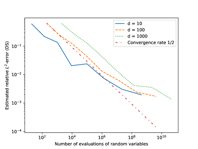
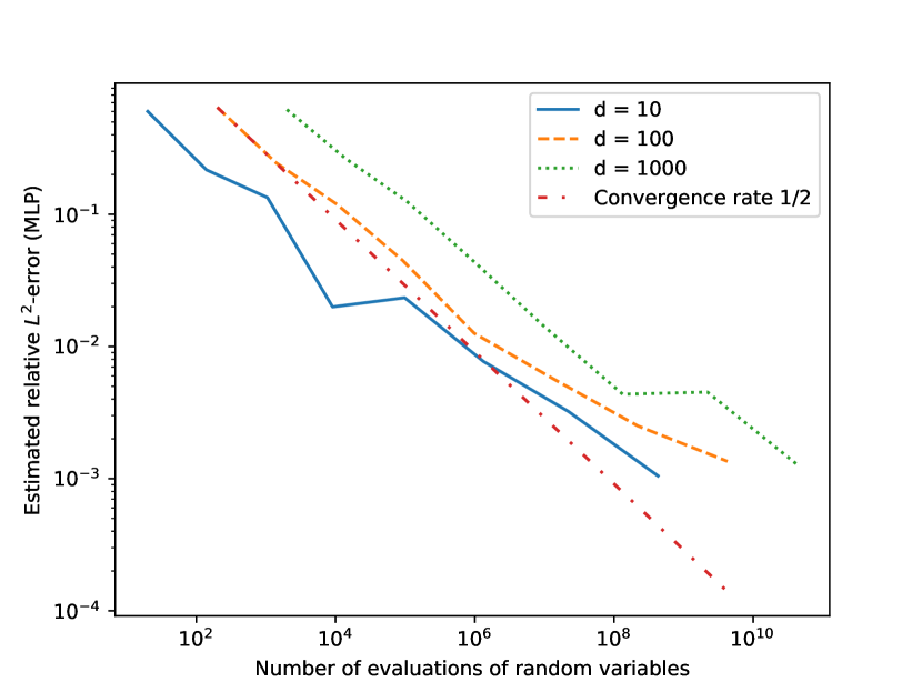
3.1 Allen-Cahn partial differential equations (PDEs)

In this subsection we apply the MLP approximation algorithm in (3) in Framework 1 above to the Allen-Cahn PDE in (5) below (cf., e.g., Bartels [2, Chapter 6] and Feng & Prohl [25]).

Assume Framework 1 and assume for all $t\in[0,T]$, $x,v\in\mathbb{R}^{d}$, $y\in\mathbb{R}$ that $k=1$, $T=1$, $f(x,y)=y-y^{3}$, $g(x)=(2+\tfrac{2}{5}\left\|x\right\|^{2})^{-1}$, $\mu(x)=0$, and $\sigma(x)v=\sqrt{2}v$. Note that this, (2), and (4) assure that for all $x\in\mathbb{R}^{d}$, $\theta\in\Theta$, $t\in[0,T]$, $s\in[t,T]$ it holds that $\mathbb{P}\big{(}X^{x,\theta}_{t,s}=x+\sqrt{2}(W^{\theta}_{s}-W^{\theta}_{t})\big{)}=1$ and

$$(\tfrac{\partial}{\partial t}u)(t,x)+(\Delta_{x}u)(t,x)+u(t,x)-(u(t,x))^{3}=0.$$ (5)

Observe that for all $x\in\mathbb{R}^{d}$, $y\in\mathbb{R}$ it holds that $yf(x,y)=y^{2}-y^{4}\leq 1+y^{2}$. Combining this and (4) with Beck et al. [7, Corollary 2.4] ensures that for all $t\in[0,T]$ it holds that

$$\sup_{x\in\mathbb{R}^{d}}|u(t,x)|\leq e^{T-t}\big{[}1+\sup_{x\in\mathbb{R}^{d}}|u(T,x)|^{2}\big{]}^{\!\nicefrac{{1}}{{2}}}\leq e\big{[}1+\tfrac{1}{4}\big{]}^{\!\nicefrac{{1}}{{2}}}=\frac{\sqrt{5}e}{2}\leq 4.$$ (6)

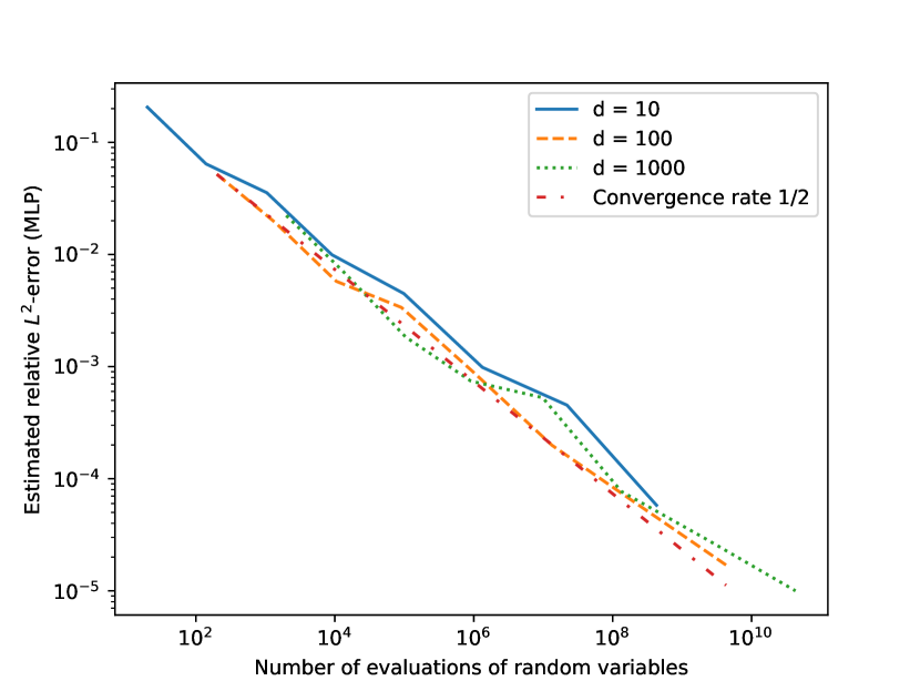
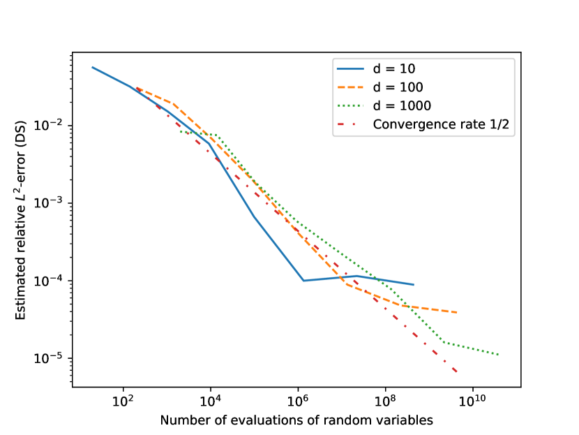
In Table 1 we approximately present for $d\in\{10,100,1000\}$, $n\in\{1,2,\ldots,8\}$ one random realization of $V^{\theta}_{n,n,4}(0,0)$ (3 column in Table 1), the relative $L^{2}$-error $\frac{(\mathbb{E}[|V^{(0)}_{n,n,4}(0,0)-u(0,0)|^{2}])^{1/2}}{u(0,0)}$ (5 and 6 column in Table 1), the number of evaluations of one-dimensional random variables used to calculate one random realization of $V^{\theta}_{n,n,4}(0,0)$ (7 column in Table 1), and the runtime to calculate one random realization of $V^{\theta}_{n,n,4}(0,0)$ (8 column in Table 1). In Figure 1 we approximately plot for $d\in\{10,100,1000\}$, $n\in\{1,2,\ldots,8\}$ the relative $L^{2}$-error $\frac{(\mathbb{E}[|V^{(0)}_{n,n,4}(0,0)-u(0,0)|^{2}])^{1/2}}{u(0,0)}$ (5 and 6 column in Table 1) against the number of evaluations of one-dimensional random variables used to calculate one random realization of $V^{\theta}_{n,n,4}(0,0)$ (7 column in Table 1). The results in Table 1 and Figure 1 have been computed by means of C++ code LABEL:code in Section 4 below. For every $n\in\{1,2,\ldots,8\}$ for our approximative computations of the relative $L^{2}$-error $\frac{(\mathbb{E}[|V^{(0)}_{n,n,4}(0,0)-u(0,0)|^{2}])^{1/2}}{u(0,0)}$ (5 and 6 column in Table 1) the value $u(0,0)$ of the unknown exact solution in the relative $L^{2}$-error has been approximated by means of an average of 5 independent runs of the deep splitting approximation method in Beck et al. [3] (5 column in Table 1) and by means of an average of 5 independent evaluations of $V^{(0)}_{8,8,4}(0,0)$ (6 column in Table 1), respectively, and the expectation in the relative $L^{2}$-error has been approximated by means of Monte Carlo approximations involving 5 independent runs.

d	n	Result of MLP algo- rithm	Refe- rence solu- tions	Esti- mated relative $L^{2}$-error (DS)	Esti- mated relative $L^{2}$-error (MLP)	Evaluations of random variables	Run- time in sec- onds
10	1	0.09925		0.601730	0.600980	20	0.00016
10	2	0.22436	DS:	0.218321	0.216805	140	0.00012
10	3	0.24525	0.29614	0.135595	0.133916	1050	0.00059
10	4	0.28409		0.020630	0.019931	9080	0.00323
10	5	0.30594		0.023919	0.023377	98300	0.03291
10	6	0.29642	MLP:	0.007396	0.007699	1334340	0.45886
10	7	0.29662	0.29555	0.003047	0.003228	22032010	4.16987
10	8	0.29555		0.001953	0.001049	428332080	105.098
100	1	0.01350		0.645486	0.645186	200	0.00006
100	2	0.02433	DS:	0.246201	0.245570	1400	0.00012
100	3	0.03433	0.03376	0.119473	0.118891	10500	0.00087
100	4	0.03345		0.045691	0.045087	90800	0.00857
100	5	0.03332		0.013188	0.012581	983000	0.09031
100	6	0.03346	MLP:	0.006225	0.005701	13343400	1.29344
100	7	0.03375	0.03373	0.002386	0.002504	220320100	25.3006
100	8	0.03373		0.001714	0.001351	4283320800	827.336
1000	1	0.00128		0.620073	0.620698	2000	0.00011
1000	2	0.00253	DS:	0.262782	0.263995	14000	0.00063
1000	3	0.00298	0.00339	0.124379	0.125679	105000	0.00446
1000	4	0.00366		0.045096	0.045392	908000	0.04711
1000	5	0.00338		0.013440	0.014241	9830000	0.56212
1000	6	0.00340	MLP:	0.004158	0.004351	133434000	7.77024
1000	7	0.00340	0.00340	0.003561	0.004518	2203201000	209.154
1000	8	0.00340		0.001379	0.001278	42833208000	7786.58

Table 1: Numerical simulations for the MLP approximation algorithm in (3) in the case of the Allen-Cahn PDE in (5)

(a) Reference solutions computed by DS

(b) Reference solutions computed by MLP

Figure 1: Approximative plot of the relative $L^{2}$-error of the MLP approximation algorithm in (3) against the computational effort of the algorithm in the case of the Allen-Cahn PDE in (5).

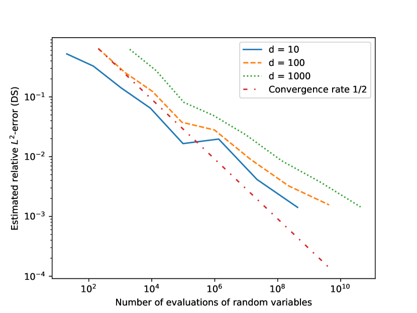
3.2 Sine-Gordon type PDEs

In this subsection we apply the MLP approximation algorithm in (3) in Framework 1 above to the Sine-Gordon-type PDE in (7) below (cf., e.g., Hairer & Hao [33], Barone [1], and Coleman [17]).

Assume Framework 1 and assume for all $t\in[0,T]$, $x,v\in\mathbb{R}^{d}$, $y\in\mathbb{R}$ that $k=1$, $T=1$, $f(x,y)=\sin(y)$, $g(x)=(2+\tfrac{2}{5}\left\|x\right\|^{2})^{-1}$, $\mu(x)=0$, and $\sigma(x)v=\sqrt{2}v$. This, (2), and (4) ensure that for all $x\in\mathbb{R}^{d}$, $\theta\in\Theta$, $t\in[0,T]$, $s\in[t,T]$ it holds that $\mathbb{P}\big{(}X^{x,\theta}_{t,s}=x+\sqrt{2}(W^{\theta}_{s}-W^{\theta}_{t})\big{)}=1$ and

$$(\tfrac{\partial}{\partial t}u)(t,x)+(\Delta_{x}u)(t,x)+\sin(u(t,x))=0.$$ (7)

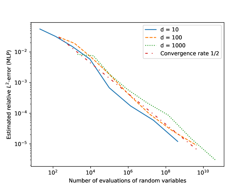
In Table 2 we approximately present for $d\in\{10,100,1000\}$, $n\in\{1,2,\ldots,8\}$ one random realization of $V^{\theta}_{n,n,\infty}(0,0)$ (3 column in Table 2), the relative $L^{2}$-error $\frac{(\mathbb{E}[|V^{(0)}_{n,n,\infty}(0,0)-u(0,0)|^{2}])^{1/2}}{u(0,0)}$ (5 and 6 column in Table 2), the number of evaluations of one-dimensional random variables used to calculate one random realization of $V^{\theta}_{n,n,\infty}(0,0)$ (7 column in Table 2), and the runtime to calculate one random realization of $V^{\theta}_{n,n,\infty}(0,0)$ (8 column in Table 2). In Figure 2 we approximately plot for $d\in\{10,100,1000\}$, $n\in\{1,2,\ldots,8\}$ the relative $L^{2}$-error $\frac{(\mathbb{E}[|V^{(0)}_{n,n,\infty}(0,0)-u(0,0)|^{2}])^{1/2}}{u(0,0)}$ (5 and 6 column in Table 2) against the number of evaluations of one-dimensional random variables used to calculate one random realization of $V^{\theta}_{n,n,\infty}(0,0)$ (7 column in Table 2). The results in Table 2 and Figure 2 have been computed by means of C++ code LABEL:code in Section 4 below. For every $n\in\{1,2,\ldots,8\}$ for our approximative computations of the relative $L^{2}$-error $\frac{(\mathbb{E}[|V^{(0)}_{n,n,\infty}(0,0)-u(0,0)|^{2}])^{1/2}}{u(0,0)}$ (5 and 6 column in Table 2) the value $u(0,0)$ of the unknown exact solution in the relative $L^{2}$-error has been approximated by means of an average of 5 independent runs of the deep splitting approximation method in Beck et al. [3] (5 column in Table 2) and by means of an average of 5 independent evaluations of $V^{(0)}_{8,8,\infty}(0,0)$ (6 column in Table 2), respectively, and the expectation in the relative $L^{2}$-error has been approximated by means of Monte Carlo approximations involving 5 independent runs.

d	n	Result of MLP algo- rithm	Refe- rence solu- tions	Esti- mated relative $L^{2}$-error (DS)	Esti- mated relative $L^{2}$-error (MLP)	Evaluations of random variables	Run- time in sec- onds
10	1	0.16709		0.523870	0.524147	20	0.00005
10	2	0.23704	DS:	0.327063	0.327472	140	0.00007
10	3	0.28555	0.30603	0.142115	0.142569	1050	0.00045
10	4	0.28834		0.064670	0.065077	9080	0.00287
10	5	0.31199		0.016543	0.016628	98300	0.03513
10	6	0.30894	MLP:	0.019695	0.019559	1334340	0.57765
10	7	0.30453	0.30623	0.004147	0.004217	22032010	4.61993
10	8	0.30580		0.001417	0.001266	428332080	103.820
100	1	0.01383		0.643679	0.643825	200	0.00008
100	2	0.02576	DS:	0.256185	0.256491	1400	0.00014
100	3	0.03558	0.03375	0.123576	0.123843	10500	0.00096
100	4	0.03496		0.037638	0.037774	90800	0.00732
100	5	0.03330		0.027919	0.028147	983000	0.08787
100	6	0.03396	MLP:	0.009120	0.009256	13343400	1.43123
100	7	0.03398	0.03376	0.003250	0.003068	220320100	24.8743
100	8	0.03383		0.001561	0.001504	4283320800	823.935
1000	1	0.00130		0.625283	0.625188	2000	0.00013
1000	2	0.00247	DS:	0.272910	0.272726	14000	0.00061
1000	3	0.00321	0.00339	0.080925	0.080727	105000	0.00465
1000	4	0.00338		0.048937	0.048760	908000	0.04418
1000	5	0.00335		0.023106	0.022971	9830000	0.52934
1000	6	0.00339	MLP:	0.008539	0.008476	133434000	7.63818
1000	7	0.00341	0.00339	0.003780	0.003868	2203201000	206.351
1000	8	0.00339		0.001443	0.001421	42833208000	7835.75

Table 2: Numerical simulations for the MLP approximation algorithm in (3) in the case of the Sine-Gordon-type PDE in (7)

(a) Reference solutions computed by DS

(b) Reference solutions computed by MLP

Figure 2: Approximative plot of the relative $L^{2}$-error of the MLP approximation algorithm in (3) against the computational effort of the algorithm in the case of the Sine-Gordon-type PDE in (7).

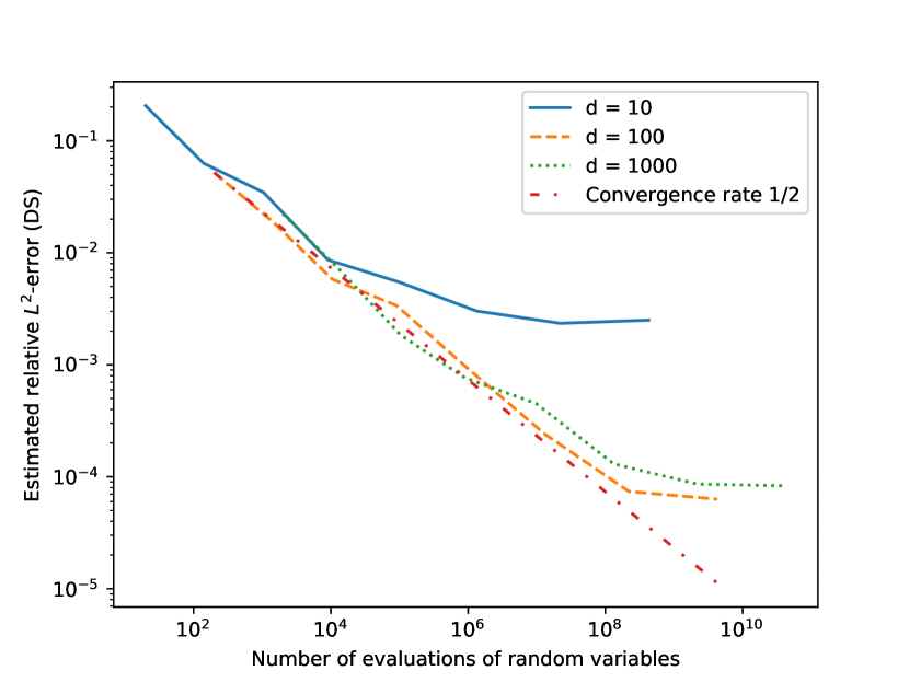
3.3 System of semilinear heat PDEs

In this subsection we apply the MLP approximation algorithm in (3) in Framework 1 above to the system of coupled semilinear heat PDEs in (8) below.

Assume Framework 1 and assume for all $t\in[0,T]$, $x,v\in\mathbb{R}^{d}$, $y=(y_{1},y_{2})\in\mathbb{R}^{2}$ that $k=2$, $T=1$, $f(x,y)=\big{(}\tfrac{y_{2}}{1+|y_{2}|^{2}},\tfrac{2y_{1}}{3}\big{)}$, $g(x)=\big{(}(2+\tfrac{2}{5}\left\|x\right\|^{2})^{-1},\log(\tfrac{1}{2}[1+\left\|x\right\|^{2}])\big{)}$, $\mu(x)=0$, and $\sigma(x)v=\sqrt{2}v$. Observe that this, (2), and (4) implies that for all $x\in\mathbb{R}^{d}$, $\theta\in\Theta$, $t\in[0,T]$, $s\in[t,T]$ it holds that $\mathbb{P}\big{(}X^{x,\theta}_{t,s}=x+\sqrt{2}(W^{\theta}_{s}-W^{\theta}_{t})\big{)}=1$ and

$$(\tfrac{\partial}{\partial t}u)(t,x)+(\Delta_{x}u)(t,x)+f\big{(}x,u(t,x)\big{)}=0.$$ (8)

In Table 3 we approximately present for $d\in\{10,100,1000\}$, $n\in\{1,2,\ldots,8\}$ one random realization of $V^{\theta}_{n,n,\infty}(0,0)$ (3 column in Table 3), the relative $L^{2}$-error $\frac{(\mathbb{E}[|V^{(0)}_{n,n,\infty}(0,0)-u(0,0)|^{2}])^{1/2}}{u(0,0)}$ (5 and 6 column in Table 3), the number of evaluations of one-dimensional random variables used to calculate one random realization of $V^{\theta}_{n,n,\infty}(0,0)$ (7 column in Table 3), and the runtime to calculate one random realization of $V^{\theta}_{n,n,\infty}(0,0)$ (8 column in Table 3). In Figure 3 we approximately plot for $d\in\{10,100,1000\}$, $n\in\{1,2,\ldots,8\}$ the relative $L^{2}$-error $\frac{(\mathbb{E}[|V^{(0)}_{n,n,\infty}(0,0)-u(0,0)|^{2}])^{1/2}}{u(0,0)}$ (5 and 6 column in Table 3) against the number of evaluations of one-dimensional random variables used to calculate one random realization of $V^{\theta}_{n,n,\infty}(0,0)$ (7 column in Table 3). The results in Table 3 and Figure 3 have been computed by means of C++ code LABEL:code in Section 4 below. For every $n\in\{1,2,\ldots,8\}$ for our approximative computations of the relative $L^{2}$-error $\frac{(\mathbb{E}[|V^{(0)}_{n,n,\infty}(0,0)-u(0,0)|^{2}])^{1/2}}{u(0,0)}$ (5 and 6 column in Table 3) the value $u(0,0)$ of the unknown exact solution in the relative $L^{2}$-error has been approximated by means of an average of 5 independent runs of the deep splitting approximation method in Beck et al. [3] (5 column in Table 3) and by means of an average of 5 independent evaluations of $V^{(0)}_{8,8,\infty}(0,0)$ (6 column in Table 3), respectively, and the expectation in the relative $L^{2}$-error has been approximated by means of Monte Carlo approximations involving 5 independent runs.

d	n	Result of MLP algorithm	Refe- rence solu- tions	Esti- mated relative $L^{2}$-error (DS)	Esti- mated relative $L^{2}$-error (MLP)	Evaluations of random variables	Run- time in sec- onds
10	1	(0.16714, 1.70085)		0.205522	0.205894	20	0.00028
10	2	(0.45134, 2.49508)	DS:	0.062991	0.064206	140	0.00011
10	3	(0.48243, 2.49320)	(0.47606,	0.034551	0.035524	1050	0.00050
10	4	(0.47085, 2.43225)	2.45101)	0.008637	0.009941	9080	0.00306
10	5	(0.47780, 2.44860)		0.005483	0.004484	98300	0.03706
10	6	(0.47539, 2.46088)	MLP:	0.003019	0.000984	1334340	0.57155
10	7	(0.47618, 2.45634)	(0.47621,	0.002347	0.000453	22032010	4.54895
10	8	(0.47627, 2.45705)	2.45726)	0.002504	0.000058	428332080	105.486
100	1	(0.01481, 4.41159)		0.051931	0.051942	200	0.00006
100	2	(0.21898, 4.72326)	DS:	0.019148	0.019169	1400	0.00012
100	3	(0.22044, 4.71319)	(0.21892,	0.005808	0.005762	10500	0.00081
100	4	(0.21877, 4.67656)	4.67722)	0.003379	0.003370	90800	0.00688
100	5	(0.21992, 4.68292)		0.000931	0.000895	983000	0.08848
100	6	(0.21905, 4.67801)	MLP:	0.000239	0.000199	13343400	1.42682
100	7	(0.21898, 4.67743)	(0.21895,	0.000074	0.000060	220320100	24.9459
100	8	(0.21893, 4.67757)	4.67750)	0.000063	0.000017	4283320800	828.779
1000	1	(0.00127, 6.88867)		0.022286	0.022261	2000	0.00013
1000	2	(0.14283, 6.87252)	DS:	0.006858	0.006795	14000	0.00063
1000	3	(0.14315, 6.94626)	(0.14273,	0.001836	0.001834	105000	0.00487
1000	4	(0.14244, 6.96112)	6.95587)	0.000763	0.000743	908000	0.04441
1000	5	(0.14278, 6.95906)		0.000451	0.000528	9830000	0.51808
1000	6	(0.14273, 6.95507)	MLP:	0.000130	0.000077	133434000	7.68460
1000	7	(0.14273, 6.95499)	(0.14274,	0.000086	0.000029	2203201000	208.043
1000	8	(0.14273, 6.95535)	6.95530)	0.000083	0.000010	42833208000	7867.29

Table 3: Numerical simulations for the MLP approximation algorithm in (3) in the case of the system of coupled semilinear heat PDEs in (8)

(a) Reference solutions computed by DS

(b) Reference solutions computed by MLP

Figure 3: Approximative plot of the relative $L^{2}$-error of the MLP approximation algorithm in (3) against the computational effort of the algorithm in the case of the system of coupled semilinear heat PDEs in (8).

3.4 Semilinear Black-Scholes PDEs

In this subsection we apply the MLP approximation algorithm in (3) in Framework 1 above to the semilinear Black-Scholes PDE in (10) below (cf. Black & Scholes [13]).

Assume Framework 1, let $\xi=(50,\ldots,50)\in\mathbb{R}^{d}$, assume for all $t\in[0,T]$, $x=(x_{1},\dots,x_{d})\in\mathbb{R}^{d}$, $y\in\mathbb{R}$ that $k=1$, $T=1$, $f(x,y)=\tfrac{y}{1+y^{2}}$, $g(x)=\log(\tfrac{1}{2}[1+\left\|x\right\|^{2}])$, $\mu(x)=x$, and $\sigma(x)=\operatorname{diag}(x_{1},\dots,x_{d})$, let $\langle\cdot,\cdot\rangle\colon(\cup_{q\in\mathbb{N}}(\mathbb{R}^{q}\times\mathbb{R}^{q}))\to\mathbb{R}$ be the standard scalar product, and let $e_{1},\dots,e_{d}\in\mathbb{R}^{d}$ satisfy that $e_{1}=(1,0,\dots,0)$, …, $e_{d}=(0,\dots,0,1)$. Combining this, (2), and (4) with Hutzenthaler et al. [42, Lemma 4.2] and the uniqueness property of solutions of stochastic differential equations (see, e.g., Klenke [48]) ensures that for all $x=(x_{1},\dots,x_{d})\in\mathbb{R}^{d}$, $\theta\in\Theta$, $t\in[0,T]$, $s\in[t,T]$ it holds that

$$\mathbb{P}\Big{(}X^{x,\theta}_{t,s}=\big{[}x_{1}\exp\big{(}\tfrac{(s-t)}{2}+\langle e_{1},W^{\theta}_{s}-W^{\theta}_{t}\rangle\big{)},\dots,x_{d}\exp\big{(}\tfrac{(s-t)}{2}+\langle e_{d},W^{\theta}_{s}-W^{\theta}_{t}\rangle\big{)}\big{]}\Big{)}=1$$ (9)

and

$$(\tfrac{\partial}{\partial t}u)(t,x)+f(x,u(t,x))+\tfrac{1}{2}\textstyle\sum\limits^{d}_{i=1}\Big{[}|x_{i}|^{2}\big{(}\tfrac{\partial^{2}}{\partial x_{i}\partial x_{i}}u\big{)}(t,x)\Big{]}+\textstyle\sum\limits_{i=1}^{d}\big{[}x_{i}(\tfrac{\partial}{\partial x_{i}}u)(t,x)\big{]}=0.$$ (10)

In Table 4 we approximately present for $d\in\{10,100,1000\}$, $n\in\{1,2,\ldots,8\}$ one random realization of $V^{\theta}_{n,n,\infty}(0,\xi)$ (3 column in Table 4), the relative $L^{2}$-error $\frac{(\mathbb{E}[|V^{(0)}_{n,n,\infty}(0,\xi)-u(0,\xi)|^{2}])^{1/2}}{u(0,\xi)}$ (5 and 6 column in Table 4), the number of evaluations of one-dimensional random variables used to calculate one random realization of $V^{\theta}_{n,n,\infty}(0,\xi)$ (7 column in Table 4), and the runtime to calculate one random realization of $V^{\theta}_{n,n,\infty}(0,\xi)$ (8 column in Table 4). In Figure 4 we approximately plot for $d\in\{10,100,1000\}$, $n\in\{1,2,\ldots,8\}$ the relative $L^{2}$-error $\frac{(\mathbb{E}[|V^{(0)}_{n,n,\infty}(0,\xi)-u(0,\xi)|^{2}])^{1/2}}{u(0,\xi)}$ (5 and 6 column in Table 4) against the number of evaluations of one-dimensional random variables used to calculate one random realization of $V^{\theta}_{n,n,\infty}(0,\xi)$ (7 column in Table 4). The results in Table 4 and Figure 4 have been computed by means of C++ code LABEL:code in Section 4 below. For every $n\in\{1,2,\ldots,8\}$ for our approximative computations of the relative $L^{2}$-error $\frac{(\mathbb{E}[|V^{(0)}_{n,n,\infty}(0,\xi)-u(0,\xi)|^{2}])^{1/2}}{u(0,\xi)}$ (5 and 6 column in Table 4) the value $u(0,\xi)$ of the unknown exact solution in the relative $L^{2}$-error has been approximated by means of an average of 5 independent runs of the deep splitting approximation method in Beck et al. [3] (5 column in Table 4) and by means of an average of 5 independent evaluations of $V^{(0)}_{8,8,\infty}(0,\xi)$ (6 column in Table 4), respectively, and the expectation in the relative $L^{2}$-error has been approximated by means of Monte Carlo approximations involving 5 independent runs.

d	n	Result of MLP algo- rithm	Refe- rence solu- tions	Esti- mated relative $L^{2}$-error (DS)	Esti- mated relative $L^{2}$-error (MLP)	Evaluations of random variables	Run- time in sec- onds
10	1	12.82440		0.056260	0.056265	20	0.00013
10	2	11.95260	DS:	0.032001	0.031983	140	0.00012
10	3	11.95160	11.98841	0.015161	0.015158	1050	0.00051
10	4	11.99310		0.005870	0.005885	9080	0.00329
10	5	11.99990		0.000666	0.000676	98300	0.03670
10	6	11.98910	MLP:	0.000100	0.000173	1334340	0.58832
10	7	11.98600	11.98736	0.000115	0.000059	22032010	4.92727
10	8	11.98750		0.000089	0.000012	428332080	116.666
100	1	14.10430		0.030842	0.030856	200	0.00006
100	2	14.75860	DS:	0.019049	0.019074	1400	0.00013
100	3	14.52930	14.68699	0.006795	0.006801	10500	0.00087
100	4	14.66750		0.001983	0.001971	90800	0.00760
100	5	14.68080		0.000416	0.000433	983000	0.09257
100	6	14.68710	MLP:	0.000089	0.000095	13343400	1.53685
100	7	14.68780	14.68754	0.000048	0.000027	220320100	27.5609
100	8	14.68760		0.000039	0.000009	4283320800	926.835
1000	1	16.92600		0.008389	0.008384	2000	0.00015
1000	2	17.24340	DS:	0.007540	0.007536	14000	0.00067
1000	3	17.11690	17.07785	0.001849	0.001844	105000	0.00521
1000	4	17.09480		0.000591	0.000600	908000	0.04907
1000	5	17.07760		0.000222	0.000221	9830000	0.59165
1000	6	17.07970	MLP:	0.000078	0.000087	133434000	8.48622
1000	7	17.07750	17.07766	0.000016	0.000015	2203201000	231.843
1000	8	17.07770		0.000011	0.000003	42833208000	8795.39

Table 4: Numerical simulations for the MLP approximation algorithm in (3) in the case of the Black-Scholes PDE in (10)

(a) Reference solutions computed by DS

(b) Reference solutions computed by MLP

Figure 4: Approximative plot of the relative $L^{2}$-error of the MLP approximation algorithm in (3) against the computational effort of the algorithm in the case of the Black-Scholes PDE in (10).

4 Source code

In this section we present the source code (see C++ code LABEL:code below) which was employed to produce the results in Subsections 3.1, 3.2, 3.3, and 3.4 above. All of the numerical simulations presented in Subsections 3.1, 3.2, 3.3, and 3.4 above were built and run on a system with an AMD Ryzen 9 3950X 16c/32t and 64 GB DDR4-3600 memory running Ubuntu 19.10. The provided source code uses the Eigen C++ Library (version 3.3.7) and the POSIX Threads API to allow for parallelism on modern multicore CPUs. It was compiled with the C++ compiler of the GNU Compiler Collection (version 7.5.0) with optimization level 3 (-O3). The different examples can be selected at compile time by providing a preprocessor symbol using the -D option to activate the corresponding preprocessor macro. Possible choices for the preprocessor symbol are ALLEN_CAHN (see Subsection 3.1), SINE_GORDON (see Subsection 3.2), PDE_SYSTEM (see Subsection 3.3), and SEMILINEAR_BS (see Subsection 3.4). For example, the source code for the Allen-Cahn example (see Subsection 3.1) was compiled using the command: g++ -DALLEN_CAHN -O3 -o mlp mlp.cpp -lpthread. Note that if the Eigen headers are not available system-wide the path has to be provided using the -I option in the command above.

⬇

1#define N_MAX 8

3#ifdef ALLEN_CAHN

#define eq_name ”Allen-Cahn_equation”

5#define rdim 1

#define g(x) ArrayXd tmp = ArrayXd::Zero(1, 1); tmp(0) = 1. / (2. + 2. / 5. * x.square().sum())

7#define X_sde(s, t, x, w) x + sqrt(2. * (t - s)) * w

#define fn(y) ArrayXd ret = ArrayXd::Zero(1, 1); double phi_r = std::min(4., std::max(-4., y(0))); ret(0) = phi_r - phi_r * phi_r * phi_r

9#endif

#ifdef SINE_GORDON

11#define eq_name ”Sine-Gordon_equation”

#define rdim 1

13#define g(x) ArrayXd tmp = ArrayXd::Zero(1, 1); tmp(0) = 1. / (2. + 2. / 5. * x.square().sum())

#define X_sde(s, t, x, w) x + sqrt(2. * (t - s)) * w

15#define fn(y) ArrayXd ret = ArrayXd::Zero(1, 1); ret(0) = sin(y(0))

#endif

17#ifdef SEMILINEAR_BS

#define eq_name ”Semilinear_Black-Scholes_equation”

19#define rdim 1

#define g(x) ArrayXd tmp = ArrayXd::Zero(1, 1); tmp(0) = log(0.5 * (1. + x.square().sum()))

21#define X_sde(s, t, x, w) x * ((t - s) / 2. + sqrt(t - s) * w).exp()

#define fn(y) ArrayXd ret = ArrayXd::Zero(1, 1); ret(0) = y(0) / (1. + y(0) * y(0))

23#endif

#ifdef PDE_SYSTEM

25#define eq_name ”Semilinear_PDE_system”

#define rdim 2

27#define X_sde(s, t, x, w) x + sqrt(2. * (t - s)) * w

#define g(x) ArrayXd tmp = ArrayXd::Zero(2, 1); tmp(0) = 1. / (2. + 2. / 5. * x.square().sum()); tmp(1) = log(0.5 * (1. + x.square().sum()))

29#define fn(y) ArrayXd ret = ArrayXd::Zero(2, 1); ret(0) = y(1) / (1. + y(1) * y(1)); ret(1) = 2. * y(0) / 3.

#endif

31

33#include <iostream>

#include <iomanip>

35#include <fstream>

#include <cstdint>

37#include <random>

#include <cmath>

39#include <ctime>

#include <thread>

41#include <chrono>

#include <eigen3/Eigen/Dense>

43

using Eigen::ArrayXd;

45

struct mlp_t {

47 uint8_t m;

uint8_t n;

49 uint8_t l;

uint16_t d;

51 ArrayXd x;

double s;

53 double t;

ArrayXd res;

55};

57

ArrayXd f(const ArrayXd &v);

59ArrayXd mlp_call(uint8_t m, uint8_t n, uint8_t l, uint16_t d, ArrayXd &x, double s, double t);

ArrayXd ml_picard(uint8_t m, uint8_t n, uint16_t d, ArrayXd &x, double s, double t, bool start_threads);

61void mlp_thread(mlp_t &mlp_args);

63int main() {

65 std::string s = eq_name;

std::cout << s << std::endl << std::endl << std::setprecision(8);

67

std::ofstream out_file;

69 out_file.open(s + ”_mlp.csv”);

out_file << ”d, T, n, ”;

71 for (uint8_t i=0; i < rdim; i++) {

out_file << ”result_” << (int)i << ”, ”;

73 }

out_file << ”elapsed_secs” << std::endl;

75

double T[1] = {1.};

77 uint16_t d[3] = {10, 100, 1000};

79 for (uint16_t j = 0; j < sizeof(d) / sizeof(d[0]); j++) {

for (uint8_t k = 0; k < sizeof(T) / sizeof(T[0]); k++) {

81 for (uint8_t n = 1; n <= N_MAX; n++) {

std::chrono::time_point<std::chrono::high_resolution_clock> start_time = std::chrono::high_resolution_clock::now();

83 #if defined(NONLINEAR_BS) || defined(SEMILINEAR_BS)

ArrayXd xi = ArrayXd::Constant(d[j], 1, 50.);

85 #else

ArrayXd xi = ArrayXd::Zero(d[j], 1);

87 #endif

ArrayXd result = ml_picard(n, n, d[j], xi, 0., T[k], true);

89

std::chrono::time_point<std::chrono::high_resolution_clock> end_time = std::chrono::high_resolution_clock::now();

91 double elapsed_secs = double(std::chrono::duration_cast<std::chrono::microseconds>(end_time - start_time).count()) / 1000. / 1000.;

std::cout << ”T: ” << T[k] << std::endl << ”d: ” << (int)d[j] << std::endl;

93 std::cout << ”n: ” << (int)n << std::endl << ”Result:” << std::endl << result << std::endl;

std::cout << ”Elapsed secs: ” << elapsed_secs << std::endl << std::endl;

95

out_file << (int)d[j] << ”, ” << T[k] << ”, ” << (int)n << ”, ”;

97 for (uint8_t i = 0; i < rdim; i++) {

out_file << result(i) << ”, ”;

99 }

out_file << elapsed_secs << std::endl;

101 }

}

103 }

105 out_file.close();

107 return 0;

}

109

ArrayXd f(const ArrayXd &v) {

111 fn(v);

return ret;

113}

115void mlp_thread(mlp_t &mlp_args) {

mlp_args.res = mlp_call(mlp_args.m, mlp_args.n, mlp_args.l, mlp_args.d, mlp_args.x, mlp_args.s, mlp_args.t);

117}

119ArrayXd mlp_call(uint8_t m, uint8_t n, uint8_t l, uint16_t d, ArrayXd &x, double s, double t) {

ArrayXd a = ArrayXd::Zero(rdim, 1);

121 ArrayXd b = ArrayXd::Zero(rdim, 1);

double r = 0.;

123 ArrayXd x2;

uint32_t num;

125 static thread_local std::mt19937 generator(128 + clock() + std::hash<std::thread::id>()(std::this_thread::get_id()));

static thread_local std::normal_distribution<> normal_distribution{0., 1.};

127 static thread_local std::uniform_real_distribution<double> uniform_distribution(0., 1.);

if (l < 2) {

129 num = (uint32_t)(pow(m, n - l) + 0.5);

for (uint32_t k = 0; k < num; k++) {

131 r = s + (t - s) * uniform_distribution(generator);

x2 = ArrayXd::NullaryExpr(d, [&](){ return normal_distribution(generator); });

133 x2 = X_sde(s, r, x, x2);

b += f(ml_picard(m, l, d, x2, r, t, false));

135 }

a += (t - s) * (b / ((double)num));

137 } else {

num = (uint32_t)(pow(m, n - l) + 0.5);

139 for (uint32_t k = 0; k < num; k++) {

r = s + (t - s) * uniform_distribution(generator);

141 x2 = ArrayXd::NullaryExpr(d, [&](){ return normal_distribution(generator); });

x2 = X_sde(s, r, x, x2);

143 b += (f(ml_picard(m, l, d, x2, r, t, l > m - 5)) - f(ml_picard(m, l - 1, d, x2, r, t, l > m - 5)));

}

145 a += (t - s) * (b / ((double)num));

}

147 return a;

}

149

ArrayXd ml_picard(uint8_t m, uint8_t n, uint16_t d, ArrayXd &x, double s, double t, bool start_threads) {

151

if (n == 0) return ArrayXd::Zero(rdim, 1);

153

ArrayXd a = ArrayXd::Zero(rdim, 1);

155 ArrayXd a2 = ArrayXd::Zero(rdim);

ArrayXd b = ArrayXd::Zero(rdim, 1);

157

double r = 0.;

159 std::thread threads[16];

mlp_t mlp_args[16];

161 ArrayXd x2;

uint32_t num;

163 static thread_local std::mt19937 generator(clock() + std::hash<std::thread::id>()(std::this_thread::get_id()));

static thread_local std::normal_distribution<> normal_distribution{0., 1.};

165 static thread_local std::uniform_real_distribution<double> uniform_distribution(0., 1.);

167

if (start_threads) {

169

for (uint8_t l = 0; l < n; l++) {

171 mlp_t mlp_arg;

mlp_arg.m = m;

173 mlp_arg.n = n;

mlp_arg.l = l;

175 mlp_arg.d = d;

mlp_arg.x = x.replicate(1, 1);

177 mlp_arg.s = s;

mlp_arg.t = t;

179 mlp_arg.res = 0.;

mlp_args[l] = mlp_arg;

181 threads[l] = std::thread(mlp_thread, std::ref(mlp_args[l]));

}

183

num = (uint32_t)(pow(m, n) + 0.5);

185 for (uint32_t k = 0; k < num; k++) {

x2 = ArrayXd::NullaryExpr(d, [&](){ return normal_distribution(generator); });

187 x2 = X_sde(s, t, x, x2);

g(x2);

189 a2 += tmp;

}

191

a2 /= (double)num;

193

for (uint8_t l = 0; l < n; l++) {

195 threads[l].join();

a += mlp_args[l].res;

197 }

199 } else {

201 for (uint8_t l = 0; l < std::min(n, (uint8_t)2); l++) {

b = ArrayXd::Zero(rdim, 1);

203 num = (uint32_t)(pow(m, n - l) + 0.5);

for (uint32_t k = 0; k < num; k++) {

205 r = s + (t - s) * uniform_distribution(generator);

x2 = ArrayXd::NullaryExpr(d, [&](){ return normal_distribution(generator); });

207 x2 = X_sde(s, r, x, x2);

b += f(ml_picard(m, l, d, x2, r, t, false));

209 }

a += (t - s) * (b / ((double)num));

211 }

213 for (uint8_t l = 2; l < n; l++) {

b = ArrayXd::Zero(rdim, 1);

215 num = (uint32_t)(pow(m, n - l) + 0.5);

for (uint32_t k = 0; k < num; k++) {

217 r = s + (t - s) * uniform_distribution(generator);

x2 = ArrayXd::NullaryExpr(d, [&](){ return normal_distribution(generator); });

219 x2 = X_sde(s, r, x, x2);

b += (f(ml_picard(m, l, d, x2, r, t, false)) - f(ml_picard(m, l - 1, d, x2, r, t, false)));

221 }

a += (t - s) * (b / ((double)num));

223 }

225 num = (uint32_t)(pow(m, n) + 0.5);

for (uint32_t k = 0; k < num; k++) {

227 x2 = ArrayXd::NullaryExpr(d, [&](){ return normal_distribution(generator); });

x2 = X_sde(s, t, x, x2);

229 g(x2);

a2 += tmp;

231 }

233 a2 /= (double)num;

235 }

237 return a + a2;

}

C++ code 1: Source code for Subsections 3.1, 3.2, 3.3, and 3.4

References

- [1] Barone, A., Esposito, F., Magee, C., and Scott, A. Theory and applications of the sine-Gordon equation. La Rivista del Nuovo Cimento (1971-1977) 1, 2 (1971), 227–267.
- [2] Bartels, S. Numerical Methods for Nonlinear Partial Differential Equations. Springer International Publishing, 2015.
- [3] Beck, C., Becker, S., Cheridito, P., Jentzen, A., and Neufeld, A. Deep splitting method for parabolic PDEs. arXiv:1907.03452 (2019), 40 pages.
- [4] Beck, C., Becker, S., Grohs, P., Jaafari, N., and Jentzen, A. Solving stochastic differential equations and Kolmogorov equations by means of deep learning. arXiv:1806.00421 (2018), 56 pages.
- [5] Beck, C., E, W., and Jentzen, A. Machine learning approximation algorithms for high-dimensional fully nonlinear partial differential equations and second-order backward stochastic differential equations. J. Nonlinear Sci. 29, 4 (2019), 1563–1619.
- [6] Beck, C., Gonon, L., and Jentzen, A. Overcoming the curse of dimensionality in the numerical approximationof high-dimensional semilinear elliptic partial differential equations. arXiv:2003.00596 (2020), 50 pages.
- [7] Beck, C., Hornung, F., Hutzenthaler, M., Jentzen, A., and Kruse, T. Overcoming the curse of dimensionality in the numerical approximation of Allen–Cahn partial differential equations via truncated full-history recursive multilevel Picard approximations. arXiv:1907.06729 (2019), 31 pages.
- [8] Becker, S., Cheridito, P., and Jentzen, A. Deep optimal stopping. J. Mach. Learn. Res. 20 (2019), Paper No. 74, 25.
- [9] Becker, S., Cheridito, P., and Jentzen, A. Pricing and hedging american-style options with deep learning. arXiv:1912.11060 (2019), 12 pages.
- [10] Becker, S., Cheridito, P., Jentzen, A., and Welti, T. Solving high-dimensional optimal stopping problems using deep learning. arXiv:1908.01602 (2019), 42 pages.
- [11] Berg, J., and Nyström, K. A unified deep artificial neural network approach to partial differential equations in complex geometries. Neurocomputing 317 (2018), 28–41.
- [12] Berner, J., Grohs, P., and Jentzen, A. Analysis of the generalization error: Empirical risk minimization over deep artificial neural networks overcomes the curse of dimensionality in the numerical approximation of Black-Scholes partial differential equations. arXiv:1809.03062 (2018), 35 pages. Accepted in J. Sci. Comput.
- [13] Black, F., and Scholes, M. The pricing of options and corporate liabilities. Journal of political economy 81, 3 (1973), 637–654.
- [14] Chan-Wai-Nam, Q., Mikael, J., and Warin, X. Machine learning for semi linear PDEs. arXiv:1809.07609 (2018), 38 pages.
- [15] Chen, Y., and Wan, J. W. Deep neural network framework based on backward stochastic differential equations for pricing and hedging american options in high dimensions. arXiv:1909.11532 (2019), 35 pages.
- [16] Chiaramonte, M., and Kiener, M. Solving differential equations using neural networks. Machine Learning Project (2013).
- [17] Coleman, S. Quantum sine-Gordon equation as the massive Thirring model. Phys. Rev. D 11 (1975), 2088–2097.
- [18] Dockhorn, T. A discussion on solving partial differential equations using neural networks. arXiv:1904.07200 (2019), 9 pages.
- [19] E, W., Han, J., and Jentzen, A. Deep learning-based numerical methods for high-dimensional parabolic partial differential equations and backward stochastic differential equations. Communications in Mathematics and Statistics 5, 4 (2017), 349–380.
- [20] E, W., Hutzenthaler, M., Jentzen, A., and Kruse, T. Multilevel Picard iterations for solving smooth semilinear parabolic heat equations. arXiv:1607.03295 (2016), 18 pages.
- [21] E, W., Hutzenthaler, M., Jentzen, A., and Kruse, T. On multilevel Picard numerical approximations for high-dimensional nonlinear parabolic partial differential equations and high-dimensional nonlinear backward stochastic differential equations. J. Sci. Comput. 79, 3 (2019), 1534–1571.
- [22] E, W., and Yu, B. The deep Ritz method: a deep learning-based numerical algorithm for solving variational problems. Commun. Math. Stat. 6, 1 (2018), 1–12.
- [23] Elbrächter, D., Grohs, P., Jentzen, A., and Schwab, C. DNN Expression Rate Analysis of High-dimensional PDEs: Application to Option Pricing. arXiv:1809.07669 (2018), 50 pages.
- [24] Farahmand, A., Nabi, S., and Nikovski, D. Deep reinforcement learning for partial differential equation control. In 2017 American Control Conference (ACC) (Seattle, WA, 2017), pp. 3120–3127.
- [25] Feng, X., and Prohl, A. Numerical analysis of the Allen-Cahn equation and approximation for mean curvature flows. Numerische Mathematik 94, 1 (2003), 33–65.
- [26] Fujii, M., Takahashi, A., and Takahashi, M. Asymptotic Expansion as Prior Knowledge in Deep Learning Method for High dimensional BSDEs. Asia-Pacific Financial Markets 26, 3 (September 2019), 391–408.
- [27] Giles, M. B., Jentzen, A., and Welti, T. Generalised multilevel picard approximations. arXiv:1911.03188 (2019), 61 pages.
- [28] Gonon, L., Grohs, P., Jentzen, A., Kofler, D., and Šiška, D. Uniform error estimates for artificial neural network approximations for heat equations. arXiv:1911.09647 (2019), 70 pages.
- [29] Goudenege, L., Molent, A., and Zanette, A. Machine learning for pricing american options in high dimension. arXiv:1903.11275 (2019), 11 pages.
- [30] Grohs, P., Hornung, F., Jentzen, A., and von Wurstemberger, P. A proof that artificial neural networks overcome the curse of dimensionality in the numerical approximation of Black-Scholes partial differential equations. arXiv:1809.02362 (2018), 124 pages. To appear in Mem. Amer. Math. Soc.
- [31] Grohs, P., Hornung, F., Jentzen, A., and Zimmermann, P. Space-time error estimates for deep neural network approximations for differential equations. arXiv:1908.03833 (2019), 86 pages.
- [32] Grohs, P., Jentzen, A., and Salimova, D. Deep neural network approximations for monte carlo algorithms. arXiv:1908.10828 (2019), 45 pages.
- [33] Hairer, M., and Hao, S. The dynamical sine-Gordon model. Communications in Mathematical Physics 341 (2016), 933–989.
- [34] Han, J., Jentzen, A., and E, W. Solving high-dimensional partial differential equations using deep learning. Proceedings of the National Academy of Sciences 115, 34 (2018), 8505–8510.
- [35] Han, J., and Long, J. Convergence of the Deep BSDE Method for Coupled FBSDEs. arXiv:1811.01165 (2018), 26 pages.
- [36] He, J., Li, L., Xu, J., and Zheng, C. Relu deep neural networks and linear finite elements. arXiv:1807.03973 (2018), 50 pages.
- [37] Henry-Labordere, P. Deep primal-dual algorithm for BSDEs: Applications of machine learning to CVA and IM. Available at SSRN 3071506 (2017).
- [38] Huré, C., Pham, H., and Warin, X. Some machine learning schemes for high-dimensional nonlinear PDEs. arXiv:1902.01599 (2019), 33 pages.
- [39] Hutzenthaler, M., Jentzen, A., and Kruse, T. Overcoming the curse of dimensionality in the numerical approximation of parabolic partial differential equations with gradient-dependent nonlinearities. arXiv:1912.02571 (2019), 33 pages.
- [40] Hutzenthaler, M., Jentzen, A., Kruse, T., and Nguyen, T. A. A proof that rectified deep neural networks overcome the curse of dimensionality in the numerical approximation of semilinear heat equations. SN Partial Differ. Equ. Appl. 1, 10 (2020).
- [41] Hutzenthaler, M., Jentzen, A., Kruse, T., Nguyen, T. A., and von Wurstemberger, P. Overcoming the curse of dimensionality in the numerical approximation of semilinear parabolic partial differential equations. arXiv:1807.01212 (2018), 30 pages.
- [42] Hutzenthaler, M., Jentzen, A., and Wurstemberger, P. Overcoming the curse of dimensionality in the approximative pricing of financial derivatives with default risks. arXiv:1903.05985 (2019), 71 pages. Accepted in Electron. J. Probab.
- [43] Hutzenthaler, M., and Kruse, T. Multi-level Picard approximations of high-dimensional semilinear parabolic differential equations with gradient-dependent nonlinearities. arXiv:1711.01080 (2017), 19 pages.
- [44] Jacquier, A., and Oumgari, M. Deep PPDEs for rough local stochastic volatility. arXiv:1906.02551 (2019), 21 pages.
- [45] Jentzen, A., Salimova, D., and Welti, T. A proof that deep artificial neural networks overcome the curse of dimensionality in the numerical approximation of Kolmogorov partial differential equations with constant diffusion and nonlinear drift coefficients. arXiv:1809.07321 (2018), 48 pages.
- [46] Jianyu, L., Siwei, L., Yingjian, Q., and Yaping, H. Numerical solution of elliptic partial differential equation using radial basis function neural networks. Neural Networks 16, 5-6 (2003), 729–734.
- [47] Khoo, Y., Lu, J., and Ying, L. Solving parametric PDE problems with artificial neural networks. arXiv:1707.03351 (2017), 17 pages.
- [48] Klenke, A. Probabilitly Theory, 2 ed. Universitext. Springer-Verlag London Ltd., 2014.
- [49] Kutyniok, G., Petersen, P., Raslan, M., and Schneider, R. A theoretical analysis of deep neural networks and parametric pdes. arXiv:1904.00377 (2019), 40 pages.
- [50] Lagaris, I. E., Likas, A., and Fotiadis, D. I. Artificial neural networks for solving ordinary and partial differential equations. IEEE transactions on neural networks 9, 5 (1998), 987–1000.
- [51] Lee, H., and Kang, I. S. Neural algorithm for solving differential equations. Journal of Computational Physics 91, 1 (1990), 110–131.
- [52] Long, Z., Lu, Y., Ma, X., Dong, B., and null Pde-Net. PDE-Net: Learning PDEs from Data. arXiv:1710.09668 (2017), 15 pages.
- [53] Lye, K. O., Mishra, S., and Ray, D. Deep learning observables in computational fluid dynamics. Journal of Computational Physics (2020), 109339.
- [54] Magill, M., Qureshi, F., and de Haan, H. Neural networks trained to solve differential equations learn general representations. In Advances in Neural Information Processing Systems (2018), pp. 4071–4081.
- [55] Meade Jr, A. J., and Fernandez, A. A. The numerical solution of linear ordinary differential equations by feedforward neural networks. Mathematical and Computer Modelling 19, 12 (1994), 1–25.
- [56] Nabian, M. A., and Meidani, H. A deep neural network surrogate for high-dimensional random partial differential equations. arXiv:1806.02957 (2018), 23 pages.
- [57] Nüsken, N., and Richter, L. Solving high-dimensional Hamilton-Jacobi-Bellman PDEs using neural networks: perspectives from the theory of controlled diffusions and measures on path space. arXiv:2005.05409 (2020), 40 pages.
- [58] Pham, H., and Warin, X. Neural networks-based backward scheme for fully nonlinear PDEs. arXiv:1908.00412 (2019), 15 pages.
- [59] Raissi, M. Deep hidden physics models: Deep learning of nonlinear partial differential equations. The Journal of Machine Learning Research 19, 1 (2018), 932–955.
- [60] Raissi, M. Forward-backward stochastic neural networks: Deep learning of high-dimensional partial differential equations. arXiv:1804.07010 (2018), 17 pages.
- [61] Ramuhalli, P., Udpa, L., and Udpa, S. S. Finite-element neural networks for solving differential equations. IEEE transactions on neural networks 16, 6 (2005), 1381–1392.
- [62] Reisinger, C., and Zhang, Y. Rectified deep neural networks overcome the curse of dimensionality for nonsmooth value functions in zero-sum games of nonlinear stiff systems. arXiv:1903.06652 (2019), 34 pages.
- [63] Sirignano, J., and Spiliopoulos, K. DGM: A deep learning algorithm for solving partial differential equations. Journal of Computational Physics 375 (2018), 1339–1364.
- [64] Uchiyama, T., and Sonehara, N. Solving inverse problems in nonlinear pdes by recurrent neural networks. In IEEE International Conference on Neural Networks (1993), IEEE, pp. 99–102.