Self-Updating Models with Error Remediation

Abstract

Many environments currently employ machine learning models for data processing and analytics that were built using a limited number of training data points. Once deployed, the models are exposed to significant amounts of previously-unseen data, not all of which is representative of the original, limited training data. However, updating these deployed models can be difficult due to logistical, bandwidth, time, hardware, and/or data sensitivity constraints. We propose a framework, Self-Updating Models with Error Remediation (SUMER), in which a deployed model updates itself as new data becomes available. SUMER uses techniques from semi-supervised learning and noise remediation to iteratively retrain a deployed model using intelligently-chosen predictions from the model as the labels for new training iterations. A key component of SUMER is the notion of error remediation as self-labeled data can be susceptible to the propagation of errors. We investigate the use of SUMER across various data sets and iterations. We find that self-updating models (SUMs) generally perform better than models that do not attempt to self-update when presented with additional previously-unseen data. This performance gap is accentuated in cases where there is only limited amounts of initial training data. We also find that the performance of SUMER is generally better than the performance of SUMs, demonstrating a benefit in applying error remediation. Consequently, SUMER can autonomously enhance the operational capabilities of existing data processing systems by intelligently updating models in dynamic environments.

Justin E. Doak, Michael R. Smith, Joey B. Ingram, ”Self-updating models with error remediation,” Proc. SPIE 11413, Artificial Intelligence and Machine Learning for Multi-Domain Operations Applications II, 114131W (18 May 2020); doi: 10.1117/12.2563843

Copyright 2020 Society of PhotoOptical Instrumentation Engineers. One print or electronic copy may be made for personal use only. Systematic reproduction and distribution, duplication of any material in this paper for a fee or for commercial purposes, or modification of the content of the paper are prohibited.

1 INTRODUCTION

Self-Updating Models with Error Remediation (SUMER) is concerned with autonomously updating deployed machine learning models as data naturally or adversarially drifts over time in order to maintain desired performance. Figure 1 illustrates the continuous updating process employed by the SUMER framework overlaid with a more traditional machine learning deployment. The black lines represent a traditional machine learning process and the blue lines represent the SUM/SUMER framework.

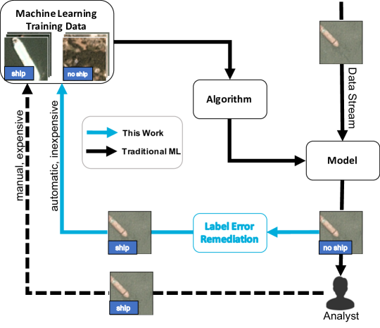
Figure 1: SUMER versus traditional machine learning for an example ship detection problem

The main difference shown in Fig. 1 is the mechanism used to keep a model up-to-date with the observed data. In traditional machine learning, a human typically labels instances from the data stream, which are then inserted into the training data and the machine learning model is updated. This process is depicted with the dashed line as it is often not done in practice due to the labor-intensive cost associated with manual labeling. The SUMER framework proposes to eliminate this bottleneck by using the current model’s predictions as labels after correcting any potential errors.

However, in order to fully implement the proposed SUMER framework, access to the following resources are required:

• Training data - the set of annotated (i.e., labeled) data used to derive the machine learning model to perform the desired task. For example, in the ship detection example, the set of images and corresponding label for each image (i.e., “ship” or “no ship”) constitute the training data. This data will be used to develop the self-updating and label correction models.

• Machine learning algorithm - the algorithm and implementation used to induce a model that can be deployed.

• Access to data stream - samples of data from the deployed environment that were not observed in the training data. The data stream should be in the same format as the training data (e.g., the same feature space) or convertible to the same format. For experimentation, ground-truth labels for these samples would also be desirable to evaluate performance.

• Access to production system - a way to deploy the SUMER framework and “hook” into an existing production system will also be necessary.

A checklist of currently defined requirements will be discussed in Sec. 1.2.

1.1 Relevant Machine Learning Scenarios

SUMER is an amalgam of several machine learning scenarios in an attempt to reduce or eliminate common issues that arise when utilizing machine learning in practical environments. A list of relevant scenarios and their definitions follows (along with some relevant references in open research):

• Active Learning [1] - exploit what the model thinks that it doesn’t know. This attempts to reduce the number of labels needed to update a model by allowing the model to query an oracle, usually a human expert, for labels on selected samples from the data stream.

• Concept Drift Detection [2] - detect a shift in the distribution of the data, which is typically detrimental to model performance. This could be a change in the data associated with known classes or the introduction of one or more previously unknown classes.

• Domain Adaptation [3]- adapt a model to a distribution shift between the training data used to induce a model and the data stream to which the model is applied. This typically assumes that the features used in the training data and data stream are equivalent (i.e., the input(s) to the model will be the same).

• Feature Augmentation [4, 5] - add or modify the features (i.e., input(s)) that the model uses to make its predictions in order to improve performance on the desired task. For example, new features can be created based on the outputs of auxiliary models (e.g., outlier detection).

• Learning with Label Noise [6, 7] - induce a well-performing model given that some of the data is known to be mislabeled. This can be done by detecting potential errors and removing those samples, changing their labels, or by weighting those samples accordingly.

• Model Shift Detection [8] - determine when a deployed model is not performing as expected, but do not attempt to correct performance. Typically accomplished by monitoring the output of the model and detecting shifts in its distribution.

• Semi-supervised Learning [9]- exploit what the model thinks it knows. That is, assume that samples in the data stream are correctly labeled if the model is confident in its predictions. As in active learning, the goal is to reduce the number of labels needed from an oracle, which is an expensive process.

1.2 Comparison of Learning Scenarios

As the aforementioned learning scenarios are related, their requirements can be similarly defined. Table 1 lists the necessary requirements for each of the scenarios. By determining what is available for a potential application and comparing with Tab. 1, the matching scenarios could potentially be utilized. All that remains would be to decide if the problem solved by the matching scenarios is of utility to the transition partner before moving forward.

In summary, although as defined SUMER requires access to several resources to be effective, the framework can be adapted to solve a large variety of related problems, based on the needs of the application and what can currently be provided.

Table 1: Comparison of various relevant machine learning scenarios to SUMER

	SUMER	Traditional ML	Active Learning	Concept Drift Detection	Domain Adaptation	Feature Augmentation	Learning w/ Label Noise	Model Shift Detection	Semi-superivsed Learning
Training Data	✓	✓	✓	✓	✓	✓	✓		✓
Data Stream	✓	✓	✓	✓	✓	✓	✓		✓
Output of Deployed Model on Data Stream	✓	✓	✓					✓	✓
Mechanism to Update Deployed Model	✓	✓	✓		✓		✓		✓
Self-prediction Mechanism to Label Data Stream	✓								✓
Label Error Detection / Correction	✓						✓
Analyst / Oracle to Label Data Stream		✓	✓

1.3 Synopsis

In order to advance an autonomous machine learning framework that self-adapts to changing environments, the most immediate problem that was identified was that of error propagation in SUMs. If models are to be self-updated in practical, deployed environments with minimal human intervention, then these models need to be able to identify and self-correct mistakes. To successfully address this problem, the task was divided into two main thrusts: 1) demonstrate the benefits of self-updating and 2) demonstrate the benefits of self-updating with error remediation

The remainder of the paper is as follows. Section 2 defines the problem and provides more intuition surrounding it. Section 4 identifies and summarizes open research that is relevant to this work. It also provides an initial taxonomy for SUMs and remediation techniques. Section 3 describes the experiments that were performed during the course of this research in order to understand SUMs and SUMER. This section also describes some issues that were identified with utilizing these models in practical environments. Section 5 concludes the report and provides proposed next stages for this research.

2 PROBLEM FORMULATION

The problem of self-updating models can be seen in the following example. Assume that the task is to differentiate between black and white points. In this setting, we are assuming that more data will arrive as the model is deployed. Given a labeled point from each class, a decision boundary can be inferred as illustrated in Fig. 2a. Given a new point, the gray point in Fig. 2b, how should that new point be labeled? Without further context, the best that the model can do is categorize the point as belonging to the “white” class.

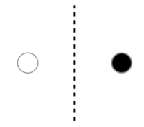
(a)

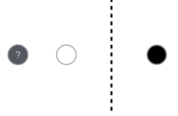
(b)

Figure 2: Illustrative example of traditional machine learning (a) Given two labeled data points (with or without additional unlabeled data points), a decision boundary is inferred. (b) When a new unlabeled data point is presented, lacking any additional information, the inferred decision boundary is the same, dictating the prediction of the new point[10].

Now, under the assumption that more unlabeled data is constantly being observed, that data can be leveraged to update the model as illustrated in Fig. 3a-d. This examples illustrates what happens if the data is updated in batches based on intermediate self-updating of the nearest points. If all of the data were labeled at once based on proximity to the original labeled data points, then the classification boundary would have appeared similar to the original decision boundary in Fig. 2a.

(a)

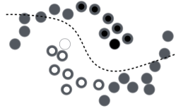
(b)

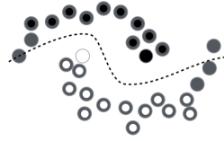
(c)

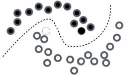
(d)

Figure 3: Illustrative example of iteratively labeling unlabeled data points and retraining an algorithm to infer a decision boundary[10].

By labeling the data in a strategic manner, the correct decision boundary could be inferred. Self-labeling will often use the labels from a model about which it is most confident. Confidence in many models is estimated by the distances from a decision boundary. However, in examining the model, there are different areas of uncertainty that should be taken into account when performing self-labeling as illustrated in Fig. 4 representing a decision boundary (the solid blue line) between the green and yellow class. These are represented by the gray box in the middle of the decision boundary and the blue-black gradient extending toward each side. The source of uncertainty of the gray box is from the overlapping points from differing classes. The source of uncertainty in the blue-black gradient triangles is because there is a lack of data on those areas. Thus, even if the model is confident about a prediction (e.g. the data point is far away from the decision boundary), if the data point is not represented by the training data, the confidence should be low.

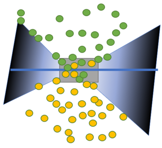
Figure 4: Notional illustration of uncertainty of a machine learning model discriminating between green and yellow. The gray box represents uncertainty in the feature space as the classes overlap. The blue-black gradient triangles represent uncertainty due to a lack of training data in that portion of the input space.

The end goal, therefore, is to autonomously update a learned model using its own output on new data points where: 1) the training data does not cover and 2) there is high confidence that the model can extrapolate or generalize to that new area. In the streaming sense, we aim to remediate incorrect predictions so that errors are not propagated in future iterations and we would also like to detect concept drift and novel concepts. The novelty in the proposed research lies in the fusion of multiple algorithms in deployed environments that adapt over time. Most of the open research assumes a fixed dataset or does not address the issue of multiple rounds of self-updating. However, there are several outstanding issues not considered during the course of this research. For example, this work does not attempt to address drift in the underlying concepts associated with the learning task. Section 5 provides more detail on remaining research gaps and potential solutions.

3 Experimental Methodology and Results

In this section, we will describe the various datasets that were used for experimentation, along with the experimental set up and results obtained for this data. Additionally, we will discuss some of the conclusions that we have drawn from the outcomes of our experiments. Finally, we will describe some potential issues that were discovered over the course of our research involving the use of self-updating models and label error remediation in practice.

3.1 Datasets

Before discussing the various experiments that were performed, it is useful to understand the datasets that were used. A few datasets were utilized in order to ensure that any conclusions obtained from our experiments would generalize to similar machine learning problems.

3.1.1 Synthetic framework

In machine learning research, it is often useful to perform experiments on synthetically-generated data. By using synthetic data with known properties, it allows for the understanding of algorithms without having to account for the various complexities associated with real-world data, which are often unknown or difficult to summarize. Therefore, a synthetic data generation and label noise insertion framework was developed for experimentation purposes. This framework proved very useful for determining potential practical issues associated with self-updating models and label error remediation techniques.

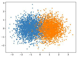
(a) Two Gaussians

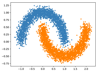
(b) Two Moons

Figure 5: Examples of synthetically-generated data for two-class (binary) machine learning problems

Figure 5 shows data that was generated by the developed framework for two different binary machine learning problems. Here, the goal of the model is to categorize a data point as blue or orange. The features for each point are simply the coordinates in two-dimensional space. The first example, shown in Fig. 5a, generates data from two separate multivariate Normal distributions. The second example, shown in Fig. 5b, generates data points for each of two overlapping “moons”. In this case, the optimal classifier is nonlinear.

3.1.2 Ships in satellite imagery

The Kaggle “Ships in Satellite Imagery” dataset [11] is comprised of a collection of $80\times 80$ red-green-blue (RGB) chips that were extracted from satellite images provided by Planet. The goal of this dataset is to induce a model that can detect whether or not a given chip contains a ship (i.e., predict “ship” or “no ship”). The features for this problem are the pixel intensities in the red, green, and blue channels for each of the pixels, which are represented as integers in $[0,255]$. Given that there are three channels and $80\times 80$ pixels, the resulting feature space is quite large and each chip is represented by 19,200 integers. Figure 6 shows an example from each of the two classes, along with the histograms of pixel intensities.

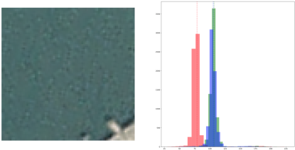
(a) No Ship

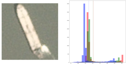
(b) Ship

Figure 6: Examples of images for the ship detection problem and their respective RGB histograms

Originally, there were 1,000 examples of ships and 3,000 examples of non-ships, for a total of 4,000 image chips in the dataset. However, the non-ship class is composed of 1,000 land-cover chips, 1000 partial ships, and 1,000 commonly misclassified chips that do not contain ships. We consider the 1,000 partial ships and 1,000 commonly misclassified chips to be associated with concept drift and were therefore left out of some of the experiments. For relevant experimental results, we will explicitly mention when these chips were held out.

Additionally, for future experiments involving concept drift, it would be useful to re-label the partial ships to be a part of the “ship” class. In this instance, this re-labeling procedure would be of more interest from a practical perspective as the chip still contains a part of a ship. However, as concept drift was not considered for our initial experiments, this distinction is not required.

3.2 Experiments on Synthetic Data

The first experiment aimed to demonstrate the benefit of SUMs on synthetic data, specifically the Two Moons dataset. Figure 7 shows the result of a SUM applied to this data using label spreading [12]. The left side of the figure shows the data. The unlabeled data is shown by the gray points and the labeled points are shown by the blue/orange points. The right side of the figure shows the learned model. With an accuracy of over $95\%$, it is clear that label spreading is able to learn a good model with only a few labeled points. However, this experiment only shows a SUM when all of the unlabeled data is known in advance (i.e., a single round of self-updating).

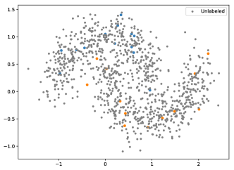
(a) Two Moons with only a few samples labeled

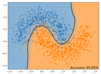
(b) Resulting SUM predictions

Figure 7: Illustration of SUMs on Two Moons dataset

Therefore, the next experiment investigated the performance of SUMs over multiple rounds of self-updating. Figure 8 shows the performance of a SUM over a simulated stream. The algorithm is provided with an initial labeled dataset as in the experiment with the single round of self-updating. Initially, twenty points are labeled. With only a single round of self-updating, all the remaining unlabeled data is self-labeled by the model and then the model is updated. However, for multiple rounds of self-updating, we simulate a stream by continuing to draw new instances from the same distribution and periodically updating the model with this new data. In this case, the SUM provides a clear benefit of over $2\%$ in accuracy (the orange curve) compared to an initial model that does not self-update (the blue curve). The green curve provides an estimate of the upper bound performance by allowing the algorithm to update with the correctly labeled data (i.e., it has access to all of the labeled data at once).

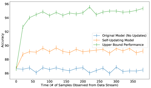
Figure 8: Benefit of SUMs on a simulated stream over time

The final experiment that was performed on the synthetic data involved self-updating with error remediation (SUMER). Figure 9 shows the models that were learned from data that had $20\%$ label noise. The label noise was introduced by randomly flipping labels. It can be seen that the SUMER model provides an approximately $5\%$ increase in accuracy. Both models utilized the label spreading algorithm, but in the case of SUMER, a parameter was changed to allow provided labels to be corrected, based on the optimization procedure derived by the algorithm.

The aforementioned experiments demonstrate the benefit of SUMs/SUMER on synthetic data, but these methods need to be vetted in more realistic settings. Therefore, we performed similar experiments on more realistic data.

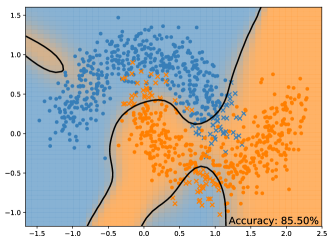
(a) SUM

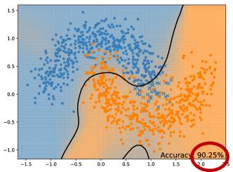
(b) SUMER

Figure 9: The benefit of SUMER in the presence of label noise

3.3 Experiments on Real-World Data

As mentioned in Sec. 3.1.2, a realistic dataset involving detecting ships versus landcover has been collected and annotated. An initial experiment was conducted to demonstrate the benefit of SUMs. For this experiment, the original, unmodified Kaggle data was used (1000 ships and 3000 non-ships). For our model, we used Random Forests [13] in a self-updating manner. Figure 10 shows the performance as a function of the amount of data that is initially labeled. The $x$-axis shows the fraction of data that has been labeled. The algorithm labels the unlabeled data using the SUM and the performance accuracy is estimated based on a held-out set of instances. When there is only a small amount of data initially labeled ($\approx 5$-$10\%$), SUMs provide an approximately $10\%$ increase in performance. As the amount of initially labeled data increases, the performance converges to the performance of the model with access to all of the labels, as expected. However, in practice, the more data that is labeled, the more labor-intensive the process is, which means that the model is more costly to create.

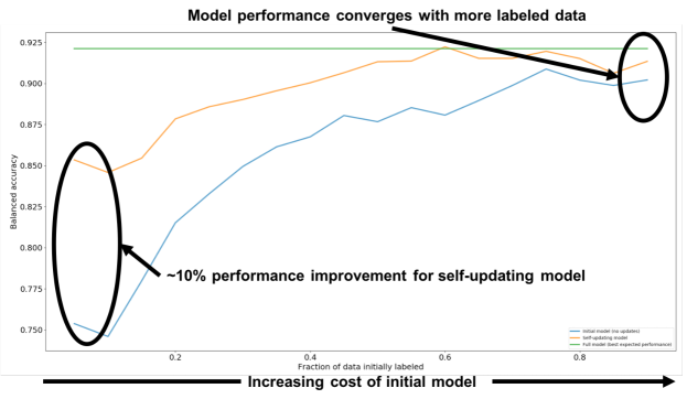
Figure 10: Benefit of SUMs on Kaggle ships data

The final experiment that was conducted involved evaluating the performance of SUMER on a simulated stream of realistic data. In this case, the data without drift was used (1000 ships and 1000 non-ships). However, $20\%$ label noise was injected into the initial training data in order to evaluate the effect on the performance (the true labels were used when estimating performance). The stream was simulated by sampling (without replacement) instances from the full set of data in predetermined windows. For this experiment, Random Forests with Rank Pruning [14] was used for the SUMER algorithm.

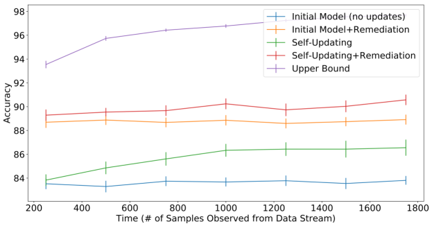
Figure 11: Benefit of SUMER on Kaggle ships data with $20\%$ label noise

Figure 11 shows the results of this experiment. As expected, both SUM and SUMER perform better than an initial model that does not update. SUMER comes the closest to the upper bound performance (i.e., the model with full access to the correct labels). It should be noted that the reason there is only a small increase in accuracy observed between the initial model with error remediation (the orange curve) and SUMER (the red curve) is likely due to the model coupling problem, which will be discussed in Sec. 3.5.

It seems that SUMs and SUMER are potentially very useful for performing well in dynamic, label-constrained environments. However, there are still some potential issues that should be discussed before utilizing them in practice.

3.4 Potential Issues with SUMs in Practice

One issue with using SUMs in practice surrounds the instances that are initially labeled, which can drastically affect the overall performance of the resulting model. Figure 12 demonstrates this issue. The data is sampled from the same distribution as in Fig. 7, but the instances that are labeled are different, which results in an approximately $15\%$ decrease in performance. This problem is related to the problem of concept drift [2]. Areas of the data distribution are not labeled, which makes it difficult for the algorithm to determine a correct labeling in those areas of the feature space. This difficulty, in turn, affects the potential performance of the algorithm. The problem of concept drift was not addressed during this research.

Additionally, the amount of data that is initially labeled will also affect the performance increase observed by utilizing SUMs. When only 20 instances are labeled in the Two Moons dataset, the performance benefit can be as much as $\approx 2\%$ as demonstrated by Fig. 8. However, as more labeled data is initially provided to the algorithm, this performance gap closes.

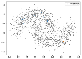
(a) Two Moons with only a few samples labeled

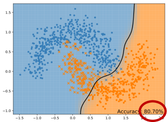
(b) Performance degraded $\approx 15\%$.

Figure 12: Illustration of initial label issue with SUMs

3.5 Potential Issues with Label Error Remediation in Practice

A potential issue may arise within the SUMER framework, which we refer to as the model coupling problem. To assist in the understanding of the model coupling problem, consider that some label correction techniques (see Sec. 4.2.1) estimate class-conditional noise rates to determine remediation: $P(\hat{Y}|Y)$. This is the probability of guessing the wrong class, $\hat{Y}$̂,whentheactualclassis$Y$.Ifthisisnear-zero,thennonoisewasdetectedandthusnoremediationwilloccur.ThismanifestswhenlabelsinferredbylabelcorrectionareindistinguishablefromSUMpredictions(i.e.,themodelsarecoupled).Noticethatthereisnodependenceonthefeaturevector$X$.\par Forreference,apredictionmodelcalculates$P(Y—X)$,whichistheprobabilityofpredictingclass$Y$givenfeaturevector$X$.Finally,consideraSUMwhosebehaviorisdescribedby$P(^Y—Y,X)$.Thisissimilartowhatalabelcorrectiontechniqueestimatesexceptthereisadependenceonthefeatures.WhenaSUMgeneratesanincorrectprediction,whichisalsousedasalabelforretraining,itisclearthattheincorrectlabelisdependentonthefeaturesbecauseafeaturevectorwasusedtogeneratetheprediction.Thisscenariocorrespondstoasmallemergingfieldinmachinelearningknownasfeature-dependentlabelnoise\cite[cite]{[\@@bibref{}{Scott19}{}{}]}.Thus,modelcouplingcanbedescribedasadisconnectbetweenthelabelcorrectionstrategy,whichassumesfeatureindependence,andaSUM,whichisdependentonthefeatures.Possiblesolutionsaretocreateanindependent,auxiliarylabelcorrectionmodel;optimizelossthatisimmunetonoise;andusedifferentviewsofthedataifpossible.Thelastpotentialsolutionissimilartotherequirementforco-trainingtohavedifferentviewsofthedata.\par$

4 Related Work

In this section, we briefly describe some of the open academic research that aligns with the framework defined by our research. Additionally, this section is meant to provide references to other potential algorithms and techniques that may be worth exploring in the future. However, please note that this list of related work is not meant to be exhaustive.

At a high-level, the work presented here for SUMER fills a particular niche that is only partially addressed in the open literature. Specifically, many of the individual components are addressed in isolation, but none of the current works put it all together in an iterative fashion and take into account issues that arise from multiple iterations of applying the various techniques or biases that arise when using self-predicted labels. Most of the work presented here focuses solely on self-updating models or error and noise remediation, for which we present related works in Secs. 4.1 and 4.2, respectively. Other key areas include: 1) uncertainty/trust in the model outputs such as active learning [1] that encompasses strategies for querying a human in the loop to obtain additional labels, output calibration [16] that seeks to improve model confidence, and uncertainty quantification in machine learning [17]; 2) understanding the data [18]; 3) concept drift [2]; 4) and online learning [19]. While substantial, this work only scratches the surface of the possible avenues to explore. Future work will build upon this initial study and incorporate additional avenues for research.

4.1 Self-updating Models and Semi-supervised Learning

In general, self-updating models fall under the semi-supervised learning paradigm in machine learning. Semi-supervised learning refers to techniques that have a set of data points that are labeled and usually with a significantly larger number of data points without labels. For SUMER, we expand on this notion and assume that there exists a set of labeled training data points to build a machine learning model that will be deployed in a dynamic environment where it will be exposed to large amounts of data that may not be represented in the initial labeled training set. Thus, self-updating will allow the model to adapt to a richer set of data than what was available in training. In semi-supervised learning, many algorithms attempt to assign labels to the unlabeled data points and then use the newly labeled data to improve the training.

Most approaches differ in calculating the relationship between the data points including: 1) clustering, 2) self-training, 3) multi-view learning, and 4) self-ensembling. Probabilistically, the methods attempt to infer the probability $P(y|\mathbf{x})$ of a class $y$ given a data point ($\mathbf{x}$). Early works clustered data points [20] [21], examining how the unlabeled data affects the shape and size of the clusters and using Baye’s theorem to approximate $P(y|\mathbf{x})$: $P(y|\mathbf{x})\propto P(\mathbf{x}|y)P(y)$. Later work estimated $P(y|\mathbf{x})$ directly using the predicted labels from models trained on the labeled training set. Each of the following subsections will give an example of a few algorithms.

4.1.1 Cluster-based approaches

Clustering-based approaches make the assumption that “close” data points tend to have the same label. Label propagation [22] is an algorithm that iteratively adds nearest unlabeled data points to the set of labeled data. In a two-label class problem (0 or 1), initially all unlabeled data points are assigned 0.5 representing uncertainty in whether that data point belongs to the 0 class or the 1 class. Until node values converge, the node values are propagated to their connected nodes representing the unlabeled data points and are averaged. Labels are then assigned based on the final value: if the value is greater than 0.5, then the data point is assigned a 1; otherwise, it is assigned a 0.

4.1.2 Self-training

Self-training uses a model’s own predictions as the labels for retraining [23]. A model is initially trained using the available labeled data. Unlabeled data is then passed through the model and assigned the label that the model predicts. Generally, labels are only provided to data points where the model has sufficient confidence. However, calibrating a model’s confidence is not straight forward [16]. A glaring problem that SUMER attempts to address is that these methods are not able to correct prediction errors. Also, most studies only examine a single iteration and do not measure the impact of mislabeled data points on subsequent iterations of self-training.

4.1.3 Multi-view learning

Multi-view learning builds on self-training. Rather than using a single model to train and label the data, multi-view learning trains multiple models with different “views” of the data. “Views” of the data can differ based on the features, data preprocessing, and/or subsets of the data. In co-training [24], where there are two views of the data, data points with confident predictions according to exactly one of the two models is moved to the training set for the other model. In other words, one model provides the labels for data points about which the other model is uncertain. This process is repeated until there are no confident predictions from one of the classifiers.

There are several variations of multi-view training that build on co-training. One of the best known multi-view training methods is tri-training [25], which leverages three independently-trained models where each initial model is diverse. For tri-training, a data point is added to the training set of a model if the other two models agree on its label. Like with co-training, this process is repeated until there are no additional data points added to a training set.

4.1.4 Self-ensembling

Self-ensembling methods are another variation on the multi-view theme of using model diversity to increase robustness. The general idea is to use a single model under different configurations. There have been several recent advances in this area focused particularly on deep learning methods where self-training-like methods are used during the training process. For example, ladder networks [26] use unlabeled data points with the goal of making a model more robust to noise. For each unlabeled example, noise is added (perturbing the input values) and the example is assigned the label predicted by the neural network on the clean version of the example. Ladder networks are mostly used in computer vision where many forms of perturbation and data augmentation are available.

Pseudo-labeling [27] uses self-training in each training epoch in neural network training. An initial model is trained on the labeled set of training examples. The trained model is then used to predict the labels of unlabeled training data (“pseudo-labels”), which is combined with the original labeled data points and the model is retrained with the pseudo-labeled and the labeled data. This is repeated until the model converges. Temporal ensembling [28] builds on pseudo-labels by providing an exponential moving average of the predictions on the unlabeled data points as training progresses. Temporal ensembling also uses a loss function on the consistency between the network outputs when using dropout and other regularization techniques. Mean teacher [29] is an improvement of temporal ensembling that stores an exponential moving average of the model parameters (weights). There are two conceptual networks: the teacher network and the student network. Initially, the teacher network is a copy of the student network. Each network will use the same mini-batch of training data, but the teacher network will add random augmentation of noise to the inputs. The (mean) teacher maintains an exponential moving average of the student network’s parameters and provides a consistency cost between the teacher and student models. The student network is updated using classification loss. Currently, mean teacher provides state-of-the-art results for semi-supervised learning in the image domain.

4.1.5 Virtual adversarial training

The previous approaches used a supervised technique to predict a label for the unlabeled points. Virtual Adversarial Training (VAT) [30] is an alternative approach that takes into account the input data distribution irrespective of the class. The goal of VAT is to make the output distribution of the model smooth such that the model is not sensitive to small perturbations in the inputs. In other words, similar data points should have similar outputs from the model. At a high-level, VAT trains a model to make the outputs of two similar inputs as close as possible. To do so, VAT starts with in an input $x$, which it transforms by adding small perturbations in an adversarial manner (meaning that the the perturbations encourage large output differences). With the adversarial data point, the model weights are updated to minimize the difference of the output of the original data point and the perturbed version. VAT can be used with data sets that are fully-labeled, partially-labeled, or have no labels.

4.1.6 Comparison of methods

The performance of the techniques is dependent on several factors, including the initial set of labeled data points. Recent work [31] compared several semi-supervised techniques to evaluate many real-world scenarios that are not commonly addressed. Their findings suggest that temporal ensembling (referred to as $\pi$-model) and VAT perform the best as illustrated in Fig. 13. As with supervised machine learning techniques, there are several biases that are present in each of the techniques that should be considered. For example, the boundaries from pseudo-labeling produces more circular clusters of the labeled data.

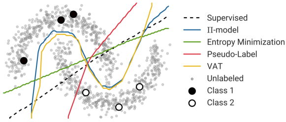
Figure 13: Comparison of multiple semi-supervised methods on the synthetic two-moons data set from Oliver et al. [31]

4.2 Label Noise Remediation

Learning with noisy labels is a machine learning problem which assumes that the labeling process (e.g., a human-in-the-loop) that provides labels for instances will occasionally miscategorize those instances (i.e., introduce errors). The goal of algorithms used to address label noise is to induce a model that performs as well as a model that was built on data with correct labels.

4.2.1 Estimating noise rates

For binary classification problems, a machine learning algorithm is essentially trying to induce a model to separate two distributions, $P_{0}$ and $P_{1}$. When label noise is present, the two distributions can be viewed as a contaminated mixture of each other [7]:

$$\tilde{P_{0}} =(1-\pi_{0})P_{0}+\pi_{0}P_{1}$$

$$\tilde{P_{1}} =(1-\pi_{1})P_{1}+\pi_{1}P_{0}$$

Many label error remediation techniques [32, 14, 7] attempt to estimate $\pi_{0}$ and $\pi_{1}$ directly from the given contaminated training samples:

$$X^{1}_{0},X^{2}_{0},\ldots,X^{n0}_{0} \sim\tilde{P_{0}}$$

$$X^{1}_{1},X^{2}_{1},\ldots,X^{n1}_{1} \sim\tilde{P_{1}}$$

Then, with access to the samples from $\tilde{P_{0}}$ and $\tilde{P_{1}}$, along with the estimated noise rates, $\pi_{0}$ and $\pi_{1}$, it should be possible to recover the true distributions, $P_{0}$ and $P_{1}$. Or, at the very least, it should be possible to induce a machine learning model as if the true distributions are known. For example, Rank Pruning [14] uses the estimated error rates to prune (i.e., remove) $\pi_{1}|\tilde{P_{1}}|$ and $\pi_{0}|\tilde{P_{0}}|$ (where $|\tilde{P_{x}}|$ represents the number of instances in class $x$), which are the least confident data points from the training set, and then reweights the remaining instances based on those noise rates.

4.2.2 Dataset augmentation

Another way to remediate errors in the labels involves altering or augmenting the training data in intelligent ways (either the instances or the labels). For example, Kegelmeyer et al. use an ensemble of anomaly detection models to create new features that have proven useful in detecting and remediating label noise [4, 33]. Resampling methods are used to increase diversity and performance in decision tree ensembles [34]. Synthetically generating data has been shown to remediate issues such as class skew [35].

Some algorithms augment the labels themselves by attempting to correct mislabeled instances. For example, Kremer et al. use ideas from active learning to select instances to relabel, based on those instances that would have the maximal impact on the model [36].

4.2.3 Specialized algorithms

Additionally, specialized algorithms can be derived to address the issue of label noise directly. For example, label spreading [12] relaxes the optimization objective used in label propagation to allow instances with provided labels to change labels, which can correct mislabeled instances. Natarajan et al. modify the loss function to address the label noise issue [6]. Their derived loss function also utilizes noise rates, but assumes that these rates are known in advance. Menon et al. proved that the balanced error rate and area under the ROC curve (AUC) are immune to label noise [37]. However, optimizing these losses might require more complex algorithms or optimization procedures.

Some algorithms are somewhat more robust to label noise, such as decision trees [38] and Random Forests [39]. The count-based methods used to determine splits and the resampling and randomness used to create the ensembles help to alleviate the effects of label noise. Additionally, there is evidence that deep learning is also quite robust to non-adversarial label noise [40].

As the main goal of SUMER is to reduce and remediate labeling errors introduced by the self-updating process, the SUMER framework involves combining techniques from self-updating / semi-supervised learning with error remediation techniques, some of which were described above. Semi-supervised learning and learning with label noise have been studied for quite a while. However, not all of the problems associated with these learning tasks have been fully solved. This section provides some potential research for future exploration.

5 Conclusion and Future Work

In this work, we have experimentally demonstrated the benefit of self-updating models (SUMs) and self-updating models with error remediation (SUMER) in both synthetic and realistic environments. In many cases, SUMs/SUMER may provide improved performance with minimal downside risk. Our conclusion is that if that environment allows, then machine learning models should be self-updated and remediated.

This work is the first step toward building a fully autonomous machine learning (AML) system. However, we have identified three main technical problems that must be solved before an end-to-end AML system can be built:

1. Identify and characterize changes in label and feature distributions in the live stream that the model is making predictions on. Another important aspect would be to identify when a new concept or concepts appear that the deployed model has not been trained to recognize. These techniques can be stand-alone or integrated into the prediction model [41].

2. Use this change information to suggest the most appropriate way to rebuild the model, e.g., incremental or full rebuild. How the model is rebuilt will differ from model-to-model. AML is largely model agnostic, but it may be necessary to devise algorithms for updating models in the appropriate way if no techniques exist for specific models of interest.

3. Augment the retraining dataset to improve the performance of the updated model. For SUMER, we validated the benefits of SUMs and label correction techniques. Future work in this area could look at weak supervision, additional label correction techniques (e.g., uncertainty quantification), and using generative models (e.g., Virtual Adversarial Training) to synthesize additional retraining data points. This is a very rich area. SUMER reduced the risk substantially, but there are still lots of potential R&D opportunities.

Future work in AML should also address the challenge of model coupling that appears when the prediction model and the label correction model provide consistent predictions, i.e., predictions that are almost always in agreement. This can be caused by both models being built using the same view of the data or the models having the same inductive bias. A view of the data refers to the feature set created during the feature engineering process. Possible solutions are to create an independent, auxiliary label correction model; optimize loss that is immune to noise; and use different views of the data if possible. The last potential solution is similar to the requirement for co-training to have different views of the data.

- [1] Settles, B., “Active learning literature survey,” Computer Sciences Technical Report 1648, University of Wisconsin–Madison (2009).
- [2] Gama, J. a., Žliobaitė, I., Bifet, A., Pechenizkiy, M., and Bouchachia, A., “A survey on concept drift adaptation,” ACM Computing Surveys 46, 44:1–44:37 (Mar. 2014).
- [3] Zhang, K., Schölkopf, B., Muandet, K., and Wang, Z., “Domain adaptation under target and conditional shift,” in [Proceedings of the 30th International Conference on Machine Learning ], Dasgupta, S. and McAllester, D., eds., Proceedings of Machine Learning Research 28, 819–827, PMLR, Atlanta, Georgia, USA (17–19 Jun 2013).
- [4] Crussell, J. and Kegelmeyer, P., “Attacking dbscan for fun and profit,” in [Proceedings of the 2015 SIAM International Conference on Data Mining ], 235–243 (2015).
- [5] Daumé, H., Kumar, A., and Saha, A., “Frustratingly easy semi-supervised domain adaptation,” in [Proceedings of the 2010 Workshop on Domain Adaptation for Natural Language Processing ], DANLP 2010, 53–59, Association for Computational Linguistics, USA (2010).
- [6] Natarajan, N., Dhillon, I. S., Ravikumar, P. K., and Tewari, A., “Learning with noisy labels,” in [Advances in Neural Information Processing Systems 26 ], Burges, C. J. C., Bottou, L., Welling, M., Ghahramani, Z., and Weinberger, K. Q., eds., 1196–1204, Curran Associates, Inc. (2013).
- [7] Scott, C., Blanchard, G., and Handy, G., “Classification with Asymmetric Label Noise: Consistency and Maximal Denoising,” in [Proceedings of the 26th Annual Conference on Learning Theory ], Shalev-Shwartz, S. and Steinwart, I., eds., Proceedings of Machine Learning Research 30, 489–511, PMLR, Princeton, NJ, USA (12–14 Jun 2013).
- [8] Raeder, T. and Chawla, N. V., “Model monitor (m2): Evaluating, comparing, and monitoring models,” J. Mach. Learn. Res. 10, 1387–1390 (Dec. 2009).
- [9] Zhu, X., “Semi-supervised learning literature survey,” Tech. Rep. 1530, Computer Sciences, University of Wisconsin-Madison (2005).
- [10] Ibañez, A., “Semi-supervised learning…the great unknown.” Think Big / Business, 30 May 2019, https://business.blogthinkbig.com/semi-supervised-learning-the-great-unknown. (Accessed: 2019).
- [11] Hammell, R., “Ships in satellite imagery.” Kaggle, 29 July 2018, https://www.kaggle.com/rhammell/ships-in-satellite-imagery. (Accessed: 4 April 2019).
- [12] Zhou, D., Bousquet, O., Lal, T. N., Weston, J., and Schölkopf, B., “Learning with local and global consistency,” in [Proceedings of the 16th International Conference on Neural Information Processing Systems ], NIPS‘03, 321–328, MIT Press, Cambridge, MA, USA (2003).
- [13] Breiman, L., “Random forests,” Machine Learning 45, 5–32 (Oct. 2001).
- [14] Northcutt, C. G., Wu, T., and Chuang, I. L., “Learning with confident examples: Rank pruning for robust classification with noisy labels,” in [Proceedings of the Thirty-Third Conference on Uncertainty in Artificial Intelligence ], UAI’17, AUAI Press (2017).
- [15] Scott, C., “A generalized Neyman-Pearson criterion for optimal domain adaptation,” Proceedings of the 30th International Conference on Algorithmic Learning Theory, vol. 98 of Proceedings of Machine Learning Research (2019).
- [16] Hyams, G., Greenfeld, D., and Bank, D., “Improved training for self-training by confidence assessments,” (2017).
- [17] Stracuzzi, D. J., Darling, M. C., Peterson, M. G., and Chen, M. G., “Quantifying uncertainty to improve decision making in machine learning,” SAND Report 2018-11166, Sandia National Laboratories (10 2018).
- [18] Smith, M. R., Martinez, T., and Giraud-Carrier, C., “An instance level analysis of data complexity,” Machine Learning 95, 225–256 (May 2014).
- [19] Saad, D., ed., [On-line Learning in Neural Networks ], Cambridge University Press, New York, NY, USA (1998).
- [20] McLachlan, G. J., “Iterative reclassification procedure for constructing an asymptotically optimal rule of allocation in discriminant analysis,” Journal of the American Statistical Association 70(350), 365–369 (1975).
- [21] Titterington, D., Smith, A., and Makov, U., [Statistical Analysis of Finite Mixture Distributions ], Wiley, New York (1985).
- [22] Zhu, X. and Ghahramani, Z., “Learning from labeled and unlabeled data with label propagation,” (2002).
- [23] Triguero, I., García, S., and Herrera, F., “Self-labeled techniques for semi-supervised learning: Taxonomy, software and empirical study,” Knowledge and Information Systems 42, 245–284 (Feb. 2015).
- [24] Blum, A. and Mitchell, T., “Combining labeled and unlabeled data with co-training,” in [Proceedings of the Eleventh Annual Conference on Computational Learning Theory ], 92–100 (1998).
- [25] Zhou, Z.-H. and Li, M., “Tri-training: Exploiting unlabeled data using three classifiers,” IEEE Transactions on Knowledge and Data Engineering 17(11), 1529–1541 (2005).
- [26] Rasmus, A., Berglund, M., Honkala, M., Valpola, H., and Raiko, T., “Semi-supervised learning with ladder networks,” in [Advances in Neural Information Processing Systems 28 ], Cortes, C., Lawrence, N. D., Lee, D. D., Sugiyama, M., and Garnett, R., eds., 3546–3554, Curran Associates, Inc. (2015).
- [27] Lee, D.-H., “Pseudo-label : The simple and efficient semi-supervised learning method for deep neural networks,” ICML 2013 Workshop : Challenges in Representation Learning (WREPL) (2013).
- [28] Laine, S. and Aila, T., “Temporal ensembling for semi-supervised learning,” (2016).
- [29] Tarvainen, A. and Valpola, H., “Mean teachers are better role models: Weight-averaged consistency targets improve semi-supervised deep learning results,” in [Advances in Neural Information Processing Systems 30 ], Guyon, I., Luxburg, U. V., Bengio, S., Wallach, H., Fergus, R., Vishwanathan, S., and Garnett, R., eds., 1195–1204, Curran Associates, Inc. (2017).
- [30] Miyato, T., Maeda, S., Koyama, M., Nakae, K., and Ishii, S., “Distributional smoothing by virtual adversarial examples,” in [4th International Conference on Learning Representations ICLR ], (2016).
- [31] Oliver, A., Odena, A., Raffel, C. A., Cubuk, E. D., and Goodfellow, I., “Realistic evaluation of deep semi-supervised learning algorithms,” in [Advances in Neural Information Processing Systems 31 ], Bengio, S., Wallach, H., Larochelle, H., Grauman, K., Cesa-Bianchi, N., and Garnett, R., eds., 3235–3246, Curran Associates, Inc. (2018).
- [32] Liu, T. and Tao, D., “Classification with noisy labels by importance reweighting,” IEEE Trans. Pattern Anal. Mach. Intell. 38, 447–461 (Mar. 2016).
- [33] Kegelmeyer, P., Shead, T. M., Crussell, J., Rodhouse, K., Robinson, D., Johnson, C., Zage, D., Davis, W., Wendt, J., Doak, J., Cayton, T., Colbaugh, R., Glass, K., Jones, B., and Shelburg, J., “Counter adversarial data analytics,” SAND Report 2015-3711, Sandia National Laboratories (2015).
- [34] Banfield, R., Hall, L., Bowyer, K., and Kegelmeyer, W., “A comparison of decision tree ensemble creation techniques,” Pattern Analysis and Machine Intelligence, IEEE Transactions on 29, 173–180 (02 2007).
- [35] Chawla, N. V., Bowyer, K. W., Hall, L. O., and Kegelmeyer, W. P., “Smote: Synthetic minority over-sampling technique,” J. Artif. Int. Res. 16, 321–357 (June 2002).
- [36] Kremer, J., Sha, F., and Igel, C., “Robust active label correction,” in [Proceedings of the Twenty-First International Conference on Artificial Intelligence and Statistics ], Storkey, A. and Perez-Cruz, F., eds., Proceedings of Machine Learning Research 84, 308–316, PMLR, Playa Blanca, Lanzarote, Canary Islands (09–11 Apr 2018).
- [37] Menon, A. K., Van Rooyen, B., Ong, C. S., and Williamson, R. C., “Learning from corrupted binary labels via class-probability estimation,” in [Proceedings of the 32nd International Conference on International Conference on Machine Learning - Volume 37 ], ICML‘15, 125–134, JMLR.org (2015).
- [38] Ghosh, A., Manwani, N., and Sastry, P. S., “On the robustness of decision tree learning under label noise,” CoRR abs/1605.06296 (2016).
- [39] Frenay, B. and Verleysen, M., “Classification in the presence of label noise: A survey,” Neural Networks and Learning Systems, IEEE Transactions on 25, 845–869 (05 2014).
- [40] Rolnick, D., Veit, A., Belongie, S. J., and Shavit, N., “Deep learning is robust to massive label noise,” CoRR abs/1705.10694 (2017).
- [41] Masud, M., Gao, J., Khan, L., Han, J., and Thuraisingham, B. M., “Classification and novel class detection in concept-drifting data streams under time constraints,” IEEE Transactions on Knowledge and Data Engineering 23(6), 859–874 (2010).