Exploiting machine learning to efficiently predict multidimensional optical spectra in complex environments

Abstract

The excited state dynamics of chromophores in complex environments determine a range of vital biological and energy capture processes. Time-resolved, multidimensional optical spectroscopies provide a key tool to investigate these processes. Although theory has the potential to decode these spectra in terms of the electronic and atomistic dynamics, the need for large numbers of excited state electronic structure calculations severely limits first principles predictions of multidimensional optical spectra for chromophores in the condensed phase. Here, we leverage the locality of chromophore excitations to develop machine learning models to predict the excited state energy gap of chromophores in complex environments for efficiently constructing linear and multidimensional optical spectra. By analyzing the performance of these models, which span a hierarchy of physical approximations, across a range of chromophore-environment interaction strengths, we provide strategies for the construction of ML models that greatly accelerate the calculation of multidimensional optical spectra from first principles.

Chromophores and their photo-dynamics play a fundamental role in controlling biological functions, ranging from photosynthesis to visual perception, and in converting solar energy into the chemical energy stored in liquid solar fuels.Scholes2011 ; Schlau-Cohen2015 ; Luk2015 ; Ashford2015 ; Brennaman2016 ; Gulati2017 ; Yadav2018 ; Son2020 These essential processes are finely tuned by the interactions between a chromophore and its complex environment. Linear and multidimensional optical spectroscopiesMukamel00 probe the electronic transitions underlying these processes, providing insights into how a chromophore’s environment tunes its energetics and optical responseEngel2007 ; Calhoun2009 ; Dostal2016 ; Dean2016 ; Duan2017 ; Maiuri2018 ; Bolzonello2018 . Theoretical models can provide a direct link between these spectroscopic observables and the underlying electronic and atomic motionsAdolphs2006 ; Muh2007 ; Olbrich2011 ; Shim2012 ; Lee2016 ; Lee2017 ; Segatta2017 ; Mallus2018 ; Blau2018 ; Jang2018 ; Loco_2018 ; Schnedermann2019 ; Segatta2019 . We have recently shown that methods based on a truncated cumulant expansion of the energy gap fluctuations provide a highly appealing approach to simulate optical spectra since they accurately capture vibronic and environmental effects for both strong and weak solvent interactionsZuehlsdorff2019 . However, the promise of using such advanced dynamics-based approaches to study linear and multidimensional optical spectroscopy is currently limited by the prohibitive cost of computing the lengthy time-sequence of electronic excitation energies required to converge the time correlation functions.

Machine learning (ML) offers the opportunity to dramatically reduce the cost of computing spectra by creating an efficient map between the chemical structure and the relevant spectroscopic propertiesMontavon2013 ; Ramakrishnan2015 ; Hase2016 ; Gastegger2017 ; Chen2018 ; Grisafi2018 ; Nebgen2018 ; Paruzzo2018 ; Pronobis2018 ; Sifain2018 ; Rodriguez2019 ; Christensen2019 ; Ghosh2019 ; Kananenka2019 ; Liu2019 ; Raimbault2019 ; Simine2019 ; Wilkins2019 ; Ye2019 ; Zhang2019 ; Li2020 ; Lu2020 ; Guan2020 ; Sommers2020 ; Kwac2020 . Here we develop and analyze the performance of three ML models for predicting electronic excitation energies of chromophores in solution, each model differing in how the environment is incorporated. By focusing on the anionic photoactive yellow protein chromophore (deprotonated $trans$-thiophenyl-$p$-coumarate, $\text{pCT}^{-}$) in water and the Nile red chromophore in both water and benzene, we demonstrate that our ML models trained on $\sim$2000 excited state electronic structure calculations can accurately capture linear and multidimensional optical spectra that would otherwise require orders of magnitude more computational effort. These ML frameworks enable the investigation of time-resolved spectroscopic simulations for a wide range of chromophore systems, creating new opportunities to connect experimental observables with electronic and atomistic dynamics.

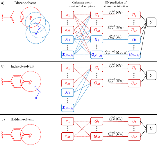
Figure 1: Schematic depictions of the (a) direct-solvent, (b) indirect-solvent, and (c) hidden-solvent approaches to incorporating a chromophore’s environment in the ML model. The dotted circles represent the cutoff distance for the local environment encoded by a given atom-centered descriptor $\bm{G}_{i}$. For visualization purposes, these depicted cutoffs are much shorter than the 5 Å cutoffs we actually employed. The connected rectangles illustrate the computational flow from chromophore and environment atomic positions and types $\{\bm{x},\bm{\mathcal{X}}\}$ to excited state energy gap prediction $U$ for the three ML models. The neural networks for a particular element type, $k_{i}$, are denoted by $f_{NN}^{(k_{i})}$ and they predict an atomic energy contribution to the energy gap $U_{i}$ given an atom-centered descriptor $\bm{G}_{i}$ for atom $i$.

Atom-centered ML approaches Behler2007 ; Bartok2010 ; Artrith2011 ; Behler2011 ; Bartok2013 ; Morawietz2016 ; Smith2017 ; Artrith2017 ; Schutt2017 ; Schutt2017a ; Yao2018 ; Zhang2018 ; Grisafi2018 ; Gastegger2018 ; Lubbers2018 ; Willatt2019 ; Unke2019 ; Artrith2019 have been used to generate spectra, such as Raman and infra-red, via evolution on a ML ground state potential energy surface Morawietz2018 ; Morawietz2019 ; Sommers2020 ; Gastegger2017 ; Nebgen2018 ; Sifain2018 ; Zhang2019 and have also been used to predict spectroscopic properties directly Gastegger2017 ; Chen2018 ; Grisafi2018 ; Nebgen2018 ; Paruzzo2018 ; Pronobis2018 ; Sifain2018 ; Christensen2019 ; Ghosh2019 ; Kananenka2019 ; Liu2019 ; Raimbault2019 ; Wilkins2019 ; Zhang2019 ; Lu2020 ; Sommers2020 ; Kwac2020 . Here we introduce an atom-centered ML approach to model the electronic energy gap $U$, the difference in energy between the ground and first excited state. As is the case for ML potentials that predict the potential energy of a system, the energy gap is given as a sum of atomic contributions, $U_{i}$, obtained from a neural network specific to the $i^{\text{th}}$ atom’s element, $f_{NN}^{(k_{i})}$, where $k_{i}$ is its element type. The input to an element specific neural network is a set of descriptors $\bm{G}_{i}$ that represent the local chemical environment around atom $i$. We employ atom-centered Chebyshev polynomial descriptors to encode the positions of nuclei around a given atomArtrith2017 in a way that incorporates translational and rotational symmetries while also being systematically improvable. Within this general ML framework we compare three different ways of including the environment and analyze the physical effects each model can and cannot capture. Figure 1 summarizes these three approaches.

The direct-solvent approach, Figure 1a, represents the most straightforward and “brute-force” application of an ML framework. In this approach, both chromophore and solvent atoms are treated equivalently in the ML model and an atomic contribution to the energy gap is calculated for each atom in the system. The total energy gap, $U$, for a system of $N$ atoms is the sum of contributions from $M$ chromophore and $N-M$ solvent atoms,

$$\begin{split}U=&\sum_{i=1}^{M}U_{i}+\sum_{j=1}^{N-M}\mathcal{U}_{j}\\ =&\sum_{i=1}^{M}f_{NN}^{(k_{i})}\left(\bm{G}_{i}(\{\bm{x},\bm{\mathcal{X}}\})\right)+\sum_{j=1}^{N-M}f_{NN}^{(\kappa_{j})}\left(\bm{\mathcal{G}}_{j}(\{\bm{x},\bm{\mathcal{X}}\})\right),\end{split}$$ (1)

where $U_{i}$ and $\mathcal{U}_{j}$ are contributions from the $i^{\text{th}}$ chromophore and $j^{\text{th}}$ solvent atoms, respectively. The position $\bm{r}_{i}$ and element type $k_{i}$ of a given chromophore atom $i$ are denoted as $\bm{x}_{i}\equiv(\bm{r}_{i},k_{i})$ and similarly for solvent atoms, $\bm{\mathcal{X}}_{j}\equiv(\bm{\mathcal{R}}_{j},\kappa_{j})$. The full set of all chromophore and solvent atom positions and element types is thus denoted $\{\bm{x},\bm{\mathcal{X}}\}$. These serve as inputs for calculating the respective chromophore, $\bm{G}_{i}$, and solvent, $\bm{\mathcal{G}}_{j}$, atom-centered descriptors.

Because chromophore excitations are often localized, not all atoms in these systems will contribute equally to the energy gap. For example, in the chromophores explored here, the changes to the electron density upon excitation are mostly localized within the $\pi$ systemZuehlsdorff2020 . Hence, other atoms not involved in the $\pi$ conjugation, including solvent atoms, are not as important in determining the excitation energy. Given enough data and a sufficiently flexible set of neural networks, a direct-solvent ML model would learn to appropriately weight the different contributions. However, owing to the large computational cost of excited state electronic structure calculations, the ideal ML model should be trainable using a minimal number of energy gaps. By explicitly incorporating simple physical approximations into the ML model, we can offload some of the physics the ML model must learn and let it focus on capturing less intuitive structure-property relationships. Consequently, these simplified and more focused ML models can be more data efficient, i.e. less data will be needed to train an accurate model. Here we leverage the locality of electronic excitations to introduce an indirect-solvent approach (Fig. 1b) where only the contributions $U_{i}$ from chromophore atoms are considered explicitly. The positions and element types of the solvent atoms $\{\bm{\mathcal{X}}\}$ still influence the energy gap, albeit indirectly through the chromophore atoms’ local environment descriptors $\bm{G}_{i}$,

$$U=\sum_{i=1}^{M}U_{i}=\sum_{i=1}^{M}f_{NN}^{(k_{i})}\left(\bm{G}_{i}(\{\bm{x},\bm{\mathcal{X}}\})\right).$$ (2)

The physical assumptions underlying the construction of this model are that solvent atoms located far from the chromophore (defined by the cutoff for the chromophore atom-centered descriptors $G_{i}$) and solvent-solvent interactions contribute negligibly to the excited state electronic energy gap. If these assumptions hold, this indirect-solvent model should be more data efficient than the direct-solvent model.

A more drastic simplification of the model would be to completely neglect solvent atom positions, as shown in the hidden-solvent model in Figure 1c. Like in the indirect-solvent model, the total energy gap in this model is simply a sum of contributions from only the chromophore atoms (Eq. 2). However, in the hidden-solvent model $\bm{G}_{i}$ is only a function of chromophore atom positions and types $\{\bm{x}\}$, i.e. $\bm{G}_{i}(\{\bm{x},\bm{\mathcal{X}}\})\to\bm{G}_{i}(\{\bm{x}\})$. By training on electronic excitation energies generated in the presence of solvent, this model can capture an average solvatochromic shift, but will be unable to connect any solvation effects on the energy gap to specific solvent configurations. Hence, this model will likely fail for systems where the chromophore interacts strongly in a site-specific manner with its environment e.g., via hydrogen bonding. On the other hand, due to its simplicity, this model should require less training data to saturate its accuracy than the other two models that encode atomistic information for the environment.

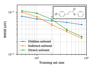
Figure 2: Learning curves for $\text{pCT}^{-}$ in water show the crossover in the RMSE validation set error for the ML solvation models as the training set size is increased. For small training sets the hidden-solvent approach gives the lowest errors whereas at larger training set size the indirect-solvent method performs best. Points represent an average over four training realizations and the bars represent the range of validation errors, the lower bar representing the minimum error and the upper bar representing the maximum error.

To assess these ML solvation models across a range of chromophore-solvent interaction strengths, we used the open source ænet packageArtrith2016 to train models for the $\text{pCT}^{-}$ chromophore in water (strong, site-specific interactions between the anionic chromophore and water), the Nile red chromophore in water (medium strength interactions), and the Nile Red chromophore in benzene (weak interactions) (SI Appendix 1). We analyze the data efficiency of the models by assessing their energy gap prediction errors as a function of training set size. We also assess how accurately the ML models reproduce the linear and multidimensional optical absorption spectra as compared to those obtained by using the energy gaps computed via the reference ab initio electronic structure method (SI Appendix 1). We compute these spectra using a cumulant expansion approach truncated at second order (SI Appendix 2), Mukamel1995 ; Mukamel1985 which we have previously shown gives accurate optical spectra in both strong and weak solvent coupling regimes Zuehlsdorff2019 . In comparatively analyzing our results, we connect the ML solvation models’ failures to their inability to capture how certain physical effects manifest in the optical spectra.

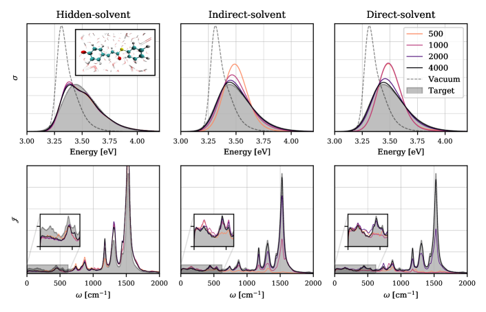
Figure 3: Linear absorption spectra (top) and spectral densities (bottom) for the three ML solvation models showing the convergence with respect to training set size ($\text{pCT}^{-}$ in water). The indirect- and direct-solvent models achieve graphical accuracy with large numbers of training points, but the hidden-solvent model never achieves this level agreement. Shading represents the target result as computed using 32,000 electronic structure energy gaps. The trained ML models were used to predict an energy gap for the same 32,000 structures and those predictions were used to compute the spectral densities and linear spectra.

The $\text{pCT}^{-}$ chromophore solvated in water is an example of an anionic chromophore that hydrogen bonds to the solvent. This serves as a particularly challenging test system since the interactions between the chromophore and solvent are sufficiently strong such that both implicit and molecular mechanics treatments of the environment fail to accurately capture the linear absorption spectrum Provorse2016 ; Isborn2012 ; Zuehlsdorff2016 ; Milanese2017 ; Zuehlsdorff2020 . Figure 2 demonstrates the compromise between the accuracy and the amount of training data for each of the ML solvation models. As the training set size increases, the root mean squared errors (RMSE) over the validation set (SI Appendix 3) for the three ML models exhibit crossovers, with the hidden-solvent method yielding the lowest error at the smallest training set size (500 training points) and the indirect-solvent model becoming the most accurate by 2000 training points with a RMSE (0.048 eV) that is considerably smaller than the standard deviation of the reference energy gaps (0.123 eV, SI Appendix 6). Both direct and indirect-solvent models are more accurate than the hidden-solvent model if at least 3000 training points are used. These crossovers can be rationalized in terms of the canonical trade-off between accuracy and variance: more complex models are more accurate when provided enough data but are prone to overfitting when using small training sets, whereas simpler models are less susceptible to overfitting but cannot capture the full physics of the system.Geman1992 Here, the direct-solvent model has the greatest complexity and can in principle incorporate the most physics while the hidden-solvent model applies a drastic simplification. Our indirect-solvent model is a compromise between these two extremes, balancing model complexity with data efficiency. This balance is reflected in the learning curve where the indirect-solvent model outperforms the other two in the range of 2000-8000 training points. Since the direct-solvent model can be trained to learn the same approximations explicitly enforced in the indirect-solvent model, we expect that with enough data and a sufficiently flexible set of neural networks it should approach and eventually surpass the accuracy of the indirect-solvent model. However, in this case, even with 8000 training points the direct-solvent model is still marginally less accurate than the indirect-solvent model.

To provide insight into how the errors in the ML-predicted energy gaps manifest in the linear optical absorption spectrum, Figure 3 shows the linear spectra (upper panels) for $\text{pCT}^{-}$ in water using training set sizes ranging from 500 to 4000 for each of the three ML models. Even when trained on the smallest dataset, all the ML models capture the spectrum significantly more accurately than if solvation effects had been completely neglected (i.e. the spectrum for the chromophore in vacuum). The direct-solvent approach converges systematically to the target result and obtains graphical agreement with the largest training set reported (4000), whereas the indirect-solvent approach converges to a similar level of accuracy with half as many training points. On the other hand, the hidden-solvent approach gives a consistent spectrum for all the training set sizes but exhibits a spurious shoulder. It is worth noting that the 500 training points needed to converge the optical spectrum for the hidden-solvent model, where only the chromophore atoms positions are fed into the network, is consistent with how many are required to converge a model for $\text{pCT}^{-}$ in vacuum (SI Appendix 5).

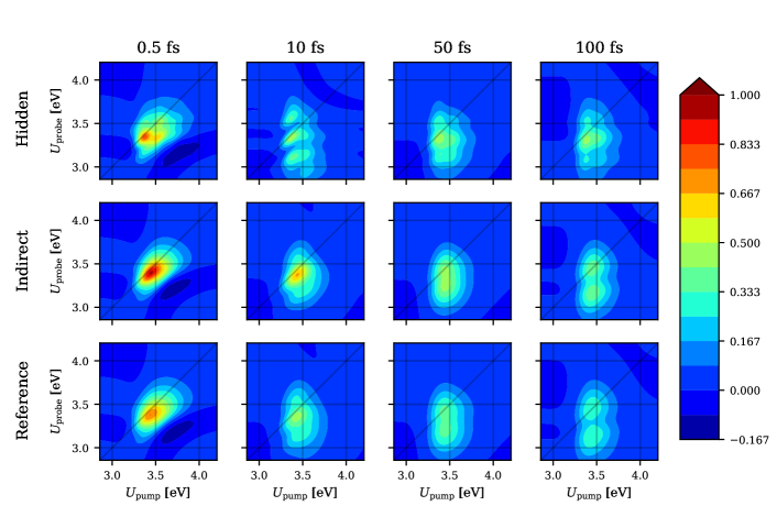
Figure 4: Two-dimensional electronic spectra (2DES) of $\text{pCT}^{-}$ in water showing the ability (inability) of the indirect-solvent (hidden-solvent) model to accurately capture spectral diffusion. A series of time delays are reported ranging from 0.5-100 fs for both the hidden-solvent (top) and indirect-solvent (middle) models, which are trained on 2000 energy gaps then used to predict the 32,000 excitation energies used to compute these spectra. The corresponding reference results (bottom) are computed using 32,000 energy gaps from electronic structure calculations.

The physical origin for these differences can be understood by examining the spectral densities in the lower panels of Figure 3, which are intimately linked to their absorption spectra via the line-shape function (SI Eq. 3). These spectral densities encode the coupling of the system’s energy gap to its vibrational modes, yielding a frequency distribution of energy gap fluctuations. The higher frequency peaks correspond to the coupling of the energy gap to intrachromophore modes while the lower frequency peaks are a result of slower solvent-coupled modesZuehlsdorff2020 . From Figure 3, we see that the hidden-solvent model, which neglects the solvent positions, systematically overpredicts the intensities of the high frequency intrachromophore modes while underestimating the lower frequency solvent modes (see inset in Figure 3). These errors manifest in the linear absorption spectrum as an over-accentuated vibronic shoulder. The ML models that explicitly include solvent positions are able to capture the intensities of both the solvent-coupled and intrachromophore modes with the indirect-solvent model needing as few as 2000 training points. Below that number, the indirect-solvent model underestimates the intensity of the high frequency modes in the spectral density, resulting in absorption spectra that are missing the high-energy vibronic tail and that are overly symmetric. For the less data efficient direct-solvent model, these same errors become apparent below 4000 training points. Despite the large discrepancies in the high frequency region of the spectral density, these errors cause small changes in the linear absorption spectrum due to the $1/\omega^{2}$ factor in SI Eq. 3. However, as we demonstrate below, these same errors manifest more prominently in the corresponding multidimensional spectra.

The photo-dynamics of chromophores are often characterized using multidimensional spectroscopy. Therefore it is important our models accurately reproduce these spectra, such as those generated from two dimensional electronic spectroscopy (2DES)Mukamel00 ; Jonas2003 ; Cho2008 . 2DES provides a more stringent and information-rich test than linear spectroscopy; at short time delays, spectra show broadened vibronic features attributable to fast intrachromophore vibrational modes and, at longer time delays, they probe the time scales of slower solvent-coupled relaxation processes. The 2DES reference spectra in Figure 4 show that after a short time delay of 0.5 fs the peak is elliptical and fairly symmetric along the diagonal since the system has not had much time to evolve. By 10 fs, the 2DES exhibits off-diagonal vibronic peaks attributable to the high-frequency vibronic modes of the chromophore. At the longest time delay (100 fs), there are two distinct peaks with the diagonal peak corresponding to ground-state bleaching and the peak below the diagonal corresponding to stimulated emission (see SI Appendix 10). Intrachromophore and solvent reorganization stabilize the excited-state and thus induce a Stokes shift in the stimulated emissionLee2017a ; Hybl2001a ; Hybl2002 . For this system, the calculated reference reorganization energy is $\lambda=0.284~{}\text{eV}$ (see SI Appendix 4) and at long time delays the stimulated emission peak will be Stokes shifted $\approx 2\lambda$ below the diagonalMukamel1995 ; Sun2016 .

Turning to the ML models, Figure 4 shows the more stringent test provided by 2DES makes the failures of the hidden-solvent model apparent; it gives a qualitatively incorrect single spectral feature at 100 fs. This failure is consistent with the hidden-solvent model’s spectral density (Fig. 3), where the intensity of the low frequency features corresponding to solvent motion are underestimated. In the corresponding 2DES, this error manifests in the enhanced vibronic structure at 10 fs and in an underestimation of the Stokes shift at 100 fs, as evinced by the failure to separate the ground state bleach and stimulated emission signals. The lack of intensity in the low frequency part of the spectral density means that less vibrational energy can be transferred from fast intrachromophore modes to collective environment modes, thus leading to a reduced Stokes shift in the limit of long delay times.

In contrast, the indirect-solvent model trained on only 2000 data points accurately captures the shapes and relative intensities of the reference 2DES. At a time delay of 100 fs, the peak separation for the indirect-solvent 2DES is 0.28 eV, which is in good agreement with the reference peak separation of 0.31 eV. In part, this good agreement reflects the accurate reproduction of the reference reorganization energy by the indirect-solvent model ($\lambda=0.262~{}\text{eV}$ vs. $\lambda=0.284~{}\text{eV}$ for the reference). When smaller training sets are used (SI Fig. 6), the accuracy of the indirect-solvent 2DES degrades. The most obvious failure is the absence of the vibronic cross-peaks at a 10 fs time delay, which is consistent with the underestimation of the high frequency intrachromophore modes in the spectral density.

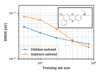
Figure 5: Learning curves for Nile red in benzene showing how the hidden-solvent model outperforms the indirect-solvent model up until 4000 training points.

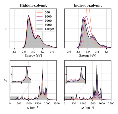
Figure 6: Linear absorption spectra (top row) and spectral densities (bottom row) for Nile red in benzene as a function of training set size using the hidden- and indirect-solvent models. Shading represents the target as computed using 30,000 electronic structure excitation energies.

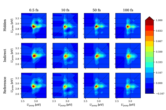
Figure 7: 2DES for Nile red in benzene at time delays of 0.5, 10, 50, and 100 fs using the hidden- and indirect-solvent models as trained on 2000 points. The reference 2DES was computed using 30,000 electronic structure excitation energies.

To address the transferability of these ML frameworks, we now consider the Nile red chromophore solvated in benzene and water representing a weakly and more strongly interacting chromophore-solvent system, respectively. Given that the indirect-solvent approach outperformed the direct method for all training set sizes in the case of $\text{pCT}^{-}$ in water, we now focus primarily on the indirect-solvent approach and how its results compare with those of the hidden-solvent approach, particularly in the case of weaker chromophore-solvent coupling.

The learning curves for Nile red in benzene in Figure 5 demonstrate that the hidden-solvent approach outperforms the indirect-solvent approach for a larger range of training set sizes when the chromophore and solvent are more weakly coupled. The RMSE of the hidden-solvent model for Nile red in benzene using 500 training points is lower than that obtained using 8000 points for $\text{pCT}^{-}$ in water and gives good agreement with the linear optical spectrum (Fig. 6). Because of the strong performance of the hidden-solvent approach, it takes 4000 training points before the indirect-solvent approach can match its accuracy. Similarly, the 2DES demonstrates that the predictions from the hidden-solvent model trained on only 2000 points reproduce the time evolution of the vibronic spectral features (Fig. 7). In contrast, the indirect-solvent model requires 4000 training points to generate 2DES of similar accuracies (SI Fig. 7). These results indicate that the interaction between Nile red and benzene is sufficiently weak such that explicit incorporation of solvent atoms in the ML model is not necessary and actually hampers training by introducing unnecessary complexity.

For a system of intermediate chromophore-environment interaction strength, we consider Nile red in water. As shown in SI Figures 8 and 9, the hidden-solvent model yields optical spectra for Nile red in water that over-accentuate vibronic features regardless of how many training points are used, consistent with the results for strongly interacting $\text{pCT}^{-}$ in water. The indirect-solvent model trained on 4000 points qualitatively reproduces the 2DES spectra for Nile red in water, but for smaller numbers of training points the spectrum exhibits a loss in off-diagonal vibronic features as is most evident at the 10 fs delay time. This phenomenon results from the spectral densities where the intensities of the high-frequency intrachromophore modes are underestimated when the indirect-solvent model is trained on small datasets. When trained on 4000 points, this error in the spectral density is rectified and consequently the corresponding indirect-solvent 2DES is in good agreement with the reference. Taken all together, our results across these different systems show that it is the chromophore-environment interaction strength that determines whether the indirect-solvent model outperforms the hidden-solvent model.

Here we have demonstrated that accurate linear and multidimensional optical spectra for solvated chromophores can be efficiently calculated using ML models to predict the excited-state electronic energy gaps. We have introduced and analyzed how different solvent representations in ML models can be more data efficient and accurate depending on the strength of the chromophore-solvent coupling. For weakly coupled systems like Nile red in benzene, we were able to completely ignore solvent positions in the ML model and trained a model which gave accurate linear and 2D electronic spectra with as few as 2000 training points. For systems with stronger and more site specific chromophore-solvent interactions, like $\text{pCT}^{-}$ in water, the simplified hidden-solvent approach did not suffice. However, by accounting for solvent atoms located close to the $\text{pCT}^{-}$ chromophore, we were able to train an accurate indirect-solvent model with 2000 training points. This work therefore provides a highly efficient scheme to generate accurate multidimensional optical spectra for chromophores in condensed phase environments. For example, the 2DES of the $\text{pCT}^{-}$ chromophore with a surrounding solvent shell of 166 water molecules (527 atoms) required 32,000 energy gaps to compute. Each one of those 32,000 reference excited-state electronic structure calculations takes  8 hours on a Nvidia Tesla K80 GPU. In contrast, our ML models can predict the energy gaps for all 32,000 configurations in one minute using a 32 core CPU node. Hence, the reduction from 32,000 to 2000 calculations represents a dramatic computational savings of 240,000 GPU hours. These massive savings can be leveraged to reduce the errors in the optical spectra that arise from other sources, such as incomplete statistical sampling of the ground state surfaceZwier2007 ; Loco2019 , the quantum dynamics approach, or in the level of electronic structure used to compute the energy gapsIsborn2013 , all of which can introduce larger errors than those in our ML model trained with only 500 points.

Finally, although we focused solely on predicting excited state energy gaps for solvated chromophores, the ML frameworks we present are generally applicable to any scalar structure-based property where a natural separation exists between a molecule and its surroundings. We also note that the labeling of the atoms belonging to the molecular center of interest and the atoms belonging to the environment is flexible. For instance, if one has pre-existing knowledge of where the electronic excitation is localized on the molecule (e.g. only the $\pi$ system) then the data efficiency of the indirect-solvent model could be improved by leveraging that intuition and further localizing the model to those specific parts of the chromophore. Similarly, if certain atoms in the environment couple strongly to the electronic excitation, they can be included with the atoms in the ML model that directly contribute to the excitation energy.

In conclusion, we have shown that ML models can accurately predict excited state properties of chromophores in complex environments, leading to dramatically reduced computational cost for simulating nonlinear optical spectra. This ability will enable the combination of ML with advanced semiclassical and quantum dynamical methods to study the photo-dynamics and multidimensional spectroscopy of chromophores in complex environments. This work therefore provides a physically informed and data efficient ML-based route to alleviate the computational bottleneck in the calculation of linear and multidimensional optical spectroscopies for a wide range of chemical systems.

Author Contributions

All authors contributed to the design of this research. M.S.C, T.J.Z., and T.M. performed the research. All authors were involved in the analysis of results and writing of the manuscript.

References

- (1) Scholes, G. D., Fleming, G. R., Olaya-Castro, A. & van Grondelle, R. Lessons from nature about solar light harvesting. Nat. Chem. 3, 763–774 (2011).
- (2) Schlau-Cohen, G. S. Principles of light harvesting from single photosynthetic complexes. Interface Focus 5, 20140088 (2015).
- (3) Luk, H. L., Melaccio, F., Rinaldi, S., Gozem, S. & Olivucci, M. Molecular bases for the selection of the chromophore of animal rhodopsins. Proc. Natl. Acad. Sci. U.S.A. 112, 15297–15302 (2015).
- (4) Ashford, D. L. et al. Molecular chromophore-catalyst assemblies for solar fuel applications. Chem. Rev. 115, 13006–13049 (2015).
- (5) Brennaman, M. K. et al. Finding the way to solar fuels with dye-sensitized photoelectrosynthesis cells. J. Am. Chem. Soc. 138, 13085–13102 (2016).
- (6) Gulati, S. et al. Photocyclic behavior of rhodopsin induced by an atypical isomerization mechanism. Proc. Natl. Acad. Sci. U.S.A. 114, E2608–E2615 (2017).
- (7) Yadav, R. K. et al. Highly improved solar energy harvesting for fuel production from co2 by a newly designed graphene film photocatalyst. Sci. Rep. 8, 16741 (2018).
- (8) Son, M., Pinnola, A., Gordon, S. C., Bassi, R. & Schlau-Cohen, G. S. Observation of dissipative chlorophyll-to-carotenoid energy transfer in light-harvesting complex ii in membrane nanodiscs. Nat. Commun. 11, 1295 (2020).
- (9) Mukamel, S. Multidimensional femtosecond correlation spectroscopies of electronic and vibrational excitations. Ann. Rev. Phys. Chem. 51, 691–729 (2000).
- (10) Engel, G. S. et al. Evidence for wavelike energy transfer through quantum coherence in photosynthetic systems. Nature 446, 782–786 (2007).
- (11) Calhoun, T. R. et al. Quantum coherence enabled determination of the energy landscape in light-harvesting complex ii. J. Phys. Chem. B 113, 16291–16295 (2009).
- (12) Dostál, J., Pšenčík, J. & Zigmantas, J. In situ mapping of the energy flow through the entire photosynthetic apparatus. Nat. Chem. 8, 705–710 (2016).
- (13) Dean, J. C., Oblinsky, D. G., Rafiq, S. & Scholes, G. D. Methylene blue exciton states steer nonradiative relaxation: Ultrafast spectroscopy of methylene blue dimer. J. Phys. Chem. B 120, 440–454 (2016).
- (14) Duan, H.-G. et al. Primary charge separation in the photosystem ii reaction center revealed by a global analysis of the two-dimensional electronic spectra. Sci. Rep. 7, 12347 (2017).
- (15) Maiuri, M., Ostroumov, E. E., Saer, R. G., Blankenship, R. E. & Scholes, G. D. Coherent wavepackets in the fenna–matthews–olson complex are robust to excitonic-structure perturbations caused by mutagenesis. Nat. Chem. 10, 177–183 (2018).
- (16) Bolzonello, L. et al. Two-dimensional electronic spectroscopy reveals dynamics and mechanisms of solvent-driven inertial relaxation in polar bodipy dyes. J. Phys. Chem. Lett. 9, 1079–1085 (2018).
- (17) Adolphs, J. & Renger, T. How Proteins Trigger Excitation Energy Transfer in the FMO Complex of Green Sulfur Bacteria. Biophys. J. 91, 2778–2797 (2006).
- (18) Müh, F. et al. -Helices direct excitation energy flow in the Fenna-Matthews-Olson protein. Proc. Natl. Acad. Sci. 104, 16862–16867 (2007).
- (19) Olbrich, C., Strümpfer, J., Schulten, K. & Kleinekathöfer, U. Theory and Simulation of the Environmental Effects on FMO Electronic Transitions. J. Phys. Chem. Lett. 14, 1771–1776 (2011).
- (20) Shim, S., Rebentrost, P., Valleau, S. & Aspuru-Guzik, A. Atomistic Study of the Long-Lived Quantum Coherences in the Fenna-Matthews-Olson Complex. Biophys. J. 102, 649–660 (2012).
- (21) Lee, M. K. & Coker, D. F. Modeling electronic-nuclear interactions for excitation energy transfer processes in light-harvesting complexes. J. Phys. Chem. Lett. 7, 3171–3178 (2016).
- (22) Lee, M. K., Bravaya, K. B. & Coker, D. F. First-Principles Models for Biological Light-Harvesting: Phycobiliprotein Complexes from Cryptophyte Algae. J. Am. Chem. Soc. 139, 7803–1814 (2017).
- (23) Segatta, F. et al. A quantum chemical interpretation of two-dimensional electronic spectroscopy of light-harvesting complexes. J. Am. Chem. Soc. 139, 7558–7567 (2017).
- (24) Mallus, M. I., Shakya, Y., Prajapati, J. D. & Kleinekathöfer, U. Environmental effects on the dynamics in the light-harvesting complexes LH2 and LH3 based on molecular simulations. Chem. Phys. 515, 141–151 (2018).
- (25) Blau, S. M., Bennett, I. G., Kreisbeck, C., Scholes, G. D. & Aspuru-Guzik, A. Local protein solvation drives direct down-conversion in phycobiliprotein PC645 via incoherent vibronic transport. Proc. Natl. Acad. Sci. 115, E3342–E3350 (2018).
- (26) Jang, S. J. & Mennucci, B. Delocalized excitons in natural light-harvesting complexes. Rev. Mod. Phys. 90, 035003 (2018).
- (27) Loco, D., Jurinovich, S., Cupellini, L., Menger, M. F. S. J. & Mennucci, B. The modeling of the absorption lineshape for embedded molecules through a polarizable QM/MM approach. Photochem. Photobiol. Sci. 17, 552–560 (2018).
- (28) Schnedermann, C. et al. A molecular movie of ultrafast singlet fission. Nat. Commun. 10, 4207 (2019).
- (29) Segatta, F., Cupellini, L., Garavelli, M. & Mennucci, B. Quantum Chemical Modeling of the Photoinduced Activity of Multichromophoric Biosystems. Chem. Rev. 119, 9361–9380 (2019).
- (30) Zuehlsdorff, T. J., Montoya-Castillo, A., Napoli, J. A., Markland, T. E. & Isborn, C. M. Optical spectra in the condensed phase: Capturing anharmonic and vibronic features using dynamic and static approaches. J. Chem. Phys. 151, 074111 (2019).
- (31) Montavon, G. et al. Machine learning of molecular electronic properties in chemical compound space. New J. Phys. 15, 095003 (2013).
- (32) Ramakrishnan, R., Hartmann, M., Tapavicza, E. & von Lilienfeld, O. A. Electronic spectra from TDDFT and machine learning in chemical space. J. Chem. Phys. 143, 084111 (2015).
- (33) Häse, F., Valleau, S., Pyzer-Knapp, E. & Aspuru-Guzik, A. Machine learning exciton dynamics. Chem. Sci. 7, 5139–5147 (2016).
- (34) Gastegger, M., Behler, J. & Marquetand, P. Machine learning molecular dynamics for the simulation of infrared spectra. Chem. Sci. 8, 6924–6935 (2017).
- (35) Chen, W. K., Liu, X. Y., Fang, W. H., Dral, P. O. & Cui, G. Deep Learning for Nonadiabatic Excited-State Dynamics. J. Phys. Chem. Lett. 9, 6702–6708 (2018).
- (36) Grisafi, A., Wilkins, D. M., Csányi, G. & Ceriotti, M. Symmetry-Adapted Machine Learning for Tensorial Properties of Atomistic Systems. Phys. Rev. Lett. 120, 36002 (2018).
- (37) Nebgen, B. et al. Transferable Dynamic Molecular Charge Assignment Using Deep Neural Networks. J. Chem. Theory Comput. 14, 4687–4698 (2018).
- (38) Paruzzo, F. M. et al. Chemical shifts in molecular solids by machine learning. Nat. Commun. 9, 4501 (2018).
- (39) Pronobis, W., Schütt, K. T., Tkatchenko, A. & Müller, K. R. Capturing intensive and extensive DFT/TDDFT molecular properties with machine learning. Eur. Phys. J. B 91, 178–184 (2018).
- (40) Sifain, A. E. et al. Discovering a Transferable Charge Assignment Model Using Machine Learning. J. Phys. Chem. Lett 9, 4495–4501 (2018).
- (41) Rodríguez, M. & Kramer, T. Machine learning of two-dimensional spectroscopic data. Chem. Phys. 520, 52–60 (2019).
- (42) Christensen, A. S., Faber, F. A. & Von Lilienfeld, O. A. Operators in quantum machine learning: Response properties in chemical space. J. Chem. Phys 150, 064105 (2019).
- (43) Ghosh, K. et al. Deep Learning Spectroscopy: Neural Networks for Molecular Excitation Spectra. Adv. Sci. 6, 1801367–1801374 (2019).
- (44) Kananenka, A. A., Yao, K., Corcelli, S. A. & Skinner, J. L. Machine Learning for Vibrational Spectroscopic Maps. J. Chem. Theory Comput. 15, 6850–6858 (2019).
- (45) Liu, S. et al. Multiresolution 3D-DenseNet for Chemical Shift Prediction in NMR Crystallography. J. Phys. Chem. Lett. 10, 4558–4565 (2019).
- (46) Raimbault, N., Grisafi, A., Ceriotti, M. & Rossi, M. Using Gaussian process regression to simulate the vibrational Raman spectra of molecular crystals. New J. Phys. 21, 105001 (2019).
- (47) Simine, L., Allen, T. C. & Rossky, P. J. Prediction of optical spectra of coarse-grained polymers as a sequence generation problem : the Recurrent Neural Networks solution. Preprint at https://arxiv.org/abs/1906.11434 (2019).
- (48) Wilkins, D. M. et al. Accurate molecular polarizabilities with coupled cluster theory and machine learning. Proc. Natl. Acad. Sci. U.S.A. 116, 3401–3406 (2019).
- (49) Ye, S. et al. A neural network protocol for electronic excitations of N-methylacetamide. Proc. Natl. Acad. Sci. U.S.A. 116, 11612–11617 (2019).
- (50) Zhang, L. et al. Deep neural network for the dielectric response of insulators. Preprint at https://arxiv.org/abs/1906.11434 (2019).
- (51) Li, J., Bennett, K. C., Liu, Y., Martin, M. V. & Head-Gordon, T. Accurate prediction of chemical shifts for aqueous protein structure on ”real World” data. Chem. Sci. 11, 3180–3191 (2020).
- (52) Lu, C. et al. Deep Learning for Optoelectronic Properties of Organic Semiconductors. J. Phys. Chem. C 124, 7048–7060 (2020).
- (53) Guan, Y., Guo, H. & Yarkony, D. R. Extending the Representation of Multistate Coupled Potential Energy Surfaces to Include Properties Operators Using Neural Networks: Application to the 1,21A States of Ammonia. J. Chem. Theory Comput. 16, 302–313 (2020).
- (54) Sommers, G., Calegari, M., Zhang, L., Wang, H. & Car, R. Raman spectrum and polarizability of liquid water from deep neural networks. Phys. Chem. Chem. Phys. Accepted Manuscript at http://dx.doi.org/10.1039/D0CP01893G (2020).
- (55) Kwac, K. & Cho, M. Machine learning approach for describing vibrational solvatochromism. J. Chem. Phys. 152, 174101 (2020).
- (56) Behler, J. & Parrinello, M. Generalized neural-network representation of high-dimensional potential-energy surfaces. Phys. Rev. Lett. 98, 146401 (2007).
- (57) Bartók, A. P., Payne, M. C., Kondor, R. & Csányi, G. Gaussian approximation potentials: The accuracy of quantum mechanics, without the electrons. Phys. Rev. Lett. 104, 136403 (2010).
- (58) Artrith, N., Morawietz, T. & Behler, J. High-dimensional neural-network potentials for multicomponent systems: Applications to zinc oxide. Phys. Rev. B 83, 153101 (2011).
- (59) Behler, J. Atom-centered symmetry functions for constructing high-dimensional neural network potentials. J. Chem. Phys. 134, 074106 (2011).
- (60) Bartók, A. P., Kondor, R. & Csányi, G. On representing chemical environments. Phys. Rev. B 87, 184115 (2013).
- (61) Morawietz, T., Singraber, A., Dellago, C. & Behler, J. How van der Waals interactions determine the unique properties of water. Proc. Natl. Acad. Sci. U.S.A. 113, 8368–8373 (2016).
- (62) Smith, J. S., Isayev, O. & Roitberg, A. E. ANI-1: an extensible neural network potential with DFT accuracy at force field computational cost. Chem. Sci. 8, 3192–3203 (2017).
- (63) Artrith, N., Urban, A. & Ceder, G. Efficient and accurate machine-learning interpolation of atomic energies in compositions with many species. Phys. Rev. B 96, 014112 (2017).
- (64) Schütt, K. T., Arbabzadah, F., Chmiela, S., Müller, K. R. & Tkatchenko, A. Quantum-chemical insights from deep tensor neural networks. Nat. Commun. 8, 6–13 (2017).
- (65) Schütt, K. T. et al. SchNet: A continuous-filter convolutional neural network for modeling quantum interactions. Advances in Neural Information Processing Systems 30, 992–1002 (2017).
- (66) Yao, K., Herr, J. E., Toth, D. W., McKintyre, R. & Parkhill, J. The TensorMol-0.1 model chemistry: A neural network augmented with long-range physics. Chem. Sci. 9, 2261–2269 (2018).
- (67) Zhang, L., Han, J., Wang, H., Car, R. & Weinan, E. Deep Potential Molecular Dynamics: A Scalable Model with the Accuracy of Quantum Mechanics. Phys. Rev. Lett. 120, 143001 (2018).
- (68) Gastegger, M., Schwiedrzik, L., Bittermann, M., Berzsenyi, F. & Marquetand, P. WACSF - Weighted atom-centered symmetry functions as descriptors in machine learning potentials. J. Chem. Phys. 148, 241709 (2018).
- (69) Lubbers, N., Smith, J. S. & Barros, K. Hierarchical modeling of molecular energies using a deep neural network. J. Chem. Phys 148, 241715 (2018).
- (70) Willatt, M. J., Musil, F. & Ceriotti, M. Atom-density representations for machine learning. J. Chem. Phys. 150, 154110 (2019).
- (71) Unke, O. T. & Meuwly, M. PhysNet: A Neural Network for Predicting Energies, Forces, Dipole Moments and Partial Charges. J. Chem. Theory Comput. 15, 3678–3693 (2019).
- (72) Artrith, N. Machine learning for the modeling of interfaces in energy storage and conversion materials. J. Phys. Energy 1, 032002 (2019).
- (73) Morawietz, T. et al. The Interplay of Structure and Dynamics in the Raman Spectrum of Liquid Water over the Full Frequency and Temperature Range. J. Phys. Chem. Lett. 9, 851–857 (2018).
- (74) Morawietz, T. et al. Hiding in the crowd : Spectral signatures of overcoordinated hydrogen bond environments. J. Phys. Chem. Lett. 10, 6067–6073 (2019).
- (75) Zuehlsdorff, T. J., Hong, H., Shi, L. & Isborn, C. M. Influence of Electronic Polarization on the Spectral Density. J. Phys. Chem. B 124, 531–543 (2020).
- (76) Artrith, N. & Urban, A. An implementation of artificial neural-network potentials for atomistic materials simulations: Performance for TiO2. Comput. Mater. Sci. 114, 135–150 (2016).
- (77) Mukamel, S. Principles of Nonlinear Optical Spectroscopy (Oxford University Press, New York, 1995).
- (78) Mukamel, S. Fluorescence and absorption of large anharmonic molecules. Spectroscopy without eigenstates. J. Phys. Chem. 89, 1077–1087 (1985).
- (79) Provorse, M. R., Peev, T., Xiong, C. & Isborn, C. M. Convergence of excitation energies in mixed quantum and classical solvent: Comparison of continuum and point charge models. J. Phys. Chem. B 120, 12148–12159 (2016).
- (80) Isborn, C. M., Götz, A. W., Clark, M. A., Walker, R. C. & Martínez, T. J. Electronic absorption spectra from MM and ab initio QM/MM molecular dynamics: Environmental effects on the absorption spectrum of photoactive yellow protein. J. Chem. Theory Comput. 8, 5092–5106 (2012).
- (81) Zuehlsdorff, T. J., Haynes, P. D., Hanke, F., Payne, M. C. & Hine, N. D. Solvent Effects on Electronic Excitations of an Organic Chromophore. J. Chem. Theory Comput. 12, 1853–1861 (2016).
- (82) Milanese, J. M., Provorse, M. R., Alameda, E. & Isborn, C. M. Convergence of Computed Aqueous Absorption Spectra with Explicit Quantum Mechanical Solvent. J. Chem. Theory Comput. 13, 2159–2171 (2017).
- (83) Geman, S., Bienenstock, E. & Doursat, R. Neural Networks and the Bias/Variance Dilemma. Neural Comput. 4, 1–58 (1992).
- (84) Jonas, D. M. Two-Dimensional Femtosecond Spectroscopy. Annu. Rev. Phys. Chem. 54, 425–463 (2003).
- (85) Cho, M. Coherent Two-Dimensional Optical Spectroscopy. Chem. Phys. Lett. 108, 1331–1418 (2008).
- (86) Lee, Y. et al. Ultrafast Solvation Dynamics and Vibrational Coherences of Halogenated Boron-Dipyrromethene Derivatives Revealed through Two-Dimensional Electronic Spectroscopy. J. Am. Chem. Soc. 139, 14733–14742 (2017).
- (87) Hybl, J. D., Ferro, A. A. & Jonas, D. M. Two-dimensional Fourier transform electronic spectroscopy. J. Chem. Phys. 115, 6606–6622 (2001).
- (88) Hybl, J. D., Yu, A., Farrow, D. A. & Jonas, D. M. Polar solvation dynamics in the femtosecond evolution of two-dimensional Fourier transform spectra. J. Phys. Chem. A 106, 7651–7654 (2002).
- (89) Sun, S.-S. & Dalton, L. R. Introduction to Organic Electronic and Optoelectronic Materials and Devices (CRC Press, Boca Raton, 2016).
- (90) Zwier, M. C., Shorb, J. M. & Krueger, B. P. Hybrid molecular dynamics‐quantum mechanics simulations of solute spectral properties in the condensed phase: Evaluation of simulation parameters. J. Comput. Chem. 28, 1572–1581 (2007).
- (91) Loco, D. & Cupellini, L. Modeling the absorption lineshape of embedded systems from molecular dynamics: A tutorial review. Int. J. Quantum Chem. 119, e25726 (2019).
- (92) Isborn, C. M., Mar, B. D., Curchod, B. F., Tavernelli, I. & Martínez, T. J. The charge transfer problem in density functional theory calculations of aqueously solvated molecules. J. Phys. Chem. B 117, 12189–12201 (2013).