Analytical correspondence between shadow radius and black hole quasinormal frequencies

Abstract

We consider the equivalence of quasinormal modes and geodesic quantities recently brought back due to the black hole shadow observation by Event Horizon Telescope. Using WKB method we found an analytical relation between the real part of quasinormal frequencies at the eikonal limit and black hole shadow radius. We verify this correspondence with two black hole families in $4$ and $D$ dimensions, respectively.

I Introduction

Quasinormal modes exist as asymptotic solutions of propagating fields (perturbations) around compact objects described by general relativity or curvature based theories of gravitation. They are characterized by a pair of numbers, a frequency of oscillation of such a system together with its damping, $\omega=\omega_{r}+i\omega_{i}$, the so-called quasinormal frequencies.

In theory, they are the outcome of a spreading wave through a gravitational potential, for which outgoing waves are the proper boundary conditions in terms of the tortoise coordinate, dispersing away of the potential barrier (since nothing comes out of the horizon). In general terms these conditions are written as a plane wave field $\Psi$ in the limits of a coordinate $x$ as $\Psi\Big{|}_{x_{\pm\infty}}\rightarrow e^{\mp i\omega x}$.

The typical vibrational spectrum that emerges from such spreading is determined by two sets of features, the geometry parameters and the inner field characteristics. Related to these characteristics we evidence two useful aspects in this letter, namely, the angular momentum (or equivalent) and overtone number. Those quantities are natural numbers connected, respectively, to the angular part of the motion equation and to the label of a quantized wave solution of its radial part.

These numbers establish a very special feature in the spectrum, whenever they are high, we have fixed values of ’density $\omega$’s. To exemplify let us recall the result in Ref. Cardoso et al. (2009), $\omega=\ell\Omega_{c}-i\nu|\lambda|,$ which established the equivalence of the real and imaginary parts of $\omega/\alpha$, $\alpha\rightarrow\ell,\nu$, with the geodesic angular velocity, $\Omega_{c}$ and Lyapunov exponent, $\lambda$.

Such astonishing result dictates a family of solutions known as the photon sphere quasinormal modes, which keep a close relation to the outermost photon orbit around the black hole (proved to be unstable). These modes are obtained traditionally with the WKB method (more details in the next section).

The relation between quasinormal modes and geodesic quantities reported in Cardoso et al. (2009) were recently revived connecting it with black holes shadows as the one reported by the Event Horizon Telescope last year Akiyama et al. (2019a, b). In the same way, gravitational lensing observables may be strictly connected to the perturbed solution, viz. to those oscillations, as pointed out in Stefanov et al. (2010).

As a general feature in spherically symmetric spacetimes the photon sphere region collapses to the value of the maxima of every black hole potential no matter which field is being considered. Such a result brings new light in the shadow phenomenon and its connection to perturbations as we will further see along this work.

This letter is organized as follows, in section II we demonstrate the equivalence of quasinormal modes at the eikonal limit and black hole shadow (first conjectured in Jusufi (2020a)) following with examples of the identification in section III. We summarize our discussion in section IV.

II Circular photon orbit, shadows, and quasinormal modes via WKB

Let us begin with a sufficiently generic line element that could represent several D-dimensional black holes with spherical symmetry given by

$$ds^{2}=-fdt^{2}+\frac{dr^{2}}{f}+r^{2}d\Omega_{D-2}^{2}.$$ (1)

Here the spherical symmetry implies $f=f(r)$. Many different field motion equations as well as a linear gravitational perturbation can be expressed with a master formula written as

$$\left[\frac{\partial^{2}}{\partial x^{2}}-\frac{\partial^{2}}{\partial t^{2}}+V(r)\right]\Psi(r,t)=0$$ (2)

where $x$ is a typical tortoise radial coordinate which maps its infinities (of the physically field propagating) into the singular points of $r$ (i.e., asymptotical infinities or horizons) via $dx=f^{-1}dr$. The potential in Eq. (2) can be generically expressed as a centrifugal term plus a function of the radial coordinate. This function encodes all possible information about the geometry of the spacetime, the theory under consideration (e.g., general relativity, Gauss-Bonnet, Horndeski, etc.), and the type of propagating field. It can be written as

$$V(r)=f(r)\left(g(r)+\frac{\ell(\ell+D-3)}{r^{2}}\right)$$ (3)

for the purpose of use in WKB method. Now, for the same spacetime defined in (1), the limiting unstable photon orbit can be defined as the solution of the equation Perlick et al. (2015)

$$\frac{d}{dr}\left(\frac{r^{2}}{f(r)}\right)\Bigg{|}_{r=r_{ps}}=0$$ (4)

Such equation contemplates a multitude of black hole solutions in general relativity, e.g. solutions with mass, charge, cosmological constant (positive), and anisotropic fluids. The concept of limiting orbit not only relates to the last stable photon geodesics around the hole, but also defines the idea of cone of avoidance Chandrasekhar (1985) as the region whose angle represents a ’dark place in the sky’ seen by a ’looking-backwards-observer’ falling into the hole,

$$\tan\frac{\Theta}{2}=\sqrt{r^{2}f}\frac{d\phi}{dr}.$$ (5)

In the Schwarzschild geometry, for instance, $\tan\frac{\Theta}{2}\propto(r-r_{ps})^{-1}(r-r_{h})^{1/2}$, and at the point $r=r_{ps}$ this observer has a cone of avoidance of exactly $\pi$ (no closed stable geodesic for $r<r_{ps}$).

Related to the same limit we stress another important quantity, the shadow radius of a black hole Jusufi (2020a, b); Bisnovatyi-Kogan and Tsupko (2017); Perlick et al. (2015), defined in terms of the photon sphere unstable orbit as

$$\textgoth{S}=\frac{r}{\sqrt{f}}\Bigg{|}_{r=r_{ps}}\,,$$ (6)

which corresponds to the angular semi-diameter of the shadow around a black hole as seen by a distant observer.

The main goal of this work is to provide the missing link that establishes the correspondence of the real part of the quasinormal modes (for whatever kind of perturbations) at the eikonal limit and the inverse of the shadow radius $\textgoth{S}$ of the black hole, and present examples of it.

The quasinormal modes were studied with a multitude of methods along the last decades. For an extensive review refer to Konoplya and Zhidenko (2011). Here we employ one of these methods, the semi-analytical WKB approximation, whose application in gravitational theory was first shown in the 80’s Iyer and Will (1987); Kokkotas and Schutz (1988); Seidel and Iyer (1990). The method was nicely extended to $6^{th}$ order Konoplya (2003), and in 2017 to $13^{th}$ order Matyjasek and Opala (2017).

For the purpose of our work the $3^{rd}$ order expansion reads

$$\omega=\Bigg{\{}V+\frac{V_{4}}{8V_{2}}\left(\nu^{2}+\frac{1}{4}\right)-\left(\frac{7+60\nu^{2}}{288}\right)\frac{V_{3}^{2}}{V_{2}^{2}}+i\nu\sqrt{-2V_{2}}\left[\frac{1}{2V_{2}}\left[\frac{5V_{3}^{4}(77+188\nu^{2})}{6912V_{2}^{4}}\right.\right.$$

$$\left.\left.-\frac{V_{3}^{2}V_{4}(51+100\nu^{2})}{384V_{2}^{3}}+\frac{V_{4}^{2}(67+68\nu^{2})}{2304V_{2}^{2}}+\frac{V_{5}V_{3}(19+28\nu^{2})}{288V_{2}^{2}}+\frac{V_{6}(5+4\nu^{2})}{288V_{2}}\right]-1\right]\Bigg{\}}^{1/2}_{r=r_{0}}$$

(7)

which produces the same expansion for the first terms of the eikonal limit when compared to the $4^{th}$ to $6^{th}$ order representation. Here $V_{i}$ represents the i-th derivative of the potential $V$ and $\nu=n+\frac{1}{2}$, $n\in\mathbb{N}$, is the overtone number. The above expression for $\omega$ is to be taken at the point $r_{0}$, defined as the maximum value of the potential $V$ through

$$\frac{dV}{dr}\Bigg{|}_{r=r_{0}}=\left[\ell(\ell+D-3)\frac{d}{dr}\left(\frac{f(r)}{r^{2}}\right)+\frac{d}{dr}(f(r)g(r))\right]\Bigg{|}_{r=r_{0}}=0.$$ (8)

The latter equation renders different values of $r_{0}$ depending on the physical field, theory, and black hole (expressed through $g$), but to leading - and first sub-leading - order its solution at the eikonal limit is the very simple relation,

$$\frac{d}{dr}\left(\frac{f(r)}{r^{2}}\right)\Bigg{|}_{r=r_{0}}=0.$$ (9)

The interesting fact is that $r_{0}$ and $r_{ps}$ represent the same point, defining $G=\frac{f(r)}{r^{2}}$, those equations can be written in the form

$$\frac{d}{dr}\left(G\right)\Bigg{|}_{r=r_{0}}=0,\hskip 56.9055pt\frac{d}{dr}\left(G^{-1}\right)\Bigg{|}_{r=r_{ps}}=0.$$ (10)

As a consequence, $r_{ps}=r_{0}$, as long as $G^{-2}|_{r=r_{ps}}\neq 0$, which is the case in general.

This result states that for every spherically symmetric black hole that possesses a photon sphere, the position of the maximum of the potential of motion equations of fields corresponds to the stability threshold for the circular null geodesic around the structure.

Finally, by expanding the relation (7), we obtain at the eikonal regime,

$$\omega=\omega_{R}-i\omega_{I}\rightarrow\left[\ell\frac{\sqrt{f(r)}}{r}\Bigg{|}_{r=r_{0}}+\frac{(D-3)\sqrt{f(r)}}{2r}\Bigg{|}_{r=r_{0}}+\mathcal{O}(\ell^{-1})\right]_{R}-$$

$$i\left[\frac{\nu}{\sqrt{2}}\frac{\sqrt{f(r)}}{r}\Bigg{|}_{r=r_{0}}\sqrt{6rf^{\prime}-6f-r^{2}f^{\prime\prime}-r^{2}f^{-1}{f^{\prime}}^{2}}\Bigg{|}_{r=r_{0}}+\mathcal{O}(\ell^{-1})\right]_{I}.$$ (11)

The imaginary part of the approximation to leading order reads

$$\omega_{I}=\frac{2\nu+1}{2\sqrt{2}}\textgoth{S}^{-1}\sqrt{2f-r^{2}f^{\prime\prime}}+\mathcal{O}(\ell^{-1}),$$ (12)

in which the square root term is the second derivative of the potential at its maximum (multiplied by other constants), a harmonic oscillator related term. As for the real part, it corresponds - to leading order - exactly to the shadow radius of the black hole and to sub-leading regime to half of its value,

$$\omega_{R}=\textgoth{S}^{-1}\left(\ell+\frac{D-3}{2}+\mathcal{O}(\ell^{-1})\right).$$ (13)

As conjectured in Jusufi (2020a) and here demonstrated, the result has an interesting interpretation for the real part of the quasinormal modes at high angular momentum regime as the shadow radius observed in black holes with spherical symmetry. The identification first appeared in Jusufi (2020a) and was further investigated for rotating spacetimes in Jusufi (2020b). In what follows we will give some examples of its application in known black hole systems.

III Results

In this section we apply the identification of the real part of quasinormal modes at the eikonal limit with the radius of black hole shadow for two different families of black hole solutions, the D-dimensional Tangherlini metric and a black hole surrounded by anisotropic fluids in 4 dimensions.

III.1 D-dimensional Tangherlini black hole

The metric corresponding to D-dimensional Tangherlini black hole Tangherlini (1963) has the same form as Eq.(1), where the metric function $f(r)$ and the angular part $d\Omega_{D-2}^{2}$ are given by

$$f(r) = 1-\frac{\mu}{r^{D-3}}$$

$$d\Omega_{D-2}^{2} = \sum_{i=1}^{D-2}\left(\prod_{n=1}^{i-1}\sin^{2}\theta_{n}\right)d\theta_{i}^{2}\,.$$ (14)

The parameter $\mu$ is related to the mass $M$ of the black hole as

$$\mu=\frac{16\pi M}{(D-2)\Omega_{D-2}}\,,\hbox{ with }\;\Omega_{D-2}=\frac{2\pi^{(D-1)/2}}{\Gamma\left(\frac{D-1}{2}\right)}\,.$$ (15)

In order to find the radius of the photon sphere we will use the usual Lagrangian formalism which for null geodesics gives

$${\cal L}=\frac{1}{2}g_{\mu\nu}\dot{x}^{\mu}\dot{x}^{\nu}=0\,.$$ (16)

Finding the canonically conjugated momenta and substituting back into this Lagrangian we can decouple the angular part and obtain the radial equation for a photon geodesic in the form,

$$\dot{r}^{2}+V_{T}(r)=0\,,$$ (17)

where the potential $V_{T}(r)$ can be written as

$$V_{T}(r)=\frac{f(r)}{r^{2}}(K^{2}+L^{2})-E^{2}\,.$$ (18)

Here $E$ and $L$ are the constants of motion associated to $t$ and $\theta_{2}$ coordinates (energy and angular momentum, respectively) and $K$ is a decoupling constant Carter (1968). Notice that we set $\theta_{1}=\pi/2$ as usual.

Applying the photon sphere conditions,

$$V_{T}(r_{ps})=0\,,\quad\left.\frac{dV_{T}}{dr}\right|_{r=r_{ps}}=0\,,\quad\left.\frac{d^{2}V_{T}}{dr^{2}}\right|_{r=r_{ps}}<0\,,$$ (19)

we obtain

$$r_{ps}=\left[\frac{8\pi M(D-1)}{\Omega_{D-2}(D-2)}\right]^{\frac{1}{D-3}}\,,$$ (20)

together with a relation between the constants of motion,

$$E^{2}=\frac{(D-3)(K+L^{2})}{(D-1)r_{ps}^{2}}\,.$$ (21)

Thus, the radius of the black hole shadow becomes

$$\textgoth{S}=\frac{r_{ps}}{\sqrt{f(r_{ps})}}=\sqrt{\frac{D-1}{D-3}}\,r_{ps}\,.$$ (22)

A similar result was found in Singh and Ghosh (2018) using a different method.

For the other side of the correspondence in Eq.(13) we can consider the massive scalar perturbation potential for a Tangherlini black hole given by Zhidenko (2006)

$$V_{s}(r)=\frac{(D-2)(D-4)}{4r^{2}}f^{2}(r)+\frac{(D-2)}{2r}f^{\prime}(r)f(r)+\left[\frac{\ell(\ell+D-3)}{r^{2}}+m^{2}\right]f(r)\,,$$ (23)

where $m$ represents the mass of the scalar perturbation. We applied the 6^th order WKB method in order to obtain the quasinormal frequencies for the fundamental mode.

In Tables 1–3 we show these frequencies for different dimensions, perturbation masses, and multipole numbers. The last two lines correspond to the frequencies obtained from Eq.(13) using the shadow approach to leading and to first subleading order, i.e., $\omega_{0}=\ell/\textgoth{S}$ and $\omega_{1}=[\ell+(D-3)/2]/\textgoth{S}$, respectively, with $\textgoth{S}$ given by (22). By comparing the frequencies in these tables we see that the conjecture in Eq.(13) is fulfilled as we reach the eikonal limit. Moreover, the scalar perturbation mass does not affect the results in this same limit.

$D=4$	$\ell=10$	$\ell=10^{2}$	$\ell=10^{3}$	$\ell=10^{5}$
$m=0.0$	2.026568929	19.34186945	192.5463789	19245.10520
$m=0.3$	2.033933121	19.34264493	192.5464569	19245.10520
$m=0.6$	2.056095784	19.34497141	192.5466905	19245.10520
$m=0.9$	2.093217069	19.34884911	192.5470800	19245.10520
$\omega_{0}$	1.924500898	19.24500898	192.4500898	19245.00898
$\omega_{1}$	2.020725943	19.34123403	192.5463149	19245.10521

Table 1: Real part of quasinormal frequencies $\omega_{R}$ for different multipole numbers $\ell$ and scalar perturbation masses $m$ in $D=4$ Tangherlini black hole.

$D=5$	$\ell=10$	$\ell=10^{2}$	$\ell=10^{3}$	$\ell=10^{5}$
$m=0.0$	6.001713288	54.81646560	543.2440142	54270.63680
$m=0.3$	6.005426726	54.81687599	543.2440558	54270.63681
$m=0.6$	6.016566980	54.81810723	543.2441800	54270.63681
$m=0.9$	6.035135991	54.82015928	543.2443871	54270.63681
$\omega_{0}$	5.427009412	54.27009412	542.7009412	54270.09412
$\omega_{1}$	5.969710354	54.81279507	543.2436422	54270.63683

Table 2: Real part of quasinormal frequencies $\omega_{R}$ for different multipole numbers $\ell$ and scalar perturbation masses $m$ in $D=5$ Tangherlini black hole.

$D=10$	$\ell=10$	$\ell=10^{2}$	$\ell=10^{3}$	$\ell=10^{5}$
$m=0.0$	12.15525866	91.93763045	891.1897864	88811.03578
$m=0.3$	12.15807589	91.93801097	891.1898256	88811.03578
$m=0.6$	12.16652560	91.93915253	891.1899435	88811.03578
$m=0.9$	12.18060185	91.94105512	891.1901398	88811.03578
$\omega_{0}$	8.880792741	88.80792741	888.0792741	88807.92741
$\omega_{1}$	11.98907021	91.91620487	891.1875518	88811.03569

Table 3: Real part of quasinormal frequencies $\omega_{R}$ for different multipole numbers $\ell$ and scalar perturbation masses $m$ in $D=10$ Tangherlini black hole.

III.2 Black holes surrounded by anisotropic fluids

The line element describing the geometry of a spherically symmetric black hole surrounded by an anisotropic fluid Kiselev (2003) is the same as in Eq.(1) with

$$f(r)=1-\frac{2M}{r}+\frac{Q^{2}}{r^{2}}-\frac{c}{r^{3w_{f}+1}},$$ (24)

characterized by the black hole mass $M$, charge $Q$, the parameter $w_{f}$ obeying the equation of state $p=w_{f}\rho$ (being $p$ and $\rho$ the pressure and energy density of the fluid, respectively) of the anisotropic fluid and $c$ is a dimensional normalization constant related to the presence of surrounding fluid.

It is worthwhile to mention some special cases of the solution (24). The Schwarzschild solution is recovered in two cases, for $Q=c=0$ and for $Q=w_{f}=0$ having its mass shifted to $2M-c$. For $Q=0$ and $w_{f}=-1$ we have the Schwarzschild-(anti) de Sitter black hole with $3c$ playing the role of a cosmological constant. The charged case includes the Reissner-Nordström-de Sitter solution for $w_{f}=-1$.

For our discussion we will consider two representative cases of (24), namely, $w_{f}=-1/2$ and $w_{f}=-2/3$. For a wide range of parameters those cases admit three horizons, an inner Cauchy horizon at $r=r_{-}$, the event horizon $r=r_{+}$, and a cosmological-like horizon $r=r_{c}$. The full discussion of causal structure of such geometries is explored in Cuadros-Melgar et al. (2020).

The equation that determines the circular photon orbit, as shown in Tangherlini case, is obtained through the value $r=r_{ps}$ that turns the effective potential for the photon a maximum as expressed by conditions (19), where in this case

$$V(r)=\frac{L^{2}}{r^{2}}f(r),$$ (25)

with $L$ standing for the angular momentum of the particle. Thus, for the case under consideration here the equation for the photon orbit is given by

$$3c(1+w_{f})r_{ps}^{(1-3w_{f})}-2r_{ps}^{2}+6Mr_{ps}-4Q^{2}=0\,.$$ (26)

Notice that the solution of this equation depends crucially on the fluid nature encoded by the parameter $w_{f}$.

Following the recipe outlined in the Sec.II, we first obtain the radius of circular photon orbit $r=r_{ps}$ for a given $w_{f}$ using the equation (26) and, then, substituting back into the expression (13) together with (6) we have the real part of quasinormal frequencies $\omega_{R}$ at the eikonal limit,

$$\frac{\omega_{R}}{\left(\ell+\frac{1}{2}\right)}=\frac{1}{\textgoth{S}}=\frac{1}{r_{ps}}\sqrt{1-\frac{2M}{r_{ps}}+\frac{Q^{2}}{r_{ps}^{2}}-\frac{c}{r_{ps}^{3w_{f}+1}}}\,.$$ (27)

	$w_{f}=-1/2$		$w_{f}=-2/3$
$c/c_{max}$	$(\ell+1/2)/\omega_{R}$	$\textgoth{S}$	$(\ell+1/2)/\omega_{R}$	$\textgoth{S}$
0.1	$5.354485444$	$5.354485444$	5.271473269	5.271473269
0.3	$6.377550833$	$6.377550833$	6.063015498	6.063015499
0.5	$7.992925474$	$7.992925474$	7.288469762	7.288469762
0.7	$11.07073257$	$11.07073257$	9.580273496	9.580273495
0.9	$21.05924133$	$21.05924133$	16.94705693	16.94705693

Table 4: Comparison between $(\ell+1/2)/\omega_{R}$ and the shadow radius $\textgoth{S}$ for $\ell=10^{5}$, $M=2Q=1$, $c_{max}\approx 0.2751$ for $w_{f}=-1/2$ and $c_{max}\approx 0.1292$ for $w_{f}=-2/3$.

In Table 4 we show the dependence of $(\ell+\frac{1}{2})/\omega_{R}$ and the shadow radius $\textgoth{S}$ with the parameter $c$ in the cases $w_{f}=-1/2$ and $w_{f}=-2/3$. Notice that in the first column the parameter $c$ is normalized by $c_{max}$, which is the maximum value permitted for $c$ in order to avoid naked singularities Cuadros-Melgar et al. (2020). From those results we observe that as the parameter $c$ of the anisotropic fluid increases, the radius of the black hole shadow $\textgoth{S}$ gets bigger in comparison to the case in the absence of the fluid. This result is similar to that in the case of the Schwarzschild black hole surrounded by a homogeneous plasma acting as a dispersive medium for the light rays Bisnovatyi-Kogan and Tsupko (2017). Also, we observe that the correspondence between $(\ell+\frac{1}{2})/\omega_{R}$ and the shadow radius $\textgoth{S}$ at the eikonal limit is fulfilled in this case as well.

In Table 5 we present the behavior of $\omega_{R}$ as we increase the multipole number $\ell$ towards the eikonal limit for the case $w_{f}=-1/2$. A similar qualitative result is obtained for $w_{f}=-2/3$.

$c/c_{max}$	$\ell=10$	$\ell=10^{2}$	$\ell=10^{3}$	$\ell=10^{5}$
0.1	$1.9613129$	$18.769346$	186.85269	18676.02425
0.3	$1.6462219$	$15.758382$	156.87840	15680.07886
0.5	$1.31311184$	$12.5735616$	125.173187	12511.12629
0.7	$0.94771582$	$9.0779137$	90.373416	12511.126286
0.9	$0.49800157$	$4.7721899$	47.508828	9032.871070

Table 5: Real part of quasinormal frequencies $\omega_{R}$ as $\ell$ increases with $w_{f}=-1/2$, $M=2Q=1$, and $c_{max}\approx 0.2751$.

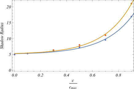
Figure 1: Shadow radius as a function of the anisotropic fluid parameter $c/c_{max}$. The upper fitting curve (orange) refers to the case $w_{f}=-1/2$ and the bottom one (blue) to $w_{f}=-2/3$. In both curves we have set $M=2Q=1$.

In Fig.(1) we show the shadow radius for several values of $c/c_{max}$ and the corresponding fitting curves for each case of interest $w_{f}=-1/2$ and $w_{f}=-2/3$. For small values of $c/c_{max}$ the shadow radius does not depend strongly on $w_{f}$. However, a different picture comes up as $c/c_{max}$ increases showing very different values depending on the fluid characteristics.

IV Discussion

In this paper we found an analytical relation between the eikonal limit of quasinormal frequencies and the black hole shadow, a result first conjectured in Jusufi (2020a). We show that every spherically symmetric black hole having an outermost photon orbit has an identification of the maxima of the potentials corresponding to perturbation fields and null geodesics.

In order to illustrate the correspondence we compute the quasinormal frequencies and shadow radius for two families of black holes, i.e., Tangherlini and a black hole surrounded by anisotropic fluids, verifying its validity.

Further investigation includes the computation of quasinormal modes in more realistic scenarios like black holes (or other astrophysical objects) with accretion disks or surrounded by plasmas.

References

References

- Cardoso et al. (2009) V. Cardoso, A. S. Miranda, E. Berti, H. Witek, and V. T. Zanchin, Phys. Rev. D 79, 064016 (2009), arXiv:0812.1806 [hep-th] .
- Cardoso et al. (2018) V. Cardoso, J. L. Costa, K. Destounis, P. Hintz, and A. Jansen, Phys. Rev. Lett. 120, 031103 (2018), arXiv:1711.10502 [gr-qc] .
- Destounis et al. (2019) K. Destounis, R. D. Fontana, F. C. Mena, and E. Papantonopoulos, JHEP 10, 280 (2019), arXiv:1908.09842 [gr-qc] .
- Destounis et al. (2020) K. Destounis, R. D. B. Fontana, and F. C. Mena, (2020), arXiv:2005.03028 [gr-qc] .
- Akiyama et al. (2019a) K. Akiyama et al. (Event Horizon Telescope), Astrophys. J. 875, L1 (2019a), arXiv:1906.11238 [astro-ph.GA] .
- Akiyama et al. (2019b) K. Akiyama et al. (Event Horizon Telescope), Astrophys. J. 875, L6 (2019b), arXiv:1906.11243 [astro-ph.GA] .
- Stefanov et al. (2010) I. Z. Stefanov, S. S. Yazadjiev, and G. G. Gyulchev, Phys. Rev. Lett. 104, 251103 (2010), arXiv:1003.1609 [gr-qc] .
- Jusufi (2020a) K. Jusufi, Phys. Rev. D 101, 084055 (2020a), arXiv:1912.13320 [gr-qc] .
- Perlick et al. (2015) V. Perlick, O. Y. Tsupko, and G. S. Bisnovatyi-Kogan, Phys. Rev. D 92, 104031 (2015), arXiv:1507.04217 [gr-qc] .
- Chandrasekhar (1985) S. Chandrasekhar, The mathematical theory of black holes (1985).
- Jusufi (2020b) K. Jusufi, (2020b), arXiv:2004.04664 [gr-qc] .
- Bisnovatyi-Kogan and Tsupko (2017) G. S. Bisnovatyi-Kogan and O. Y. Tsupko, Universe 3, 57 (2017), arXiv:1905.06615 [gr-qc] .
- Konoplya and Zhidenko (2011) R. Konoplya and A. Zhidenko, Rev. Mod. Phys. 83, 793 (2011), arXiv:1102.4014 [gr-qc] .
- Iyer and Will (1987) S. Iyer and C. M. Will, Phys. Rev. D 35, 3621 (1987).
- Kokkotas and Schutz (1988) K. Kokkotas and B. F. Schutz, Phys. Rev. D 37, 3378 (1988).
- Seidel and Iyer (1990) E. Seidel and S. Iyer, Phys. Rev. D 41, 374 (1990).
- Konoplya (2003) R. Konoplya, Phys. Rev. D 68, 024018 (2003), arXiv:gr-qc/0303052 .
- Matyjasek and Opala (2017) J. Matyjasek and M. Opala, Phys. Rev. D 96, 024011 (2017), arXiv:1704.00361 [gr-qc] .
- Tangherlini (1963) F. Tangherlini, Nuovo Cim. 27, 636 (1963).
- Carter (1968) B. Carter, Phys. Rev. 174, 1559 (1968).
- Singh and Ghosh (2018) B. P. Singh and S. G. Ghosh, Annals of Physics 395, 127–137 (2018).
- Zhidenko (2006) A. Zhidenko, Phys. Rev. D 74, 064017 (2006), arXiv:gr-qc/0607133 .
- Kiselev (2003) V. Kiselev, Class. Quant. Grav. 20, 1187 (2003), arXiv:gr-qc/0210040 .
- Cuadros-Melgar et al. (2020) B. Cuadros-Melgar, R. Fontana, and J. de Oliveira, (2020), arXiv:2003.00564 [gr-qc] .