Studying Type II supernovae as cosmological standard candles using the Dark Energy Survey

Abstract

Despite vast improvements in the measurement of the cosmological parameters, the nature of dark energy and an accurate value of the Hubble constant (H₀) in the Hubble-Lemaître law remain unknown. To break the current impasse, it is necessary to develop as many independent techniques as possible, such as the use of Type II supernovae (SNe II). The goal of this paper is to demonstrate the utility of SNe II for deriving accurate extragalactic distances, which will be an asset for the next generation of telescopes where more-distant SNe II will be discovered. More specifically, we present a sample from the Dark Energy Survey Supernova Program (DES-SN) consisting of 15 SNe II with photometric and spectroscopic information spanning a redshift range up to 0.35. Combining our DES SNe with publicly available samples, and using the standard candle method (SCM), we construct the largest available Hubble diagram with SNe II in the Hubble flow (70 SNe II) and find an observed dispersion of 0.27 mag. We demonstrate that adding a colour term to the SN II standardisation does not reduce the scatter in the Hubble diagram. Although SNe II are viable as distance indicators, this work points out important issues for improving their utility as independent extragalactic beacons: find new correlations, define a more standard subclass of SNe II, construct new SN II templates, and dedicate more observing time to high-redshift SNe II. Finally, for the first time, we perform simulations to estimate the redshift-dependent distance-modulus bias due to selection effects.

1 Introduction

Measuring accurate extragalactic distances is one of the most challenging tasks in astronomy but remains one of the best observational probes to understand the Universe’s content. Traditionally, cosmic distances are derived applying the inverse-square law to astrophysical sources with known and fixed absolute magnitudes (i.e., standard candles) or with absolute magnitudes which can be calibrated (i.e., standardisable candles). For more than two decades, Type Ia supernovae (hereafter SNe Ia; Minkowski 1941; Elias et al. 1985; Filippenko 1997; Howell 2011; Maguire 2017, and references therein) have been used as standardisable candles (e.g., Phillips 1993; Hamuy et al. 1995; Hamuy et al. 1996; Riess et al. 1996; Perlmutter et al. 1997) to measure extragalactic distances with a precision of $\sim 5$%–6% (e.g., Betoule et al. 2014; Rubin & Hayden 2016; Scolnic et al. 2018; Abbott et al. 2019). In 1998, observations of SNe Ia led to the measurement of the Universe’s expansion history and revealed the surprising accelerated growth rate of the Universe driven by an unknown effect generally attributed to dark energy (Riess et al., 1998; Schmidt et al., 1998; Perlmutter et al., 1999).

However, although SN Ia cosmology is one of the most interesting and prolific fields in astronomy, the nature of dark energy remains unknown. Furthermore, recently a new debate (e.g., Davis, 2019; Riess, 2019, and references therein) on the precise value of the Universe’s expansion rate (the Hubble constant H₀ in the Hubble-Lemaître law) appeared in the literature, with the disagreement between the local measurement from SNe Ia calibrated using Cepheid variable stars (Riess et al., 2016, 2018a, 2018b; Burns et al., 2018; Riess et al., 2019), from strong-lensing SN studies (Shajib et al., 2019) or strong-lensing quasar studies (HoLICOW; Bonvin et al. 2017) and with the high-redshift estimate from baryon acoustic oscillations (BAO; Blake & Glazebrook 2003; Seo & Eisenstein 2003) calibrated using the cosmic microwave background radiation (CMB; Fixsen et al. 1996; Jaffe et al. 2001; Spergel et al. 2007; Bennett et al. 2003; Planck Collaboration et al. 2018). The significance of this discrepancy has now increased to $>4.4\sigma$ (Riess et al., 2019), and surprisingly, this disagreement does not appear to be due to known systematic errors. Thus, further improvement to constrain H₀ and the cosmological parameters requires developing as many independent methods as possible, including gravitational wave sources (“standard sirens”; Abbott et al. 2017) or superluminous supernovae (Inserra & Smartt, 2014). With different systematic errors, those independent values will favour the local measurement or the high-redshift estimate (or perhaps some intermediate value) and will be critical to understanding the current discrepancy.

Another interesting, independent method for deriving accurate distances and measuring cosmological parameters is the use of SNe II. SNe II are characterised by the presence of strong hydrogen (H) features in their spectra (see Filippenko 1997, 2000 and Gal-Yam 2017 for overviews), and a plateau of varying steepness and length in their light curves (Barbon et al., 1979).

Despite SNe II being less luminous than SNe Ia (Richardson et al., 2014), their use as cosmic distance indicators is motivated by the facts that (1) they are more abundant than SNe Ia (Li et al., 2011; Graur et al., 2017), and (2) the physics and the nature of their progenitors are better understood. It has been proven that their progenitors are red supergiants in late-type galaxies which have retained a significant fraction of their H envelopes (e.g., Grassberg et al., 1971; Chevalier, 1976; Falk & Arnett, 1977; Van Dyk et al., 2003; Smartt et al., 2009). Unlike SNe Ia, for which no direct progenitors have been detected, SN II progenitors have been constrained, and the understanding of the explosion mechanisms of SN II has made remarkable progress in the past few decades (e.g., Woosley & Weaver, 1995; Janka, 2001; Janka et al., 2007).

In the last 20 years, after being overshadowed by the well-studied SNe Ia owing to the difficulty in getting a large sample of sufficiently high-quality data, different distance measurement methods using SNe II have been proposed and tested (e.g., Nugent & Hamuy, 2017, and references therein): the expanding photosphere method (EPM; Kirshner & Kwan 1974; Gall et al. 2018), the standard (actually standardisable) candle method (SCM; Hamuy & Pinto 2002), the photospheric magnitude method (PMM; Rodríguez et al. 2014; Rodríguez et al. 2019), and most recently the photometric colour method (PCM; de Jaeger et al. 2015, 2017b). In this paper, we focus our effort on two methods: the SCM, which is the most common and most accurate technique used to derive SN II distances, and the PCM, being the unique purely photometric method in the literature and a potential asset for the next generation of surveys such as those with the Large Synoptic Survey Telescope (LSST; Ivezić et al., 2009) and the Subaru/Hyper Suprime-Cam (HSC; Miyazaki et al., 2012; Aihara et al., 2018).

The SCM is an empirical method based on the observed correlation between SN II luminosity and photospheric expansion velocity during the plateau phase: more luminous SNe II have higher velocities (Hamuy & Pinto, 2002). This relation is physically well-understood: more luminous SNe have their hydrogen recombination front at a larger radius and thus the velocity of the photosphere is greater (Kasen & Woosley, 2009). Currently, many other studies have refined the SCM by (1) using a colour correction to perform an extinction correction (Nugent et al., 2006; Poznanski et al., 2009; Maguire et al., 2010; Olivares E. et al., 2010; D’Andrea et al., 2010; de Jaeger et al., 2015; Gall et al., 2018), (2) measuring the velocity through the absorption minimum of P-Cygni features of different lines (e.g., H$\beta$ $\lambda$4861, Fe ii $\lambda 5169$), (3) measuring the velocity using cross-correlation techniques (Poznanski et al., 2010; de Jaeger et al., 2017b), and (4) using hierarchical Gaussian processes to interpolate the magnitudes and colours at different epochs (de Jaeger et al., 2017a). All of these works have confirmed the utility of SNe II as distance indicators, constructing a Hubble diagram with a dispersion of $\sim 10$–14% in distance up to a redshift $z\approx 0.35$.

Unlike the SCM for which a spectrum is required to measure the velocity, the PCM is a purely photometric method with no input of spectral information. However, we supplement the photometric distance measurement with redshifts of the host galaxy as they are more accurate than the photometric redshifts. PCM is based on the empirical correlation between the slope of the light-curve plateau (hydrogen recombination phase) and the intrinsic brightness: more-luminous SNe II have a steeper decline (Anderson et al. 2014 and see Pejcha & Prieto 2015 for a theoretical explanation). First applied at low redshift ($z=0.01$–0.04) by de Jaeger et al. (2015), PCM was successfully extended to higher redshifts ($z<0.5$) by de Jaeger et al. (2017b).

In this paper, we use a new sample from the Dark Energy Survey (DES) Supernova Program (DES-SN) to construct the largest SN II Hubble diagram in the Hubble flow ($z>0.01$) and to assess and develop the possibility of using SNe II as distance indicators. We motivate the necessity for the SN community to dedicate specific programs for SN II cosmology – the current surveys are mostly designed for SN Ia cosmology – to improve methods and compare with SN Ia results. Future deep surveys (e.g., with LSST) and ground-based telescopes for spectroscopy such as the Keck telescopes or the next generation of 25–39 m telescopes (European Extremely Large Telescope, E-ELT, Gilmozzi & Spyromilio 2007; Giant Magellan Telescope, GMT, Johns et al. 2012; Thirty Meter Telescope, TMT, Sanders 2013) will be extremely useful for high-redshift SN II observations.

This paper is organised as follows. Section 2 contains a description of the data sample, and in Section 3 we briefly discuss the methods used to derive the Hubble diagram. We discuss our results using the SCM in Section 4, while in Section 5 those using the PCM are presented. Section 6 summarises our conclusions.

2 Data Sample

In this work, we update the Hubble diagram published by de Jaeger et al. (2017a) with SNe II from DES-SN (Bernstein et al., 2012; Brout et al., 2019a, b). For completeness, readers are reminded that the sample from de Jaeger et al. (2017a) consists of SNe II from four different surveys: the Carnegie Supernova Project-I [CSP-I;](Hamuy et al., 2006), the Sloan Digital Sky Survey-II SN Survey [SDSS-II;](Frieman et al., 2008), the Supernova Legacy Survey [SNLS;](Astier et al., 2006; Perrett et al., 2010), and the Subaru HSC Survey (Miyazaki et al., 2012; Aihara et al., 2018).

2.1 Previous sample

The previous sample used by de Jaeger et al. (2017a) consists of a total of 93 SNe II. This includes 61 from CSP-1 (58 of which have spectra) (Contreras et al., in prep.), 16 from SDSS-II (D’Andrea et al., 2010), 15 unpublished SNe II from SNLS (5 with spectroscopic information), and one from HSC (de Jaeger et al., 2017a). For more information about the different surveys and data-reduction procedures, the reader is referred to D’Andrea et al. (2010), de Jaeger et al. (2017a, b), Stritzinger et al. (2018), and references therein. Note that in this work, we update the Hubble diagram of 93 SNe II published by de Jaeger et al. (2017a), with 15 new SNe II from DES-SN (see Section 2.3).

All of the magnitudes were simultaneously corrected for Milky Way extinction ($A_{V,G}$; Schlafly & Finkbeiner 2011), redshifts due to the expansion of the Universe (K-correction; Oke & Sandage 1968; Hamuy et al. 1993; Kim et al. 1996; Nugent et al. 2002), and differences between the photometric systems (S-correction; Stritzinger et al. 2002) using the cross-filter K-corrections defined by Kim et al. (1996). For more details about these corrections, the reader is referred to Nugent et al. (2002), Hsiao et al. (2007), de Jaeger et al. (2017b), and references therein.

Finally, in this work, we use the recalibrated CSP-I photometry that will be published in a definitive CSP-I data paper by Contreras et al. (in prep.), and the explosion dates for the CSP-I sample were updated using the new values published by Gutiérrez et al. (2017).

2.2 DES-SN 5-year survey

The DES-SN was dedicated to search for astrophysical transients using the $\sim 3$ square degree Dark Energy Camera (DECam; Flaugher et al. 2015) mounted on the 4 m Blanco telescope at the Cerro Tololo Inter-American Observatory in Chile. During 5 years (2013–2018), from August to January and with a typical cadence of 4–7 nights (Diehl et al., 2016, 2018), 10 fields (see Table LABEL:tab:DES_field) were observed in the $g$, $r$, $i$, and $z$ passbands with a median limiting magnitude (respectively) of 23.7, 23.6, 23.5, and 23.3 mag for the shallow fields (C1, C2, E1, E2, S1, S2, X1, and X2) and 24.6, 24.8, 24.7, and 24.4 mag for deep fields (C3, X3). A survey overview can be found in Kessler et al. (2015), and an overview of spectroscopic targeting of the first 3 years is given by D’Andrea et al. (2018).

Table 1: Locations of the 10 DES-SN fields.

Field	$\alpha$ (J2000)	$\delta$ (J2000)
Name	$\aas@@fstack{h}$ $\aas@@fstack{m}$ $\aas@@fstack{s}$	$\circ$ $\aas@@fstack{\prime}$ $\aas@@fstack{\prime\prime}$
E1	00:31:29.9	$-$43:00:34.6
E2	00:38:00.0	$-$43:59:52.8
S1	02:51:16.8	00:00:00.0
S2	02:44:46.7	$-$00:59:18.2
C1	03:37:05.8	$-$27:06:41.8
C2	03:37:05.8	$-$29:05:18.2
C3	03:30:35.6	$-$28:06:00.0
X1	02:17:54.2	$-$04:55:46.2
X2	02:22:39.5	$-$06:24:43.6
X3	02:25:48.0	$-$04:36:00.0

The 5-year photometric data were reduced using the Difference Imaging (DIFFIMG) pipeline following the Kessler et al. (2015) prescriptions. Final photometric points were obtained via point-spread-function (PSF) photometry after host-galaxy subtraction using deep template images from each individual SN image.

Although the main science driver was to obtain high-quality light curves of thousands of SNe Ia with the goal of measuring cosmological parameters, some SN II spectroscopic follow-up observations were achieved. Spectra were obtained using the Magellan 6.5 m Clay telescope at the Las Campanas Observatory in Chile, the Anglo-Australian 3.9 m telescope situated at the Siding Spring Observatory in Australia, and the 10 m Keck-II telescope on Maunakea in Hawaii. The Anglo-Australian 3.9 m telescope spectra were obtained under the OzDES program (Yuan et al., 2015) and reduced with 2dFDR (AAO Software Team, 2015), while the other spectra were reduced following standard procedures (bias subtraction, flat-field correction, one-dimensional extraction, wavelength calibration, and flux calibration) using IRAF routines. Over 5 years, a total of 56 spectroscopically confirmed SNe II were discovered by DES-SN.

2.3 Standard Candle Method sample

Following D’Andrea et al. (2010), the final DES-5yr SN II sample adopted for the SCM was selected using five selection requirements (cuts): (1) a well-defined explosion date and a nondetection in the same observing season before the first detection of the SN, (2) photometric data up to 45 d in the rest frame after the explosion (no light-curve extrapolation), (3) at least one spectrum taken between 13 and 90 d (rest frame) to measure the H$\beta$ line velocity (see Section 3), (4) their spectra must display clear hydrogen P-Cygni profiles, and (5) the light curves should not exhibit unusual features (such as SNe IIb). In Appendix A, Table 7 provides a list of all the spectroscopically confirmed SNe II, and for each SN we indicate whether it passed the cuts. “SCM” is noted if the SN is useful for the SCM, while the SNe that failed are labeled with PHOT (no photometric data up to 45 d after the explosion), EXP (no explosion date), SPEC (no spectrum), P-Cygni (no clear P-Cygni profile), or LC (unusual light curves).

From the 56 spectroscopically confirmed SNe II, 15 passed the five cuts and are useful for our SCM analysis. One SN was rejected owing to the absence of a spectrum after 13 d, 24 lack a precise explosion date, three lack sufficient photometry (last photometric point $<45$ d), one has a slowly rising light curve typical of SNe IIb, and 12 do not exhibit clear P-Cygni profiles (generally affected by host-galaxy light). The low success rate (15/56 SNe II) is not surprising, because out of the 56 spectroscopically confirmed SNe II only 27 SNe II are potentially useful for the SCM. As the main goal of the spectroscopy was to classify the object, the majority of spectra have low signal-to-noise ratios (S/N). In the future, with a survey dedicated to SNe II and spectra of sufficient quality to measure the expansion velocities (see Section 3), the rate of useful SNe II for SCM will increase.

The final redshift distribution is presented in Figure 1. The SCM DES-SN sample has a concentration of objects with $z=0.1$–0.2 and only two SNe at high redshift ($\sim 0.35$). The gap in the range $0.2<z<0.35$ is due to our different selection cuts. If we include the 56 spectroscopically confirmed SNe II, the DES-SN distribution looks different, with nine SNe II in the range $0.2<z<0.25$ and five SNe II with $z>0.25$ (only two useful for the SCM). Eight SNe II with $z>0.2$ have been removed owing to the lack of an explosion date, one for the absence of photometric data after 40 d, and three owing to the P-Cygni profile cut.

In Figure 2 we present the DES-SN measured light curves for the 15 SNe II discovered by DES-SN and chosen for our SCM sample. Figure 3 shows all of the spectra used to measure the expansion velocities. The full set of light curves and spectra of SNe II discovered by DES-SN will be available to the community (see Appendix B and Appendix C) and be can be requested from the authors or for download.

The final SCM sample thus consists of 93 SNe II: 58 (CSP-I) $+$14 (SDSS-II) $+$5 (SNLS) $+$1 (HSC) $+$15 (DES-SN). Note that in contrast to (de Jaeger et al., 2017a), we use SN 2006iw and SN 2007ld from the CSP-I sample and not from the SDSS-II sample. Both SNe have better-sampled light curves in the new recalibrated CSP-I photometry (Contreras et al., in prep.). In Table 2, we define the different samples employed and the different cuts used in this work.

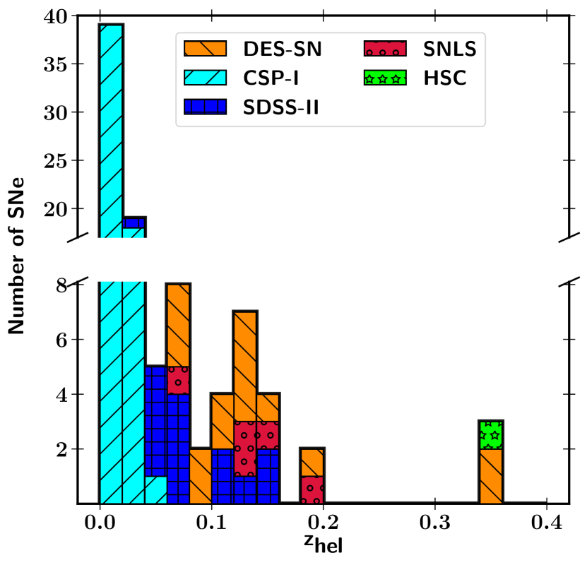
Figure 1: Histogram of the SN II sample redshift distribution. SN from CSP-I, SDSS-II, SNLS, HSC, and DES-SN are respectively displayed in cyan ($/$), blue ($+$), red ($\circ$), lime ($\star$), and orange ($\backslash$). The redshift bin size is 0.02.

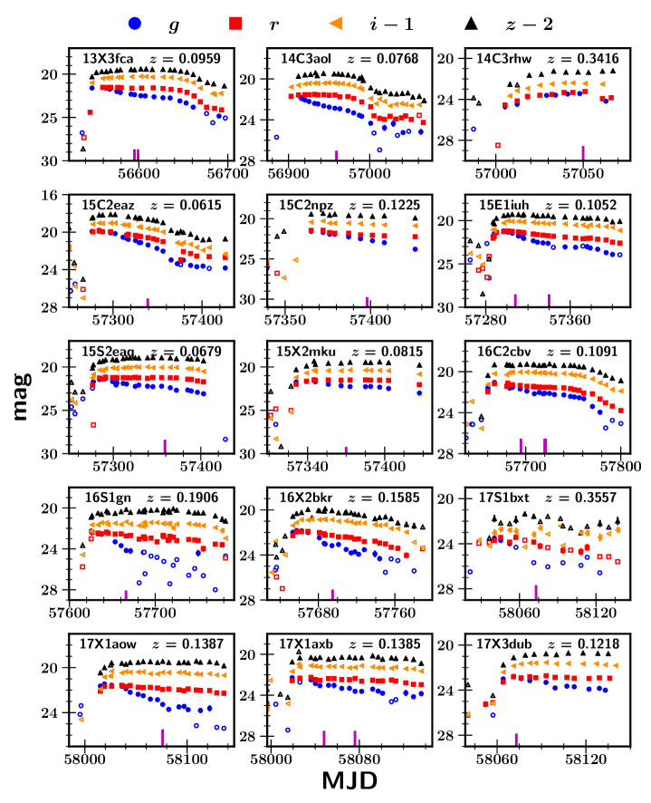
Figure 2: Observed light curves of the SNe II in our SCM sample which were discovered by DES-SN. Blue circles are magnitudes in the $g$ band, red squares are $r$, orange left triangles are $i-1$, and black top triangles are $z-2$. Empty symbols represent real points with flux/err $<3$, where “flux/err” is simply the flux divided by its uncertainty. The abscissa is the Modified Julian Date (MJD). In each panel, the IAU name and the redshift are given in the upper right. Vertical magenta lines indicate the epochs of optical spectroscopy.

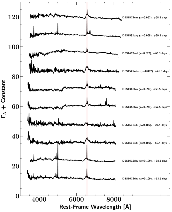
Figure 3: Spectra of the 15 SNe II from the DES-SN sample used for the SCM. The spectra are shown in the rest frame, and the date listed for each SN is the number of days since explosion (rest frame). The redshift of each SN is labelled. The spectra were binned (10 Å). The red vertical line corresponds to H$\alpha$ ($\lambda$6563) in the rest frame.

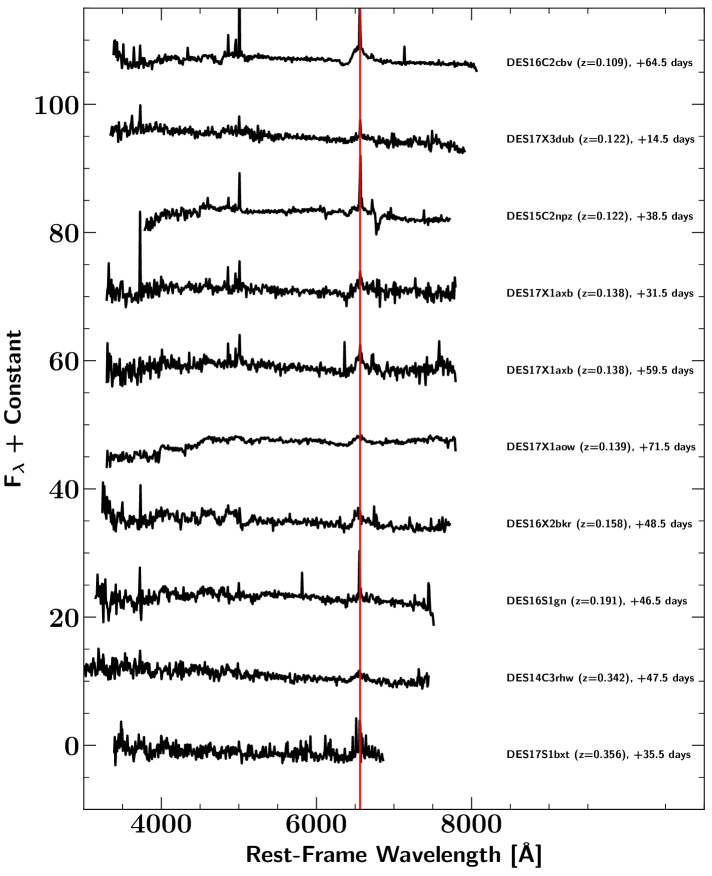
Figure 3: (Cont.) Spectra of the 15 SNe II from the DES-SN sample used for the SCM. The spectra are shown in the rest frame, and the date listed for each SN is the number of days since explosion (rest frame). The redshift of each SN is labelled. The spectra were binned (10 Å). The red vertical line corresponds to H$\alpha$ ($\lambda$6563) in the rest frame.

2.4 Photometric Colour Method sample

The sample used for the PCM includes the SCM sample plus 12 SNe II for which no clear P-Cygni profile is seen in their spectra. After light-curve inspection, we removed three SNe II: DES15X3nad, whose light curve is short and looks like that of a SN IIb, and DES17C3aye and DES17C3bei, whose $g$-band light curves exhibit a second bump perhaps caused by ejecta interacting with circumstellar matter (relatively narrow lines are present in their spectra). All of the light curves and spectra are shown in Appendix B. The final PCM sample is thus composed of 115 SNe II (61 + 14 + 15 + 1 + 24; CSP-I + SDSS-II + SNLS + HSC + DES-SN, respectively). A summary of all the SNe II available and the different cuts can be found in Table 2.

Table 2: Summary of all the SNe II available and used per survey.

Survey	All	Unique	Spectrum	Outliers	$z>0.01$	$Texp$	Photo	3$\sigma$ clipping	Used
CSP-I	61 (61)	61 (61)	58 (61)	58 (61)	44 (47)	39 (42)	37 (40)	37 (40)	37 (40)
SDSS-II	16 (16)	14 (14)	14 (14)	14 (14)	14 (14)	13 (13)	13 (13)	13 (13)	13 (13)
SNLS	15 (15)	15 (15)	5 (15)	5 (15)	5 (15)	4 (14)	4 (14)	4 (14)	4 (14)
HSC	1 (1)	1 (1)	1 (1)	1 (1)	1 (1)	1 (1)	1 (1)	1 (1)	1 (1)
DES-SN	27 (27)	27 (27)	15 (27)	15 (24)	15 (24)	15 (23)	15 (23)	15 (22)	15 (22)
Total	120 (120)	118 (118)	93 (118)	93 (115)	79 (101)	72 (93)	70 (91)	70 (90)	70 (90)

Notes: For each survey, the number of SNe II used for the SCM and the PCM (written in parentheses) is shown for different selection cuts. Unique: we removed two SNe II from SDSS-II in common with the CSP sample, spectrum: for the SCM we need at least one spectrum, outliers: from the PCM sample after light-curve inspection we removed three SNe II from the DES-SN sample, $z>0.01$: only select SNe II in the Hubble flow, $Texp$: SNe II with explosion date with an uncertainty $leq10$ d, photo: photometry data at 43 d after the explosion, and finaly, $3\sigma$ clipping: one SN II from DES-SN is identified as an outlier.

3 Methodology

In this section, we describe how the quantities (expansion velocities, magnitudes, and colours) required to derive the Hubble diagram are obtained. As the methodology is exactly the same as that used by de Jaeger et al. (2017a), only a brief description is presented here.

3.1 Photospheric velocities

The vast majority of DES-SN follow-up spectroscopy was performed to provide host-galaxy redshifts and classifications, so the average S/N of the spectra is low. A direct measurement of the H$\beta$ velocity from the minimum flux of the absorption component of the P-Cygni profile is difficult. However, Poznanski et al. (2010) and de Jaeger et al. (2017a) (at low-$z$ and at high-$z$, respectively) have demonstrated that for noisy spectra the H$\beta$ velocity can be determined by computing the cross-correlation between the observed spectra and a library of high S/N SN II spectra (templates) using the Supernova Identification code (SNID; Blondin & Tonry 2007). Velocities from direct measurement or using SNID have shown a dispersion of only 400 km s^-1, the same order of magnitude as the uncertainties (see Figure 3, de Jaeger et al. 2017a).

We cross-correlated each observed spectrum with the SN II template library spectra (for which the H$\beta$ $\lambda$4861 velocities have been measured precisely from the minimum flux of the absorption component), constraining the wavelength range to 4400–6000 Å (rest frame). For each spectrum, the resulting velocities are the sum of the template velocities (measured from the minimum flux) and the relative Doppler shift between the observed spectrum and the template. Finally, the velocities of the top 10% best-fitting templates are selected; the final velocity and its uncertainty correspond to the weighted mean and standard deviation of those selected templates. We add to the velocity error derived from the cross-correlation technique a value of 150 km s^-1, in quadrature, to account for the rotational velocity of the galaxy at the SN position (Sofue & Rubin, 2001). For example, in Figure 4 of Galbany et al. (2014), we can see that the rotational velocity of the host galaxy reaches $\sim 150$ km s^-1 with respect to the centre, measured from integral field spectroscopy of a large sample of SN Ia host galaxies. Additionally, for a SN located farther from the centre, larger differences are seen between the redshift at the SN position and the redshift of the host-galaxy nucleus. Note that all of the CMB redshifts were corrected to account for peculiar flows induced by visible structures using the model of Carrick et al. (2015).

3.2 Light-curve parameters

To derive the magnitude and the colour at different epochs, we model the light curves using hierarchical Gaussian processes (GP). This method has been successfully applied in different SN studies (Mandel et al., 2009; Mandel et al., 2011; Burns et al., 2014; Lochner et al., 2016; de Jaeger et al., 2017a; Inserra et al., 2018). To apply the GP method we use the fast and flexible Python library George developed by Ambikasaran et al. (2015). For a more quantitative comparison between the GP and linear interpolation methods, the reader is referred to de Jaeger et al. (2017a).

To measure the slope of the plateau during the recombination phase ($s_{2}$), we use a Python program which performs a least-squares fitting of the light curves corrected for Milky Way extinction and K/S-corrections. The choice between one or two slopes is achieved using the statistical method F-test. A full analysis of these slopes for our sample together with SNe from the literature will be published in a forthcoming paper.

3.3 Hubble diagram

The SCM is based on the correlation between the SN absolute magnitude and the photospheric expansion velocity and the colour. The observed magnitude can be modelled as

$$\begin{split}m^{\mathrm{model}}_{i}=&\mathcal{M}_{i}-\alpha\,\mathrm{log_{10}}\left(\frac{v_{\mathrm{H\beta}}}{<v_{\mathrm{H\beta}}>}\right)\\ +&\beta[(r-i)-<(r-i)>]+5\,\mathrm{log_{10}}(\mathcal{D}_{L}(z_{\mathrm{CMB}}|\Omega_{\mathrm{m}},\Omega_{\mathrm{\Lambda}})),\end{split}$$ (1)

where $i$ is the $i$-band filter, $(r-i)$ is the colour ($<(r-i)>\approx-0.04$ mag; the average colour), $v_{\mathrm{H\beta}}$ is the velocity measured using H$\beta$ absorption ($<v_{\mathrm{H\beta}}>$ $\sim 6000$ km s^-1; the average value), $\mathcal{D}_{L}(z_{\mathrm{CMB}}|\Omega_{\mathrm{m}},\Omega_{\mathrm{\Lambda}}$) is the luminosity distance ($\mathcal{D}_{L}$ = H${}_{0}d_{L}$) for a cosmological model depending on the cosmological parameters $\Omega_{m}$, $\Omega_{\Lambda}$, the CMB redshift $z_{\rm CMB}$, and the Hubble constant. Finally, $\alpha$, $\beta$, and $\mathcal{M}_{i}$ are free parameters, with $\mathcal{M}_{i}$ corresponding to the “Hubble-constant-free” absolute magnitude ($\mathcal{M}_{i}=M_{i}-5\,{\rm log}_{10}({\rm H}_{0})+25$).

To determine the best-fitting parameters and to derive the Hubble diagram, a Monte Carlo Markov Chain (MCMC) simulation is performed using the Python package EMCEE developed by Foreman-Mackey et al. (2013). As discussed by Poznanski et al. (2009), D’Andrea et al. (2010), and de Jaeger et al. (2017a), the minimised likelihood function is defined as

$$-2\,\mathrm{ln}(\mathcal{L})=\sum_{\mathrm{SN}}\left\{\frac{\left[m^{\mathrm{obs}}_{i}-m^{\mathrm{model}}_{i}\right]^{2}}{\sigma^{2}_{\mathrm{tot}}}+\mathrm{ln}(\sigma^{2}_{\mathrm{tot}})\right\},$$ (2)

where we sum over all SNe II available, $m_{i}^{\mathrm{obs}}$ is the observed $i$-band magnitude corrected for Milky Way extinction and K/S-corrections, and $m_{i}^{\mathrm{model}}$ is the model defined in Equation 1. The total uncertainty $\sigma_{\mathrm{tot}}$ is defined as

$$\begin{split}\sigma^{2}_{\mathrm{tot}}=&\sigma^{2}_{m_{i}}+\left(\frac{\alpha}{\mathrm{ln}10}\frac{\sigma_{v_{\mathrm{H\beta}}}}{v_{\mathrm{H\beta}}}\right)^{2}+(\beta\sigma_{(r-i)})^{2}\\ &+\left(\sigma_{z}\frac{5(1+z)}{z(1+z/2)\,\mathrm{ln}(10)}\right)^{2}+\sigma^{2}_{\mathrm{obs}}+\sigma^{2}_{\mathrm{lensing}}+\sigma^{2}_{\mathrm{lc}},\end{split}$$ (3)

where $\sigma_{m_{i}}$, $\sigma_{v_{H\beta}}$, $\sigma_{(r-i)}$, and $\sigma_{z}$ are the apparent $i$-band magnitude, velocity, colour, and redshift uncertainties. The quantity $\sigma_{\mathrm{obs}}$ includes the true scatter in the Hubble diagram and any misestimates of observational uncertainties.

Unlike the case of de Jaeger et al. (2017b), the total uncertainty $\sigma_{\mathrm{tot}}$ includes two new terms: a statistical uncertainty caused by the gravitational lensing ($\sigma_{\mathrm{lensing}}=0.055z$; Jönsson et al. 2010) and a covariance term ($\sigma_{\mathrm{lc}}$) to account for correlations between magnitude, colour, and velocity. The covariance term is a function of $\alpha$ and $\beta$; following Amanullah et al. (2010),

$$\sigma^{2}_{\mathrm{lc}}=2\alpha C_{m,{\rm vel}}-2\beta C_{m,{\rm col}}-2\alpha\beta C_{{\rm vel,col}}.$$ (4)

To derive $C_{m,{\rm vel}}$, $C_{m,{\rm col}}$, and $C_{{\rm vel,col}}$, we run 3000 simulations where for each simulated SN, the magnitude, colour, and velocity are taken at an epoch of 43 d (see Section 4.1) plus a random error (Gaussian distribution) from their uncertainties. The covariance for each SN using the 3000 magnitudes, colours, and velocities is then calculated.

For the PCM, the methodology is identical to that used for the SCM, except that instead of using a velocity correction, we use the $s_{2}$ slope correction. The observed magnitudes can be modeled as

$$m^{\mathrm{model}}_{i}= \mathcal{M}_{i}-\alpha s_{2}+\beta(r-i)+5\,\mathrm{log_{10}}(\mathcal{D}_{L}(z_{\mathrm{CMB}}|\Omega_{\mathrm{m}},\Omega_{\mathrm{\Lambda}})),$$ (5)

where all of the quantities are described above (see Eq. 1). As for the SCM, the best-fitting PCM parameters are derived using a MCMC simulation by minimising a similar likelihood function as defined in Eq. 3, except that in the total uncertainty, $\sigma_{\mathrm{tot}}$, $\left(\frac{\alpha}{\mathrm{ln}10}\frac{\sigma_{v_{\mathrm{H\beta}}}}{v_{\mathrm{H\beta}}}\right)^{2}$ is replaced by $(\alpha\sigma_{s_{2}})^{2}$.

4 SCM RESULTS

First, in Section 4.1, we assume a $\Lambda$CDM cosmological model ($\Omega_{m}=0.3$, $\Omega_{\Lambda}=0.7$) and present an updated SN II Hubble diagram using the SCM. Then, in Section 4.3, assuming a flat universe ($\Omega_{m}+\Omega_{\Lambda}=1$), we constrain the matter density ($\Omega_{m}$). Finally, we discuss differences between the samples and the effect of systematic errors on the distance modulus in Sections 4.2, 4.4, and 4.5.

4.1 Fixed cosmology: $\Omega_{m}=0.3$, $\Omega_{\Lambda}=0.7$

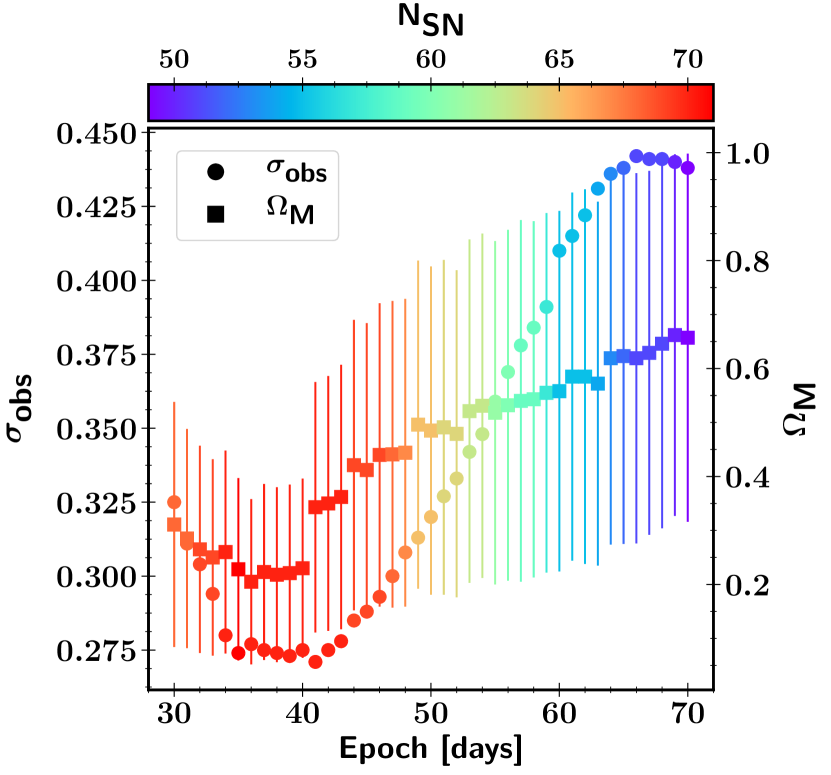
Figure 4: Variation by epoch of the intrinsic dispersion in the Hubble diagram (circles and left ordinate axis) and $\Omega_{m}$ (squares and right ordinate axis) using the SCM. The colour bar at top represents the different sample sizes. For clarity, only the $\Omega_{m}$ uncertainties are plotted.

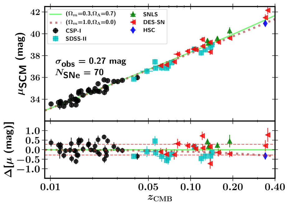
Figure 5: Hubble diagram (top) and residuals from the $\Lambda$CDM model (bottom) using the SCM as applied to the data taken from CSP-I (black circles; de Jaeger et al. 2017b), SDSS-II (cyan squares; D’Andrea et al. 2010), SNLS (green triangles; de Jaeger et al. 2017b), HSC (blue diamond; de Jaeger et al. 2017a), and DES-SN (red left triangles; this work). The lime solid line is the Hubble diagram for the $\Lambda$CDM model ($\Omega_{m}=0.3$, $\Omega_{\Lambda}=0.7$), while the brown dot line is for an Einstein-de Sitter cosmological model ($\Omega_{m}=1.0$, $\Omega_{\Lambda}=0.0$). In both models, we use H${}_{0}=70$ km s^-1 Mpc^-1 to standardise the SN II brightness. We present the number of SNe II available at this epoch ($N_{\rm SNe}$), the epoch after the explosion, and the observed dispersion ($\sigma_{\rm obs}$).

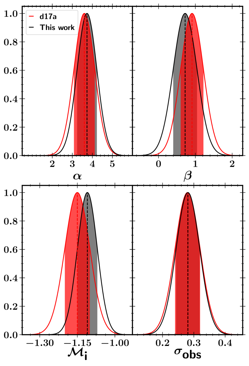
Figure 6: Comparison of the best-fitting parameters using the SCM derived by de Jaeger et al. (2017a) in red and those obtained in this work (in black) with the DES-SN sample. Top left: Distributions of $\alpha$. Top right: Distributions of $\beta$. Bottom left: Distributions of “Hubble-constant-free” absolute magnitude ($\mathcal{M}_{i}$). Bottom right: Distributions of observed dispersion ($\sigma_{\rm obs}$). In each panel, the vertical dashed line represents the average value, while the filled region represents the $1\sigma$ uncertainty.

To minimise the effect of peculiar-galaxy motions, we select SNe II located in the Hubble flow, with $z_{\rm CMB}>0.01$. After this cut, our available sample consists of 79 SNe II (see Table 2). We use SNe II regardless of their plateau slope since de Jaeger et al. (2015) and Gall et al. (2018) have demonstrated that slowly and rapidly declining SNe II can be used as distance indicators. We select the SNe II with an explosion date uncertainty smaller than 10 d as the explosion date has an influence on the distance modulus (see Section 4.4.4). Among the 79 SNe II, seven SNe II have an explosion date with an uncertainty $\geq 10$ d: five from CSP-I (SN 2005lw, SN 2005me, SN 2006bl, SN 2007ab, SN 2008aw), one from SDSS-II (SN 2006jl), and one from SNLS (06D2bt).

The best epoch to apply the SCM is chosen as the one which minimises the intrinsic dispersion in the Hubble diagram as well as maximises the number of objects. In Figure 4, the minimal dispersion is found around 40 d after the explosion. All these epochs correspond to the recombination phase and are consistent with the epoch (50 d) used in previous SN II cosmology studies (Hamuy & Pinto, 2002; Nugent et al., 2006; Poznanski et al., 2009; D’Andrea et al., 2010). In this work, we applied the method at 43 d after the explosion (even if the minimum is at 42 d) to facilitate the comparison with de Jaeger et al. (2017a). At this specific epoch 70 of 72 SNe II have photometric/spectroscopic information and can be used to build the SN II Hubble diagram. The SCM total sample thus consists of 37 SNe II from CSP-I, 13 SNe II from SDSS-II, 4 SNe II from SNLS, 1 SN II from HSC, and 15 SNe II from DES-SN (see Table 2). Note that with respect to the sample used by de Jaeger et al. (2017a), three CSP-I SNe II are added: SN 2004fb (explosion date has been updated by Gutiérrez et al. 2017), SN 2006iw, and SN 2007ld (recalibrated CSP-I photometry). The relevant information for our SN II SCM sample is given in Appendix D, Table LABEL:SN_sample.

Figure 5 shows the updated SCM SN II Hubble diagram with the Hubble residuals of the combined data. This Hubble diagram was built by finding the best-fitting values ($\alpha$, $\beta$, $\mathcal{M}_{i}$, and $\sigma_{\rm obs}$) assuming a $\Lambda$CDM cosmological model, with $\Omega_{m}=0.3$. We find $\alpha=3.71\pm 0.49$, $\beta=0.72\pm 0.32$, and $\mathcal{M}_{i}=-1.10\pm 0.04$, with an observed dispersion $\sigma_{\rm obs}=0.27^{+0.04}_{-0.03}$ mag. As seen in Figure 6, these values are consistent with those from de Jaeger et al. (2017a) ($\alpha=3.60^{+0.52}_{-0.51}$, $\beta=0.91^{+0.31}_{-0.30}$, and $\mathcal{M}_{i}=-1.15\pm 0.05$, and $\sigma_{\rm obs}=0.28$ mag). Despite the large uncertainties, the fact that the best-fitting parameters do not change significantly with the additional DES-SN sample suggests that our study does not seem biased toward brighter or fainter objects (see Sections 4.2 and 4.5 for a discussion).

Despite the small differences in the best-fitting parameters and the use of the recalibrated CSP-I photometry, the majority of distance moduli derived in this work are consistent with those derived by de Jaeger et al. (2017a). An average difference of $-0.05$ mag is seen, which is much smaller than the uncertainty of each distance modulus (0.19 mag average). This small discrepancy could arise from the fitting parameter shifts and changes in the CSP-I photometry. As a test, if instead of using the observed parameters from the new photometry (magnitude, colour, velocity) we used those from de Jaeger et al. (2017a) with the fitting parameters derived in this work, the average distance modulus difference drops from $-0.05$ mag to $-0.007$ mag.

The observed dispersion found in this work using the SCM (0.27 mag) is consistent to those from previous studies (0.26 mag, Nugent et al. 2006; 0.25 mag, Poznanski et al. 2009, 2010; 0.29 mag, D’Andrea et al. 2010; and 0.27 mag, de Jaeger et al. 2017a) and corresponds to a 14% distance uncertainty. It is interesting to note that the majority of studies in the literature (applying the SCM), despite using different samples and techniques, all found a similar intrinsic dispersion of 0.25–0.30 mag. This consistency suggests that using current techniques, we are reaching the limit of SCM. To break this current impasse, new correlations (e.g., host-galaxy properties, metallicity) or templates (for the K-correction) are needed.

To attempt to reduce the scatter, we investigate the possible effect of the host-galaxy extinction even though recent work (de Jaeger et al., 2018) suggests that the majority of SN II colour diversity is intrinsic and not due to host-galaxy extinction. We divide our SN II sample into two subsamples based on their observed colour 43 d after the explosion: 35 SNe II have $r-i<-0.036$ mag (blue subgroup) and 35 SNe II have $r-i>-0.036$ mag (red subgroup). For both subsamples, a similar dispersion of 0.25–0.26 mag is found. If we apply only the velocity correction (i.e., $\beta=0$), the scatter of the reddest subsample slightly increases (0.29 mag), while the bluest subsample dispersion does not change. This test shows that the colour-term correction is not useful for standardising the SN II brightness; hence, one band is sufficient to derive accurate distances, an asset in terms of observation time. If only the colour correction is applied (i.e., $\alpha=0$), the dispersion is similar to those obtained by including Milky Way extinction, K-correction, and S-correction: 0.45 mag for both subsamples. Poznanski et al. (2009) found that the dust correction has little impact, suggesting that his sample was biased toward dust-free objects. It could also be due to the existence of an intrinsic colour–velocity relation or because differences in colour are mostly intrinsic (de Jaeger et al., 2018). If we remove the 20% reddest SNe II (i.e., thus potentially highly affected by dust), the total scatter does not significantly improve (0.26 mag), suggesting that the differences in colour are already taken into account with the velocity correction.

The upper panel of Figure 7 shows the relation between the SN II luminosity corrected for distance+colour and the ejecta velocity (at 43 d). In the lower panel, the same relation is presented but with the luminosity corrected for distance, colour, and velocity (see Eq. 1). Figure 8 is similar to Figure 7 but includes the relation between the luminosity and the colour. Figure 7 clearly shows a correlation between the distance+colour corrected magnitudes and the ejecta velocity (Pearson factor $\sim 0.70$) which disappears when the magnitude is corrected for velocity (Pearson factor $\sim 0.03$). This demonstrates that the velocity correction is useful for standardising SNe II. On the other hand, in Figure 8 there is no statistically significant correlation between the distance+velocity corrected magnitudes and colour (Pearson factors of $\sim 0.24$ and $\sim 0.05$ before and after colour correction, respectively). This confirms the result found above: dust correction is not significant for the SCM.

For the purpose of reducing the scatter in the Hubble diagram, and as suggested by Poznanski et al. (2009), we investigate a possible relation between the Hubble residuals and the slope of the plateau. Poznanski et al. (2009) found that SNe II with positive decline rates in the $I$ band have the largest Hubble residuals. However, we do not find a correlation between these quantities. Therefore, the slope of the plateau cannot be used to identify a more standard SN II subsample (D’Andrea et al., 2010), confirming the results of de Jaeger et al. (2015) and Gall et al. (2018) that both slowly and rapidly declining SNe II can be used as distance indicators. Therefore, more work should be done to identify a SN II subsample and reduce the scatter in the Hubble diagram (e.g., host-galaxy properties).

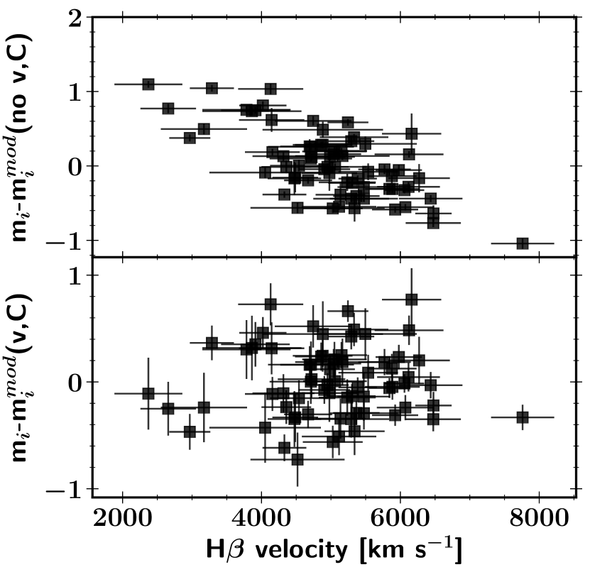
Figure 7: The relationship between SN II luminosity and the ejecta expansion velocity 43 d after the explosion. The upper panel shows the relationship (SN II magnitudes are corrected for distances and colours), while the lower panel shows the trend between luminosity and velocity after correcting the magnitudes for velocities ($\alpha\,\mathrm{log_{10}}v_{\mathrm{H\beta}}$).

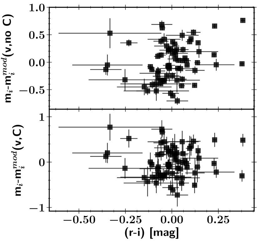
Figure 8: The relationship between SN II luminosity and the colour 43 d after the explosion. The upper panel shows the relationship (SN II magnitudes are corrected for distances and velocities), while the lower panel shows the trend between luminosity and colour after correcting the magnitudes for colours ($\beta(r-i)$).

4.2 Sample comparisons

We note that in the Hubble diagram plotted in Figure 5, there is an average systematic offset of $\sim 0.28$ mag between SDSS-II and DES-SN: for SDSS-II, the average residual from the $\Lambda$CDM model is $-0.22$ mag while for DES-SN it is 0.06 mag. First, as suggested by D’Andrea et al. (2010) and Poznanski et al. (2010), this offset could be due to a selection effect where brighter objects were favoured by SDSS-II. SDSS-II was built for SN Ia cosmology; thus, the spectroscopic follow-up program was designed for SNe Ia, which are more luminous than SNe II, so only the brightest SNe II would have been spectroscopically followed. In Section 4.5 we calculate a $\mu$-bias correction to account for effects such as Malmquist bias, based on simulations of each survey. In an ideal world, that correction would remove selection effects like those caused by the SDSS-II follow-up strategy. However, our $\mu$-bias simulation is only an approximation, and in the future it should be calculated more accurately using better SN II templates, and with the infrastructure to model SN II spectral features and their correlations with brightness. Second, this discrepancy could arise from photometric calibration errors (e.g., zero-points). We investigated possible calibration errors by checking the photometric system zero-point using different spectrophotometric standard stars. We also checked our methodology (Milky Way extinction, K/S correction; see Section 2.1) by comparing two SN II magnitudes observed by CSP-I and SDSS-II. In their natural photometric systems, a clear offset is seen between the CSP-I and SDSS-II photometry (e.g., $i$ band: $\sim-0.12$ mag), while after applying our correction (Milky Way extinction, K/S correction; see Section 2.1), the offset disappears and the photometry is consistent (e.g., $i$ band: $\sim-0.02$ mag). Third, we compare the SDSS distance moduli derived in this work and those by Poznanski et al. (2010). We find good agreement and an average difference of 0.05 mag which is much lower than the uncertainties. All of our tests confirm our methodology; hence, as with D’Andrea et al. (2010) and Poznanski et al. (2010), we believe that this offset is due to a selection effect where only bright SNe II have been spectroscopically observed and our current $\mu$-bias simulation cannot correct it. We have estimated the potential cosmological impact of this offset and found it to be significantly smaller than the current uncertainties, but it will become important for future analyses.

We show that SDSS is biased toward bright objects; thus, to investigate if the DES-SN sample comes from a progenitor population similar to that of the other SN II samples, we compare their velocity and absolute magnitude (without applying velocity or dust correction and assuming a $\Lambda$CDM model) distributions to those of the other samples.

Figure 9 (upper) shows the H$\beta$ velocity distribution. Although the DES-SN sample distribution looks slightly different from the CSP-I (no peak around 6000 km s^-1), a Kolomogorov-Smirnov test does not reject the null hypothesis that both groups are sampled from populations with identical distributions ($p=0.66$). Therefore, all of the velocity distributions are consistent with coming from the same distribution. In addition, all of the surveys have similar average velocities. Figure 9 (lower) shows the absolute magnitude distribution. There we see that the DES-SN sample distribution is similar to the CSP-I sample, while the SDSS-II sample distribution statistically differs ($p=0.012$) with an average absolute magnitude brighter than for CSP-I. As discussed above, D’Andrea et al. (2010) and Poznanski et al. (2010) suggested that the SDSS-II sample is biased toward brighter objects.

This is also seen in the $\Omega_{m}$ values obtained using CSP-I + SDSS-II and CSP-I + DES-SN (see Table 3). With CSP-I + SDSS-II, because SDSS-II is biased toward brighter objects, $\Omega_{m}$ is larger than using CSP-I + DES-SN ($0.66^{+0.25}_{-0.37}$ versus $0.30^{+0.35}_{-0.21}$). These distributions show that the DES-SN sample has a different or less extreme bias than SDSS II (see Section 4.5), explaining why the best-fitting parameters are consistent with or without the DES-SN sample.

To determine whether we see any evolution effects on the fitting parameters, we fit our data using different samples (see Section 4.5 for bias simulation). All of the best-fitting values and their associated uncertainties are displayed in Table 3. The easiest way to look for potential redshift effects is to compare the parameters derived using only the local CSP-I sample and the most distant SNe II from a combination of the SDSS-II, SNLS, DES-SN, and HSC samples. Both subsamples have roughly the same size (37 versus 33 SNe II). Even if the best-fitting parameters are consistent at 1$\sigma$ owing to their large uncertainties, we see variations between the two subsamples, suggesting possible redshift effects. However, we think that the differences could be explained by a bias selection (Malmquist) rather than by redshift evolution. This trend was also found in previous studies (Nugent et al., 2006; D’Andrea et al., 2010; Poznanski et al., 2010) when they compared their low-$z$ and high-$z$ samples. For example, D’Andrea et al. (2010) and Poznanski et al. (2010) found that the SDSS-II sample was overluminous and favoured a smaller value of $\alpha$.

Regarding the effect of host-galaxy extinction, we do not find a statistically significant correlation between the $(r-i)$ colour at 43 d and the redshift. However, even if the colour scatter is large and the order of magnitude of the K-correction is $\sim 0.02$ mag for CSP-I or $\sim 0.12$ mag for SDSS-II/DES-SN (depending on the SN redshift and filters), a possible trend is seen. Most distant SNe II seem to have smaller $(r-i)$ values (bluer objects). We find an average colour of $0.003\pm 0.119$ mag ($N=39$), $-0.072\pm 0.106$ mag ($N=24$), and $-0.134\pm 0.185$ mag ($N=7$) for $z<0.05$, $0.05<z<0.15$, and $z>0.15$, respectively. This could be an effect of the Malmquist bias; at high-$z$ we observe the brightest events, those less affected by host-galaxy extinction. However, as demonstrated in the previous paragraph, the colour has a tiny effect on the SN II standardisation, suggesting that the trend is more due to noise than a correlation between the redshift and the colour. Nonetheless, it could also be caused by intrinsic properties (de Jaeger et al., 2018).

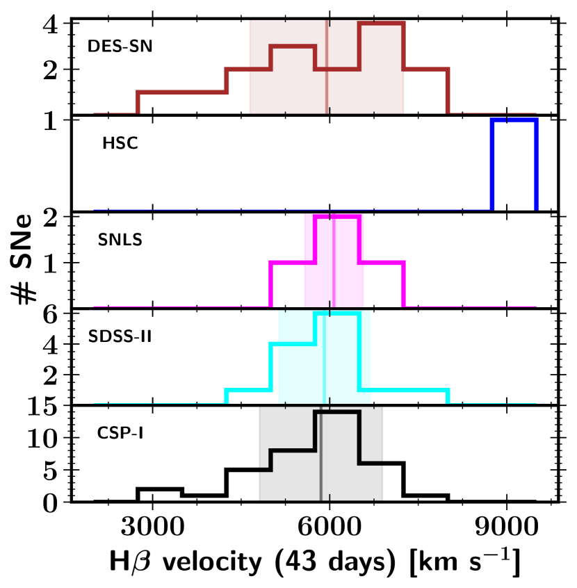
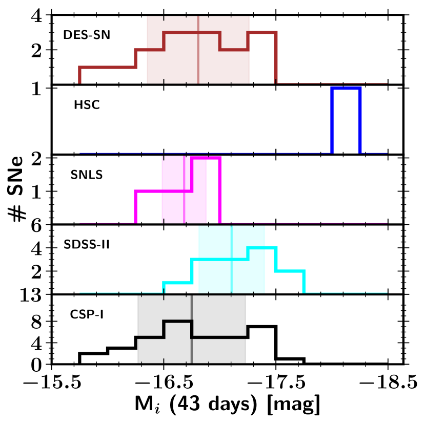
Figure 9: Upper: Histograms of the H$\beta$ velocities in km s^-1 measured using the cross-correlation technique for the CSP-I (black), SDSS-II (cyan), SNLS (magenta), HSC (blue), and DES-SN (brown) surveys. Lower: Distribution of the absolute $i$-band magnitude at 43 d of the CSP-I (black), SDSS-II (cyan), SNLS (magenta), HSC (blue), and DES-SN (brown) surveys. The absolute magnitudes were calculated assuming a $\Lambda$CDM model ($\Omega_{m}=0.30$, $\Omega_{\Lambda}=0.70$) and a Hubble constant of 70 km s^-1 Mpc^-1. Readers are reminded that the HSC sample had only one SN. In both figures, the vertical line and the filled region represent the median and their 1$\sigma$ uncertainties, respectively.

Table 3: SCM-fit parameters: samples

Dataset	$\alpha$	$\beta$	$M_{i}$	$\sigma_{\rm int}$	$\Omega_{m}$	$N$(SNe)
CSP-I	3.82 ${}^{+0.68}_{-0.64}$	0.97 $\pm$ 0.45	$-$16.79 $\pm$ 0.06	0.29 ${}^{+0.05}_{-0.04}$	0.50 ${}^{+0.33}_{-0.34}$	37
CSP-I$+$SDSS-II	3.78 ${}^{+0.61}_{-0.59}$	0.93 ${}^{+0.35}_{-0.34}$	$-$16.87 $\pm$ 0.05	0.28 $\pm$ 0.05	0.66 ${}^{+0.25}_{-0.37}$	50
CSP-I$+$SNLS	3.68 ${}^{+0.64}_{-0.62}$	0.82 ${}^{+0.35}_{-0.34}$	$-$16.79 ${}^{+0.05}_{-0.05}$	0.29 ${}^{+0.05}_{-0.04}$	0.28 ${}^{+0.37}_{-0.21}$	41
CSP-I$+$DES-SN	3.64 ${}^{+0.54}_{-0.53}$	0.56 ${}^{+0.35}_{-0.34}$	$-$16.80 $\pm$ 0.05	0.29 $\pm$ 0.05	0.30 ${}^{+0.35}_{-0.21}$	52
CSP-I$+$SDSS-II$+$SNLS	3.64 ${}^{+0.61}_{-0.58}$	0.90 ${}^{+0.35}_{-0.34}$	$-$16.86 $\pm$ 0.05	0.29 $\pm$ 0.04	0.44 ${}^{+0.34}_{-0.30}$	54
CSP-I$+$SDSS-II$+$SNLS+HSC	3.79 $\pm$ 0.55	0.89 ${}^{+0.35}_{-0.33}$	$-$16.88 $\pm$ 0.05	0.29 $\pm$ 0.04	0.51 ${}^{+0.33}_{-0.30}$	55
de Jaeger et al. (2017a)	3.60 ${}^{+0.52}_{-0.51}$	0.91 ${}^{+0.31}_{-0.30}$	$-$16.92 $\pm$ 0.05	0.29 ${}^{+0.04}_{-0.03}$	0.38 ${}^{+0.31}_{-0.25}$	61
CSP-I$+$SDSS-II$+$DES-SN	3.63 ${}^{+0.51}_{-0.49}$	0.74 ${}^{+0.33}_{-0.32}$	$-$16.87 $\pm$ 0.05	0.29 $\pm$ 0.04	0.39 ${}^{+0.35}_{-0.27}$	65
CSP-I$+$SNLS$+$DES-SN	3.59 ${}^{+0.53}_{-0.52}$	0.47 ${}^{+0.39}_{-0.37}$	$-$16.80 $\pm$ 0.05	0.29 $\pm$ 0.04	0.23 ${}^{+0.30}_{-0.17}$	56
CSP-I$+$SDSS$+$SNLS$+$DES-SN$+$HSC	3.71 ${}^{+0.51}_{-0.49}$	0.71 ${}^{+0.32}_{-0.33}$	$-$16.88 $\pm$ 0.05	0.29 ${}^{+0.04}_{-0.03}$	0.35 ${}^{+0.33}_{-0.23}$	70
SDSS-II	3.84 ${}^{+1.39}_{-1.91}$	0.02 ${}^{+0.64}_{-0.58}$	$-$17.15 $\pm$ 0.09	0.20 $\pm$ 0.12	0.57 ${}^{+0.30}_{-0.36}$	13
SDSS-II$+$SNLS	2.22 ${}^{+1.88}_{-1.95}$	0.48 ${}^{+0.75}_{-0.77}$	$-$17.04 $\pm$ 0.10	0.34 ${}^{+0.10}_{-0.07}$	0.38 ${}^{+0.38}_{-0.27}$	17
SDSS-II$+$DES-SN	3.36 ${}^{+0.87}_{-0.85}$	0.26 ${}^{+0.52}_{-0.53}$	$-$16.97 ${}^{+0.09}_{-0.08}$	0.3 ${}^{+0.07}_{-0.06}$	0.31 ${}^{+0.37}_{-0.23}$	28
SDSS-II$+$SNLS$+$DES-SN	3.18 $\pm$ 0.83	0.25 ${}^{+0.50}_{-0.52}$	$-$16.94 $\pm$ 0.08	0.31 $\pm$ 0.06	0.27 ${}^{+0.36}_{-0.20}$	32
SDSS-II$+$SNLS$+$HSC$+$DES-SN	3.56 ${}^{+0.80}_{-0.78}$	0.26 ${}^{+0.52}_{-0.54}$	$-$16.97 ${}^{+0.09}_{-0.08}$	0.30 $\pm$ 0.06	0.33 ${}^{+0.37}_{-0.24}$	33
SNLS$+$DES-SN	3.40 $\pm$ 0.89	$-$0.46 ${}^{+0.58}_{-0.62}$	$-$16.73 $\pm$ 0.10	0.25 ${}^{+0.09}_{-0.08}$	0.5 ${}^{+0.34}_{-0.33}$	19
DES-SN	3.35 $\pm$ 1.01	$-$0.38 ${}^{+0.68}_{-0.65}$	$-$16.76 $\pm$ 0.11	0.30 ${}^{+0.11}_{-0.09}$	0.50 ${}^{+0.34}_{-0.33}$	15

Best-fitting values and the associated uncertainties for each parameter of the SCM fit at 43 d after the explosion and using different samples.

4.3 Fit for $\Omega_{m}$ in $\Lambda$CDM cosmological model

After constructing a high-$z$ Hubble diagram assuming a fixed cosmology, here we constrain cosmological parameters. We follow the procedure presented in Section 4.1 with the exception of leaving $\Omega_{m}$ as a free parameter together with $\alpha$, $\beta$, $\mathcal{M}_{i}$, and $\sigma_{\rm obs}$. The best-fitting parameters ($\alpha$, $\beta$, $\mathcal{M}_{i}$, $\sigma_{\rm obs}$, and $\Omega_{m}$) are shown in Figure 10 in a corner plot with all of the one- and two-dimensional posterior distributions.

The fitted value for the matter density is $\Omega_{m}=0.35^{+0.33}_{-0.23}$, which corresponds to a dark energy density of $\Omega_{\Lambda}=0.65^{+0.24}_{-0.33}$. The value derived in this work is consistent with that obtained by de Jaeger et al. (2017a) ($\Omega_{m}=0.38^{+0.31}_{-0.25}$) and demonstrates evidence of dark energy using SNe II. Despite this independent measurement, the precision reached with SNe II is far from that obtained with SNe Ia (Betoule et al., 2014; Scolnic et al., 2018). A more precise estimate of the cosmological parameters requires a significant improvement of the SCM (see Section 4.1) and an increase in the number of high-$z$ SN II observations. In this sample, only three SNe II have been observed at $z>0.3$ while many hundreds of high-$z$ SNe Ia have been used for cosmology (Betoule et al., 2014; Scolnic et al., 2018).

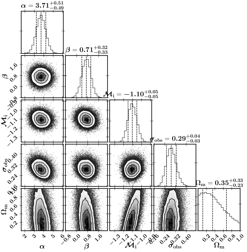
Figure 10: Corner plot showing all of the one- and two-dimensional projections. Contours are shown at 0.5$\sigma$, 1$\sigma$, 1.5$\sigma$, and 2$\sigma$ (which, in two dimensions, correspond to the 12%, 39%, 68%, and 86% of the volume). The five free parameters are plotted: $\alpha$, $\beta$, $\mathcal{M}_{i}$, $\sigma_{\rm obs}$, and $\Omega_{m}$. To make this figure we used the corner plot package (triangle.py v0.1.1. Zenodo. 10.5281/zenodo.11020); we assume a flat universe and use the SCM.

4.4 Error budget

In this section, we analyse the effect of each systematic error on the distance modulus. We run a Monte Carlo (MC) simulation ($N=2000$ realisations), where for each simulation, only one systematic (explosion date, magnitude, velocity, etc.) is offset by a random error (Gaussian distribution) due to its uncertainty. Then, for each iteration, the data are fitted using Eq. 3 (without Bayes’ inference as it was performed in Section 4.1 and 4.3 – i.e., only a likelihood minimisation without priors). New values of $\alpha$, $\beta$, $\mathcal{M}_{i}$, $\sigma_{\rm obs}$, and $\Omega_{m}$ are derived, and therefore new distance moduli as well. Finally, we compare the average distance moduli obtained with those derived without MC simulation. The effect on the fitting parameters of each systematic uncertainty is summarised in Table 4. Note that the fitting parameters at 43 d shown in Table 4 slightly differ from those displayed in Figure 10, as the former are derived only by minimising Eq. 3 without running an MCMC simulation.

4.4.1 Zero-point uncertainties

Ground-based photometric zero-point calibration is generally limited to an accuracy of 0.01–0.02 mag (see Table 10 of Conley et al. 2011). To compute the zero-point uncertainty effects on the distance modulus, for each survey we shift in turn the photometry from each band by 0.015 mag (Amanullah et al., 2010) and refit. All of the fitting parameters and the distance moduli remain essentially similar. If we use different offset for each survey (Conley et al., 2011), only $\Omega_{m}$ changes slightly (see Table 4).

4.4.2 Magnitude/colour uncertainties

The changes of the distance moduli and the fitting parameters due to the uncertainties in the photometry are evaluated by applying a magnitude/colour offset within the errors and refitting the data. The average fitting parameters and their standard deviation are shown in Table 4. As expected, $\beta$ is the fitting parameter with the largest difference, as it is the one which multiplies the colour term. The distance modulus residual between the values obtained with and without MC simulation has an average difference of 0.02 mag. A strong correlation is seen between the distance modulus residuals and the colours in the sense that bluer SNe II have larger positive residuals.

4.4.3 Photospheric velocity uncertainties

Here we investigate the influence of the photospheric velocity uncertainties on the distance moduli. We offset all of the velocities by a random error and refit all the data. We perform a MC analysis with 2000 realisations. The fitting parameter and distance modulus values and uncertainties correspond to the average value and the standard deviation over these 2000 realisations and are displayed in Table 4. The most affected fitting parameters are $\alpha$ and $\Omega_{m}$. This is easily explained by the fact that $\alpha$ is the parameter which multiplies the velocity. Regarding the distance modulus residual, the average of the absolute value is 0.038 mag with a maximum of 0.12 mag for SN 2008br. A strong correlation is seen between the distance modulus residuals and the velocities, in the sense that SNe with higher velocities have positive and larger residuals, while SNe with smaller velocities have negative and smaller residuals.

4.4.4 Explosion date

Explosion date uncertainties are among the most important systematic errors, as they affect all of the observables: magnitudes, colours, and expansion velocities. In order to quantify the effect on the distance modulus, we compare the distance moduli derived at 43 d (see Section 4.1) with those derived at 43 d plus a random value within a normal distribution due to the uncertainty (MC simulation, $N=2000$).

In Table 4, the average fitting parameters and their standard deviations are displayed. A comparison of the distance moduli obtained at 43 d and those derived here gives a maximum difference of $\sim 0.1$ mag, while the average absolute difference is $\sim 0.035$ mag – that is, $\sim 18$% of the average distance modulus uncertainties ($\sim 0.20$ mag; excluding the observed dispersion of 0.30 mag). This is not surprising, as the distributions are centred on 43 d, and thus the average distance moduli are also centred on the correct values derived in Section 4.1). However, we can look at the SNe II with the largest differences (SN 2008br, SN 2008hg, DES14C3rhw, DES17S1bxt, and SN 2016jhj). One SN II (SN 2008br) has a large explosion date uncertainty (9 d), while for the other SNe II, the uncertainties are all $\leq 5$ d. However, both DES14C3rhw and DES17S1bxt have large magnitude/colour uncertainties, and SN 2016jhj has a steeply declining plateau. We can also compare the scatter around the mean value and the uncertainty in the distance modulus itself. Six SNe II have a scatter larger than the uncertainty: SN 2005dt, SN 2007W, SN 2008ag, SN 2008bu, SN 2009bu, and 04D1pj. All of these SNe II have relatively large explosion date uncertainties: 9, 7, 8, 7, 8, and 8 d, respectively.

Finally, it is important to note that with our methodology, two effects affect the distance modulus: the explosion date and the explosion-date uncertainty. In Figure 4, we study the explosion-date effect by showing $\Omega_{m}$ for different epochs. We clearly see that $\Omega_{m}$ varies depending on the epoch at which we apply the method. At 30–40 d after the explosion, $\Omega_{m}\approx 0.2$–0.3, while at later epoch (70 d), the value increases to $\sim 0.7$. Even if the value changes, almost all of the values are consistent at 1$\sigma$ owing to their large uncertainties. We also look at the evolution of the fitting parameters using different epochs (between 40 and 70 d after the explosion). All of the fitting parameters evolve with the reference epoch; for example, $\alpha=2.42\pm 0.49$ when the reference epoch is 55 d. Finally, it is interesting to note that as for the velocity uncertainties, the same correlation is seen between the distance modulus residuals and the velocities. This could be explained by the fact that $\alpha$ is the one of the most affected fitting parameters.

4.4.5 Gravitational lensing

Gravitational lensing only affects the high-redshift part of the Hubble diagram, leading to potential bias of the cosmological parameters. However, even if for our sample ($z<0.36$) gravitational lensing should not have a strong effect, we adopt the approach of Conley et al. (2011); Betoule et al. (2014); Scolnic et al. (2018) by adding a value of 0.055$z$ (Jönsson et al., 2010) in quadrature to the total uncertainty (see Eq. 3). Other studies (e.g., Kowalski et al. 2008; Amanullah et al. 2010) treat gravitational lensing using a value of 0.093$z$ (Holz & Linder, 2005). Including the gravitational lensing term in the total uncertainty increases the average distance modulus uncertainties by 0.01 mag.

4.4.6 Minimum redshift

To evaluate for possible effects from using a given minimum redshift cut ($z_{\rm CMB}>0.01$), we construct a new sample including all of the SNe II, with no minimum redshift. The new sample size increases to 82 SNe II (instead of 70 SNe II). A systematic offset of $\sim 0.02$ mag is seen between the distance moduli derived using the whole sample and the cut sample. The fitting parameters $\alpha$ and $\beta$ slightly differ because their velocity and colour distribution centres are similar. However, $\mathcal{M}_{i}$ varies when including all the SNe with a difference of almost 1$\sigma$. If we change the redshift cut to $z_{\rm CMB}>0.0223$ (the cut used by Riess et al. 2016), the sample decreases to 44 SNe II and the fitting parameters change as seen in Table 4. A difference of $\sim 0.6$, $\sim 0.7$, $\sim 1.4$, $\sim 0.2$, and $0.3\sigma$ for (respectively) $\alpha$, $\beta$, $\mathcal{M}_{i}$, $\sigma_{\rm obs}$, and $\Omega_{m}$ is seen.

4.4.7 Milky Way extinction

All of the light curves were corrected for Milky Way extinction using the Cardelli et al. (1989) law, assuming a total-to-selective extinction ratio of $R_{V}=3.1$ and using the extinction maps of Schlafly & Finkbeiner 2011. To quantify the Milky Way extinction uncertainty effects on the distance modulus, we follow the approach of (Amanullah et al., 2010), increasing the Galactic $E(B-V)$ by 0.01 mag for each SN and repeating the fit. All of the fitting parameters and the distance moduli are almost identical; the distance modulus residual has an average of $4.0\times 10^{-4}$ mag.

Table 4: SCM-fit parameters: systematics errors.

Systematic errors	$\alpha$	$\beta$	$\mathcal{M}_{i}$	$\sigma_{\rm int}$	$\Omega_{m}$
Original	3.77 $\pm$ 0.51	0.76 $\pm$ 0.32	$-$1.13 $\pm$ 0.06	0.27 $\pm$ 0.04	0.17 $\pm$ 0.35
ZP	3.76 $\pm$ 0.51	0.77 $\pm$ 0.32	$-$1.11 $\pm$ 0.06	0.27 $\pm$ 0.03	0.19 $\pm$ 0.36
Mag/colour	3.75 $\pm$ 0.51	0.61 $\pm$ 0.34	$-$1.12 $\pm$ 0.06	0.28 $\pm$ 0.04	0.24 $\pm$ 0.39
Velocity	3.29 $\pm$ 0.56	0.75 $\pm$ 0.35	$-$1.11 $\pm$ 0.06	0.30 $\pm$ 0.04	0.30 $\pm$ 0.42
$t_{\rm exp}$	3.47 $\pm$ 0.62	0.60 $\pm$ 0.37	$-$1.11 $\pm$ 0.07	0.30 $\pm$ 0.04	0.31 $\pm$ 0.45
All $z$	3.82 $\pm$ 0.47	0.78 $\pm$ 0.32	$-$1.06 $\pm$ 0.04	0.29 $\pm$ 0.04	0.21 $\pm$ 0.37
$z>0.0223$	4.14 $\pm$ 0.71	0.36 $\pm$ 0.43	$-$1.25 $\pm$ 0.05	0.27 $\pm$ 0.05	0.05 $\pm$ 0.42
$A_{V,G}$	3.77 $\pm$ 0.51	0.77 $\pm$ 0.32	$-$1.11 $\pm$ 0.05	0.27 $\pm$ 0.04	0.17 $\pm$ 0.35
mean systematic	0.17 $\pm$ 0.18	0.11 $\pm$ 0.25	0.04 $\pm$ 0.04	0.01 $\pm$ 0.01	0.08 $\pm$ 0.05

Effect of the systematic errors on the best-fitting values using the SCM. Original line corresponds to the values obtained by minimising Eq. 3 without MCMC (no Bayesian inference). Velocity, $t_{\rm exp}$, All $z$, $z>0.0223$, $A_{V,G}$, ZP (shift separately for each survey), and Mag/colour correspond to the values derived by changing the velocities, explosion time, including all the redshifts, including only the SNe II with $z>0.0223$, the Galactic visual extinction, the filter photometric zero-point, and the colour/magnitude as described in Section 4.4. Note that for each parameter, the total errors correspond to the standard deviation of the 2000 MC simulations added in quadrature to the mean of the 2000 errors obtained for each parameter. The mean systematic uncertainty corresponds to the average of the difference between the original and each systematic, while the error corresponds to the standard deviation.

4.5 Simulated distance modulus bias versus redshift

In this section, we will use the public “SuperNova ANAlysis” (SNANA) software package (Kessler et al., 2009) to estimate the distance modulus bias ($\mu$-bias) due to selection effects (e.g., Malmquist bias) versus redshift. As seen in Figure 1 where the overall number of events exponentially declines with redshift, the Malmquist bias could be significant and an important source of uncertainty (see Section 4.4).

To simulate events, SNANA needs three ingredients (Kessler et al., 2019b; Brout et al., 2019b): (1) a source model, to generate a variety of spectral energy distributions (SEDs); (2) a noise model, to convert true magnitudes to true fluxes with a certain cadence, and apply Poisson noise to get measured fluxes; and (3) a trigger model, to define the final sample by applying spectroscopic selection functions or candidate logic (e.g., at least two detections).

As a source model, we use the “SNII-NMF” model used for the Photometric LSST Astronomical Time Series Classification Challenge (PLAsTiCC; Kessler et al. 2019a). It consists of a SED, which is a linear combination of three “eigenvectors” built using hundreds of well-observed SNe II after applying a non-negative matrix factorisation (NMF) as a dimensionality reduction technique. For each simulated SN II, the multiplicative factors of the three “eigenvectors” (“eigenvalues”) are obtained from correlated Gaussian distributions measured from the data.

Unlike the SN Ia bias simulation in Kessler et al. (2019b), for SNe II we do not have the infrastructure to model spectral features and their correlations with brightness (e.g., expansion velocities vs. brightness); thus, we apply a slightly different methodology. First, we assume that the total rest-frame brightness variation is $\sim 0.95$ mag, and second, that after standardisation the Hubble scatter is 0.27 mag. Therefore, to model the magnitude variation, we will use two sources: a known random scatter with a dispersion of 0.815 mag (the SNII-NMF model by itself includes a scatter of 0.4 mag) which is exactly corrected in the analysis, and an unknown intrinsic scatter with a dispersion of 0.27 mag. Note that the combined dispersion is 0.95 mag. Both scatters are added coherently to all bands and phases (COH model).

SNANA can directly use the image properties (PSF, sky noise, zero point) to simulate the noise; however, other than for DES-SN, we do not have access to the meta data to perform these accurate simulations. Therefore, we follow the procedure described by Kessler et al. (2019b) (in their Section 6.1.1) for their low-$z$ sample. Instead of using the image properties, an approximate cadence is generated directly from the observed data (light curves, redshifts, coordinates, observation dates, etc.).

The last step (trigger model) is to apply the spectroscopic selection function. For each survey, it consists of a function of peak $i$-band magnitude versus redshift. This function is manually adjusted until good agreement between simulations and data for redshift and Milky Way extinction (MW $E(B-V)$) distributions is obtained. As seen in Figure 11, we find good agreement between the data and simulations for all surveys and for both redshift and MW $E(B-V)$ parameters. Note that for each survey, we simulated 1,000,000 objects; 2.4%, 1.3%, 1.8%, and 2.6% (CSP-I, SDSS-II, SNLS, and DES-SN, respectively) of the objects passed the spectroscopic selection.

Finally, the $\mu$-bias versus redshift is obtained by taking the average value of the random Gaussian smear applied in the simulation corresponding to the unknown scatter (dispersion of 0.27 mag). In Figure 12, $\mu$-bias versus redshift is shown for four surveys: CSP-I, SDSS-II, SNLS, and DES-SN. The average $\mu$-bias for the CSP-I survey is $\sim-0.15$ mag, while for SDSS, the $\mu$-bias is lower with an average value of $\sim-0.09$ mag. From these simulations, we see that the SN II $\mu$-bias increase can be large at high redshifts, with a value of $\sim-0.25$ mag at $z=0.3$.

It is important to note that the SN II bias is much larger than the one obtained for SNe Ia. With their low-$z$ sample, Kessler et al. (2019b) obtained an average value of $\sim-0.02$ mag. Even if one expects to obtain a larger bias for SNe II than for SNe Ia because SN II are less luminous (by $\sim 2$ mag), the large difference is also due to a difference in the methodology. If the same technique used in this work is applied to the low-$z$ SN Ia sample from Kessler et al. (2019b), the average SN Ia bias increases to $-0.10$ mag. To obtain a more accurate $\mu$-bias simulation, the spectral features and their correlations with brightness need to be modeled, as well as the use of a better SN II template; this is matter for future work.

Even though our method is an approximation, we apply the $\mu$-bias to each SN II and refit the cosmology. Note that for the HSC sample, we use the SNLS bias. The best-fitting parameters obtained with bias correction are consistent with those obtained without. For example, we derive $\Omega_{m}=0.29^{+0.32}_{-0.20}$ versus $\Omega_{m}=0.35^{+0.33}_{-0.23}$ (see Section 4.3). Regarding the other parameters, we get $\alpha=3.52\pm 0.49$ (versus $\alpha=3.71^{+0.51}_{-0.49}$), $\beta=0.66\pm 0.33$ (versus $\beta=0.71^{+0.32}_{-0.33}$), and $\mathcal{M}_{i}=-1.00\pm 0.05$ (versus $\mathcal{M}_{i}=-1.10\pm 0.05$), with an observed dispersion $\sigma_{\rm obs}=0.29^{+0.04}_{-0.03}$ mag (versus $\sigma_{\rm obs}=0.29^{+0.04}_{-0.03}$ mag). With these new fitting-parameter values, the offset between SDSS and DES seen in Figure 5 remains the same ($\sim 0.28$ mag). If we fixed $\alpha$, $\beta$, and $\mathcal{M}_{i}$, and apply the $\mu$-bias correction, the SDSS average offset reduces to $-0.13$ mag but the DES average offset increases to 0.15 mag, and therefore the offset between SDSS and DES remains almost identical.

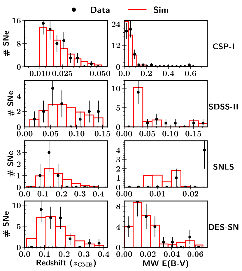
Figure 11: Comparison of data (black dots) and simulation using SNANA (red histogram) for distributions in the CSP-I (top row), SDSS-II (second row), SNLS (third row), and DES-SN (bottom row) samples. The simulations have 1,000,000 SNe for each survey, but the histograms were scaled to have the same number of events as the data. The left column shows CMB redshift $z_{\rm CMB}$, while the right column represents Galactic extinction MW $E(B-V)$.

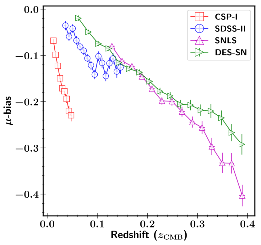
Figure 12: Distance modulus bias due to selection effects versus redshift for CSP-I (red squares), SDSS-II (blue circles), SNLS (magenta triangles), and DES-SN (green right-pointed triangles).

5 PCM Results

In this section, we will first assume a $\Lambda$CDM cosmological model and present an updated SN II Hubble diagram using the PCM. Second, assuming a flat universe, we will constrain the matter density ($\Omega_{m}$). In both cases, a comparison with photometric Hubble diagrams from the literature is presented. Note that, unlike for the SCM, in this Section we do not perform $\mu$-bias simulation. We leave a detailed modelisation of the photometric features and their correlations with brightness to a future paper as it will require a significant effort to update SNANA.

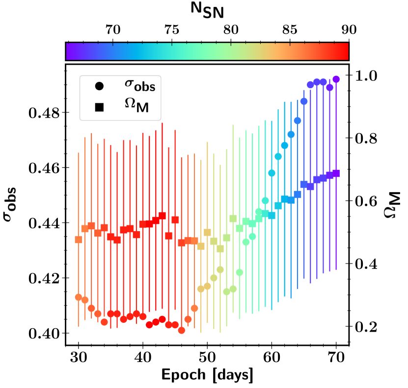
Figure 13: Variation by epoch of the intrinsic dispersion in the Hubble diagram (circles and left ordinate axis) and $\Omega_{m}$ (squares and right ordinate axis) using the PCM. The colour bar at the top represents the different sample sizes. For clarity, only the $\Omega_{m}$ uncertainties are plotted.

5.1 Fixed cosmology

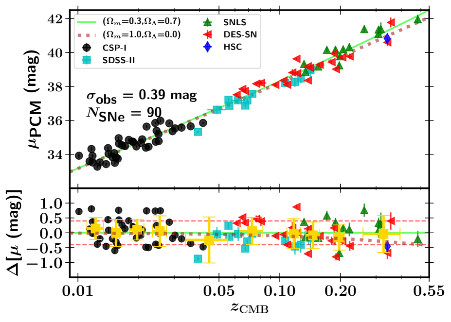
Figure 14: Hubble diagram (top) and residuals from the $\Lambda$CDM model (bottom) using the PCM as applied to the data taken from CSP-I (black circles; de Jaeger et al. 2017b), SDSS-II (cyan squares; D’Andrea et al. 2010), SNLS (green triangles; de Jaeger et al. 2017b), HSC (blue diamond; de Jaeger et al. 2017a), and DES-SN (red left triangles; this work). The lime solid line is the Hubble diagram for the $\Lambda$CDM model ($\Omega_{m}=0.3$, $\Omega_{\Lambda}=0.7$), while the brown dot line is for an Einstein-de Sitter cosmological model ($\Omega_{m}=1.0$, $\Omega_{\Lambda}=0.0$). In both models, we use H${}_{0}=70$ km s^-1 Mpc^-1 to standardise the SN II brightness. We present the number of SNe II available at this epoch ($N_{\rm SNe}$), the epoch after the explosion, and the observed dispersion ($\sigma_{\rm obs}$). The yellow squares in the Hubble residual plot represent the binned data using 10 SNe II per bin.

As for the SCM, we select SNe II in the Hubble flow – a total of 101 SNe II (47 CSP-I $+$ 14 SDSS-II $+$ 15 SNLS $+$ 1 HSC $+$ 24 DES-SN). We apply the PCM at 43 d after the explosion even if at 46 d the scatter is slightly smaller as shown in Figure 13. This choice is motivated by the fact that between the two epochs the intrinsic dispersion differs by 0.003 mag but at 43 d the comparison with the SCM will be straightforward. From the total sample we cut 8 SNe II because their explosion date uncertainties are larger than 10 d (see Table 2), 2 SNe II for a lack of photometry, and 1 SN II (DES13C2jtx) identified as an outlier ($3\sigma$ clipping).

Finally, the PCM total sample at 43 d is composed of 90 SNe II: 40 SNe II from CSP-I, 13 SNe II from SDSS-II, 14 SNe II from SNLS, 1 SN II from HSC, and 22 SNe II from DES-SN.

In Figure 14 the SN II Hubble diagram and the Hubble residuals of the combined data are shown. Assuming a $\Lambda$CDM cosmological model, the best-fitting parameters are $\alpha=0.24\pm 0.06$, $\beta=0.53\pm 0.31$, and $\mathcal{M}_{i}=-1.05\pm 0.05$, with an observed dispersion $\sigma_{\rm obs}=0.39\pm 0.04$ mag, or 17–18% in distance. As shown in Figure 15, almost all the fitting parameters are consistent at 1$\sigma$ with those derived by de Jaeger et al. (2017b) ($\alpha=0.36\pm 0.06$, $\beta=0.71^{+0.29}_{-0.28}$, $\mathcal{M}_{i}=-1.08\pm 0.05$, and $\sigma_{\rm obs}=0.36\pm 0.03$ mag). However, difference are seen in $\alpha$ and could be explained by the newly reanalysed $s_{2}$ values for the whole sample (Galbany et al., in prep.). For all the surveys, the $s_{2}$ distributions are displayed in Figure 16. The DES-SN sample distribution is statistically (KS test) consistent with the other distributions. Using the PCM, the average systematic offset between SDSS-II and DES-SN ($\sim 0.28$ mag) seen in Figure 5 is smaller. For SDSS, the median residual from the $\Lambda$CDM model is $-0.17$ mag while for DES-SN it is $-0.01$ mag.

We also compare the distance moduli derived in this work and those by de Jaeger et al. (2017b). A mean difference of $-0.02$ mag with a standard deviation of 0.24 mag is found. 14 SNe II (9 from CSP-I, 3 from SDSS-II, and 2 from SNLS) have distance moduli not consistent at 1$\sigma$, 5 SNe II (4 from CSP-I and 1 from SNLS) at 2$\sigma$, and 2 SNe II from CSP-I at 3$\sigma$. These differences could be attributed to a difference of methodology (linear interpolation versus Gaussian Process), to a fine-tuned measurement of $s_{2}$ (mean average difference of $-0.05$ mag (100 d)^-1), but mostly by the use of the recalibrated CSP-I photometry (14/19 SNe II are from CSP). However, it is important to note that if we take into account the minimum uncertainty in distance determination using the PCM ($\sim 0.40$ mag), all the distances are consistent.

Finally, in Figure 17 and Figure 18, the relationship between the two parameters ($s_{2}$ and colour) that have been used to standardise SNe II and the luminosity are shown. From these figures as seen with the SCM, the colour does not improve the standardisation. The Pearson factor between the colour and the luminosity corrected for distance and $s_{2}$ is 0.21 and decreases to 0.03 after correction. On the other hand, a correlation is seen between $s_{2}$ and the magnitude corrected for distance and colour with a Pearson factor of $-0.43$. The $s_{2}$ coefficient is efficient, as the Pearson factor drops to $-0.02$ when a $s_{2}$ correction is applied.

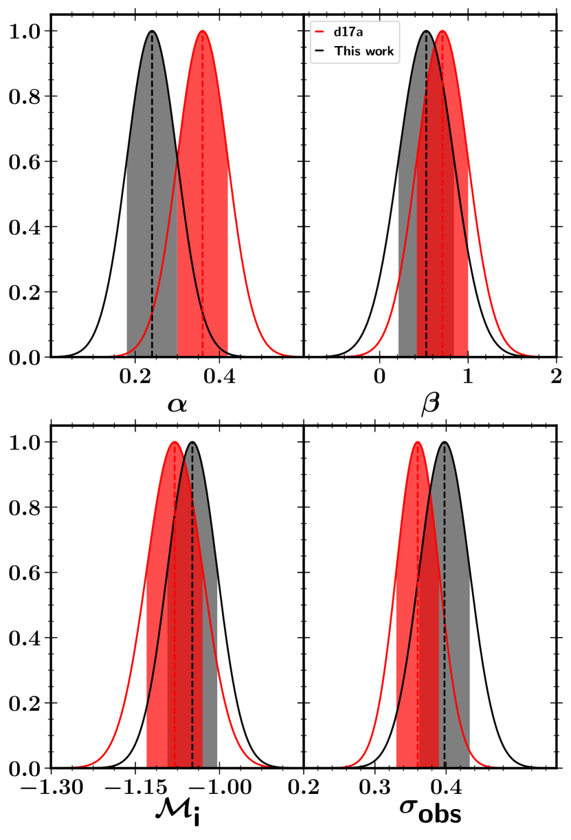
Figure 15: Comparison of the best-fitting parameters using the PCM derived by de Jaeger et al. (2017b) in red and those obtained in this work (in black) with the DES-SN sample. Top left: Distributions of $\alpha$. Top right: Distributions of $\beta$. Bottom left: Distributions of “Hubble-constant-free” absolute magnitude ($\mathcal{M}_{i}$). Bottom right: Distributions of observed dispersion ($\sigma_{\rm obs}$). In each panel, the vertical dashed line represents the average value, while the filled region represents the 1$\sigma$ uncertainty.

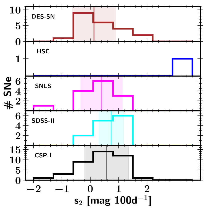
Figure 16: Histograms of the $s_{2}$ slope in mag (100 d)^-1 for the CSP-I (black), SDSS-II (cyan), SNLS (magenta), HSC (blue), and DES-SN (brown) surveys. Readers are reminded that the HSC sample had only one SN. The vertical lines and the filled regions represent the medians and their 1$\sigma$ uncertainties, respectively.

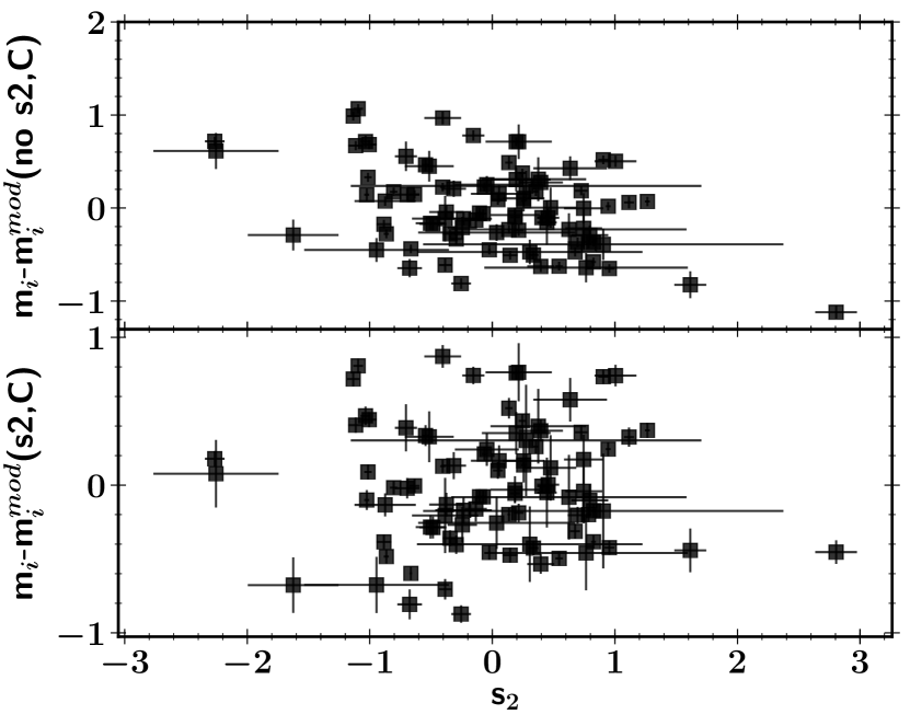
Figure 17: The relationship between SN II luminosity and $s_{2}$. The upper panel illustrates the relationship (SN II magnitudes are corrected for distances and colours), while the lower panel shows the trend between luminosity $s_{2}$ after correcting the magnitudes for $s_{2}$ ($\alpha s_{2}$).

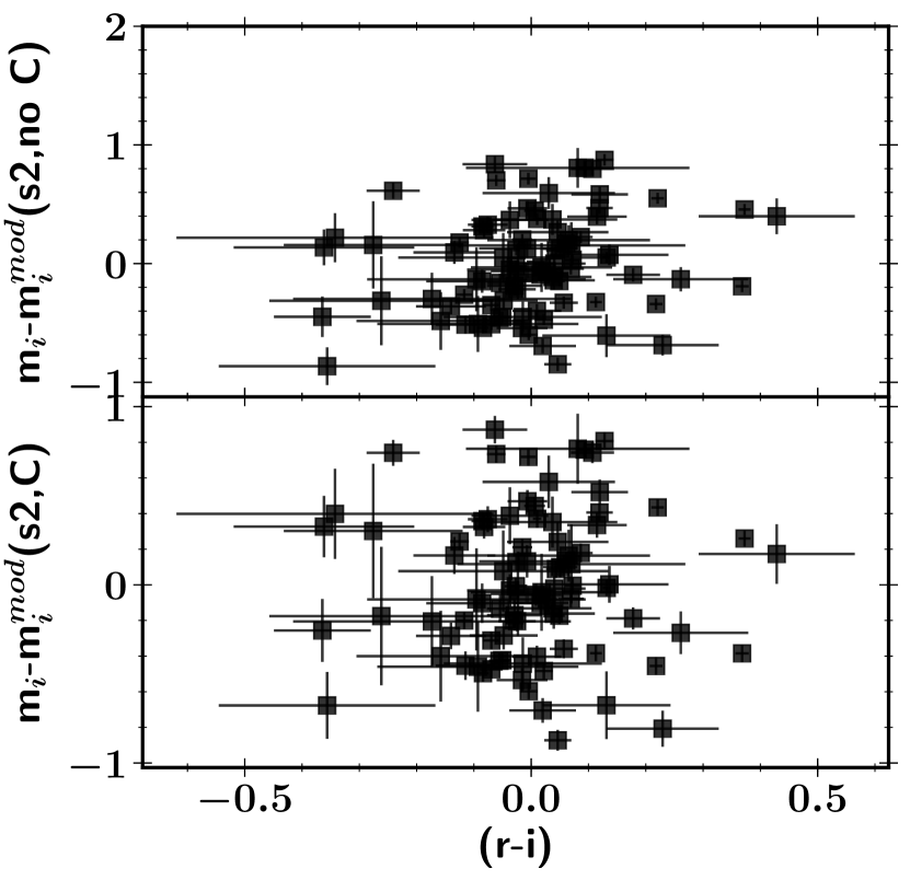
Figure 18: The relationship between SN II luminosity and the colour 43 d after the explosion. The upper panel shows the relationship (SN II magnitudes are corrected for distances and $s_{2}$), while the lower panel shows the trend between luminosity colour after correcting the magnitudes for colours ($\beta$$(r-i)$).

5.2 $\Omega_{m}$ derivation

Following the procedure described in Section 4.3, we also derive an $\Omega_{m}$ value assuming a flat universe. In Figure 19, a corner plot with all the one- and two-dimensional projections is shown. Assuming a flat universe, we derive a value for the matter density of $\Omega_{m}=0.62^{+0.24}_{-0.29}$ – that is, a dark energy density value $\Omega_{\Lambda}=0.38^{+0.29}_{-0.24}$. Even if this result is almost consistent at 1$\sigma$ with the latest SN Ia results (Scolnic et al. 2018; $\Omega_{m}=0.298\pm 0.022$), our $\Omega_{m}$ value is much larger. It is also important to note that this result appears to be affected by the priors. If we choose less restrictive priors for $\Omega_{m}$, $0.0<\Omega_{m}<2.5$ instead of $0.0<\Omega_{m}<1.0$, the value and the uncertainties increase to $\Omega_{m}=0.77^{+0.46}_{-0.36}$. Both values are consistent owing to their large uncertainties; however, the fact that $\Omega_{M}$ depends on the priors could suggest that currently with our small sample of high-$z$ SNe II, SNe II cannot play a key role in the $\Omega_{M}$ determination and should be used only at low-$z$ to derive H₀. In the future, though, more SNe II will be observed at high-$z$, and this larger set of SNe II will be useful for estimating $\Omega_{M}$.

With respect to de Jaeger et al. (2017b) – that is, the same sample except the DES-SN and HSC samples – in this work we found a higher value (but still consistent) for the matter density ($\Omega_{m}=0.32^{+0.30}_{-0.21}$ in de Jaeger et al. 2017b). This might be explained by the fact that the DES-SN sample could be biased toward brighter objects, implying smaller distances and thus, by definition, favouring a Universe with more matter. However, as discussed in Section 4.2, it does not seem to be the case. Even if using the PCM our results are larger than the current best-fit values from other probes, we think that this method is still encouraging as it allows us to use more objects (only those with photometric information). However, future work should focus on reducing the intrinsic dispersion by (for example) developing a new SN II template for the K-correction or to fit the light curves and measure more precisely the $s_{2}$ slopes and the magnitudes. Finally, new improvements could also be possible by adding another parameter which correlates with the intrinsic brightness or by finding a SN II subgroup which is better standardisable. Note that if we use the velocity and the slope term, the dispersion does not decrease and remains around 0.28–0.30 mag.

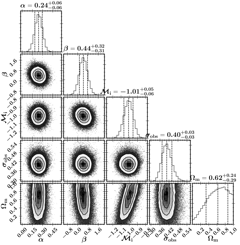
Figure 19: Corner plot showing all of the one- and two-dimensional projections. Contours are shown at 0.5$\sigma$, 1$\sigma$, 1.5$\sigma$, and 2$\sigma$ (which, in two dimensions, correspond to the 12%, 39%, 68%, and 86% of the volume). The five free parameters are plotted: $\alpha$, $\beta$, $\mathcal{M}_{i}$, $\sigma_{\rm obs}$, and $\Omega_{m}$. To make this figure we use the corner-plot package (triangle.py v0.1.1. Zenodo. 10.5281/zenodo.11020). In deriving this figure, we assume a flat universe.

5.3 Redshift bias

As done with the SCM, here we determine if there is any bias effect as a function of the redshift. We fit our data using different samples and all the best-fitting values are shown in Table 5. From this table, a possible redshift evolution is seen in $\alpha$. A value of $0.30\pm 0.09$ is found for the low-$z$ sample (CSP-I; 40 SNe II) while $\alpha=0.19\pm 0.07$ using the rest of the sample (SDSS-II $+$ SNLS $+$ DES-SN $+$ HSC; 49 SNe II) or $\alpha=0.07^{+0.10}_{-0.09}$ for SNLS $+$ DES-SN. Values at low-$z$ and high-$z$ differ by $\sim 1\sigma$; therefore, this difference could be explained by a redshift evolution or by a Malmquist bias (at high-$z$ the brightest objects are observed). In any case, further investigations with better statistics at high-$z$ should be done to confirm or invalidate this result. Regarding the $\beta$ value, the large uncertainties prevent a definitive conclusion; however, at first sight, the values remain around 0.4 except for SNLS $+$ DES-SN where a smaller but still consistent value is found. Finally, the $\Omega_{m}$ values obtained using CSP-I $+$ SDSS-II and CSP-I $+$ DES-SN are more similar for the PCM than the SCM which confirms the absence of an offset in the Hubble diagram for the PCM (see Figure 14).

Table 5: PCM-fit parameters.

Dataset	$\alpha$	$\beta$	$M_{i}$	$\sigma_{\rm int}$	$\Omega_{m}$	SNe
CSP-I	0.29 $\pm$ 0.09	0.33 ${}^{+0.62}_{-0.60}$	$-$16.75 $\pm$ 0.07	0.43 ${}^{+0.06}_{-0.05}$	0.52 ${}^{+0.33}_{-0.35}$	40
CSP-I$+$SDSS-II	0.26 $\pm$ 0.08	0.65 $\pm$ 0.47	$-$16.83 $\pm$ 0.06	0.41 ${}^{+0.05}_{-0.04}$	0.64 ${}^{+0.26}_{-0.37}$	53
CSP-I$+$SNLS	0.24 $\pm$ 0.08	0.30 $\pm$ 0.46	-16.73 $\pm$ 0.07	0.41 ${}^{+0.05}_{-0.04}$	0.38 ${}^{+0.33}_{-0.25}$	54
CSP-I$+$DES-SN	0.25 $\pm$ 0.07	0.39 $\pm$ 0.41	$-$16.73 $\pm$ 0.06	0.42 $\pm$ 0.04	0.72 ${}^{+0.20}_{-0.30}$	62
CSP-I$+$SDSS-II$+$SNLS	0.23 $\pm$ 0.07	0.41 $\pm$ 0.39	$-$16.79 $\pm$ 0.06	0.40 ${}^{+0.04}_{-0.03}$	0.37 ${}^{+0.33}_{-0.25}$	67
CSP-I$+$SDSS-II$+$SNLS+HSC	0.26 ${}^{+0.06}_{-0.07}$	0.51 ${}^{+0.39}_{-0.40}$	$-$16.82 $\pm$ 0.06	0.40 $\pm$ 0.04	0.44 ${}^{+0.32}_{-0.27}$	68
CSP-I$+$SDSS-II$+$DES-SN	0.24 $\pm$ 0.07	0.56 $\pm$ 0.35	$-$16.79 $\pm$ 0.05	0.41 ${}^{+0.04}_{-0.03}$	0.74 ${}^{+0.19}_{-0.31}$	75
CSP-I$+$SNLS$+$DES-SN	0.22 ${}^{+0.07}_{-0.06}$	0.28 ${}^{+0.36}_{-0.34}$	$-$16.71 $\pm 0.06$	0.41 ${}^{+0.04}_{-0.03}$	0.59 ${}^{+0.26}_{-0.29}$	76
CSP-I$+$SDSS$+$SNLS$+$DES-SN$+$HSC	0.24 $\pm$ 0.06	0.44 ${}^{+0.32}_{-0.31}$	$-$16.78 $\pm$ 0.05	0.40 $\pm$ 0.03	0.62 ${}^{+0.24}_{-0.29}$	90
SDSS-II	0.07 ${}^{+0.19}_{-0.18}$	0.40 ${}^{+0.76}_{-0.79}$	$-$17.14 $\pm$ 0.12	0.33 ${}^{+0.11}_{-0.07}$	0.50 ${}^{+0.33}_{-0.34}$	13
SDSS-II$+$SNLS	0.11 $\pm$ 0.11	0.45 ${}^{+0.55}_{-0.61}$	$-$16.94 ${}^{+0.10}_{-0.09}$	0.37 ${}^{+0.07}_{-0.06}$	0.17 ${}^{+0.29}_{-0.13}$	27
SDSS-II$+$DES-SN	0.18 $\pm$ 0.10	0.57 ${}^{+0.47}_{-0.45}$	$-$16.87 $\pm$ 0.09	0.41 ${}^{+0.06}_{-0.05}$	0.60 ${}^{+0.28}_{-0.34}$	35
SDSS-II$+$SNLS$+$DES-SN	0.15 $\pm$ 0.08	0.39 $\pm$ 0.39	$-$16.83 ${}^{+0.09}_{-0.08}$	0.40 ${}^{+0.05}_{-0.04}$	0.40 ${}^{+0.35}_{-0.27}$	49
SDSS-II$+$SNLS$+$DES-SN$+$HSC	0.21 $\pm$ 0.07	0.44 $\pm$ 0.39	$-$16.83 $\pm$ 0.09	0.40 ${}^{+0.05}_{-0.04}$	0.50 ${}^{+0.31}_{-0.30}$	50
SNLS$+$DES-SN	0.09 ${}^{+0.10}_{-0.09}$	0.04 $\pm$ 0.46	$-$16.66 ${}^{+0.09}_{-0.10}$	0.39 ${}^{+0.06}_{-0.05}$	0.68 ${}^{+0.23}_{-0.33}$	36
DES-SN	0.163 $\pm$ 0.14	0.27 ${}^{+0.64}_{-0.62}$	$-$16.71 ${}^{+0.11}_{-0.12}$	0.44 ${}^{+0.09}_{-0.07}$	0.70 ${}^{+0.22}_{-0.35}$	22

Best-fitting values and the associated uncertainties for each parameter of the PCM fit at 43 d after the explosion and using different samples.

5.4 Error budget

As previously done in Section 4.4, in this section, we analyse the effect of each systematic error on the distance modulus. We follow the same procedure explained above, running an MC simulation where for each simulation each observable is offset by a value according to its uncertainty. The effect on the fitting parameters of each systematic error is summarised in Table 6. For reference, we use the fitting parameters obtained at 43 d derived by minimising 3 (without MCMC).

5.4.1 Zero-point uncertainties

Similarly to the method used for the SCM, here we compute the zero-point uncertainty effects on the distance modulus by shifting in turn the photometry from each band by 0.015 mag and refit (Amanullah et al., 2010). Almost all the fitting parameters and the distance moduli remain identical, only $\mathcal{M}_{i}$ change to $-$98 $\pm$ 0.07. If instead of adding a constant value for all the photometric systems, we add a different offset for each survey (Conley et al., 2011), $\Omega_{m}$ evolves slightly but not statistically significantly (increase of 0.02, $<3\%$) as seen in Table 6,.

5.4.2 Magnitude/colour uncertainties

To estimate the influence of the photometry uncertainty, we apply a magnitude/colour offset within the error uncertainties and refit the data (2000 simulations). The average fitting parameters and their associated standard deviations are shown in Table 6. The only fitting parameter statistically affected by the photometric uncertainties is $\beta$. An absolute average difference of 0.013 mag is seen in the distance moduli, and as for the SCM, the distance modulus residuals and the colours are correlated in the sense that bluer SNe II have larger positive residuals.

5.4.3 Slope uncertainties

In this paragraph, the effect of the plateau slope uncertainties on distance moduli are investigated. We offset the slope by a number withing the slope uncertainty and refit all the data. The average and standard deviation of the 2000 fitting parameters are displayed in 6. All of the fitting parameters remain mostly identical. Even $\alpha$ which multiplies the slope almost does not change. Therefore, the absolute average distance modulus difference is very small (0.01 mag) and the maximum value is 0.05 mag. A strong correlation is seen between the distance modulus residuals and the slope, in sense that SNe with steeper slope have positive and larger residuals.

5.4.4 Explosion date

Following the procedure described in Section 4.4.4, we investigate the explosion date uncertainty effects on the fitting parameters and the distance moduli. For this purpose, we apply the PCM not at 43 d but at 43 d plus a random value within a normal distribution due to the explosion date uncertainty which is different for each SN. In Table 6, the averaged fitting parameters and their standard deviation are displayed. The distance moduli derived using the PCM are less affected by the explosion date uncertainty than those obtained with the SCM. The average absolute difference in the distance moduli is $\sim 0.012$ mag against 0.035 mag for the SCM. This is easily explained as for the SCM, the expansion velocities are strongly affected by the explosion date while for the PCM, the plateau slope is not. This is seen in Figure 4 where the $\Omega_{m}$ values at different epoch is displayed. For the PCM, the $\Omega_{m}$ evolves from $\sim 0.50$ at early epochs to $\sim 0.70$ at late time, while for the SCM the variation was larger ($\sim 0.20$ to $\sim 0.70$). Regarding the fitting parameters, only $\beta$ and $\Omega_{m}$ evolve, but they are still consistent at 1$\sigma$ with the “original” values.

5.4.5 Gravitational lensing

As for the SCM, the gravitational lensing effects are treated by adding a value of 0.055$z$ (Jönsson et al., 2010) in quadrature to the total uncertainty (see Eq. 3). If we choose another value (e.g., 0.093$z$ Kowalski et al. 2008), the total uncertainty on the distance modulus increase by 0.01 mag.

5.4.6 Minimum redshift

In this subsection, the effects on the fitting parameters on using a give redshift cut ($z_{\rm CMB}>0.01$) are analysed. For this purpose, we change the redshift cut to $z_{\rm CMB}>0.0223$, the same cut used by Riess et al. (2016). The sample decreases from 90 SNe II to 63 SNe II. As seen in Table 6, all of the fitting parameters change: $\sim 12$% for $\alpha$, $\sim 10$% for $\mathcal{M}_{i}$, and $\sim 40$% for $\Omega_{m}$. The distance moduli are different with an absolute average difference of 0.08 mag.

5.4.7 Milky Way extinction

Following (Amanullah et al., 2010), we evaluate the Milky Way extinction uncertainty effects on the distance modulus by increasing the Galactic $E(B-V)$ by 0.01 mag for each SN and repeat the fit. As shown in Table 6, all the fitting parameters remain almost identical, and therefore, the distance moduli too.

Table 6: PCM-fit parameters: systematics errors.

Systematic errors	$\alpha$	$\beta$	$\mathcal{M}_{i}$	$\sigma_{\rm int}$	$\Omega_{m}$
Original	0.24 $\pm$ 0.05	0.42 $\pm$ 0.32	$-$1.00 $\pm$ 0.07	0.39 $\pm$ 0.03	0.68 $\pm$ 0.39
ZP	0.24 $\pm$ 0.05	0.42 $\pm$ 0.32	$-$0.98 $\pm$ 0.07	0.39 $\pm$ 0.03	0.70 $\pm$ 0.39
Mag/colour	0.24 $\pm$ 0.06	0.32 $\pm$ 0.32	$-$0.99 $\pm$ 0.07	0.40 $\pm$ 0.03	0.72 $\pm$ 0.41
slope	0.22 $\pm$ 0.06	0.45 $\pm$ 0.33	$-$1.00 $\pm$ 0.07	0.39 $\pm$ 0.03	0.67 $\pm$ 0.39
$t_{\rm exp}$	0.25 $\pm$ 0.06	0.34 $\pm$ 0.35	$-$1.00 $\pm$ 0.07	0.40 $\pm$ 0.04	0.61 $\pm$ 0.40
All $z$	0.24 $\pm$ 0.05	0.45 $\pm$ 0.32	$-$0.99 $\pm$ 0.07	0.38 $\pm$ 0.03	0.74 $\pm$ 0.41
$z<0.0223$	0.21 $\pm$ 0.07	0.41 $\pm$ 0.37	$-$1.10 $\pm$ 0.09	0.38 $\pm$ 0.04	0.40 $\pm$ 0.39
$A_{V,G}$	0.24 $\pm$ 0.05	0.42 $\pm$ 0.32	$-$0.98 $\pm$ 0.07	0.39 $\pm$ 0.03	0.67 $\pm$ 0.38
mean systematic	0.01 $\pm$ 0.01	0.04 $\pm$ 0.04	0.02 $\pm$ 0.03	0.006 $\pm$ 0.005	0.07 $\pm$ 0.09

Effect of the systematic errors on the best-fitting values using the PCM. Original line corresponds to the values obtained by minimising Eq. 3 without MCMC (no Bayesian inference), while slope, $t_{\rm exp}$, All $z$, $z>0.0223$, $A_{V,G}$, ZP (shift separately for each survey), and Mag/colour respectively correspond to the values derived by changing the slopes, explosion time, including all the redshifts, including only the SNe II with $z>0.0223$, the filter photometric zero-point, and the colour/magnitude as described in Section 5.4. Note that for each parameter, the total errors correspond to the standard deviation of the 2000 MC simulations added in quadrature to the mean of the 2000 errors obtained for each parameter. The mean systematic uncertainty corresponds to the average of the difference between the original and each systematic while the error corresponds to the standard deviation.

5.5 SCM versus PCM

In this Section, we compare the intrinsic dispersion and the distance moduli obtained applying the SCM and the PCM. For this purpose, we restrict the PCM sample to the SNe II in common with those used with the SCM: 70 SNe II. Figure 20 shows a comparison of the Hubble diagrams obtained with both method. As we can see, the distance moduli derived with the SCM and PCM are almost all consistent with a median absolute difference of 0.15 mag, much lower than the intrinsic dispersion of both methods ($\sim 0.3$ and $\sim 0.4$ mag). Though the distance moduli are similar, the intrinsic dispersion is different. The SCM is a better method to standardise the SNe II than the PCM with a difference of $\sim 0.1$ mag, or $\sim 5$% in distance. However, spectroscopic follow-up observations for all events discovered by the next generation of surveys will be impossible, and more work should be done to try to improve a photometric method as for example developing a new SN II template for SN II light-curve fitting.

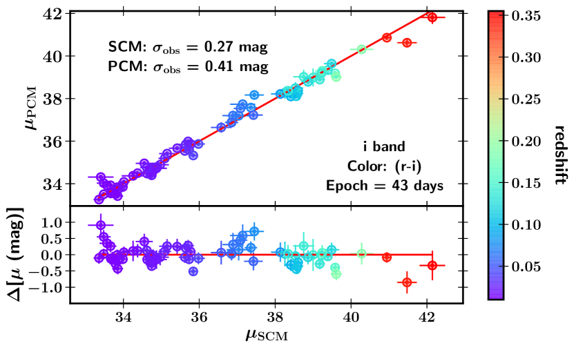
Figure 20: Comparison between the distance moduli measured from the SCM and those determined from the PCM. The residuals are plotted in the bottom panel. The red solid line represents a slope of unity while the colour bar on the right side represents the different redshifts. We present the observed dispersion ($\sigma_{\rm obs}$) of both methods.

6 Conclusions

Using the DES-SN combined with four other surveys (CSP-I, SDSS-II, SNLS, and HSC), we perform the most complete SN II cosmology analysis and construct the two largest Hubble diagrams with SNe II in the Hubble flow. First, using the SCM at 43 d after the explosion – epoch which minimises the intrinsic dispersion and maximises the number of objects – and 70 SNe II we find an intrinsic dispersion in the Hubble diagram of 0.27 mag which is consistent with previous studies. We derive cosmological parameters ($\Omega_{m}=0.35^{+0.33}_{-0.23}$) consistent with the $\Lambda$CDM model and the accelerated expansion of the Universe. We demonstrate that the colour term does not improve the SN II standardisation and solely the expansion velocity correction is enough. This would be an asset as only one photometric band and one spectrum are necessary to calibrate the SN II. This leaves room for the possibility of a new correlation which will help to improve the standardisation.

For the first time in SN II cosmology, a SN II distance modulus bias simulation using SNANA is performed and we show that the best-fitting parameters are not affected. Second, to take advantage of the next generation of surveys and their thousands of thousands SN II discoveries, we apply a purely photometric method (PCM). We construct a Hubble diagram with a redshift range up to $\sim 0.5$ and an observed scatter of 0.39 mag, or 17–18% in distances. Both methods demonstrate a promising future for SNe II as distance indicators and their utility at low-$z$ to derive H₀. However, we address the important needs for building a survey mainly dedicated to SN II cosmology as the majority of the current surveys were concentrated on SN Ia cosmology (e.g., noisy spectra). Additionally, future work should focus on building a SN II template to perform K-corrections and to develop a SN II light-curve fitter. Currently, SNe II are not competitive with SN Ia in term of precision, but with these improvements, we will have the real capacity to compare them with the SNe Ia and see if they can or cannot play a key role in cosmology.

7 Affiliations

¹ Department of Astronomy, University of California, 501 Campbell Hall, Berkeley, CA 94720-3411, USA.
² Bengier Postdoctoral Fellow.
³ Departamento de Física Teórica y del Cosmos, Universidad de Granada, E-18071 Granada, Spain.
⁴ CENTRA, Instituto Superior Técnico, Universidade de Lisboa, Av. Rovisco Pais 1, 1049-001 Lisboa, Portugal.
⁵ Department of Astronomy and Astrophysics, University of Chicago, Chicago, IL 60637, USA.
⁶ Kavli Institute for Cosmological Physics, University of Chicago, Chicago, IL 60637, USA.
⁷ Miller Senior Fellow, Miller Institute for Basic Research in Science, University of California, Berkeley, CA 94720, USA.
⁸ Millennium Institute of Astrophysics (MAS), Nuncio Monseñor Sótero Sanz 100, Providencia, Santiago, Chile.
⁹ Center for Mathematical Modeling, Universidad de Chile, Santiago, Chile.
¹⁰ Departamento de Astronomía – Universidad de Chile, Camino el Observatorio 1515, Santiago, Chile.
¹¹ George P. and Cynthia Woods Mitchell Institute for Fundamental Physics & Astronomy, Mitchell Physics Building, Texas A. & M. University, USA.
¹² School of Mathematics and Physics, University of Queensland, Brisbane, QLD 4072, Australia.
¹³ School of Physics and Astronomy, University of Southampton, Southampton, SO17 1BJ, UK.
¹⁴ School of Physics & Astronomy, Cardiff University, Queens Buildings, The Parade, Cardiff, CF24 3AA, UK.
¹⁵ Sydney Institute for Astronomy, School of Physics, A28, The University of Sydney, NSW 2006, Australia.
¹⁶ Université Clermont Auvergne, CNRS/IN2P3, LPC, F-63000 Clermont-Ferrand, France.
¹⁷ Department of Physics, Duke University Durham, NC 27708, USA.
¹⁸ Department of Physics and Astronomy, University of Pennsylvania, Philadelphia, PA 19104, USA.
¹⁹ INAF, Astrophysical Observatory of Turin, I-10025 Pino Torinese, Italy.
²⁰ Santa Cruz Institute for Particle Physics, Santa Cruz, CA 95064, USA.
²¹ Centre for Astrophysics & Supercomputing, Swinburne University of Technology, Victoria 3122, Australia.
²² Institute of Cosmology and Gravitation, University of Portsmouth, Portsmouth, PO1 3FX, UK.
²³ The Research School of Astronomy and Astrophysics, Australian National University, ACT 2601, Australia.
²⁴ Cerro Tololo Inter-American Observatory, National Optical Astronomy Observatory, Casilla 603, La Serena, Chile.
²⁵ Departamento de Física Matemática, Instituto de Física, Universidade de São Paulo, CP 66318, São Paulo, SP, 05314-970, Brazil.
²⁶ Laboratório Interinstitucional de e-Astronomia - LIneA, Rua Gal. José Cristino 77, Rio de Janeiro, RJ - 20921-400, Brazil.
²⁷ Fermi National Accelerator Laboratory, P. O. Box 500, Batavia, IL 60510, USA.
²⁸ Instituto de Fisica Teorica UAM/CSIC, Universidad Autonoma de Madrid, 28049 Madrid, Spain.
²⁹ CNRS, UMR 7095, Institut d’Astrophysique de Paris, F-75014, Paris, France.
³⁰ Sorbonne Universités, UPMC Univ Paris 06, UMR 7095, Institut d’Astrophysique de Paris, F-75014, Paris, France.
³¹ Department of Physics and Astronomy, Pevensey Building, University of Sussex, Brighton, BN1 9QH, UK.
³² Department of Physics & Astronomy, University College London, Gower Street, London, WC1E 6BT, UK.
³³ Kavli Institute for Particle Astrophysics & Cosmology, P. O. Box 2450, Stanford University, Stanford, CA 94305, USA.
³⁴ SLAC National Accelerator Laboratory, Menlo Park, CA 94025, USA.
³⁵ Centro de Investigaciones Energéticas, Medioambientales y Tecnológicas (CIEMAT), Madrid, Spain.
³⁶ Department of Astronomy, University of Illinois at Urbana-Champaign, 1002 W. Green Street, Urbana, IL 61801, USA.
³⁷ National Center for Supercomputing Applications, 1205 West Clark St., Urbana, IL 61801, USA.
³⁸ Institut de Física d’Altes Energies (IFAE), The Barcelona Institute of Science and Technology, Campus UAB, 08193 Bellaterra (Barcelona) Spain.
³⁹ Institute for Fundamental Physics of the Universe, Via Beirut 2, 34014 Trieste, Italy.
⁴⁰ INAF-Osservatorio Astronomico di Trieste, via G. B. Tiepolo 11, Italy.
⁴¹ Institut d’Estudis Espacials de Catalunya (IEEC), 08034 Barcelona, Spain.
⁴² Institute of Space Sciences (ICE, CSIC), Campus UAB, Carrer de Can Magrans, s/n, 08193 Barcelona, Spain.
⁴³ Observatório Nacional, Rua Gal. José Cristino 77, Rio de Janeiro, RJ-20921-400, Brazil.
⁴⁴ Department of Physics, IIT Hyderabad, Kandi, Telangana 502285, India.
⁴⁵ Department of Astronomy/Steward Observatory, University of Arizona, 933 North Cherry Avenue, Tucson, AZ 85721-0065, USA.
⁴⁶ Jet Propulsion Laboratory, California Institute of Technology, 4800 Oak Grove Dr., Pasadena, CA 91109, USA.
⁴⁷ Department of Physics, Stanford University, 382 Via Pueblo Mall, Stanford, CA 94305, USA.
⁴⁸ Department of Physics, ETH Zurich, Wolfgang-Pauli-Strasse 16, CH-8093 Zurich, Switzerland.
⁴⁹ Center for Cosmology and Astro-Particle Physics, The Ohio State University, Columbus, OH 43210, USA.
⁵⁰ Department of Physics, The Ohio State University, Columbus, OH 43210, USA.
⁵¹ Center for Astrophysics $|$ Harvard & Smithsonian, 60 Garden Street, Cambridge, MA 02138, USA.
⁵² Australian Astronomical Optics, Macquarie University, North Ryde, NSW 2113, Australia.
⁵³ Lowell Observatory, 1400 Mars Hill Rd, Flagstaff, AZ 86001, USA.
⁵⁴ Department of Astrophysical Sciences, Princeton University, Peyton Hall, Princeton, NJ 08544, USA.
⁵⁵ Observatories of the Carnegie Institution for Science, 813 Santa Barbara St., Pasadena, CA 91101, USA.
⁵⁶ Institució Catalana de Recerca i Estudis Avançats, E-08010 Barcelona, Spain.
⁵⁷ Department of Physics, University of Michigan, Ann Arbor, MI 48109, USA.
⁵⁸ Brandeis University, Physics Department, 415 South Street, Waltham MA 02453, USA.
⁵⁹ Computer Science and Mathematics Division, Oak Ridge National Laboratory, Oak Ridge, TN 37831, USA.
⁶⁰ Max Planck Institute for Extraterrestrial Physics, Giessenbachstrasse, 85748 Garching, Germany.
⁶¹ Universitäts-Sternwarte, Fakultät für Physik, Ludwig-Maximilians Universität München, Scheinerstr. 1, 81679 München, Germany.

Appendix A

List of the 56 spectroscopically classified SNe II from the DES-SN survey. For each SN, we indicate whether it did (“SCM”) or did not pass the cut. The SNe that failed are marked with “PHOT” (not enough data), “EXP” (no explosion date), “SPEC” (no spectrum), “P-Cygni” (no clear P-Cygni profile), and “LC” (unusual light curves).

Table 7: Spectroscopically classified SNe II.

SN	$z_{\rm CMB}$	Cut	Comments
DES13C2jtx	0.2234	P-Cygni
DES13C3ui	0.0663	EXP
DES13X3fca	0.0951	SCM
DES14C3aol	0.0764	SCM
DES14C3nm	0.3096	EXP
DES14C3rhw	0.3412	SCM
DES14C3tsg	0.2096	PHOT
DES14E2ar	0.0761	EXP
DES14X1qt	0.1380	EXP
DES14X2cy	0.2316	EXP
DES14X3ili	0.1412	P-Cygni
DES15C1okz	0.0696	PHOT
DES15C1pkx	0.1564	PHOT
DES15C2eaz	0.0612	SCM
DES15C2lna	0.0652	P-Cygni
DES15C2lpp	0.1806	P-Cygni	Classified as “SN II?”: ATel #8367
DES15C2npz	0.1221	SCM
DES15C3bj	0.2870	EXP	Classified as “SN II?”: ATel #8367
DES15E1iuh	0.1045	SCM
DES15E2ni	0.2253	EXP
DES15S1by	0.1283	EXP
DES15S1cj	0.1661	EXP	Classified as “SN II?”: ATel #8367
DES15S1lrp	0.2223	P-Cygni	Classified as “SN II?”: ATel #8658
DES15S2eaq	0.0672	SCM
DES15X1lzp	0.0792	SPEC
DES15X2mku	0.0807	SCM
DES15X3mpq	0.1872	P-Cygni
DES15X3nad	0.0998	P-Cygni
DES16C2cbv	0.1087	SCM
DES16C3at	0.2171	EXP
DES16E1ah	0.1480	EXP
DES16E1bkh	0.1155	P-Cygni
DES16S1gn	0.1899	SCM
DES16X1ey	0.0752	EXP
DES16X2bkr	0.1577	SCM
DES16X3cpl	0.2042	P-Cygni	Classified as “SN II?”: ATel #9742
DES16X3dvb	0.3292	LC	Slow rise and over luminous
DES16X3jj	0.2369	EXP	Classified as “SN II?”: ATel #9504
DES16X3km	0.0538	EXP
DES17C2pf	0.1358	EXP
DES17C3aye	0.1577	P-Cygni
DES17C3bei	0.1030	P-Cygni
DES17C3de	0.1070	EXP
DES17C3dw	0.1632	EXP
DES17E2bhj	0.1857	P-Cygni	Classified as “SN II?”: ATEL#11146
DES17E2cc	0.1478	EXP
DES17E2ci	0.1259	EXP
DES17S1bxt	0.3550	PHOT
DES17S1lu	0.0832	EXP
DES17S2oo	0.2243	EXP
DES17X1aow	0.1379	SCM
DES17X1axb	0.1377	SCM
DES17X1gd	0.1881	EXP	Classified as “SN II?”: ATel #11146
DES17X2ls	0.2509	EXP	Classified as “SN II?”: ATel #11147
DES17X3bd	0.1406	EXP	Classified as “SN II?”: ATel #10759
DES17X3dub	0.1210	SCM

Notes — Column 1, SN name; Column 2, heliocentric redshift; Column 3, sample cut: “SCM” (useful for cosmology), “PHOT” (not enough data), “EXP” (no explosion date), “SPEC” (no spectrum), “P-Cygni” (no clear P-Cygni profile), “LC” (unusual light curves); Column 4, comments.

Appendix B

All of the observed light curves for all SNe II with spectroscopic confirmation discovered by DES-SN and not included in the SCM sample are displayed in this Appendix. The spectra of the SNe II not used in our SCM sample owing to a lack of clear P-Cygni profiles are shown.

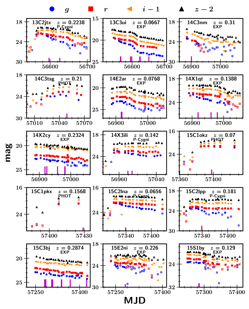
Figure 21: Observed light curves of all SNe II discovered by DES-SN with spectroscopic confirmation. Blue circles are $g$-band magnitudes, red squares are $r$, orange left triangles are $i-1$, and black top triangles are $z-2$. Empty symbols represent real points with flux/err $<3$.

The abscissa is the Modified Julian Date (MJD). In each panel, the IAU name and the redshift are given in the upper right. SNe that failed the cut are marked with “PHOT” (not enough data), “EXP” (no explosion date), “SPEC” (no spectrum), “P-Cygni” (no clear P-Cygni profile) , and “LC” (unusual light curves). The vertical magenta lines indicate the epochs of optical spectroscopy.

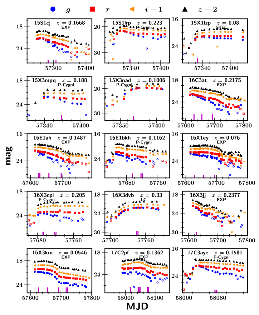
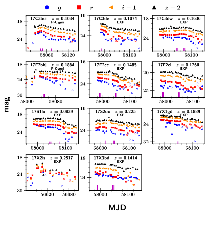
Figure 21: Observed light curves of all SNe II discovered by DES-SN with spectroscopic confirmation. Blue circles are $g$-band magnitudes, red squares are $r$, orange left triangles are $i-1$, and black top triangles are $z-2$. Empty symbols represent real points with flux/err $<3$.

The abscissa is the Modified Julian Date (MJD). In each panel, the IAU name and the redshift are given in the upper right. SNe that failed the cut are marked with “PHOT” (not enough data), “EXP” (no explosion date), “SPEC” (no spectrum), “P-Cygni” (no clear P-Cygni profile) , and “LC” (unusual light curves). The vertical magenta lines indicate the epochs of optical spectroscopy.

Figure 21: Observed light curves of all SNe II discovered by DES-SN with spectroscopic confirmation. Blue circles are $g$-band magnitudes, red squares are $r$, orange left triangles are $i-1$, and black top triangles are $z-2$. Empty symbols represent real points with flux/err $<3$.

The abscissa is the Modified Julian Date (MJD). In each panel, the IAU name and the redshift are given in the upper right. SNe that failed the cut are marked with “PHOT” (not enough data), “EXP” (no explosion date), “SPEC” (no spectrum), “P-Cygni” (no clear P-Cygni profile) , and “LC” (unusual light curves). The vertical magenta lines indicate the epochs of optical spectroscopy.

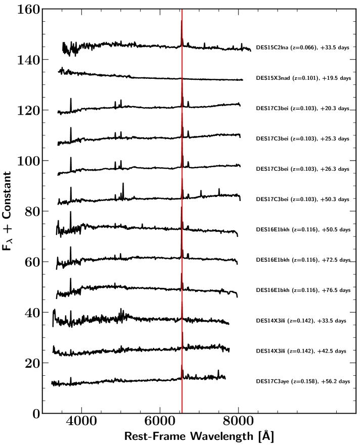
Figure 22: Spectra of the 12 SNe II from the DES-SN sample classified as “SN II” or “SN II?” but not included in the SCM sample because the P-Cygni profile is not clearly seen. The spectra are shown in the rest frame, and the date listed for each SN is the number of days since explosion. The redshift of each SN is labelled. The spectra were binned (10 Å). The red vertical line corresponds to H$\alpha$ ($\lambda$6563).

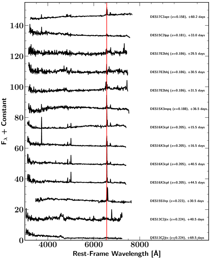
Figure 22: (Cont.) Spectra of the 12 SNe II from the DES-SN sample classified as “SN II” or “SN II?” but not included in the SCM sample because the P-Cygni profile is not clearly seen. The spectra are shown in the rest frame, and the date listed for each SN is the number of days since explosion. The redshift of each SN is labelled. The spectra were binned (10 Å). The red vertical line corresponds to H$\alpha$ ($\lambda$6563).

Appendix C

All DES-SN photometric and spectroscopic SN II data are publicly available at https://github.com/tdejaeger. The spectra are also available at the Weizmann Interactive Supernova Data Repository (WISeREP;https:/wiserep.weizmann.ac.il).

Table 8: DES-SN sample photometry.

SN name	MJD	$g$	$r$	$i$	$z$
		mag	mag	mag	mag
DES13C2jtx	56536.2	(25.221) $\pm$ (0.692)	(28.770) $\pm$ (3.814)	$\cdots$	$\cdots$
DES13C2jtx	56543.2	$\cdots$	(26.941) $\pm$ (1.420)	(26.738) $\pm$ (1.595)	$\cdots$
DES13C2jtx	56547.3	$\cdots$	(25.638) $\pm$ (0.806)	(27.438) $\pm$ (2.187)	$\cdots$
DES13C2jtx	56551.2	(26.517) $\pm$ (2.441)	$\cdots$	$\cdots$	$\cdots$
DES13C2jtx	56558.2	$\cdots$	$\cdots$	(24.188) $\pm$ (0.362)	$\cdots$
DES13C2jtx	56563.2	21.775 $\pm$ 0.023	22.155 $\pm$ 0.043	22.445 $\pm$ 0.066	22.653 $\pm$ 0.111
DES13C2jtx	56567.2	21.406 $\pm$ 0.016	21.554 $\pm$ 0.023	21.747 $\pm$ 0.034	21.786 $\pm$ 0.041
DES13C2jtx	56575.2	21.484 $\pm$ 0.015	21.488 $\pm$ 0.018	21.517 $\pm$ 0.023	21.674 $\pm$ 0.032
DES13C2jtx	56579.2	21.683 $\pm$ 0.039	21.641 $\pm$ 0.037	21.505 $\pm$ 0.034	21.774 $\pm$ 0.048
DES13C2jtx	56590.3	22.194 $\pm$ 0.077	21.733 $\pm$ 0.070	21.505 $\pm$ 0.061	21.729 $\pm$ 0.075
DES13C2jtx	56594.1	22.406 $\pm$ 0.066	21.834 $\pm$ 0.057	21.544 $\pm$ 0.057	21.781 $\pm$ 0.092
DES13C2jtx	56602.1	22.829 $\pm$ 0.042	21.968 $\pm$ 0.027	21.679 $\pm$ 0.028	21.944 $\pm$ 0.045
DES13C2jtx	56606.1	(23.407) $\pm$ (0.360)	22.262 $\pm$ 0.146	22.115 $\pm$ 0.155	22.136 $\pm$ 0.192
DES13C2jtx	56609.1	23.173 $\pm$ 0.184	22.004 $\pm$ 0.057	21.699 $\pm$ 0.042	21.878 $\pm$ 0.057
DES13C2jtx	56615.0	(23.332) $\pm$ (0.478)	22.436 $\pm$ 0.124	22.072 $\pm$ 0.116	22.228 $\pm$ 0.257
DES13C2jtx	56625.2	$\cdots$	22.442 $\pm$ 0.038	$\cdots$	$\cdots$
DES13C2jtx	56628.1	23.980 $\pm$ 0.151	22.437 $\pm$ 0.051	21.994 $\pm$ 0.045	22.117 $\pm$ 0.064
DES13C2jtx	56635.1	24.069 $\pm$ 0.193	22.654 $\pm$ 0.066	22.103 $\pm$ 0.055	22.219 $\pm$ 0.089
DES13C2jtx	56645.1	(24.638) $\pm$ (0.472)	22.648 $\pm$ 0.090	22.198 $\pm$ 0.063	22.368 $\pm$ 0.076
DES13C2jtx	56649.1	(25.097) $\pm$ (0.479)	22.832 $\pm$ 0.082	$\cdots$	$\cdots$
DES13C2jtx	56649.2	$\cdots$	$\cdots$	22.377 $\pm$ 0.072	22.448 $\pm$ 0.105
			$\cdots$
			$\cdots$

Notes: DES-SN SN II photometry. The values in parentheses are real points with flux/err $<3$. The table is only a fraction of a much larger table which covers each epoch of photometry for in SN. The full table is available in the online version of this article.

Table 9: Journal of spectroscopic observations of SN II DES-SN sample.

SN name	Date	MJD	Epoch	Telescope	Instrument	range
		UT	Days			Å
DES13C2jtx	2013-11-01	56597.0	40.5	AAT	AAOmega/2dF	3733–8855
DES13C2jtx	2013-11-30	56626.0	69.5	AAT	AAOmega/2dF	3733–8846
DES13X3fca	2013-10-30	56595.0	53.5	AAT	AAOmega/2dF	3733–8855
DES13X3fca	2013-11-03	56599.0	57.5	AAT	AAOmega/2dF	3733–8855
DES14C3aol	2014-10-29	56959.0	65.3	AAT	AAOmega/2dF	3734–8854
DES14C3rhw	2015-1-28	57050.0	47.5	VLT	X-Shooter	3400–10000
DES14X3ili	2014-11-18	56979.0	33.5	AAT	AAOmega/2dF	3734–8856
DES14X3ili	2014-11-27	56988.0	42.5	AAT	AAOmega/2dF	3734–8868
DES15C2eaz	2015-11-13	57339.0	68.5	AAT	AAOmega/2dF	3754–8922
DES15C2lna	2015-11-13	57339.0	33.5	AAT	AAOmega/2dF	3754–8859
DES15C2lpp	2015-11-13	57339.0	33.0	AAT	AAOmega/2dF	3754–8936
DES15C2npz	2016-01-11	57398.0	38.5	Magellan	LDSS3	4251–8669
DES15E1iuh	2015-10-13	57308.0	27.4	AAT	AAOmega/2dF	3754–8945
DES15E1iuh	2015-11-14	57340.0	59.4	AAT	AAOmega/2dF	3754–8945
DES15S1lrp	2015-11-12	57338.0	30.5	Magellan	LDSS3	4250–9330
DES15S2eaq	2015-12-03	57359.0	89.5	AAT	AAOmega/2dF	3757–8920
DES15X2mku	2015-12-14	57370.0	41.5	AAT	AAOmega/2dF	3753–8944
DES15X3mpq	2015-12-12	57368.0	36.5	AAT	AAOmega/2dF	3753–8944
DES15X3nad	2015-12-12	57368.0	19.5	AAT	AAOmega/2dF	3757–8920
DES16C2cbv	2016-11-03	57695.0	38.5	AAT	AAOmega/2dF	3905–8945
DES16C2cbv	2016-11-28	57720.0	63.5	AAT	AAOmega/2dF	3753–8944
DES16C2cbv	2016-11-29	57721.0	64.5	AAT	AAOmega/2dF	3753–8944
DES16E1bkh	2016-11-03	57695.0	50.5	AAT	AAOmega/2dF	3753–8906
DES16E1bkh	2016-11-25	57717.0	72.5	AAT	AAOmega/2dF	3753–8898
DES16E1bkh	2016-11-29	57721.0	76.5	AAT	AAOmega/2dF	3753–8898
DES16S1gn	2016-10-05	57666.0	46.5	AAT	AAOmega/2dF	3753–8945
DES16X2bkr	2016-11-03	57695.0	48.5	AAT	AAOmega/2dF	3753–8945
DES16X3cpl	2016-10-31	57692.0	15.5	AAT	AAOmega/2dF	3753–8931
DES16X3cpl	2016-11-01	57693.0	16.5	AAT	AAOmega/2dF	3753–8912
DES16X3cpl	2016-11-25	57717.0	40.5	AAT	AAOmega/2dF	3753–8922
DES16X3cpl	2016-11-29	57721.0	44.5	AAT	AAOmega/2dF	3753–8923
DES17C3aye	2017-11-16	58073.0	56.2	AAT	AAOmega/2dF	3753–8877
DES17C3aye	2017-11-20	58077.0	60.2	AAT	AAOmega/2dF	3753–8881
DES17C3bei	2017-10-17	58043.0	20.3	AAT	AAOmega/2dF	3752–8875
DES17C3bei	2017-10-22	58048.0	25.3	AAT	AAOmega/2dF	3752–8875
DES17C3bei	2017-10-23	58049.0	26.3	AAT	AAOmega/2dF	3752–8875
DES17C3bei	2017-11-16	58073.0	50.3	AAT	AAOmega/2dF	3753–8874
DES17E2bhj	2017-10-21	58047.0	29.5	AAT	AAOmega/2dF	3752–8825
DES17E2bhj	2017-10-22	58048.0	30.5	AAT	AAOmega/2dF	3752–8875
DES17E2bhj	2017-10-23	58049.0	31.5	AAT	AAOmega/2dF	3752–8875
DES17S1bxt	2017-11-16	58073.0	35.5	Keck-II	Deimos	4600–9300
DES17X1aow	2017-11-19	58076.0	71.5	AAT	AAOmega/2dF	3753–8874
DES17X1axb	2017-10-22	58048.0	31.5	AAT	AAOmega/2dF	3752–8875
DES17X1axb	2017-11-19	58076.0	59.5	AAT	AAOmega/2dF	3753–8874
DES17X3dub	2017-11-16	58073.0	14.5	AAT	AAOmega/2dF	3753–8874

Note: Column 1: SN Name. Column 2: UT observation date. Column 3: epoch after explosion in days. Column 4 and 5: the telescope and instrument used to obtain the spectrum. Columns 6: wavelength range (Å). AAT: Anglo-Australian 3.9 m telescope at the Siding Spring Observatory in Australia, VLT: 8.2 m Unit Telescope 2 of the Very Large Telescope at the Paranal Observatory in Chile, Keck-II: 10 m Keck-II telescope on the Mauna Kea Observatory in Hawaii, and Magellan: 6.5 m Magellan Telescopes at Las Campanas Observatory in Chile.

Appendix D

In Table LABEL:SN_sample, the relevant information for all SNe II used in the Hubble diagram is displayed. The first column gives the SN name, followed (in Column 2) by its reddening owing to dust in our Galaxy (Schlafly & Finkbeiner, 2011). In Column 3, we list the host-galaxy velocity in the CMB frame using the CMB dipole model presented by Fixsen et al. (1996). The explosion epoch is given in Column 4. In Column 5, the magnitude in the $i$ band at epoch 43 d post-explosion is listed, followed by the $r-i$ colour at the same epoch in Column 6. Column 7 gives the plateau slope $s_{2}$ while Column 8 the H$\beta$ velocity at epoch 43 d. In Columns 9 and 10 we respectively present the distance modulus measured using SCM and the PCM. Finally, in Column 11 we give the survey from which the SN II originates.

Table 10: The supernova sample.

SN	$A_{V,G}$	$z_{\rm CMB}$	Explosion date	$m_{i}$	$r-i$	$s_{\rm 2}$	$v_{{\rm H}\beta}$	$\mu_{\rm SCM}$	$\mu_{\rm PCM}$	Campaign
	mag		MJD	mag	mag	mag (100 d)-1	km s-1	mag	mag
SN2004er	0.070	0.014 (0.0005)	53271.8 (2.0)	16.72 (0.01)	0.191 (0.011)	0.41 (0.01)	7567 (545)	33.85 (0.15)	33.42 (0.09)	CSP-I
SN2004fb	0.173	0.021 (0.0005)	53258.6 (7.0)	18.08 (0.03)	0.024 (0.030)	0.48 (0.04)	6065 (769)	34.97 (0.22)	34.88 (0.08)	CSP-I
SN2005J	0.075	0.015 (0.0005)	53379.8 (7.0)	16.97 (0.01)	$-$0.057 (0.009)	0.57 (0.01)	6324 (391)	33.99 (0.13)	33.84 (0.09)	CSP-I
SN2005K	0.108	0.028 (0.0005)	53369.8 (8.0)	18.79 (0.01)	$-$0.112 (0.019)	1.16 (0.05)	5551 (706)	35.63 (0.22)	35.83 (0.06)	CSP-I
SN2005Z	0.076	0.019 (0.0005)	53396.7 (6.0)	17.47 (0.01)	0.022 (0.009)	1.26 (0.02)	7123 (401)	34.63 (0.12)	34.46 (0.07)	CSP-I
SN2005an	0.262	0.012 (0.0005)	53431.8 (6.0)	16.79 (0.01)	$-$0.017 (0.007)	1.70 (0.02)	5858 (419)	33.66 (0.16)	33.91 (0.11)	CSP-I
SN2005dk	0.134	0.016 (0.0005)	53601.5 (6.0)	16.81 (0.01)	$-$0.083 (0.018)	0.77 (0.04)	6420 (530)	33.88 (0.16)	33.74 (0.09)	CSP-I
SN2005dt	0.079	0.025 (0.0005)	53605.6 (9.0)	18.56 (0.01)	0.045 (0.014)	$-$0.20 (0.04)	4898 (463)	35.09 (0.17)	35.19 (0.07)	CSP-I
SN2005dw	0.062	0.017 (0.0005)	53603.6 (9.0)	17.64 (0.01)	0.034 (0.013)	0.69 (0.02)	5559 (562)	34.38 (0.18)	34.49 (0.08)	CSP-I
SN2005dx	0.066	0.026 (0.0005)	53611.8 (7.0)	19.25 (0.03)	0.080 (0.038)	0.28 (0.09)	4728 (398)	35.70 (0.16)	35.98 (0.08)	CSP-I
SN2005dz	0.223	0.019 (0.0005)	53619.5 (4.0)	17.94 (0.01)	$-$0.043 (0.017)	0.37 (0.02)	5735 (498)	34.79 (0.16)	34.75 (0.08)	CSP-I
SN2005es	0.228	0.036 (0.0005)	53638.7 (5.0)	18.94 (0.02)	0.030 (0.025)	0.09 (0.06)	$\cdots$	$\cdots$	35.65 (0.06)	CSP-I
SN2005gk	0.154	0.029 (0.0005)	53650.2 (5.0)	18.58 (0.03)	0.151 (0.047)	0.65 (0.04)	$\cdots$	$\cdots$	35.36 (0.08)	CSP-I
SN2006Y	0.354	0.033 (0.0005)	53766.5 (4.0)	18.57 (0.02)	$-$0.052 (0.032)	1.13 (0.08)	6912 (444)	35.73 (0.13)	35.57 (0.07)	CSP-I
SN2006ai	0.347	0.015 (0.0005)	53781.6 (5.0)	16.80 (0.01)	$-$0.097 (0.015)	1.11 (0.04)	6296 (438)	33.84 (0.14)	33.82 (0.09)	CSP-I
SN2006ee	0.167	0.014 (0.0005)	53961.9 (4.0)	17.47 (0.01)	0.016 (0.017)	$-$0.58 (0.03)	3484 (340)	33.47 (0.18)	34.03 (0.09)	CSP-I
SN2006iw	0.137	0.030 (0.0005)	54010.7 (1.0)	18.74 (0.01)	0.000 (0.018)	0.36 (0.03)	5934 (557)	35.62 (0.17)	35.53 (0.06)	CSP-I
SN2006ms	0.095	0.014 (0.0005)	54028.5 (6.0)	17.79 (0.01)	$-$0.021 (0.018)	$-$0.57 (0.06)	4543 (817)	34.25 (0.31)	34.37 (0.09)	CSP-I
SN2006qr	0.126	0.016 (0.0005)	54062.8 (7.0)	18.13 (0.01)	0.067 (0.014)	0.63 (0.03)	4606 (536)	34.55 (0.21)	34.95 (0.08)	CSP-I
SN2007P	0.111	0.042 (0.0005)	54118.7 (5.0)	18.96 (0.02)	$-$0.097 (0.020)	0.58 (0.06)	6206 (630)	35.98 (0.18)	35.85 (0.06)	CSP-I
SN2007U	0.145	0.025 (0.0005)	54133.6 (6.0)	17.70 (0.01)	$-$0.078 (0.014)	1.39 (0.04)	6954 (407)	34.89 (0.12)	34.78 (0.06)	CSP-I
SN2007W	0.141	0.010 (0.0005)	54130.8 (7.0)	17.36 (0.01)	$-$0.032 (0.013)	$-$0.70 (0.05)	3862 (387)	33.56 (0.20)	33.92 (0.12)	CSP-I
SN2007hm	0.172	0.024 (0.0005)	54336.6 (6.0)	18.78 (0.01)	$-$0.088 (0.016)	1.34 (0.04)	6161 (332)	35.78 (0.12)	35.85 (0.07)	CSP-I
SN2007il	0.129	0.022 (0.0005)	54349.8 (4.0)	17.79 (0.01)	$-$0.005 (0.015)	$-$0.43 (0.02)	6224 (416)	34.74 (0.13)	34.39 (0.07)	CSP-I
SN2007ld	0.255	0.025 (0.0005)	54376.5 (8.0)	18.28 (0.01)	$-$0.152 (0.016)	1.38 (0.02)	5535 (706)	35.15 (0.22)	35.39 (0.07)	CSP-I
SN2007sq	0.567	0.017 (0.0005)	54422.8 (6.0)	17.83 (0.01)	0.346 (0.010)	0.79 (0.02)	7183 (599)	34.76 (0.16)	34.54 (0.08)	CSP-I
SN2008F	0.135	0.018 (0.0005)	54469.6 (6.0)	18.36 (0.02)	0.092 (0.023)	$-$0.68 (0.06)	$\cdots$	$\cdots$	34.85 (0.08)	CSP-I
SN2008W	0.267	0.021 (0.0005)	54483.8 (8.0)	17.91 (0.01)	0.042 (0.023)	0.33 (0.03)	5814 (391)	34.72 (0.14)	34.67 (0.08)	CSP-I
SN2008ag	0.229	0.015 (0.0005)	54477.9 (8.0)	16.83 (0.01)	$-$0.031 (0.015)	$-$0.23 (0.01)	5079 (402)	33.48 (0.16)	33.50 (0.09)	CSP-I
SN2008bh	0.060	0.016 (0.0005)	54543.5 (5.0)	17.87 (0.01)	0.194 (0.011)	0.68 (0.03)	6267 (571)	34.69 (0.17)	34.63 (0.08)	CSP-I
SN2008br	0.255	0.012 (0.0005)	54555.7 (9.0)	17.82 (0.01)	0.101 (0.016)	$-$0.66 (0.04)	2773 (579)	33.39 (0.36)	34.32 (0.11)	CSP-I
SN2008bu	1.149	0.022 (0.0005)	54566.8 (7.0)	18.45 (0.03)	$-$0.268 (0.046)	1.44 (0.17)	5562 (680)	35.41 (0.22)	35.63 (0.09)	CSP-I
SN2008ga	1.865	0.015 (0.0005)	54711.5 (7.0)	17.14 (0.01)	$-$0.054 (0.02)	0.84 (0.04)	5762 (435)	34.01 (0.15)	34.07 (0.09)	CSP-I
SN2008gi	0.181	0.024 (0.0005)	54742.7 (9.0)	17.78 (0.01)	0.086 (0.010)	1.26 (0.02)	6021 (589)	34.62 (0.17)	34.74 (0.07)	CSP-I
SN2008gr	0.039	0.022 (0.0005)	54769.6 (6.0)	17.45 (0.01)	$-$0.111 (0.010)	0.98 (0.03)	7124 (487)	34.70 (0.13)	34.45 (0.07)	CSP-I
SN2008hg	0.050	0.019 (0.0005)	54779.8 (5.0)	18.50 (0.02)	0.059 (0.021)	$-$1.83 (0.08)	4437 (774)	34.86 (0.30)	34.73 (0.08)	CSP-I
SN2008if	0.090	0.013 (0.0005)	54807.8 (5.0)	16.45 (0.01)	$-$0.144 (0.014)	1.22 (0.02)	6864 (328)	33.67 (0.13)	33.52 (0.10)	CSP-I
SN2009ao	0.106	0.012 (0.0005)	54890.7 (4.0)	16.86 (0.01)	0.341 (0.012)	$-$0.45 (0.06)	5481 (372)	33.36 (0.15)	33.27 (0.10)	CSP-I
SN2009bu	0.070	0.012 (0.0005)	54901.9 (8.0)	16.96 (0.01)	0.105 (0.007)	$-$0.37 (0.03)	6048 (428)	33.79 (0.16)	33.52 (0.11)	CSP-I
SN2009bz	0.110	0.011 (0.0005)	54915.8 (4.0)	16.85 (0.01)	$-$0.053 (0.006)	0.03 (0.02)	5710 (433)	33.71 (0.16)	33.59 (0.11)	CSP-I
8321	0.080	0.107 (0.0007)	54353.6 (5.0)	21.18 (0.06)	$-$0.392 (0.084)	0.47 (0.64)	6900 (417)	38.58 (0.17)	38.20 (0.18)	SDSS-II
SN06gq	0.096	0.069 (0.0007)	53992.4 (3.0)	20.40 (0.04)	$-$0.167 (0.061)	$-$0.05 (0.11)	4768 (877)	37.04 (0.32)	37.18 (0.09)	SDSS-II
SN06kn	0.194	0.119 (0.0007)	54007.0 (1.5)	21.20 (0.12)	$-$0.120 (0.176)	1.20 (0.83)	6282 (508)	38.26 (0.26)	38.26 (0.27)	SDSS-II
SN06kv	0.080	0.062 (0.0050)	54016.5 (4.0)	20.20 (0.08)	$-$0.009 (0.123)	1.18 (0.15)	5259 (451)	36.88 (0.28)	37.19 (0.23)	SDSS-II
SN07kw	0.074	0.067 (0.0007)	54361.6 (2.5)	19.95 (0.03)	$-$0.043 (0.044)	0.83 (0.11)	5909 (506)	36.85 (0.17)	36.88 (0.07)	SDSS-II
SN07ky	0.105	0.073 (0.0007)	54363.5 (3.0)	20.68 (0.05)	$-$0.064 (0.075)	0.62 (0.20)	5109 (420)	37.36 (0.18)	37.56 (0.10)	SDSS-II
SN07kz	0.320	0.127 (0.0007)	54362.6 (3.5)	21.49 (0.10)	$-$0.185 (0.147)	0.74 (0.92)	6050 (419)	38.53 (0.22)	38.47 (0.27)	SDSS-II
SN07lb	0.496	0.039 (0.0007)	54368.8 (7.0)	18.58 (0.01)	0.019 (0.024)	0.18 (0.08)	7593 (473)	35.85 (0.13)	35.32 (0.07)	SDSS-II
SN07lj	0.118	0.049 (0.0050)	54370.2 (3.5)	19.69 (0.03)	$-$0.05 (0.047)	0.88 (0.08)	5836 (469)	36.57 (0.28)	36.63 (0.24)	SDSS-II
SN07lx	0.120	0.056 (0.0007)	54374.5 (8.0)	20.15 (0.04)	0.010 (0.068)	0.06 (0.14)	5320 (487)	36.85 (0.18)	36.87 (0.09)	SDSS-II
SN07nr	0.079	0.139 (0.0007)	54353.5 (5.0)	21.98 (0.13)	$-$0.123 (0.191)	1.06 (0.96)	5263 (385)	38.75 (0.29)	39.01 (0.32)	SDSS-II
SN07nw	0.204	0.056 (0.0007)	54372.2 (7.0)	20.43 (0.06)	0.019 (0.088)	0.39 (0.26)	6469 (871)	37.43 (0.25)	37.22 (0.12)	SDSS-II
SN07ny	0.080	0.142 (0.0007)	54367.8 (7.0)	21.78 (0.13)	$-$0.289 (0.196)	1.34 (1.47)	6424 (445)	39.01 (0.27)	38.96 (0.41)	SDSS-II
03D4bl	0.072	0.317 (0.0011)	52822.0 (3.0)	24.36 (0.13)	$-$0.303 (0.156)	0.71 (1.43)	$\cdots$	$\cdots$	41.39 (0.38)	SNLS
04D1ha	0.073	0.483 (0.0011)	53233.0 (3.0)	25.14 (0.21)	$-$0.2 (0.242)	0.05 (0.27)	$\cdots$	$\cdots$	41.96 (0.28)	SNLS
04D1ln	0.071	0.206 (0.0011)	53274.0 (5.0)	23.29 (0.07)	$-$0.161 (0.071)	0.49 (0.23)	$\cdots$	$\cdots$	40.19 (0.11)	SNLS
04D1nz	0.072	0.262 (0.0011)	53264.0 (4.0)	24.55 (0.15)	0.054 (0.195)	0.65 (0.27)	$\cdots$	$\cdots$	41.38 (0.22)	SNLS
04D1pj	0.076	0.155 (0.0011)	53304.0 (8.0)	22.39 (0.04)	$-$0.055 (0.048)	0.20 (0.23)	7033 (392)	39.58 (0.15)	39.17 (0.09)	SNLS
04D1qa	0.072	0.171 (0.0011)	53300.0 (3.0)	23.2 (0.10)	0.004 (0.116)	1.07 (0.30)	$\cdots$	$\cdots$	40.16 (0.15)	SNLS
04D4fu	0.072	0.132 (0.0011)	53213.0 (6.0)	22.37 (0.04)	$-$0.095 (0.040)	0.83 (0.18)	6218 (389)	39.39 (0.15)	39.33 (0.08)	SNLS
05D1je	0.071	0.308 (0.0011)	53647.0 (5.0)	24.79 (0.16)	$-$0.076 (0.183)	$-$1.82 (0.51)	$\cdots$	$\cdots$	41.09 (0.24)	SNLS
05D2ed	0.053	0.197 (0.0011)	53417.0 (5.0)	22.72 (0.1)	0.104 (0.112)	$-$0.51 (0.59)	$\cdots$	$\cdots$	39.24 (0.19)	SNLS
05D4cb	0.073	0.199 (0.0011)	53563.0 (3.0)	23.01 (0.06)	0.012 (0.072)	0.30 (0.09)	$\cdots$	$\cdots$	39.78 (0.09)	SNLS
05D4dn	0.073	0.190 (0.0011)	53605.0 (7.0)	23.40 (0.08)	$-$0.078 (0.089)	0.63 (0.28)	5722 (1018)	40.28 (0.33)	40.17 (0.15)	SNLS
05D4du	0.072	0.309 (0.0011)	53585.0 (5.0)	24.46 (0.14)	$-$0.389 (0.158)	$-$0.08 (0.2)	$\cdots$	$\cdots$	41.35 (0.18)	SNLS
06D1jx	0.079	0.134 (0.0011)	54068.0 (6.0)	22.23 (0.02)	$-$0.094 (0.025)	$-$0.44 (0.25)	5923 (462)	39.18 (0.16)	38.86 (0.08)	SNLS
06D2ci	0.053	0.221 (0.0011)	53768.0 (4.0)	23.42 (0.18)	0.043 (0.199)	0.91 (0.21)	$\cdots$	$\cdots$	40.32 (0.23)	SNLS
DES13X3fca	0.073	0.095 (0.0011)	56542.0 (5.0)	21.53 (0.04)	$-$0.011 (0.048)	$-$0.59 (0.02)	5940 (545)	38.41 (0.18)	38.09 (0.08)	DES-SN
DES14C3aol	0.030	0.076 (0.0011)	56894.2 (9.0)	21.58 (0.03)	$-$0.034 (0.035)	$-$0.60 (0.04)	3121 (470)	37.44 (0.26)	38.16 (0.12)	DES-SN
DES14C3rhw	0.033	0.341 (0.0007)	57003.0 (2.0)	23.98 (0.12)	$-$0.383 (0.189)	$-$1.19 (0.37)	7362 (520)	41.48 (0.29)	40.60 (0.21))	DES-SN
DES14X3ili	0.068	0.141 (0.0011)	56946.0 (5.0)	22.46 (0.03)	0.013 (0.054)	$-$0.26 (0.10)	$\cdots$	$\cdots$	39.10 (0.08)	DES-SN
DES15C2eaz	0.034	0.061 (0.0011)	57271.0 (5.0)	20.38 (0.02)	$-$0.109 (0.037)	1.55 (0.04)	5060 (523)	37.08 (0.19)	37.51 (0.07)	DES-SN
DES15C2lna	0.038	0.065 (0.0011)	57306.0 (5.0)	21.06 (0.03)	0.093 (0.049)	0.57 (0.03)	$\cdots$	$\cdots$	37.86 (0.08)	DES-SN
DES15C2lpp	0.032	0.181 (0.0011)	57306.5 (5.0)	22.81 (0.09)	0.234 (0.118)	0.19 (0.12)	$\cdots$	$\cdots$	39.44 (0.14)	DES-SN
DES15C2npz	0.026	0.122 (0.0011)	57360.0 (7.0)	21.92 (0.07)	0.109 (0.103)	0.89 (0.09)	6509 (503)	38.87 (0.20)	38.78 (0.12)	DES-SN
DES15E1iuh	0.017	0.104 (0.0011)	57281.1 (4.0)	21.50 (0.03)	$-$0.019 (0.045)	0.62 (0.04)	6768 (443)	38.60 (0.15)	38.36 (0.07)	DES-SN
DES15S1lrp	0.164	0.222 (0.005)	57308.0 (4.0)	22.56 (0.1)	$-$0.042 (0.138)	2.05 (0.13)	$\cdots$	$\cdots$	39.77 (0.17)	DES-SN
DES15S2eaq	0.093	0.067 (0.0011)	57270.0 (5.0)	21.10 (0.03)	0.088 (0.052)	$-$0.11 (0.03)	3724 (729)	37.16 (0.33)	37.73 (0.08)	DES-SN
DES15X2mku	0.068	0.081 (0.0050)	57329.0 (3.0)	21.53 (0.05)	$-$0.064 (0.067)	$-$0.27 (0.09)	4885 (551)	38.14 (0.25)	38.21 (0.16)	DES-SN
DES16C2cbv	0.023	0.109 (0.0011)	57657.0 (4.0)	21.36 (0.03)	$-$0.017 (0.043)	0.14 (0.06)	7189 (524)	38.56 (0.16)	38.10 (0.07)	DES-SN
DES16E1bkh	0.021	0.115 (0.005)	57645.0 (8.0)	22.05 (0.1)	0.402 (0.136)	1.18 (0.16)	$\cdots$	$\cdots$	38.82 (0.19)	DES-SN
DES16S1gn	0.137	0.190 (0.0011)	57620.0 (7.0)	22.48 (0.07)	0.202 (0.098)	$-$0.24 (0.10)	7606 (306)	39.61 (0.18)	39.02 (0.12)	DES-SN
DES16X2bkr	0.065	0.158 (0.0011)	57647.0 (6.0)	22.22 (0.08)	$-$0.113 (0.098)	1.23 (0.15)	6165 (481)	39.24 (0.21)	39.28 (0.13)	DES-SN
DES16X3cpl	0.077	0.204 (0.0011)	57677.0 (6.0)	22.99 (0.05)	$-$0.075 (0.059)	$-$0.07 (0.12)	$\cdots$	$\cdots$	39.72 (0.09)	DES-SN
DES17E2bhj	0.02	0.186 (0.0011)	58018.0 (3.0)	23.09 (0.11)	0.038 (0.142)	0.69 (0.17)	$\cdots$	$\cdots$	39.94 (0.18)	DES-SN
DES17S1bxt	0.174	0.355 (0.0011)	58038.0 (5.0)	24.68 (0.18)	$-$0.370 (0.277)	0.81 (0.39)	7219 (501)	42.15 (0.36)	41.77 (0.29)	DES-SN
DES17X1aow	0.055	0.138 (0.0011)	58005.0 (9.0)	21.64 (0.04)	$-$0.007 (0.058)	0.05 (0.05)	5298 (795)	38.34 (0.27)	38.36 (0.08)	DES-SN
DES17X1axb	0.053	0.138 (0.0011)	58017.0 (5.0)	22.44 (0.06)	$-$0.034 (0.084)	0.12 (0.10)	5513 (497)	39.22 (0.21)	39.19 (0.11)	DES-SN
DES17X3dub	0.072	0.121 (0.0011)	58059.0 (4.0)	22.87 (0.04)	$-$0.090 (0.056)	0.03 (0.15)	4850 (550)	39.48 (0.22)	39.63 (0.08)	DES-SN
SN2016jhj	0.0515	0.341 (0.0011)	57719.6 (2.0)	23.27 (0.05)	$-$0.142 (0.052)	3.24 (0.17)	9103 (534)	40.95 (0.19)	40.83 (0.09)	HSC

References

- AAO Software Team (2015) AAO Software Team 2015, 2dfdr: Data reduction software, Astrophysics Source Code Library (ascl:1505.015)
- Abbott et al. (2017) Abbott B. P., Abbott R., Abbott T. D., et al., 2017, Nature, 551, 85
- Abbott et al. (2019) Abbott T. M. C., et al., 2019, ApJ, 872, L30
- Aihara et al. (2018) Aihara H., et al., 2018, PASJ, 70, S4
- Amanullah et al. (2010) Amanullah R., et al., 2010, ApJ, 716, 712
- Ambikasaran et al. (2015) Ambikasaran S., Foreman-Mackey D., Greengard L., Hogg D. W., O’Neil M., 2015, IEEE Transactions on Pattern Analysis and Machine Intelligence, 38, 252
- Anderson et al. (2014) Anderson J. P., González-Gaitán S., Hamuy M., et al., 2014, ApJ, 786, 67
- Astier et al. (2006) Astier P., Guy J., Regnault N., et al., 2006, A&A, 447, 31
- Barbon et al. (1979) Barbon R., Ciatti F., Rosino L., 1979, A&A, 72, 287
- Bennett et al. (2003) Bennett C. L., Hill R. S., Hinshaw G., et al., 2003, ApJS, 148, 1
- Bernstein et al. (2012) Bernstein J. P., Kessler R., Kuhlmann S., otehrs 2012, ApJ, 753, 152
- Betoule et al. (2014) Betoule M., Kessler R., Guy J., et al., 2014, A&A, 568, A22
- Blake & Glazebrook (2003) Blake C., Glazebrook K., 2003, ApJ, 594, 665
- Blondin & Tonry (2007) Blondin S., Tonry J. L., 2007, ApJ, 666, 1024
- Bonvin et al. (2017) Bonvin V., et al., 2017, MNRAS, 465, 4914
- Brout et al. (2019a) Brout D., et al., 2019a, ApJ, 874, 106
- Brout et al. (2019b) Brout D., et al., 2019b, ApJ, 874, 150
- Burns et al. (2014) Burns C. R., Stritzinger M., Phillips M. M., et al., 2014, ApJ, 789, 32
- Burns et al. (2018) Burns C. R., et al., 2018, ApJ, 869, 56
- Cardelli et al. (1989) Cardelli J. A., Clayton G. C., Mathis J. S., 1989, ApJ, 345, 245
- Carrick et al. (2015) Carrick J., Turnbull S. J., Lavaux G., Hudson M. J., 2015, MNRAS, 450, 317
- Chevalier (1976) Chevalier R. A., 1976, ApJ, 207, 872
- Conley et al. (2011) Conley A., Guy J., Sullivan M., et al., 2011, ApJS, 192, 1
- D’Andrea et al. (2010) D’Andrea C. B., Sako M., Dilday B., et al., 2010, ApJ, 708, 661
- D’Andrea et al. (2018) D’Andrea C. B., et al., 2018, arXiv e-prints, p. arXiv:1811.09565
- Davis (2019) Davis T., 2019, Science, 365, 1076
- de Jaeger et al. (2015) de Jaeger T., González-Gaitán S., Anderson J. P., et al., 2015, ApJ, 815, 121
- de Jaeger et al. (2017a) de Jaeger T., Galbany L., Filippenko A. V., et al., 2017a, MNRAS, 472, 4233
- de Jaeger et al. (2017b) de Jaeger T., González-Gaitán S., Hamuy M., et al., 2017b, ApJ, 835, 166
- de Jaeger et al. (2018) de Jaeger T., Anderson J. P., Galbany L., et al., 2018, MNRAS, 476, 4592
- de Jaeger et al. (2019) de Jaeger T., Zheng, W., Stahl, B. E., et al., 2019, MNRAS, 490, 2799
- Diehl et al. (2016) Diehl H. T., et al., 2016, Proc. SPIE, 9910, 99101D
- Diehl et al. (2018) Diehl H. T., et al., 2018, Proc. SPIE, 10704, 107040D
- Elias et al. (1985) Elias J. H., Matthews K., Neugebauer G., Persson S. E., 1985, ApJ, 296, 379
- Falk & Arnett (1977) Falk S. W., Arnett W. D., 1977, ApJS, 33, 515
- Filippenko (1997) Filippenko A. V., 1997, ARA&A, 35, 309
- Filippenko (2000) Filippenko A. V., 2000, in Holt S. S., Zhang W. W., eds, American Institute of Physics Conference Series Vol. 522, American Institute of Physics Conference Series. pp 123–140 (arXiv:astro-ph/0002264), doi:10.1063/1.1291705
- Fixsen et al. (1996) Fixsen D. J., Cheng E. S., Gales J. M., et al., 1996, ApJ, 473, 576
- Flaugher et al. (2015) Flaugher B., Diehl H. T., Honscheid K., et al., 2015, AJ, 150, 150
- Foreman-Mackey et al. (2013) Foreman-Mackey D., Hogg D. W., Lang D., Goodman J., 2013, PASP, 125, 306
- Frieman et al. (2008) Frieman J. A., Bassett B., Becker A., et al., 2008, AJ, 135, 338
- Gal-Yam (2017) Gal-Yam A., 2017, Observational and Physical Classification of Supernovae. p. 195, doi:10.1007/978-3-319-21846-5_35
- Galbany et al. (2014) Galbany L., et al., 2014, A&A, 572, A38
- Galbany et al. (2016) Galbany L., Hamuy M., Phillips M. M., et al., 2016, AJ, 151, 33
- Gall et al. (2018) Gall E. E. E., et al., 2018, A&A, 611, A25
- Gilmozzi & Spyromilio (2007) Gilmozzi R., Spyromilio J., 2007, The Messenger, 127
- Grassberg et al. (1971) Grassberg E. K., Imshennik V. S., Nadyozhin D. K., 1971, Ap&SS, 10, 28
- Graur et al. (2017) Graur O., Bianco F. B., Modjaz M., Shivvers I., Filippenko A. V., Li W., Smith N., 2017, ApJ, 837, 121
- Gutiérrez et al. (2017) Gutiérrez C. P., et al., 2017, ApJ, 850, 90
- Hamuy & Pinto (2002) Hamuy M., Pinto P. A., 2002, ApJ, 566, L63
- Hamuy et al. (1993) Hamuy M., Phillips M. M., Wells L. A., Maza J., 1993, PASP, 105, 787
- Hamuy et al. (1995) Hamuy M., Phillips M. M., Maza J., et al., 1995, AJ, 109, 1
- Hamuy et al. (1996) Hamuy M., Phillips M. M., Suntzeff N. B., et al., 1996, AJ, 112, 2391
- Hamuy et al. (2006) Hamuy M., Folatelli G., Morrell N. I., et al., 2006, PASP, 118, 2
- Holz & Linder (2005) Holz D. E., Linder E. V., 2005, ApJ, 631, 678
- Howell (2011) Howell D. A., 2011, Nature Communications, 2, 350
- Hsiao et al. (2007) Hsiao E. Y., Conley A., Howell D. A., et al., 2007, ApJ, 663, 1187
- Inserra & Smartt (2014) Inserra C., Smartt S. J., 2014, ApJ, 796, 87
- Inserra et al. (2018) Inserra C., Smartt S. J., Gall E. E. E., et al., 2018, MNRAS, 475, 1046
- Ivezić et al. (2009) Ivezić Z., Tyson J. A., Axelrod T., et al., 2009, in American Astronomical Society Meeting Abstracts 213. p. 460.03
- Jaffe et al. (2001) Jaffe A. H., Ade P. A., Balbi A., et al., 2001, Physical Review Letters, 86, 3475
- Janka (2001) Janka H.-T., 2001, A&A, 368, 527
- Janka et al. (2007) Janka H.-T., Langanke K., Marek A., Martínez-Pinedo G., Müller B., 2007, Phys. Rep., 442, 38
- Johns et al. (2012) Johns M., McCarthy P., Raybould K., et al., 2012, Proc. SPIE, 8444, 84441H
- Jönsson et al. (2010) Jönsson J., et al., 2010, MNRAS, 405, 535
- Kasen & Woosley (2009) Kasen D., Woosley S. E., 2009, ApJ, 703, 2205
- Kessler et al. (2009) Kessler R., et al., 2009, PASP, 121, 1028
- Kessler et al. (2015) Kessler R., Marriner J., Childress M., et al., 2015, AJ, 150, 172
- Kessler et al. (2019a) Kessler R., et al., 2019a, PASP, 131, 094501
- Kessler et al. (2019b) Kessler R., et al., 2019b, MNRAS, 485, 1171
- Kim et al. (1996) Kim A., Goobar A., Perlmutter S., 1996, PASP, 108, 190
- Kirshner & Kwan (1974) Kirshner R. P., Kwan J., 1974, ApJ, 193, 27
- Kowalski et al. (2008) Kowalski M., et al., 2008, ApJ, 686, 749
- Li et al. (2011) Li W., Leaman J., Chornock R., et al., 2011, MNRAS, 412, 1441
- Lochner et al. (2016) Lochner M., McEwen J. D., Peiris H. V., Lahav O., Winter M. K., 2016, ApJS, 225, 31
- Maguire (2017) Maguire K., 2017, Type Ia Supernovae. p. 293, doi:10.1007/978-3-319-21846-5_36
- Maguire et al. (2010) Maguire K., Kotak R., Smartt S. J., et al., 2010, MNRAS, 403, L11
- Mandel et al. (2009) Mandel K. S., Wood-Vasey W. M., Friedman A. S., Kirshner R. P., 2009, ApJ, 704, 629
- Mandel et al. (2011) Mandel K. S., Narayan G., Kirshner R. P., 2011, ApJ, 731, 120
- Minkowski (1941) Minkowski R., 1941, PASP, 53, 224
- Miyazaki et al. (2012) Miyazaki S., et al., 2012, Proc. SPIE, 8446, 84460Z
- Nugent & Hamuy (2017) Nugent P., Hamuy M., 2017, Cosmology with Type IIP Supernovae. p. 2671, doi:10.1007/978-3-319-21846-5_108
- Nugent et al. (2002) Nugent P., Kim A., Perlmutter S., 2002, PASP, 114, 803
- Nugent et al. (2006) Nugent P., Sullivan M., Ellis R., et al., 2006, ApJ, 645, 841
- Oke & Sandage (1968) Oke J. B., Sandage A., 1968, ApJ, 154, 21
- Olivares E. et al. (2010) Olivares E. F., Hamuy M., Pignata G., et al., 2010, ApJ, 715, 833
- Pejcha & Prieto (2015) Pejcha O., Prieto J. L., 2015, ApJ, 806, 225
- Perlmutter et al. (1997) Perlmutter S., Gabi S., Goldhaber G., et al., 1997, ApJ, 483, 565
- Perlmutter et al. (1999) Perlmutter S., Aldering G., Goldhaber G., et al., 1999, ApJ, 517, 565
- Perrett et al. (2010) Perrett K., Balam D., Sullivan M., et al., 2010, AJ, 140, 518
- Phillips (1993) Phillips M. M., 1993, ApJ, 413, L105
- Planck Collaboration et al. (2018) Planck Collaboration et al., 2018, arXiv e-prints, p. arXiv:1807.06209
- Poznanski et al. (2009) Poznanski D., Butler N., Filippenko A. V., et al., 2009, ApJ, 694, 1067
- Poznanski et al. (2010) Poznanski D., Nugent P. E., Filippenko A. V., 2010, ApJ, 721, 956
- Richardson et al. (2014) Richardson D., Jenkins III R. L., Wright J., Maddox L., 2014, AJ, 147, 118
- Riess (2019) Riess A. G., 2019, Nature Reviews Physics, 2, 10
- Riess et al. (1996) Riess A. G., Press W. H., Kirshner R. P., 1996, ApJ, 473, 88
- Riess et al. (1998) Riess A. G., Filippenko A. V., Challis P., et al., 1998, AJ, 116, 1009
- Riess et al. (2016) Riess A. G., Macri L. M., Hoffmann S. L., et al., 2016, ApJ, 826, 56
- Riess et al. (2018a) Riess A. G., Casertano S., Yuan W., et al., 2018a, ApJ, 855, 136
- Riess et al. (2018b) Riess A. G., et al., 2018b, ApJ, 861, 126
- Riess et al. (2019) Riess A. G., Casertano S., Yuan W., Macri L. M., Scolnic D., 2019, ApJ, 876, 85
- Rodríguez et al. (2014) Rodríguez Ó., Clocchiatti A., Hamuy M., 2014, AJ, 148, 107
- Rodríguez et al. (2019) Rodríguez Ó., et al., 2019, MNRAS, 483, 5459
- Rubin & Hayden (2016) Rubin D., Hayden B., 2016, ApJ, 833, L30
- Sanders (2013) Sanders G. H., 2013, Journal of Astrophysics and Astronomy, 34, 81
- Sanders et al. (2015) Sanders N. E., Soderberg A. M., Gezari S., et al., 2015, ApJ, 799, 208
- Schlafly & Finkbeiner (2011) Schlafly E. F., Finkbeiner D. P., 2011, ApJ, 737, 103
- Schmidt et al. (1998) Schmidt B. P., Suntzeff N. B., Phillips M. M., et al., 1998, ApJ, 507, 46
- Scolnic et al. (2018) Scolnic D. M., Jones D. O., Rest A., et al., 2018, ApJ, 859, 101
- Seo & Eisenstein (2003) Seo H.-J., Eisenstein D. J., 2003, ApJ, 598, 720
- Shajib et al. (2019) Shajib A. J., et al., 2019, arXiv e-prints, p. arXiv:1910.06306
- Smartt et al. (2009) Smartt S. J., Eldridge J. J., Crockett R. M., Maund J. R., 2009, MNRAS, 395, 1409
- Sofue & Rubin (2001) Sofue Y., Rubin V., 2001, ARA&A, 39, 137
- Spergel et al. (2007) Spergel D. N., Bean R., Doré O., et al., 2007, ApJS, 170, 377
- Stritzinger et al. (2002) Stritzinger M., Hamuy M., Suntzeff N. B., et al., 2002, AJ, 124, 2100
- Stritzinger et al. (2018) Stritzinger M. D., Anderson J. P., Contreras C., et al., 2018, A&A, 609, A134
- Valenti et al. (2016) Valenti S., Howell D. A., Stritzinger M. D., et al., 2016, MNRAS, 459, 3939
- Van Dyk et al. (2003) Van Dyk S. D., Li W., Filippenko A. V., 2003, PASP, 115, 1289
- Woosley & Weaver (1995) Woosley S. E., Weaver T. A., 1995, ApJS, 101, 181
- Yuan et al. (2015) Yuan F., et al., 2015, MNRAS, 452, 3047