non-twist tori in conformally symplectic systems

Abstract.

Dissipative mechanical systems on the torus with a friction that is proportional to the velocity are modeled by conformally symplectic maps on the annulus, which are maps that transport the symplectic form into a multiple of itself (with a conformal factor smaller than $1$). It is important to understand the structure and the dynamics on the attractors. With the aid of parameters, and under suitable non-degeneracy conditions, one can obtain that, by adjusting parameters, there is an attractor that is an invariant torus whose internal dynamics is conjugate to a rotation [CCdlL13]. By analogy with symplectic dynamics, there have been some debate in establishing appropriate definitions for twist and non-twist invariant tori (or systems). The purpose of this paper is two-fold: (a) to establish proper definitions of twist and non-twist invariant tori in families of conformally symplectic systems; (b) to derive algorithms of computation of non-twist invariant tori. The last part of the paper is devoted to implementations of the algorithms, illustrating the definitions presented in this paper, and exploring the mechanisms of breakdown of non-twist tori. For the sake of simplicity we have considered here 2D systems, i.e. defined in the 2D annulus, but generalization to higher dimensions is straightforward.

1. The Introduction

Conformally symplectic systems model some mechanical systems with dissipation, in which the friction is proportional to the velocity. Geometrically, conformally symplectic systems transport a symplectic form into a multiple of itself. When the conformal factor is less than one the systems contract the form and are dissipative. In contrast to symplectic systems, dissipative systems have attractors. Although dissipative systems have less asymptotic behaviors by themselves, one recovers asymptotic behaviors by adding adjusting parameters. There has been a lot of interest in the case these attractors are invariant smooth tori that contain quasi-periodic dynamics. Obtaining quasi-periodic dynamics is proved thanks to the presence of parameters in the system and some non-degeneracy condition that is referred to as twist condition in analogy of the common twist condition that appears in symplectic systems, [Mos66, Mos67, BHS96, CCdlL13, CH17b]. In this paper we are interested in developing algorithms for computing quasi-periodic circles when an analogue of the twist condition fails. In fact, a first task is to identify the proper definition for a non-twist circle in this context.

To the best of our knowledge, this paper presents a first attempt for considering non-twist tori in dissipative systems. We will present algorithms for the simplest 2D case. We have not proved here the convergence of the algorithms, but just applied them in several examples. However, we expect that a proof could be done by using standard KAM techniques, see for example [BHS96, dlLGJV05, CCdlL13, GHdlL14, CH17b].

Organization of the paper

In Section 2 we introduce the setting, and present suitable definitions of non-twist tori in the context of conformally symplectic dynamics. In Section 3 we describe a methodology for the computation of invariant tori in conformally symplectic systems, and, more importantly, for the computation and continuation of non-twist invariant tori in these systems. Section 4 is devoted to implementations of the algorithms to several examples, referred to as dissipative standard non-twist families, illustrating the concepts and algorithms presented in this paper, and to the analysis of the breakdown of non-twist invariant tori.

2. The definitions

In this section, we present and motivate the definition of non-twist tori in families of conformally symplectic systems in a 2-dimensional phase space. The phase space is the annulus ${{\mathbb{T}}\times{\mathbb{R}}}$, endowed with coordinates $z=(x,y)$, being ${\mathbb{T}}={\mathbb{R}}/{\mathbb{Z}}$ the torus. We consider a $3$-parameter family of (dissipative) conformally symplectic maps in the annulus ${\mathbb{T}}\times{\mathbb{R}}$, with conformal factor $\sigma\in]0,1[$, given by a smooth map $F=(F^{x},F^{y}):({\mathbb{T}}\times{\mathbb{R}})\times{A\times U\times E}\to{\mathbb{T}}\times{\mathbb{R}}$, where $A,U,E\subset{\mathbb{R}}$ are open intervals, for which we will write

$$F_{a,\mu,\varepsilon}(z):=F(z;a,\mu,\varepsilon),$$

such that, for each $(a,\mu,\varepsilon)\in{A\times U\times E}$:

• $F_{a,\mu,\varepsilon}$ is a diffeomorphism, homotopic to the identity (i.e., lifting to the covering space, $F^{x}(x,y)-x$ is a periodic function);

• for all $z\in{\mathbb{T}}\times{\mathbb{R}}$, $\det{\rm D}F_{a,\mu,\varepsilon}(z)=\sigma$.

Notice that, by considering the symplectic product given by matrix

$$\Omega=\begin{pmatrix}0&-1\\ 1&0\end{pmatrix},$$

the determinant condition may be written as

$$({\rm D}F_{a,\mu,\varepsilon}(z))^{\top}\ \Omega\ {\rm D}F_{a,\mu,\varepsilon}(z)=\sigma\Omega.$$

In the limiting case $\sigma=1$, these diffeomorphisms are symplectic. In the sequel, the parameters $a,\mu,\varepsilon$ will play very different roles.

We are interested in the continuation of normally (hyperbolic) contracting invariant rotational circles for $F$ with respect to parameters $a,\mu,\varepsilon$, and most particularly, those for which the internal dynamics is quasi-periodic (with a certain fixed Diophantine rotation number $\omega$) and are degenerate in some sense to be specified below. The non-degenerate case has been considered in [CC10, CCdlL13, CF12].

Remark 2.1.

Conformal sympleticity imposes severe restrictions for the existence of invariant circles. For instance, there can not exist invariant librational circles (those that are homotopically trivial), and no more than one invariant rotational circle.

Remark 2.2.

The case in which the conformal factor $\sigma(z;a,\mu,\varepsilon)=\det{\rm D}F_{a,\mu,\varepsilon}(z)$ depends on $z$ and the parameters could be also considered with slight modifications of the arguments. Here, we consider the constant case for the sake of simplicity.

Definition 2.3.

Given fixed parameters $(a_{0},\mu_{0},\varepsilon_{0})\in{A\times U\times E}$, we say that the circle ${\mathcal{K}}$ parameterized by $K:{\mathbb{T}}\to{\mathbb{T}}\times{\mathbb{R}}$ is a $F_{a_{0},\mu_{0},\varepsilon_{0}}$-invariant rotational circle with internal dynamics $f:{\mathbb{T}}\to{\mathbb{T}}$, if ${\mathcal{K}}$ is homotopic to the zero section (so that, $\theta\to K^{x}(\theta)-\theta$ is 1-periodic) and the couple $(K,f)$ satisfies the invariance equation:

(1) $$F_{a_{0},\mu_{0},\varepsilon_{0}}(K(\theta))-K(f(\theta))=0.$$

Notice that the internal dynamics is homotopic to the identity (hence, the lift of $f(\theta)-\theta$ is $1$-periodic).

We say that, moreover, ${\mathcal{K}}$ is normally contracting if there exists positive constants $C,\lambda<1$ such that, for all $\theta\in{\mathbb{T}}$, $k\in{\mathbb{Z}}^{+}$,

(2) $$\sigma^{k}\left(f^{\prime}(f^{k-1}(\theta))\dots f^{\prime}(f(\theta))f^{\prime}(\theta)\right)^{-2}\leq C\lambda^{k},$$

where ^′ denotes the derivative with respect to $\theta$.

A particular case, is when the internal dynamics is (smoothly) conjugate to a rotation by a certain angle $\omega\in{\mathbb{R}}\setminus{\mathbb{Q}}$ and, hence, we can reparametize ${\mathcal{K}}$ so that

(3) $$F_{a_{0},\mu_{0},\varepsilon_{0}}(K(\theta))-K(\theta+\omega)=0,$$

that is $f(\theta)=\theta+\omega$. We will say then that ${\mathcal{K}}$ is a quasi-periodic $F_{a_{0},\mu_{0},\varepsilon_{0}}$-invariant rotational circle.

Remark 2.4.

Notice that, by a change of variables, we can assume the phase condition

(4) $${\langle{K^{x}(\theta)-\theta}\rangle}=0.$$

More especifically, for a reparameterization $K_{\alpha}(\theta)=K(\theta+\alpha)$, for which the corresponding internal dynamics is given by $f_{\alpha}(\theta)=f(\theta+\alpha)-\alpha$, the phase is ${\langle{K^{x}_{\alpha}(\theta)-\theta}\rangle}=\alpha+{\langle{K^{x}(\theta)-\theta}\rangle}$, and hence one can adjust $\alpha$ in order to adjust the phase condition.

The meaning of the normally contracting property is that there is a normal invariant bundle for which the linearized dynamics is contracting, and whose rate of contraction dominates the internal dynamics on the circle. In the sequel, we will formulate this idea in a rather computational way, since we are interested here in numerical algorithms and their implementation. The tangent bundle ${\mathcal{T}}{{\mathcal{K}}}$ to the circle ${\mathcal{K}}$ is spanned by the derivative map $K^{\prime}:{\mathbb{T}}\to{\mathbb{R}}\times{\mathbb{R}}$ . We can consider a normal bundle ${\mathcal{N}}_{0}{{\mathcal{K}}}$ generated by $N_{0}:{\mathbb{T}}\to{\mathbb{R}}\times{\mathbb{R}}$, where

(5) $$N_{0}(\theta)=\Omega\ K^{\prime}(\theta)\ (K^{\prime}(\theta)^{\top}K^{\prime}(\theta))^{-1}.$$

Notice that, with this choice

$$N_{0}(\theta)^{\top}\Omega\ K^{\prime}(\theta)=1.$$

The geometrical meaning is that the area of the parallelogram generated by $K^{\prime}(\theta)$ and $N_{0}(\theta)$ is $1$. While the tangent bundle is invariant for the linearized dynamics, and in particular

$${\mbox{\rm D}}F_{a_{0},\mu_{0},\varepsilon_{0}}(K(\theta))K^{\prime}(\theta)=K^{\prime}(f(\theta))f^{\prime}(\theta),$$

the normal bundle ${\mathcal{N}}_{0}{{\mathcal{K}}}$ could be non-invariant, since

$${\mbox{\rm D}}F_{a_{0},\mu_{0},\varepsilon_{0}}(K(\theta))N_{0}(\theta)=K^{\prime}(f(\theta))\ t_{0}(\theta)+N_{0}(f(\theta))\ \frac{\sigma}{f^{\prime}(\theta)},$$

where

(6) $$t_{0}(\theta)=N_{0}(f(\theta))^{\top}\Omega\ {\mbox{\rm D}}F_{a_{0},\mu_{0},\varepsilon_{0}}(K(\theta))N_{0}(\theta).$$

In order to construct an invariant normal bundle ${\mathcal{N}}{{\mathcal{K}}}$ spanned by a suitable $N:{\mathbb{T}}\to{\mathbb{R}}\times{\mathbb{R}}$, we write

(7) $$N(\theta)=K^{\prime}(\theta)\mbox{ $\vartheta$}(\theta)+N_{0}(\theta),$$

for which $N(\theta)^{\top}\Omega\ K^{\prime}(\theta)=1$, and realize that

$${\mbox{\rm D}}F_{a_{0},\mu_{0},\varepsilon_{0}}(K(\theta))N(\theta)=K^{\prime}(f(\theta))\ t(\theta)+N(f(\theta))\ \frac{\sigma}{f^{\prime}(\theta)},$$

where

$$t(\theta)=t_{0}(\theta)+f^{\prime}(\theta)\mbox{ $\vartheta$}(\theta)-\frac{\sigma}{f^{\prime}(\theta)}\mbox{ $\vartheta$}(f(\theta)).$$

Hence, we make $t(\theta)=0$ by taking

$$\mbox{ $\vartheta$}(\theta)=-\sum_{k=0}^{\infty}\frac{\sigma^{k}}{\left(f^{\prime}(f^{k-1}(\theta))\dots f^{\prime}(\theta)\right)^{2}}\cdot\frac{t_{0}(f^{k}(\theta))}{f^{\prime}(f^{k}(\theta))}.$$

Notice the convergence of the series is guaranteed by the normal contraction condition (2).

In a nutshell, we have just constructed a frame $P:{\mathbb{T}}\to{\mathbb{R}}^{2\times 2}$, defined by juxtaposing $K^{\prime}$ and $N$, i.e.

(8) $$P(\theta)=\begin{pmatrix}K^{\prime}(\theta)&N(\theta)\end{pmatrix},$$

that satisfies $\det P(\theta)=1$ (the frame is symplectic) and reduces the linearized dynamics to diagonal form:

$$P(f(\theta))^{-1}{\mbox{\rm D}}F_{a_{0},\mu_{0},\varepsilon_{0}}(K(\theta))P(\theta)=\begin{pmatrix}f^{\prime}(\theta)&0\\ 0&\tfrac{\sigma}{f^{\prime}(\theta)}\end{pmatrix}.$$

Remark 2.5.

The rate of contraction $\lambda$ is a dynamical observable of the contracting condition, and has to be $\lambda<1$. Another important observable that measures the quality of the hyperbolicity property is the (minimum) angle between the invariant bundles. In the setting of the present paper, this is given by

(9) $$\alpha=\min_{\theta\in{\mathbb{T}}}\left|\arctan\left(\frac{1}{\vartheta(\theta)[K^{\prime}(\theta)^{\top}K^{\prime}(\theta)]}\right)\right|.$$

In the case $\alpha>0$, there is a well-defined splitting in tangent and invariant normal bundles.

Remark 2.6.

We will be mainly interested in the quasi-periodic case, for which $f(\theta)=\theta+\omega$ (see (3)). Hence, $f^{\prime}(\theta)=1$, and the rate of contraction is $\lambda=\sigma<1$. In this case, the quality of the hyperbolicity property is essentially given by the positiveness of $\alpha$.

It is well-known that normal contractiveness (and, more generally, normal hyperbolicity is an open condition. Hence, if ${{\mathcal{K}}}_{a_{0},\mu_{0},\varepsilon_{0}}$ is a normally contracting $F_{a_{0},\mu_{0},\varepsilon_{0}}$-invariant rotational circle, then there is an open neighborhood of $(a_{0},\mu_{0},\varepsilon_{0})$ in ${A\times U\times E}$ for which there is a normally contracting $F_{a,\mu,\varepsilon}$-invariant rotational circle ${{\mathcal{K}}}_{a,\mu,\varepsilon}$ for each $(a,\mu,\varepsilon)$ in such a neighborhood. Without loss of generality, we consider this neighborhood to be also ${A\times U\times E}$. Hence, we assume there are smooth maps $K:{\mathbb{T}}\times{A\times U\times E}\to{\mathbb{T}}\to{\mathbb{R}}$ and $f:{\mathbb{T}}\times{A\times U\times E}\to{\mathbb{T}}$ such that, for each $(a,\mu,\varepsilon)\in{A\times U\times E}$:

$$F_{a,\mu,\varepsilon}(K_{a,\mu,\varepsilon}(\theta))-K_{a,\mu,\varepsilon}(f_{a,\mu,\varepsilon}(\theta))=0.$$

Hence, we can define a rotation number function $\rho:{A\times U\times E}\to{\mathbb{R}}$ such that, for each $(a,\mu,\varepsilon)\in{A\times U\times E}$, $\rho(a,\mu,\varepsilon)$ is the rotation number of $f_{a,\mu,\varepsilon}$. The resonant set is the set of parameters for which the rotation number is rational (and the internal dynamics possesses periodic orbits), and the non-resonant set corresponds to irrational rotation numbers. The regularity of the rotational circles jump from being (typically) finitely differentiable in the resonant set (generically with non-empty interior) to $C^{\infty}$ (or even real-analytic) in the non-resonant set (generically with empty interior).

In this setting, we introduce twist (and non-twist) notions for quasi-periodic invariant rotational circles, and emphasize the different roles of parameters. For $(\mu_{0},\varepsilon_{0})\in U\times E$ fixed, we have a one-parameter family of invariant rotational circles $a\to K_{a,\mu_{0},\varepsilon_{0}}$, and the corresponding rotation number function $a\to\rho(a,\mu_{0},\varepsilon_{0})$ is (typically) a devil staircase, whose steps correspond to resonances. Then, we say that an invariant rotational circle $K_{a_{0},\mu_{0},\varepsilon_{0}}$ that is quasi-periodic satisfies the twist condition with respect to parameter $a$ (or that it is an $a$-twist invariant rotational circle) if the devil staircase is strictly monotone at $a_{0}$, otherwise we say it is non-twist with respect to parameter $a$ (or that it is an non-$a$-twist invariant rotational circle). In place of this dynamical definition of the twist property we will use the following analytical definition, which is more practical.

Definition 2.7.

Let ${\mathcal{K}}$ be a quasi-periodic $F_{a_{0},\mu_{0},\varepsilon_{0}}$-invariant rotational circle ${\mathcal{K}}$ parameterized by $K:{\mathbb{T}}\to{\mathbb{T}}\times{\mathbb{R}}$, with irrational rotation number $\omega$, so that

(10) $$F_{a_{0},\mu_{0},\varepsilon_{0}}(K(\theta))-K(\theta+\omega)=0.$$

We define the $a$-twist (the twist with respect to parameter $a$) to be the number

(11) $$b_{a}(K;a_{0},\mu_{0},\varepsilon_{0})={\langle{N(\theta+\omega)^{\top}\Omega\ {\mbox{\rm D}}_{a}F_{a_{0},\mu_{0},\varepsilon_{0}}(K(\theta))}\rangle},$$

where $N$ is the parameterization of the normal invariant bundle. Then, the circle is $a$-twist if $b_{a}(K;a_{0},\mu_{0},\varepsilon_{0})\neq 0$, and non-$a$-twist if $b_{a}(K;a_{0},\mu_{0},\varepsilon_{0})=0$.

In the previous definition, the twist property has to do with the fact that, for fixed $(\mu_{0},\varepsilon_{0})$, one can tune parameter $a$ to fix the rotation number to be $\omega$ (since the rotation number is a strictly monotone function of $a$ around $a_{0}$). In fact, for $\omega$ Diophantine, KAM techniques can be applied to obtain real-analytic solutions of the invariance equation, under suitable sufficient conditions including the twist condition, as demonstrated in [CCdlL13]. Hence, by using the implicit function theorem, one obtains a mapping $a=a(\mu,\varepsilon)$ such that the invariant rotational circles ${{\mathcal{K}}}_{a(\mu,\varepsilon),\mu,\varepsilon}$ are real-analytic and their dynamics is a rotation by $\omega$. In this context, we refer to $a$ as the adjusting parameter. We note that there are situations in which the adjusting parameter $a$ does not change (to first order) the rotation number since the $a$-twist condition (with respect to such parameter) fails.

In this paper we are interested in studying the boundaries of twist property, particularly in developing algorithms for computing rotational invariant circles with internal dynamics given by the rotation by $\omega$ when the twist condition, with respect to a parameter, fails. Notice that, besides parameter $a$ that is in principle designed to adjust the dynamics to be the rotation by $\omega$, we need an extra parameter to select degenerate (with respect to $a$) invariant rotational circles. This is the role of the unfolding parameter $\mu$. In some sense, $\mu$ is the truly adjusting parameter, since $a$ can not do the job, and, given $a$ and $\varepsilon$, we can select a $\mu=\mu(a,\varepsilon)$ and an invariant circle parameterized by a certain $K_{a,\mu(a,\varepsilon),\varepsilon}$ so that the internal dynamics is a rigid rotation $f_{a,\mu(a,\varepsilon),\varepsilon}(\theta)=\theta+\omega$. By writing $\bar{b}_{a}(a,\varepsilon)=b_{a}(K_{a,\mu(a,\varepsilon),\varepsilon},a,\mu(a,\varepsilon),\varepsilon)$ we aim to solve the equation

$$\bar{b}_{a}(a,\varepsilon_{0})=0,$$

for each $\varepsilon_{0}$ fixed. Hence, $\varepsilon$ is a continuation parameter and the goal is finding $a=a(\varepsilon)$ (and then $\mu=\mu(a(\varepsilon),\varepsilon)$) so that $\bar{b}_{a}(a(\varepsilon),\varepsilon)=0$, in order to obtain a curve of non-$a$-twist circles in the parameter space ${A\times U\times E}$. By the implicit function theorem, a sufficient condition is that $\bar{b}_{a}(a_{0},\varepsilon_{0})=0$ and $\frac{\partial\bar{b}_{a}}{\partial a}(a_{0},\varepsilon_{0})\neq 0$ for a given $(a_{0},\varepsilon_{0})$.

3. The algorithms

In this section we present several algorithms for computing invariant rotational circles of 2-dimensional conformally symplectic systems. Firstly, tailoring the algorithms presented in [Can14, HCF⁺16] (see also [Gra17] for other implementations), we give an algorithm to compute normally contracting circles, with non-fixed dynamics and hence, no parameters are needed. This will be useful to illustrate the behavior of the rotation number function and its link to the twist property for systems depending on parameters. Algorithms for computing invariant circles with fixed quasi-periodic dynamics under twist conditions with respect to parameters (in particular, with respect to the adjusting parameter $a$) are presented in [CC10, CF12, CH14, CH17a]. We present here algorithms for computing non-$a$-twist invariant rotational circles (adding the unfolding parameter $\mu$), and continuation (with respect to perturbing parameter $\varepsilon$). The algorithms to solve the invariance equations are based on Newton’s method.

3.1. General algorithm for invariant tori in conformally symplectic systems

In this section, we give an algorithm to compute the parameterization of an invariant rotational circle ${\mathcal{K}}$ parameterized by $K:{\mathbb{T}}\to{\mathbb{T}}\times{\mathbb{R}}$, for a conformally symplectic diffeomorphism $F:{\mathbb{T}}\times{\mathbb{R}}\to{\mathbb{T}}\times{\mathbb{R}}$, with its unknown internal dynamics $f:{\mathbb{T}}\to{\mathbb{T}}$ (we emphasize the absence of parameters, since no tuning is needed). In particular, we explain how to perform one step of a Newton-like method to solve the invariance equation (1).

Let us assume that $K$ is approximately invariant, and let $E:{\mathbb{T}}\to{\mathbb{R}}^{2}$ be the invariance error function given by

(12) $$E(\theta)=F(K(\theta))-K(f(\theta)).\\$$

The goal of one step of Newton’s method is to compute the corrections $\Delta K:{\mathbb{T}}\to{\mathbb{R}}^{2},\Delta f:{\mathbb{T}}\to{\mathbb{R}}$ of $K$ and $f$, respectively. The functions $\Delta K$ and $\Delta f$ are $1$-periodic functions that are given in such a way that the error estimates of the new approximations $\bar{K}=K+\Delta K,\bar{f}=f+\Delta f$, are quadratically smaller with respect to the initial error estimates. Then, by substituting the new approximations of the invariance equation (1), using first order Taylor expansion, we obtain:

$$\begin{split}0&=F(K(\theta)+\Delta K(\theta))-K(f(\theta)+\Delta f(\theta))-\Delta K(f(\theta)+\Delta f(\theta))\\ &=E(\theta)+{\mbox{\rm D}}F(K(\theta))\Delta K(\theta)-{\mbox{\rm D}}K(f(\theta))\Delta f(\theta)-\Delta K(f(\theta))+\mathcal{O}_{2},\end{split}$$

where $\mathcal{O}_{2}$ includes the second order terms. Hence, in principle, the Newton step consists in solving the linearized equation

(13) $$\begin{split}{\mbox{\rm D}}F(K(\theta))\Delta K(\theta)-{\mbox{\rm D}}K(f(\theta))\Delta f(\theta)-\Delta K(f(\theta))&=-E(\theta).\end{split}$$

Instead, we will solve the previous equation with an error that is quadratically small with respect to the invariance error, $E$. To do so, we use adapted frames as follows.

First, we compute the frame $P(\theta)$ given in (8). Since the circle ${\mathcal{K}}$ is not a priori invariant, then the linearized dynamics is approximately reduced to the diagonal form

$$\Lambda(\theta)=\begin{pmatrix}f^{\prime}(\theta)&0\\ 0&\tfrac{\sigma}{f^{\prime}(\theta)}\end{pmatrix}.$$

More especifically, there is a reducibility error function $E_{r}:{\mathbb{T}}\to{\mathbb{R}}^{2\times 2}$, given by

(14) $$E_{r}(\theta)={{\mbox{\rm D}}}F(K(\theta))P(\theta)-P(f(\theta))\Lambda(\theta).$$

One obtains

$$E_{r}(\theta)=\begin{pmatrix}E^{\prime}(\theta)&E_{r}^{N}(\theta)\end{pmatrix}$$

where

$$E_{r}^{N}(\theta)=\tfrac{1}{f^{\prime}(\theta)}\left(E^{\prime}(\theta)^{\top}\Omega{\mbox{\rm D}}F(K(\theta))N_{0}(\theta)\right)N_{0}(f(\theta))+E^{\prime}(\theta)\mbox{ $\vartheta$}(\theta),$$

being $N_{0}(\theta)$ given by (5).

Second, we write the correction term of the parameterization of the rotational circle as $\Delta K(\theta)=P(\theta)\xi(\theta)$, where $\xi:{\mathbb{T}}\to{\mathbb{R}}^{2}$ is a periodic function. Then, by multiplying (13) by $P(f(\theta))^{-1}$, using approximate reducibility (14) and neglecting quadratically small terms, we obtain the following cohomological equation

(15) $$\Lambda(\theta)\xi(\theta)-\xi(f(\theta))-\left(\begin{array}[]{c}\Delta f(\theta)\\ 0\end{array}\right)=\eta(\theta),$$

where $\eta(\theta)=-P(f(\theta))^{-1}E(\theta)$ is the error of invariance in the adapted frame.

Third, since $\Lambda$ is diagonal, we split Equation (15) into tangent and normal (stable) components, so we obtain the following two cohomological equations:

(16) $$f^{\prime}(\theta){\xi}^{\scriptscriptstyle{L}}(\theta)-{\xi}^{\scriptscriptstyle{L}}(f(\theta))-\Delta f(\theta) = {\eta}^{\scriptscriptstyle{L}}(\theta),$$

(17) $$\frac{\sigma}{f^{\prime}(\theta)}{\xi}^{\scriptscriptstyle{N}}(\theta)-{\xi}^{\scriptscriptstyle{N}}(f(\theta)) = {\eta}^{\scriptscriptstyle{N}}(\theta).$$

Hence, we solve Equation (17) by simple iteration for the fixed point equation

$${\xi}^{\scriptscriptstyle{N}}(\theta)=-{\eta}^{\scriptscriptstyle{N}}(f^{-1}(\theta))+\frac{\sigma}{f^{\prime}(f^{-1}(\theta))}{\xi}^{\scriptscriptstyle{N}}(f^{-1}(\theta)).$$

On the other hand, to solve Equation (16), we need to solve an underdetermined equation: one equation with two unknowns (${\xi}^{\scriptscriptstyle{L}}$ and $\Delta f$ ). Then, the simplest choice to solve this Equation (16) is by choosing the solution given by

$${\xi}^{\scriptscriptstyle{L}}(\theta)=0,\ \Delta f(\theta)=-{\eta}^{\scriptscriptstyle{L}}(\theta).$$

Four, and last, we obtain the new approximations

$$\bar{K}(\theta)=K(\theta)+N(\theta){\xi}^{\scriptscriptstyle{N}}(\theta),\ \bar{f}(\theta)=f(\theta)+\Delta f(\theta).$$

With this computation we finish one step of Newton method.

The implementation of Newton method in a computer starts by choosing a method of representation of periodic functions. There are several methods at hand, such as trigonometric polynomials (via FFT), splines or (local) interpolating polynomials. While trigonometric polynomials are especially adapted to rigid rotations, and they will be used later when fixing quasi-periodic dynamics, in the present case they are computationally expensive and we have used (local) interpolating polynomials [Can14, HCF⁺16] (for use of splines, see [Gra17]). We emphasize that when implementing the continuation with respect to parameters of the invariant rotational circles using derivatives with respect to such parameter one has to face linearized equations of the same type we have explained in this section.

3.2. Algorithm for non-twist invariant tori in conformally symplectic systems

In this section, we give an algorithm to compute non-twist (with respect to a parameter) invariant rotational circles with fixed frequency $\omega$, which is assumed to be Diophantine. In fact, we present an algorithm to fix the $a$-twist $b_{a}$ (see (11)) to a given value $b_{a}^{0}$ (with $b_{a}^{0}=0$ in the non-$a$-twist case). In contrast with the general algorithm described in Section 3.1, we do not perform corrections of the internal dynamics, but adjust parameters $a$ and $\mu$ (for each $\varepsilon$) to fix the dynamics to the given rotation and the $a$-twist. Hence, in the context of the introduction, we fix perturbation parameter $\varepsilon_{0}$ and look for solutions $(K,a,\mu)$ of the system of equations

(18) $$F(K(\theta),a,\mu,\varepsilon_{0})-K(\theta+\omega) = 0,$$

(19) $${\langle{K^{x}(\theta)-\theta}\rangle} = 0,$$

(20) $$b_{a}(K;a,\mu,\varepsilon_{0})-b_{a}^{0} = 0.$$

Assume then we have an approximate solution $(K,a,\mu)$ of (18), (19), (20). As we emphasize in the previous section, the aim to perform one step of the Newton’s method is computing the corrections $(\Delta K,\Delta a,\Delta\mu)$ to obtain a new approximate solution $(\bar{K},\bar{a},\bar{\mu})$ which will have an error that is quadratically small with respect to the initial error, even though the linearized equations are solved approximately using appropriate frames. Hence, the starting point is a triple $(K,a,\mu)$ such that

(21) $$F(K(\theta),a,\mu,\varepsilon_{0})-K(\theta+\omega) = E(\theta),$$

(22) $${\langle{K^{x}(\theta)-\theta}\rangle} = e_{p},$$

(23) $$b_{a}(K;a,\mu,\varepsilon_{0})-b_{a}^{0} = e_{b},$$

where $E:{\mathbb{T}}\to{\mathbb{R}}^{2}$ and $e_{p},e_{b}$ are small enough. In the following, we will proceed in two steps: 1) for any $\Delta a$, we compute $\Delta K$ and $\Delta\mu$ to improve (21) and (22); 2) we adjust $\Delta a$ (and hence $\Delta K$ and $\Delta\mu$) to improve (23).

The first part consists essentially in solving approximately

(24) $$\begin{split}{\mbox{\rm D}}F(K(\theta),a,\mu,\varepsilon_{0})\Delta K(\theta)+{\mbox{\rm D}}_{a}F(K(\theta),a,\mu,\varepsilon_{0})\Delta a+{\mbox{\rm D}}_{\mu}F(K(\theta),a,\mu,\varepsilon_{0})\Delta\mu-\Delta K(\theta+\omega)&=-E(\theta),\end{split}$$

for any $\Delta a$ (adjusting also the phase condition, although this step could be done at the end of the iteration). This is again performed with the aid of an adapted frame.

To do so, we first compute, from $L(\theta)=K^{\prime}(\theta)$, the expressions of $N_{0}(\theta)$ and $t_{0}(\theta)$, $\mbox{ $\vartheta$}(\theta)$ and $N(\theta)$, and then the frame $P:{\mathbb{T}}\to{\mathbb{R}}^{2\times 2}$ given by

$$P(\theta)=\begin{pmatrix}K^{\prime}(\theta)&N(\theta)\end{pmatrix},$$

that satisfies $\det P(\theta)=1$ and

(25) $${{\mbox{\rm D}}}F(K(\theta),a,\mu,\varepsilon_{0})P(\theta)=P(\theta+\omega)\Lambda(\theta)+E_{r}(\theta),$$

where

$$\Lambda(\theta)=\begin{pmatrix}1&0\\ 0&\sigma\end{pmatrix}$$

and the reducibility error is

$$E_{r}(\theta)=\begin{pmatrix}E^{\prime}(\theta)&E_{r}^{N}(\theta)\end{pmatrix},$$

with

$$E_{r}^{N}(\theta)=\left(E^{\prime}(\theta)^{\top}\Omega\ {\mbox{\rm D}}F(K(\theta),a,\mu,\varepsilon_{0})N_{0}(\theta)\right)N_{0}(\theta+\omega)+E^{\prime}(\theta)\mbox{ $\vartheta$}(\theta).$$

We emphasize that the cohomological equation for $\vartheta$,

(26) $$\mbox{ $\vartheta$}(\theta)-\sigma\mbox{ $\vartheta$}(\theta+\omega)=-t_{0}(\theta).$$

can be solved in Fourier space:

$$\mbox{ $\vartheta$}(\theta)=\sum_{k\in{\mathbb{Z}}}\frac{-t_{0k}}{1-\sigma e^{2\pi{{\bf i}}k\omega}}e^{2\pi{{\bf i}}k\theta}.$$

(Notice that, since $|\sigma|<1$, the divisors are uniformly far from $0$.)

Second, we write the correction term of the parameterization of the rotational circle as $\Delta K(\theta)=P(\theta)\xi(\theta)$, where $\xi:{\mathbb{T}}\to{\mathbb{R}}^{2}$ is a periodic function. Then, by multiplying (27) by $P(\theta+\omega)^{-1}$, using approximate reducibility (25) and neglecting quadratically small terms, we obtain the following cohomological equation

(27) $$\Lambda(\theta)\xi(\theta)-\xi(\theta+\omega)+B_{a}(\theta)\Delta a+B_{\mu}(\theta)\Delta\mu=\eta(\theta),$$

where $B_{a}(\theta)=P(\theta+\omega)^{-1}{\mbox{\rm D}}_{a}F(K(\theta),a,\mu,\varepsilon_{0})$, $B_{\mu}(\theta)=P(\theta+\omega)^{-1}{\mbox{\rm D}}_{\mu}F(K(\theta),a,\mu,\varepsilon_{0})$, and $\eta(\theta)=-P(\theta+\omega)^{-1}E(\theta)$ is the error of invariance in the adapted frame.

Notice that the previous system is diagonal, and it splits into

(28) $${\xi}^{\scriptscriptstyle{L}}(\theta)-\xi^{\scriptscriptstyle{L}}(\theta+\omega)+B^{\scriptscriptstyle{L}}_{a}(\theta)\Delta a+B^{\scriptscriptstyle{L}}_{\mu}(\theta)\Delta\mu = {\eta}^{\scriptscriptstyle{L}}(\theta),$$

(29) $$\sigma{\xi}^{\scriptscriptstyle{N}}(\theta)-\xi^{\scriptscriptstyle{N}}(\theta+\omega)+B^{\scriptscriptstyle{N}}_{a}(\theta)\Delta a+B^{\scriptscriptstyle{N}}_{\mu}(\theta)\Delta\mu = {\eta}^{\scriptscriptstyle{N}}(\theta),$$

where

$$\begin{split}B^{\scriptscriptstyle{L}}_{a}(\theta)=\phantom{-}N(\theta+\omega)^{\top}\Omega\ {\mbox{\rm D}}_{a}F(K(\theta),a,\mu),&\quad B^{\scriptscriptstyle{L}}_{\mu}(\theta)=\phantom{-}N(\theta+\omega)^{\top}\Omega\ {\mbox{\rm D}}_{\mu}F(K(\theta),a,\mu)\\ B^{\scriptscriptstyle{N}}_{a}(\theta)=-L(\theta+\omega)^{\top}\Omega\ {\mbox{\rm D}}_{a}F(K(\theta),a,\mu),&\quad B^{\scriptscriptstyle{N}}_{\mu}(\theta)=-L(\theta+\omega)^{\top}\Omega\ {\mbox{\rm D}}_{\mu}F(K(\theta),a,\mu).\end{split}$$

In particular: $b_{a}(K,a,\mu,\varepsilon_{0})={\langle{B^{\scriptscriptstyle{L}}_{a}(\theta)}\rangle}$, $b_{\mu}(K,a,\mu,\varepsilon_{0})={\langle{B^{\scriptscriptstyle{L}}_{\mu}(\theta)}\rangle}$.

It is the moment to face cohomological equations (28) and (29), which are in fact very different, and introduce some notation. We will denote by $\xi={\mathcal{R}}_{\sigma}\eta$ the solution of

$$\sigma\xi(\theta)-\xi(\theta+\omega)=\eta(\theta),$$

that is, in Fourier series:

$$\xi(\theta)={\mathcal{R}}_{\sigma}\eta(\theta)=\sum_{k\in{\mathbb{Z}}}\frac{\eta_{k}}{\sigma-e^{2\pi{{\bf i}}k\omega}}e^{2\pi{{\bf i}}k\theta}.$$

Notice again that, since $|\sigma|<1$, the divisors are uniformly far from $0$. The case $\sigma=1$ is very different: the right hand side has to have zero average, the solution if exists it is not unique, and the divisors can be arbitrarily small. We will denote by $\xi={\mathcal{R}}\eta$ the solution of

$$\xi(\theta)-\xi(\theta+\omega)=\eta(\theta)-{\langle{\eta}\rangle}$$

with zero average, that is, in Fourier series:

$$\xi(\theta)={\mathcal{R}}\eta(\theta)=\sum_{k\in{\mathbb{Z}}^{*}}\frac{\eta_{k}}{1-e^{2\pi{{\bf i}}k\omega}}e^{2\pi{{\bf i}}k\theta}.$$

The solution involves small divisors and it suffices Diophantine conditions on $\omega$ to ensure the convergence of the expansions. Notice also the adjustment to get zero average in the right hand side of the small divisors equation, and that we can add constants to $\xi$ to get (non-zero average) solutions.

Third, for $\Delta a$ fixed, we solve (28) and (29) as follows. We compute $\Delta\mu=\Delta\mu[\Delta a]$ by adjusting averages in (28), so that

$$\Delta\mu=\frac{{\langle{{\eta}^{\scriptscriptstyle{L}}}\rangle}-{\langle{B^{\scriptscriptstyle{L}}_{a}}\rangle}\Delta a}{{\langle{B^{\scriptscriptstyle{L}}_{\mu}}\rangle}}\simeq\frac{{\langle{{\eta}^{\scriptscriptstyle{L}}}\rangle}-b_{a}^{0}\Delta a}{b_{\mu}},$$

where in the last approximation we are skipping second order error terms. Notice that we need a twist condition with respect to the adjusting parameter $\mu$. We emphasize the dependence of $\Delta\mu$ on $\Delta a$ (as we will do in the sequel for other objects). With this choice of $\Delta\mu$ we compute ${\xi}^{\scriptscriptstyle{L}}={\xi}^{\scriptscriptstyle{L}}[\Delta a]$, ${\xi}^{\scriptscriptstyle{N}}={\xi}^{\scriptscriptstyle{N}}[\Delta a]$ as follows:

$${\xi}^{\scriptscriptstyle{N}}(\theta)={\mathcal{R}}_{\sigma}\eta(\theta)-{\mathcal{R}}_{\sigma}B^{\scriptscriptstyle{N}}_{a}(\theta)\ \Delta a-{\mathcal{R}}_{\sigma}B^{\scriptscriptstyle{N}}_{\mu}(\theta)\ \Delta\mu$$

for the solution of (29)

$$\hat{\xi}^{\scriptscriptstyle{L}}(\theta)={\mathcal{R}}\eta(\theta)-{\mathcal{R}}B^{\scriptscriptstyle{N}}_{a}(\theta)\ \Delta a-{\mathcal{R}}B^{\scriptscriptstyle{N}}_{\mu}(\theta)\ \Delta\mu$$

for the zero-average solution of (28),

$${\xi}^{\scriptscriptstyle{L}}_{0}=-e_{p}-{\langle{L^{x}(\theta)\hat{\xi}^{\scriptscriptstyle{L}}(\theta)+N^{x}(\theta){\xi}^{\scriptscriptstyle{N}}(\theta)}\rangle}$$

to fix the phase (notice that ${\langle{L^{x}}\rangle}=1$) and, finally

$${\xi}^{\scriptscriptstyle{L}}(\theta)={\xi}^{\scriptscriptstyle{L}}_{0}+\hat{\xi}^{\scriptscriptstyle{L}}(\theta).$$

Fourth, we obtain a correction $\Delta K=\Delta K[\Delta a]$ for improving (21) and (22):

$$\Delta K[\Delta a](\theta)=L(\theta){\xi}^{\scriptscriptstyle{L}}[\Delta a](\theta)+N(\theta){\xi}^{\scriptscriptstyle{N}}[\Delta a](\theta).$$

In summary, from the previous four steps we obtain a univariate function

$$\Delta a\to b_{a}[\Delta a]=b_{a}(K+\Delta K[\Delta a],a+\Delta a,\mu+\Delta\mu[\Delta a],\varepsilon_{0})$$

for which we have to solve the equation

(30) $$b_{a}[\Delta a]-b_{a}^{0}=0.$$

In the implementation of each step of Newton method, instead of solving this equation, we apply one step of Steffensen’s method to this equation starting with $\Delta a=0$. In the implementation, we control the non-degeneracy condition to solve (30).

With the previous Newton method we compute an invariant rotational circle with fixed $a$-twist for a fixed value of $\varepsilon_{0}$. In order to implement the continuation with respect to parameter $\varepsilon$ one can compute derivatives of $(K,a,\mu)$ with respect to $\varepsilon$, at $\varepsilon_{0}$. The type of equations one has to solve are of the same type as to perform a Newton step. In particular, one has (27) with

$$E(\theta)=\frac{\partial F}{\partial\varepsilon}(K(\theta),a,\mu,\varepsilon_{0}),$$

and $\Delta K=\frac{\partial K}{\partial\varepsilon}$, $\Delta a=\frac{\partial a}{\partial\varepsilon}$, $\Delta_{\mu}=\frac{\partial\mu}{\partial\varepsilon}$.

For the implementation of Newton’s method and continuation method described here we use Fourier series to represent periodic functions. Thus, we use FFTs to switch from grid representation to Fourier representation. All operations can be done at linear cost in grid or Fourier representations, except the ones switching representations. Hence, the cost of the algorithms is $O(N\log(N))$ where $N$ is the size of the representation (the size of the grid or the number of Fourier modes). See e.g. [CdlL09, CdlL10, HCF⁺16] for some guidelines.

4. The applications

In this section, we implement the algorithms presented in this paper for some specific families of conformally symplectic maps with conformal factor $\sigma$, referred to as dissipative standard non-twist maps. These are defined by the dynamical systems $F_{a,\mu,\varepsilon}:{\mathbb{T}}\times{\mathbb{R}}\to{\mathbb{T}}\times{\mathbb{R}}$ given by

(31) $$F_{a,\mu,\varepsilon}\begin{pmatrix}x\\ y\end{pmatrix}=\begin{pmatrix}x+\left(\sigma y+{\varepsilon}p(x)-a\right)^{2}+\mu\\ \sigma y+{\varepsilon}p(x)\end{pmatrix},$$

where $p:{\mathbb{T}}\to{\mathbb{R}}$ is a $1$-periodic function, $a$, $\mu$ are adjusting parameters (whose roles will be explained below), and $\varepsilon$ is the perturbative parameter. We will consider two examples: (symmetric) $p(x)=\frac{1}{2\pi}\sin(2\pi x)$, and (non-symmetric) $p(x)=\frac{1}{2\pi}\left(\sin(2\pi x)+\cos(4\pi x)\right)$. The names we give to the functions $p(x)$ will be justified later.

4.1. Preliminaries

We start by analyzing (31) for $\varepsilon=0$, which is integrable. For each $a,\mu$, there is an invariant circle parameterized by

$$K_{a,\mu,0}(\theta)=\begin{pmatrix}\theta\\ 0\end{pmatrix},$$

whose internal dynamics is given explicitly by

$$f_{a,\mu,0}(\theta)=\theta+a^{2}+\mu.$$

Moreover, the adapted frame and the corresponding linearized dynamics are

$$P(\theta)=\begin{pmatrix}{\mbox{\rm D}}K(\theta)&N(\theta)\end{pmatrix}=\begin{pmatrix}1&0\\ 0&1\end{pmatrix},\hskip 14.22636pt\Lambda(\theta)=\begin{pmatrix}{\mbox{\rm D}}f(\theta)&0\\ 0&{\Lambda}_{\scriptscriptstyle{N}}(\theta)\end{pmatrix}=\begin{pmatrix}1&0\\ 0&\sigma\end{pmatrix}.$$

If we are looking for an initial invariant tori with fixed quasi-periodic frequency $\omega$, then parameter $a,\mu$ are linked by the relation

(32) $$\omega=a^{2}+\mu.$$

That is, $\mu=\omega-a^{2}$.

The $a$-twist is

$$b_{a}(K;a,\mu,0)={\langle{N(\theta+\omega)^{\top}\Omega\ {\mbox{\rm D}}_{a}F_{a,\mu,0}(K(\theta))}\rangle}=2a,$$

while the $\mu$-twist is

$$b_{\mu}(K;a,\mu,0)={\langle{N(\theta+\omega)^{\top}\Omega\ {\mbox{\rm D}}_{\mu}F_{a,\mu,0}(K(\theta),a,\mu)}\rangle}=1.$$

Since the $\mu$-twist is non zero we can isolate $\mu$. Notice however, that the invariant circle with frequency $\omega$ is non-$a$-twist for whenever $a=0$ (and hence $\mu=\omega$).

Since the $\mu$-twist is non zero, from an implicit function theorem we get that for $a,\varepsilon$ close to zero, we can find $\mu=\mu(a,\varepsilon)$ and a circle parameterized by $K_{a,\mu,\varepsilon}$ which is invariant for $F_{a,\mu,\varepsilon}$ and whose internal dynamics is a rotation with frequency $\omega$. So given $a,\varepsilon$, the unfolding parameter $\mu$ is used to adjust the frequency to $\omega$. By writing $\bar{b}_{a}(a,\varepsilon)=b_{a}(K_{a,\mu(a,\varepsilon),\varepsilon};a,\mu(a,\varepsilon),\varepsilon)$, then the equation we need to solve is

$$\bar{b}_{a}(a,\varepsilon)=0,$$

and to apply the implicit function theorem in order to find $a$ for small enough $\varepsilon$ we also need that

$$\frac{\partial\bar{b}_{a}}{\partial a}(0,0)\neq 0.$$

In our example, $\frac{\partial\bar{b}_{a}}{\partial a}(0,0)=2.$

4.2. Continuation of the non-$a$-twist circle in the symmetric case

In this section we study the family (31) with $p(x)=\tfrac{1}{2\pi}\sin(2\pi x)$. Since $p(x-\tfrac{1}{2})=-p(x)$ then the involution $S:{\mathbb{T}}\times{\mathbb{R}}\to{\mathbb{T}}\times{\mathbb{R}}$ defined by

$$S\begin{pmatrix}x\\ y\end{pmatrix}=\begin{pmatrix}x-\tfrac{1}{2}\\ -y\end{pmatrix}$$

is a symmetry of the family with respect to parameter $a$, meaning that

$$S\circ F_{a,\mu,\varepsilon}\circ S=F_{-a,\mu,\varepsilon}.$$

This symmetry property implies that if $K_{a,\mu,\varepsilon}$ is a parameterization of an invariant circle for $F_{a,\mu,\varepsilon}$ with internal dynamics $f_{a,\mu,\varepsilon}$, then $K_{-a,\mu,\varepsilon}=S\circ K_{a,\mu,\varepsilon}$ is parameterization of an invariant circle for $F_{-a,\mu,\varepsilon}$ with internal dynamics $f_{-a,\mu,\varepsilon}=f_{a,\mu,\varepsilon}$. In particular, for $a=0$, the invariant circle parameterized by $K_{0,\mu,\varepsilon}$ is $S$-symmetric, since it is also parameterized by $S\circ K_{0,\mu,\varepsilon}$. In fact, since they is a unique parameterization such that ${\langle{K^{x}_{0,\mu,\varepsilon}(\theta)-\theta}\rangle}=0$, it satisfies:

$$K_{0,\mu,\varepsilon}(\theta)=S\circ K_{0,\mu,\varepsilon}(\theta+\tfrac{1}{2}).$$

In this case, by selecting $\mu$ so that $f_{0,\mu,\varepsilon}(\theta)=\theta+\omega$, we have

$$\bar{b}_{a}(0,\varepsilon)=b_{a}(K_{0,\mu,\varepsilon},0,\mu,\varepsilon)=0.$$

That is, the tori with $a=0$ are non-$a$-twist. This example will be a first test of our algorithms.

Below we will explain the results derived from our implementation of algorithms in sections 3.2 and 3.1 to this example, for the dissipative parameter $\sigma=0.8$.

Using algorithm of Section 3.2, we continue with respect to parameter $\varepsilon$ a non-$a$-twist circle with rotation number $\omega=\tfrac{1}{2}(\sqrt{5}-1)$, and adjust parameters $a$ and $\mu$ accordingly. The adjusting parameters are shown in Figure 1. Starting from $\varepsilon=0$, the continuation goes up to $\varepsilon=3.658600$, close to breakdown, in which the number of Fourier modes demanded by the algorithm is $262144$. Some of the non-$a$-twist circles are shown in Figure 2, together with the corresponding tangent and stable bundles, represented by their angles with respect to the horizontal axis $\alpha$. The complex behavior observed in the bundles preludes the breakdown of the invariant circle. Notice that when both bundles collide, the normal hyperbolicity property fails, and this happens even though the contraction factor is far from $1$ (it is $\sigma=0.8$). This collision behavior has been observed in other contexts [CH14, CH17a, FH15, HdlL06, HdlL07], and in [CF12] for $a$-twist circles in conformally symplectic systems. From these references one conjectures that, even though the behavior is very wild, there is some sort of regularity and the minimum angle between the invariant bundles behaves very smoothly, in fact asymptotically in a linear fashion when approaching the breakdown, as shown in Figure 3. This behavior lets us extrapolate the critical breakdown parameter very consistingly, being $\varepsilon_{\rm c}\simeq 3.662396$.

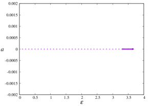
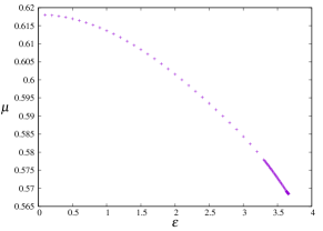
Figure 1. Continuation w.r.t. $\varepsilon$ of a non-$a$-twist circle with frequency $\omega$ (symmetric case): (left) adjusting parameter $a$; (right) unfolding parameter $\mu$.

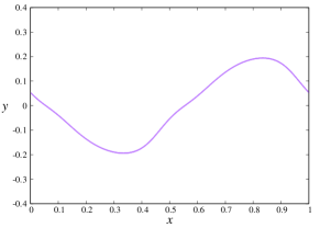
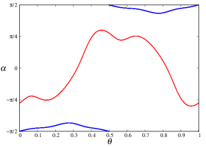
(a) $\varepsilon=2.000000$, $a=0.000000$, $\mu=0.6015602$

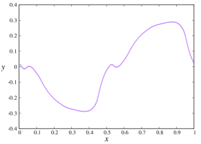
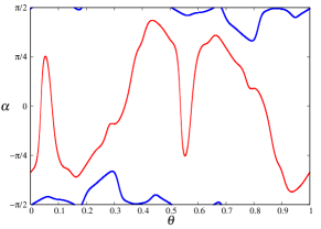
(b) $\varepsilon=3.000000$, $a=0.000000$, $\mu=0.5843217$

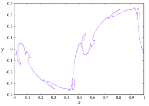
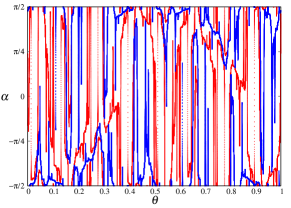
(c) $\varepsilon=3.658600$, $a=0.000000$, $\mu=0.5684363$

Figure 2. Continuation w.r.t. $\varepsilon$ of a non-$a$-twist circle with frequency $\omega$ (symmetric case): (left) invariant circle; (right) projectivized tangent bundle (in red) and stable bundle (in blue).

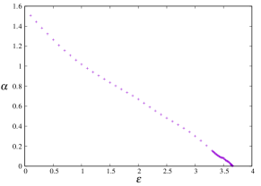
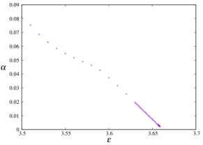
Figure 3. Continuation w.r.t. $\varepsilon$ of a non-$a$-twist circle with frequency $\omega$ (symmetric case): (left) minimum angle $\alpha$ between the stable and tangent bundles as function of $\varepsilon$; (right) critical behavior. The breakdown of the circle is produced at $\varepsilon_{\rm c}\simeq 3.662396$.

The symmetry properties of the family lead to several features. First, parameter $a$ is always $0$, as it is shown in Figure 1. Moreover, the non-$a$-twist circles and their bundles have also symmetry properties, as it is shown in Figure 2. In particular, We note that the collapse in this symmetric case happens on both sides of the bundles. We expect that when the bundles collapse, there will be no gap between the bundles on either side of the bundles with respect to $\alpha$. Later in this section, we will see that in the nonsymmetric the bundles collapse leaving a gap between the bundles for all values of $\theta$, but only on one side of the bundles with respect to $\alpha$.

We also performed some computations to illustrate that the analytic condition that the invariant circle is non-$a$-twist translates into dynamical properties of the rotation number of the invariant cicle when we move parameters. We implement the algorithm in Section 3.1 to continue invariant tori regardless the internal dynamics and compute the corresponding rotation number, by starting with a non-$a$-twist circle from the previous implementation. In particular, we have selected a non-$a$-twist circle for $\varepsilon=2.2$, so that $\mu=1.5984626393$ and $a=0$. We first perform continuations for $\mu$ and $\varepsilon$ fixed, increasing and decreasing the parameter $a$, respectively. The graph of the rotation number of the invariant circle as a function of $a$ is shown in Figure 4 (Left). As expected, the non-$a$-twist circle corresponds to a critical point of this graph. The graph is symmetric, also as expected from the symmetry properties of the family being studied. Notice also the presence of visible resonances, corresponding to rotation number $5/8$. However, by performing a continuation with respect to $\mu$ instead of $a$ (and starting with the same initial torus), we observe that the starting torus does not correspond to a minimum of the rotation number as a function of $\mu$, as shown in Figure 4 (Right). This is because the non-twist-property is associated to parameter $a$, and the invariant circle is $\mu$-twist.

Figure 4. Rotation number versus continuation parameter from the non-$a$-twist circle with $a=0.000000$, $\mu=0.5984626$, $\varepsilon=2.20000$ (symmetric case):
(left) continuation w.r.t. $a$; (right) continuation w.r.t. $\mu$.

4.3. Continuation of the non-$a$-twist circle in the nonsymmetric case

In this section we consider the family (31) with $p(x)=\tfrac{1}{2\pi}(\sin(2\pi x)+\cos(4\pi x)$, that (apparently) does not have symmetry properties. We again take $\sigma=0.8$, and $\omega=\tfrac{1}{2}(\sqrt{5}-1)$. We have followed the same plan as in previous example.

First, with algorithm of Section 3.2, we continue with respect to parameter $\varepsilon$ a non-$a$-twist circle with rotation number $\omega=\tfrac{1}{2}(\sqrt{5}-1)$. The adjusting parameters $a$ and $\mu$ as functions of perturbation parameter $\varepsilon$ are shown in Figure 5. Unlike the symmetric case, parameter $a$ varies, and remains bounded inside an interval of size $2.6\times 10^{-3}$ around zero. The continuation reaches the value $\varepsilon=1.230340$, in which the invariant circle is approximated with a truncated Fourier series with $524288$ modes. The process of breakdown and the collision of the invariant bundles is shown in Figure 6. We notice that in contrast with the bundle collapse in the symmetric version of the dissipative standard non-twist map, the collapse for this example only happens on one side of the bundles, leaving a gap between the bundles. The minimum angle between bundles is also asymptotically linear when close to breakdown, see Figure 7, from which we can extrapolate the critical value $\varepsilon_{\rm c}\simeq 1.240522$.

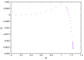
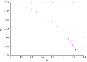
Figure 5. Continuation w.r.t. $\varepsilon$ of a non-$a$-twist circle with frequency $\omega$ (non-symmetric case): (left) adjusting parameter $a$; (left) unfolding parameter $\mu$.

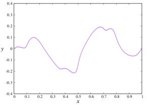
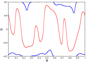
(a) $\varepsilon=1.000000$, $a=7.646104\cdot 10^{-4}$, $\mu=0.6031124$

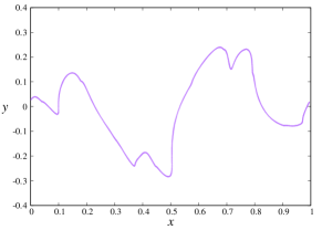
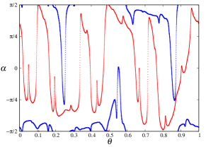
(b) $\varepsilon=1.200000$, $a=-9.571568\cdot 10^{-4}$, $\mu=0.5951423$

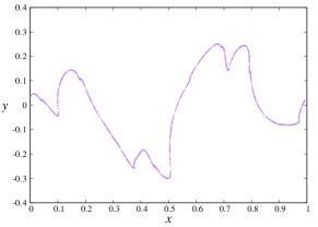
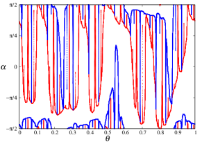
(c) $\varepsilon=1.240340$, $a=-2.588932\cdot 10^{-3}$, $\mu=0.5932114$

Figure 6. Continuation w.r.t. $\varepsilon$ of a non-$a$-twist circle with frequency $\omega$ (non-symmetric case): (left) invariant circle; (right) projectivized tangent bundle (in red) and stable bundle (in blue).

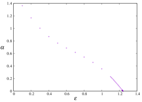
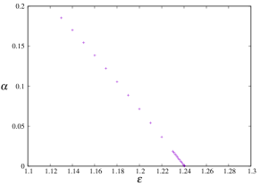
Figure 7. Continuation w.r.t. $\varepsilon$ of a non-$a$-twist circle with frequency $\omega$ (non-symmetric case): (left) minimum angle $\alpha$ between the stable and tangent bundles; (right) critical behavior. The breakdown of the circle is produced at $\varepsilon_{\rm c}\simeq 1.240522$.

As in the first example, in Figure 8 we show the graph of the rotation number of the invariant circle as a function of a parameter of continuation (either $a$ or $\mu$) starting at a non-$a$-twist circle for $\varepsilon=1.00000$, $a=7.646104\cdot 10^{-4}$, $\mu=0.6031124$. The figure provides again a dynamical interpretation of the fact that the invariant circle is non-$a$-twist, but $\mu$-twist.

Figure 8. Rotation number versus continuation parameter from the non-$a$-twist circle with $a=7.646104\cdot 10^{-4}$, $\mu=0.6031124$, $\varepsilon=1.00000$ (non-symmetric case): (left) Continuation w.r.t. $a$; (right) Continuation w.r.t. $\mu$.

In Figure 9, we show continuations with respect to $\varepsilon$ of invariant circles with fixed frequency $\omega$ and different values of the $a$-twist. That is, we compute the surface of parameter points for which there is an invariant circle with frequency $\omega$. We plotted this surface showing the values of $a$ and $\mu$ along the $\varepsilon$ continuation. In particular, the continuation curve corresponding to an $a$-twist $b_{a}$ starts with $a=\frac{1}{2}b_{a}$, $\mu=\omega-a^{2}$ and $\varepsilon=0$. We have highligted the curve corresponding to zero $a$-twist. Note that the surface is not symmetric with respect to $a$ and for negative $a$-twist there is a region where the circles seem to persist for larger values of $\mu$ and $\varepsilon$.

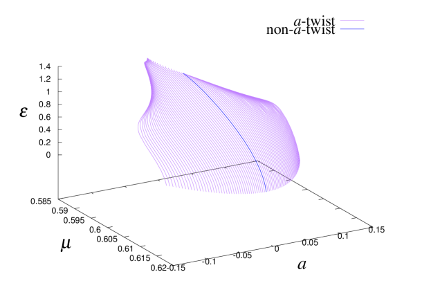
Figure 9. Parameter surface generated by continuation w.r.t. $\varepsilon$ of invariant circles with frequency $\omega$ and fix $a$-twist (non-symmetric case).

5. Conclusions

In this paper we have clarified the property of being non-twist for a circle, in the context of conformally symplectic systems. This non-twist property has to do with the degeneracy condition arising when tuning a particular parameter to fix the dynamics of an invariant circle to a given rotation number. Hence, the non-twist condition is with respect to a particular parameter. As such, the concept can be extended to many other systems in which parameters have to be adjusted to fix the frequency, as in [CH17a]. In symplectic systems, the parameters to adjust are the actions of a torus.

We have also presented several algorithms for computing invariant circles, including non-twist circles and a methodology to compute parametric surfaces in parameter space corresponding to invariant circles with a prescribed (Diophantine) frequency. The key of our methodology is introducing a concept of twist with respect to a parameter, so one can compute continuation curves corresponding to a fix twist. Unlike the symplectic case, non-twist tori in conformally symplectic systems do not seem to be the more robust, meaning they are not the ones that survive for greater values of perturbation parameters.

The algorithms are very efficient, and let us compute invariant circles even with hundreds of thousands of Fourier coefficients, and then explore the regimes at the verge of analyticity breakdown.

References

- [BHS96] H.W. Broer, G.B. Huitema, and M.B. Sevryuk, Quasi-periodic motions in families of dynamical systems. Order amidst chaos, Lecture Notes in Math., Vol 1645, Springer-Verlag, Berlin, 1996.
- [Can14] Marta Canadell, Computation of normally hyperbolic invariant manifolds, Ph.D. thesis, Universitat de Barcelona, Barcelona, Spain, June 2014.
- [CC10] Renato Calleja and Alessandra Celletti, Breakdown of invariant attractors for the dissipative standard map, Chaos 20 (2010), no. 1, 013121, 9. MR 2730168
- [CCdlL13] R. Calleja, A. Celletti, and R. de la Llave, A KAM theory for conformally symplectic systems: efficient algorithms and their validation, J. Differential Equations 255 (2013), no. 5, 978–1049.
- [CdlL09] R. Calleja and R. de la Llave, Fast numerical computation of quasi-periodic equilibrium states in 1D statistical mechanics, including twist maps, Nonlinearity 22 (2009), no. 6, 1311–1336.
- [CdlL10] Renato Calleja and Rafael de la Llave, Computation of the breakdown of analyticity in statistical mechanics models: numerical results and a renormalization group explanation, J. Stat. Phys. 141 (2010), no. 6, 940–951. MR 2740396
- [CF12] R. Calleja and J.-Ll. Figueras, Collision of invariant bundles of quasi-periodic attractors in the dissipative standard map, Chaos: An Interdisciplinary Journal of Nonlinear Science 22 (2012), no. 3, 033114.
- [CH14] M. Canadell and A. Haro, Parameterization method for computing quasi-periodic reducible normally hyperbolic invariant tori, F. Casas, V. Martínez (eds.), Advances in Differential Equations and Applications, SEMA SIMAI Springer Series, vol. 4, Springer, 2014.
- [CH17a] M. Canadell and À. Haro, Computation of Quasi-Periodic Normally Hyperbolic Invariant Tori: Algorithms, Numerical Explorations and Mechanisms of Breakdown, J. Nonlinear Sci. 27 (2017), no. 6, 1829–1868. MR 3713932
- [CH17b] by same author, Computation of Quasiperiodic Normally Hyperbolic Invariant Tori: Rigorous Results, J. Nonlinear Sci. 27 (2017), no. 6, 1869–1904. MR 3713933
- [dlLGJV05] R. de la Llave, A. González, À. Jorba, and J. Villanueva, KAM theory without action-angle variables, Nonlinearity 18 (2005), no. 2, 855–895.
- [FH15] Jordi-Lluís Figueras and Àlex Haro, Different scenarios for hyperbolicity breakdown in quasiperiodic area preserving twist maps, Chaos 25 (2015), no. 12, 123119, 16. MR 3436748
- [GHdlL14] A. González, A. Haro, and R. de la Llave, Singularity theory for non-twist KAM tori, Mem. Amer. Math. Soc. 227 (2014), no. 1067, vi+115.
- [Gra17] Albert Granados, Invariant manifolds and the parameterization method in coupled energy harvesting piezoelectric oscillators, Phys. D 351/352 (2017), 14–29. MR 3659393
- [HCF+16] À. Haro, M. Canadell, J.-Ll. Figueras, A. Luque, and J.-M. Mondelo, The parameterization method for invariant manifolds, Applied Mathematical Sciences, vol. 195, Springer, [Cham], 2016, From rigorous results to effective computations. MR 3467671
- [HdlL06] A. Haro and R. de la Llave, Manifolds on the verge of a hyperbolicity breakdown, Chaos 16 (2006), no. 1, 013120, 8.
- [HdlL07] by same author, A parameterization method for the computation of invariant tori and their whiskers in quasi-periodic maps: explorations and mechanisms for the breakdown of hyperbolicity, SIAM J. Appl. Dyn. Syst. 6 (2007), no. 1, 142–207 (electronic).
- [Mos66] J. Moser, A rapidly convergent iteration method and non-linear differential equations. II, Ann. Scuola Norm. Sup. Pisa (3) 20 (1966), 499–535.
- [Mos67] by same author, Convergent series expansions for quasi-periodic motions, Math. Ann. 169 (1967), 136–176.