Hardware-Accelerated SAR Simulation with NVIDIA-RTX Technology

Abstract

Synthetic Aperture Radar (SAR) is a critical sensing technology that is notably independent of the sensor-to-target distance and has numerous cross-cutting applications, e.g., target recognition, mapping, surveillance, oceanography, geology, forestry (biomass, deforestation), disaster monitoring (volcano eruptions, oil spills, flooding), and infrastructure tracking (urban growth, structure mapping). SAR uses a high-power antenna to illuminate target locations with electromagnetic radiation, e.g., 10GHz radio waves, and illuminated surface backscatter is sensed by the antenna which is then used to generate images of structures. Real SAR data is difficult and costly to produce and, for research, lacks a reliable source ground truth. Few SAR software simulators are available and even less are open source and can be validated. This article proposes a open source SAR simulator to compute phase histories for arbitrary 3D scenes using newly available ray-tracing hardware made available commercially through the NVIDIA’s RTX graphics cards series. The OptiX GPU ray tracing library for NVIDIA GPUs is used to calculate SAR phase histories at unprecedented computational speeds. The simulation results are validated against existing SAR simulation code for spotlight SAR illumination of point targets. The computational performance of this approach provides orders of magnitude speed increases over CPU simulation. An additional order of magnitude of GPU acceleration when simulations are run on RTX GPUs which include hardware specifically to accelerate OptiX ray tracing. The article describes the OptiX simulator structure, processing framework and calculations that afford execution on massively parallel GPU computation device. The shortcoming of the OptiX library’s restriction to single precision float representation is discussed and modifications of sensitive calculations are proposed to reduce truncation error thereby increasing the simulation accuracy under this constraint.

1 Introduction

Synthetic Aperture Radar (SAR) is an image formation process that uses pulses of electromagnetic radiation emitted and sensed by a high-power antenna from a moving platform [1]. Application of SAR includes target recognition [2], mapping difficult terrain area [3], ocean surveillance [4], geology (structural mapping, lithological mapping, mapping geomorphological features, mineral exploration, active fault mapping) [5], mapping forest cover and biomass [6].

SAR imaging uses small antenna to illuminate large swaths of ground from different antenna locations [7]. The transmitted electromagnetic wave propagates and interacts with matter or objects. Optical sensors, using visible light, can only function in the daytime and measure reflected solar light. These sensors lose their utility when the surveyed region is obstructed by weather such as cloud coverage. Fortunately, microwaves can operate in day or night in nearly all weather conditions because of its ability to penetrate through clouds and vegetation (depending on frequency). Penetration through the forest canopy or into the soil is greater with longer wavelengths. It also has minimal atmospheric effects with minimal sensitivity to structure and dielectric properties. The received reflected data can be processed into a ground image using various SAR signal processing algorithms [8]. Each pixel of a radar image represents a complex quantity of energy that was reflected back to the antenna. The magnitude of each pixel represents the intensity of the reflected signal.

There are substantial challenges associated with SAR simulation. The critical components of SAR sensing are vehicle pose/trajectory, antenna aperture, SAR signal processing system, electromagnetic interaction with matter, and scene geometry. The scene has to be constructed which often uses a polygonal representation (triangle mesh) that define the shape and reflectance properties. The antenna must be defined next to establish its placement within the ”scene” and must replicate signal responses that coincide with the region of the scene that would be observed by the antenna. The simulated EM waves must propagate into the scene and calculate how they refract, attenuate, and reflect off scene surfaces. The computational complexity of the problem grows significantly as scenes become more intricate, having millions of polygons to trace, and the number of EM wave bounces that wish to be preserved.

There are multiple high-investment barriers that make generation of real-world SAR data difficult. SAR antenna typically emit high power pulse signals that exceed FCC broadcast regulations and as such require licensing to operate. SAR pulse emission and echo sensing typically require unobstructed views for distances $>$ 5 km. This requirement restricts deployment to aerial platforms. Further, signal processing algorithms for SAR require high-precision and high data rate knowledge of the vehicle position and orientation which requires costly positioning and guidance, navigation and control software. The radio frequency hardware (RF signal conditioning and antenna) is often extremely expensive, contains sensitive and highly-specialized circuitry, computing hardware and RF antenna hardware. Hence, cost, licensure, equipment, personnel, training and expertise makes the total cost-to-own for SAR technology prohibitive in reality. All of these barriers for SAR signal generation motivate the creation of software systems that can simulate the SAR sensing context.

Collected SAR data is subject to numerous noise source including EM noice, position error, non-planar targets, and range curvature. These errors make ground truth difficult to establish and hinder theoretical validation of SAR models for EM propagation and backscatter computation. Availability of simulated data with ground truth or deliberately introduced noise allows theoretical validation of SAR signal process and image reconstruction algorithms. For this reason, simulation data is often the preferred choice in research and development communities due to its versatility and smaller cost relative to collected measured data. Simulation tools provide the opportunity to mimic the effects of any radar platform in any environment under any specified conditions so long as the simulator has been developed to respond to such conditions.

Our SAR simulation goals seek to support two applications. The first application uses synthetically generated SAR images to facilitate deep learning SAR research and bolster the machine learning community with the capacity to incorporate synthetic data methods [9, 10]. The second application is to provide high speed SAR simulation of raw radar signals for real-time simulation of SAR imagery.

This work transforms and extends current electromagnetic (EM) wave propagation simulation models for SAR image formation using a low-cost, massively parallel and hardware accelerated computing architecture provided by NVIDIA’s recent RTX series of GPUs [11] in an effort to accelerate SAR simulation capabilities.

2 Related Work

SAR simulation requires solutions to far-field Electro-Magnetic (EM) wave propagation equations. Fortunately, these equations can be solved for approximately by breaking the complete solution into two parts: (1) solving for the geometric propagation of EM waves through 3D space, termed geometrical optics, and (2) solving for the physical interactions between EM waves and scene surfaces, termed physical optics. Our review of current state-of-the-art discusses the dominant simulation theoretical model, current implementations of this model and how this article advances state-of-the-art in this domain.

From a theoretical standpoint, current approaches overwhelmingly adopt the Shooting and Bouncing Ray (SBR) method [12]. These methods use geometric optics to simulate surface scattering of incident EM waves. Geometric optics theory use linear rays to model the direction of wave propagation and attributes each ray with a packet of energy distributed within a cylindrical region about a 3D ray, referred to as a ray tube [13]. Ray tube simulation is the basis of all SAR simulation techniques described in this article and is the dominant computational model for calculating EM wave scattering from surfaces for the purposes of simulating SAR wave propagation and, more generally, the Radar Cross Section (RCS) of scattering surfaces.

From a technical standpoint, current SAR simulation implementations are very limited consisting of few commercial [14, 15, 16] and even less open-source [17, 18] implementations. Commercial implementations pose difficult problems for validation, improvement and extension and may also be unavailable for public use (governmental or military use) or prohibitive in cost. Open-source approaches have limited application as they do not solve major fundamental technical technical problems including the ray tracing component of simulation [18].

One example of a commercialized SAR simulator described in the literature is Xpatch [14]. Xpatch is a validated radar simulation software package used by industry and government to simulate SAR images. As mentioned previously, the Xpatch simulator uses 3D models and simulates EM waves using the Shooting and Bouncing Ray (SBR) method. Xpatch provides the user the ability to generate Radar Cross Section (RCS), High Resolution Range (HRR) profiles, and Synthetic Aperture Radar (SAR) imagery. Unfortunately, the tool is proprietary, therefore does not lend the option for open-source use.

The leading example of an open-source SAR simulator is RaySAR [19]. RaySAR uses custom modifications to the open source POV-Ray (Persistence Of Vision) ray tracing engine to model EM wave propagation, reflection and backscatter [20, 17]. RaySAR requires the user to employ the RaySAR-customized POV-Ray software to solve for geometric EM wave and surface intersection locations that track wave intensity and direction as the EM waves bounce across potentially multiple surface-to-surface reflection paths resulting in a (sometimes large) output data file. RaySAR’s main interface uses MATLAB to analyze the POV-Ray generated data file and compute the final simulation result. Shortcomings of this approach are: (1) MATLAB is required to run the simulator, (2) POV-Ray uses CPU ray tracing which can be slow and also generate very large data files for complex 3D scenes and (3) the simulator only uses ray traced solutions for a single view which makes the simulated reconstruction inaccurate; especially when the aperture is large.

In contrast to these approaches, we propose a completely new computational paradigm for solving the geometrical optics problem of SAR simulation.

1. Our proposed OptiX SAR simulator is open source and does not require third party programs, e.g., MATLAB.

2. Our proposed OptiX SAR simulator uses extremely fast GPU parallel processing to compute the ray traced solution.

3. Our proposed OptiX SAR simulator calculates ray traced solutions for multiple views making the simulated reconstruction accurate even when the aperture is large.

The cumulative impact of these contributions is a new SAR simulation framework that applies to most airborne SAR sensing contexts that can simulate SAR backscatter from complex 3D scenes at unprecedented performance rates.

3 Background

Our approach makes extensive use of the OptiX ray-tracing library to achieve unprecedented performance in calculating the geometric optical propagation for SAR simulation. In this section we provide a brief overview of the OptiX system and detail its unique massively-parallel execution structure. An understanding of this structure is crucial to the development of our proposed OptiX-based SAR simulation approach.

3.1 OptiX Ray-Tracing Engine

In this paper, we will utilize the OptiX library [21] from NVIDIA and special-purpose NVIDIA RTX GPU hardware to provide hardware-acceleration and enhancing computational speed for calculating ray tracing results for scenes having arbitrary 3D structure. RTX technology has been shown to successfully accelerate similar applications in computer graphics where deployment of RTX GPU-hardware acceleration [11] offers an increase of approximately $3.5X$ beyond non-RTX technology for real-time ray tracing.

OptiX [22] ray tracing engine has seven different types of programs, i.e, ray generation, intersection, closest hit, any hit, miss, exception and selector visit. In addition, a bounding box program operates on geometry to determine primitive bounds for accelerated structure construction. The core operation, rtTrace, alternates between locating an intersection (Traverse) and responding to that intersection (Shade). GPU support includes geometry acceleration and scenegraph (which can be dynamically modified). Also, GPU acceleration for custom intersection processing (shaders) includes a Miss program (rays that miss targets), Closest hit program (reflection, surface interactions) and Any hit program (shadows).

Figure 1 from S. Parker et al. [23] depicts the operating principles of massively parallel OptiX raytracing. 1(a) shows a hierarchical organization of objects that makeup the OptiX context. Of particular note are the geometry instances and material instances. Geometry instances denote collections of polygons (typically triangle meshes) which will interact with traced rays. The specific interactions of the geometry instances depends upon the materials attributed to the geometry, e.g., green diffuse bunny and grey ground plane. The OptiX engine decomposes geometry into local sub-groups using a Bounding Volume Hierarchy (BVH) [24] to accelerate the search for ray-geometry intersection locations.

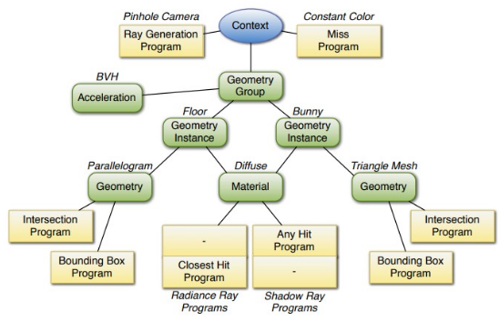
(a) Algorithm

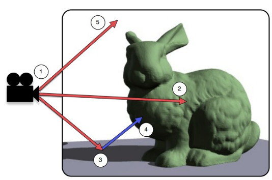
(b) Illustrated example

Figure 1: OptiX ray tracing of an example scene with a pinhole camera, two objects and shadows (a) algorithm (b) illustrated example (taken from [23]).

Figure 1(b) shows how rays are traced into a 3D scene by the OptiX engine. It depicts the five categories of rays that OptiX uses. To allow massively parallel raytracing, OptiX allows users to design small programs which can be associated with each ray category which are invoked as required to generate a raytracing result. Provided the example in Figure 1, the OptiX engine operates in the following fashion:

1. A ray generation program is a starting point for execution. This program creates and traces rays into the 3D scene. Each ray initiates a BVH traversal to determine how the ray interacts with geometries of the context.

2. A closest hit program will be called for those rays that intersect scene geometries. OptiX invokes the program and passes it the 3D intersection location and the local surface geometry which can be used to modify the ray tracing result or emit new rays.

3. A any hit program will be called when a ray intersects the scene multiple times which is useful for computation of surface shadows and surfaces having transmissive material properties, e.g., glass simulation.

4. A miss program will be called for those rays which do not intersect any scene geometries.

5. An exception program will be called when unexpected ray tracing circumstances are detected by the OptiX engine.

The OptiX library integrates these programs to a structure purposefully designed to minimize dependency between traced rays which, by design, produce high performance ray tracing results for potentially complex phenomenon. Performance gains are reaped via massively parallel computation of programs that run asynchronously and within limited memory to perform local atomic contributions to the final result.

4 Methodology/ Research Description

Our implementation of SAR simulation adopts the NVIDIA OptiX library to compute the solution to the geometric optics problem. We break the complete simulation problem into (5) main parts:

1. Load the virtual 3D world into a OptiX context and send it to the GPU compute device(s).

2. Initialize models of the vehicle trajectory, pulse signal waveform and radiation characteristics of the SAR antenna.

3. Simulate the emission of SAR EM pulse and sensed backscatter by the antenna.

4. Advance the vehicle to the next position within the trajectory.

5. Return to step (3) until the backscatter from all pulses has been calculated; then exit.

The models applied in this article rephrase existing SAR simulation models to enable massively parallel and hardware accelerated computation of the backscatter signal through the OptiX library and its hardware realization on NVIDIA RTX GPUs.

4.1 OptiX Simulation

The SAR simulation software contains two parts; simulate the scene and simulate a SAR system. A 3D scene must be generated and loaded onto the GPU device(s). The scene contains all the models used to generate a simulated environment. This comprises of all the objects, including the basic material properties of each object that the user wishes to generate a radar response from. The scene also contains a description of the radar system which characterizes the antenna and radar platform. An observation view is also established to provide the user an overall view of the entire simulation, allowing the user to simultaneously monitor the radar and scene simulations as desired. The most complex portion is the SAR simulation which outlines how the phase history will be simulated using ray tracing to complete the SAR simulation. An in-depth description of the OptiX simulation is provided in the following sections.

4.2 Creating a Virtual 3D World into a OptiX context

We define 3D scenes using YAML format files [25]. Our simulator parses the simulation YAML file to virtually construct the 3D scene. Virtual worlds for SAR simulation include at least one instance of each of the following (5) objects:

• One (or more) descriptions of 3D scene geometries.

• One (or more) descriptions of scene lights.

• One set of SAR antenna parameters.

• One set of SAR signal processing system parameters.

• One set of vehicle trajectory and aperture parameters.

There are a total of (8) different YAML objects for the simulator. Scene geometries and their reflectance are specified using a combination of (3) YAML objects. The ”mesh” and ”primitive” YAML objects specify object geometry and ”material” YAML objects specify reflectance properties for geometries. The ”light” and ”camera” YAML objects serve to illuminate and visualize the virtual 3D scene (in the observation window) respectively. Finally the ”antenna,” ”sarsystem,” and ”trajectory” YAML objects specify the antenna, signal processing system and vehicle trajectory and aperture parameters respectively. Since YAML files are plain text, users can easily modify and recombine simulation configurations to create complex SAR simulations of 3D scenes.

YAML Object	Properties
camera	pose, $(x,y)$ resolution (pixels), $(x,y)$ field of view (degrees)
	and projection type: {pinhole, orthographic}
primitive	pose, material, size and shape type: {plane, box, sphere, torus}
mesh	pose, material, size, filename and file format: {OBJ, PLY}
material	shader program: {diffuse, specular, specular-transmissive, phong},
	and reflectance parameters
light	pose, size, intensity, and light color
antenna	pose, intensity, size, shape, efficiency and type: {transceiver, transmitter, receiver}
sarsystem	carrier frequency (GHz), range resolution (m), range swath (m),
	number of frequencies, polarity type: {HH, HV, VH, VV}
trajectory	pose (as slant range (m) at point of closest approach and depression angle (deg))
	$(x,y,z)$ target position, Synthetic aperture size as Azimuth start and end (deg)
	Number of pulses, and SAR mode: {Linear Spotlight, Circular Spotlight, Stripmap}

Table 1: Simulation text file YAML objects and their parameters.

Each YAML object has a variety of options. Table 1 summarizes the properties of the YAML objects. The SAR antenna is specified by describing the operating bandwidth and the mode i.e. spotlight and stripmap. If we consider a scenario where the scene is stationary, the antenna has to traverse to generate simulated phase history data used for SAR image formation.

4.2.1 Describing and Visualizing the Virtual 3D Scene

Virtual 3D scenes are constructed by adding 3D geometries to the scene and attributing these geometries with reflectance attributes to determine their radar cross section. Each YAML file also includes camera and light objects to allow the 3D scene structure to be visualized using conventional ray tracing. The user can navigate the scene in this window to view and visually validate the structure of the simulated 3D scene.

A summary of the capabilities of the simulator for 3D scene creation and visualization are listed below:

• Camera - sets the observer view when the scene is shown in the interactive window

• Lights - lights required to view the scene as an observer

• Objects

  • Primitives - spheres, boxes, planes, torus and parallelogram

  • Mesh - we can load and place 3D mesh models into the 3D scene.

  • Materials - objects are attributed with materials to model how they reflect incident light and SAR radiation.

Our ray tracing method for visualization (and SAR simulation of) 3D scenes seek to compute pixel color and intensity by calculating the integral of the radiated energy incident to the surface of each pixel. To do so, we trace rays from each pixel into the 3D scene and, when intersections are found, we determine the amount of energy reflected onto each pixel in the (Red, Green, and Blue) spectrum. Calculation of the integral is computationally costly so an approximation that is both lower cost and compatible with parallel processing is provided by using Monte-Carlo/Metropolis integration. As shown in Figure 2(a), we perturb the origin of each traced ray which results in more accurate renderings of the simulated image. This technique is particularly suited for photon counting, i.e., energy tracking, rendering methods often used for photo-realistic ray tracing as in McGuire et al. [26]. Figure 2(b) shows a scene visualization using this approach that includes several 3D mesh objects: 2 tanks having blue diffuse reflectance, 1 box primitive also having blue diffuse reflectance, and 1 plane primitive having a green diffuse reflectance (the ground plane/background).

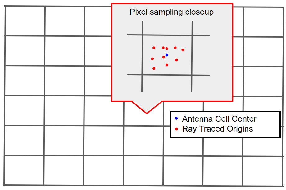
(a) pixel samping

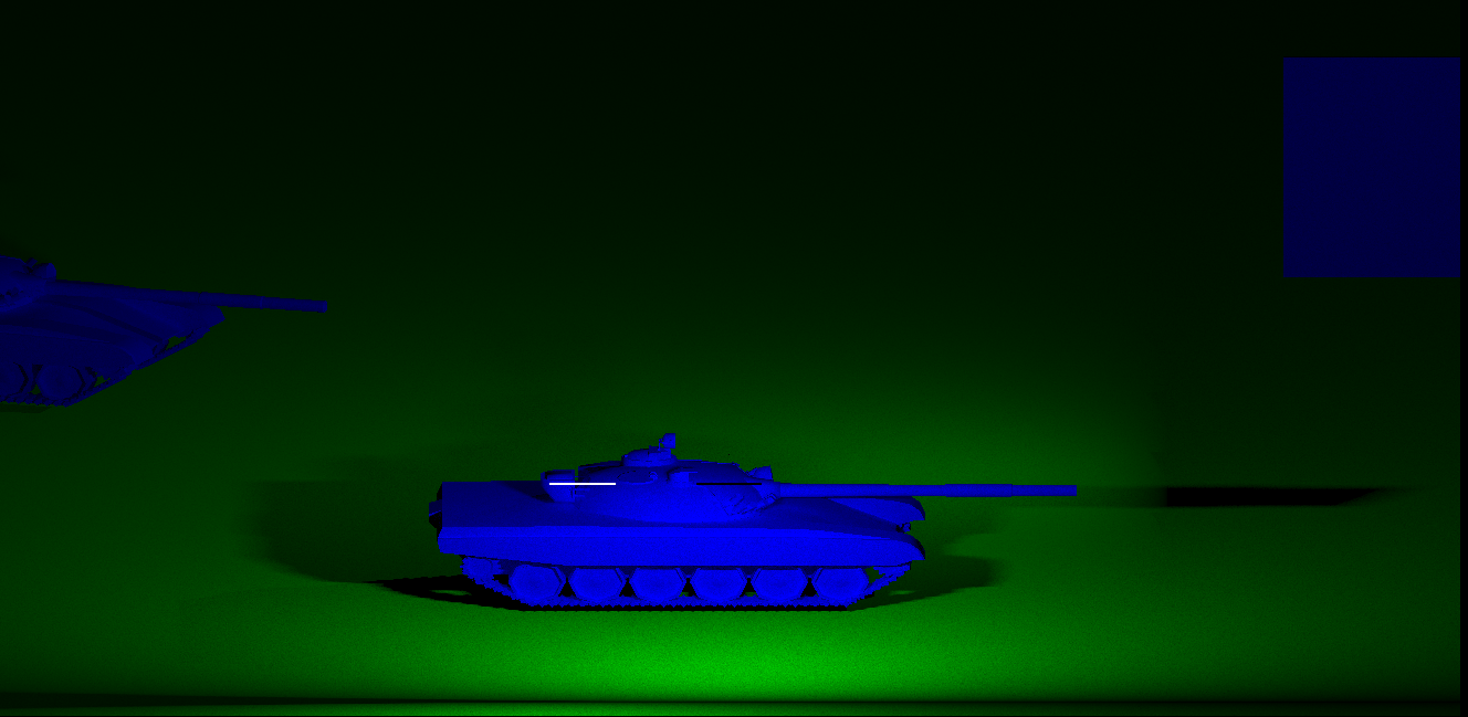
(b) A visualization of a SAR virtual world.

Figure 2: (a) shows details of pixel image formation via sampling the scene with perturbed ray origin positions within a pixel. (b) shows a visualization of a simple scene using these image formation principles.

4.2.2 Describing the SAR Emission and Sensing Process

A description of the virtual SAR sensing context is comprised of 3 parts: (1) a description of the SAR antenna, (2) a description of the SAR signal processing system and (3) a description of the vehicle trajectory.

The SAR antenna is considered to be mounted on the vehicle having the shape and dimensions specified by the antenna YAML object. We model the physical aperture of the antenna similar to that of the conventional camera as described in Figure 2(b). Yet, the field of view and resolution of the antenna cells are determined by the antenna radiation pattern. Our simulator assumes radiated energy out of the antenna aperture is sufficiently large only over the main lobe of the antenna radiation pattern. Hence, the field of view is taken as the angular span between the first pattern nulls adjacent to the main lobe, referred to as the “First Null Beam Width.” Simulation currently supports antenna or antenna arrays that can be modeled as a single rectangular patch. Depending upon the SAR measurement mode, the antenna will either remain static (stripmap SAR) or actuate as the vehicle moves (scanning, spotlight SAR). The antenna intensity parameter is used to distribute radiated energy across the aperture creating a unique energy for each aperture cell.

The SAR signal processing system characterizes the control timing and structural content of the signals radiated by the SAR antenna. This includes the polarity of the emitted and sensed radiation, each of which can be Horizontal (H) or Vertical (V) with respect to the antenna orientation generating four polarimetric modes: {HH, HV, VH and VV}. If nothing is specified, it takes the default value (sum all polarization states). Additional signal processing parameters specify the carrier frequency or operating frequency in GHz, the bandwidth of the emitted radiation specified as the desired range resolution and the discrete resolution of the sensed signal as the number of frequencies sensed in the return signal. The range resolution determines the bandwidth, i.e., range of frequencies emitted in each radiated SAR chirp pulse and determines the range resolution of the SAR system by descretizing the range swath into range cells as shown in Figure 3(b).

The vehicle trajectory is determined as a combination of the SAR mode and geometric positioning information. This information determines a collection of discrete locations from which the vehicle antenna emits pulses onto the target. The simulator allows four different SAR modes:

1. Spotlight (linear flight path with antenna and focal point movement),

2. Circular Spotlight (circular flight path with no antenna and focal point movement),

3. Scanning (linear flight path with antenna and focal point movement), and

4. Stripmap (linear flight path with no antenna and focal point movement).

Since all SAR modes have a common point of closest approach, this $(x,y,z)$ position determines the vehicle’s position at its midpoint in the aperture. This is taken as the unique $(x,y,z)$ point on the upper $(+z)$ hemisphere centered on the target point having radius $\rho_{s}$, azimuthal angle $\theta$, and depression angle $\psi$. The $(x,y,z)$ position is computed as a point in a spherical coordinate system having coordinates $(\rho_{s},\theta,\phi)$ where $\phi$ is the look angle, i.e., $\phi=\frac{\pi}{2}-\psi$. The azimuthal angle of closest approach is taken as the average of the aperture azimuth start and end angle, $(\theta_{s},\theta_{e})$, i.e., $\theta=\frac{\theta_{s}+\theta_{e}}{2}$. These parameters then jointly define a continuous model for the SAR vehicle trajectory. The number of pulses parameter, $N_{p}$, determines the sampling of this trajectory at discrete locations where pulses are spatially distributed over the aperture trajectory at equal intervals of arc-length for both linear or circular trajectories.

4.3 SAR Simulation

The second component to SAR simulation applies a model for EM wave propagation to calculate the sensed antenna signals for each pulse emitted from the antenna. SAR simulation is accomplished in the following sequence of steps:

1. Initialize the GPU device for SAR simulation and place the antenna at the required pose at the aperture start.

2. SAR pulse energy is distributed across a $N\times M$ grid of cells on the antenna aperture and OptiX ray tubes of descretized RF energy are traced into the 3D scene.

3. OptiX computes scene intersection locations and the “closest hit” program computes their contribution to SAR phase history for that pulse.

4. The vehicle is moved to the next location in the trajectory and returns to step (2) until the aperture end position is reached.

Once complete, the simulated backscatter sensed from RF energy reflected by scene surfaces is captured in the SAR phase history. This is the raw signal used by downstream reconstruction algorithms to calculate 2D SAR images of scene objects.

4.3.1 Intialization

The SAR simulation is initialized by attributing all scene objects with material properties that characterize their reflectance behavior for the chosen SAR frequency, e.g., X-band SAR uses 10GHz EM radiation. To preserve GPU device space and slightly improve performance, the observation window is made inactive and the lights of the virtual scene used for visualization are removed, e.g., “turned off,” to simplify the simulation.

A virtual antenna is created using the camera pixel model of Figure 2(a) to simulate the antenna aperture. Typically, for modestly large aperture antennae this produces a virtual camera view with a very long focal length due to the small field of view or, equivalently, small divergence, of the antenna beam intensity. The number of vertical pixels, or equivalently, range cells, is determined by the number of frequencies (range resolution) from the simulator settings. The antenna is placed such that it’s phase center is located at the vehicle trajectory starting position and oriented such that the plane of the patch antenna is perpendicular to the vector from the target position to the current vehicle position.

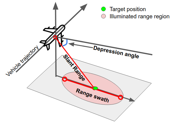
(a) SAR vehicle trajectory

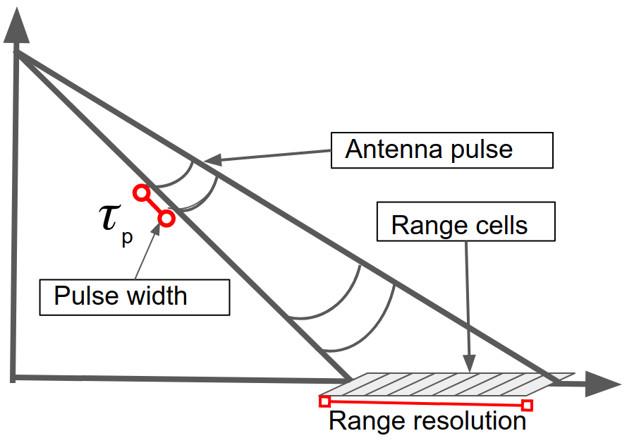
(b) SAR pulse and range resolution

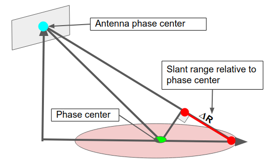
(c) SAR differential range

Figure 3: (a) shows the geometry of the SAR vehicle trajectory. (b) shows the parameters of the SAR signal pulses.

4.3.2 Theoretical Model: SAR Pulse and Phase History Simulation

We use the theoretical model of the Shooting and Bouncing Rays (SBR) method to calculate the backscatter sensed by the antenna in response to SAR pulses. The raw signal sensed by the antenna in response to a pulse is referred to as an echo. Each echo contains geometric and material information from the scene in the form of the scene backscatter encoded in space by the time-of-arrival of EM frequencies through observed magnitudes and phases of the emitted frequencies. Often this echo is represented by its Fourier transform, $S(f_{k})$. For the proposed OptiX simulator, there are $N_{p}$ pulses emitted from the vehicle as it traverses the synthetic aperture. Let $\tau_{i}$ denote the time at which the $i^{th}$ pulse is emitted with $i=1,2,\ldots N_{p}$. Using this notation we can construct a complex-valued 2D image $S(f_{k},\tau_{i})$ which is also referred to as the phase history. As such, the SAR simulation problem reduces to the problem of computing the phase history, $S(f_{k},\tau_{i})$.

To compute the phase history of a single pulse we must compute EM backscatter from the emitted antenna pulse. Assuming linearity, the total reflected energy is the sum of reflected energy from all illuminated surface positions. Note that, for planar surfaces, surface locations of constant (slant) range lie on hyperbolic curves and direct, i.e., round-trip antenna-surface-antenna, backscatter will arrive contemporaneously to the antenna and superimpose. To simplify the model, we eliminate the instantaneous position of the vehicle from the model by considering only the time-of-arrival relative to the target phase center, i.e., the middle of the range swath.

Let $(x,y,z)$ denote the 3D position of the antenna phase center and $p_{c}(\tau)=\left(x_{c}(\tau),\,y_{c}(\tau),\,z_{c}(\tau)\right){}^{T}$ denote the position of the target phase center at time $\tau$. Then slant range between the antenna phase center and target location is given by Equation (1).

$$d_{c}(\tau)=\sqrt{(x_{c}(\tau)-x)^{2}+(y_{c}(\tau)-y)^{2}+(z_{c}(\tau)-z)^{2}}$$ (1)

Let $p_{t}(\tau)=\left(x_{t}(\tau),\,y_{t}(\tau),\,z_{t}(\tau)\right){}^{T}$ denote an arbitrary third scene point, referred to as a target location, illuminated by SAR radiation. Similarly, the slant range between the antenna phase center and this target location is given by Equation (2).

$$d_{t}(\tau)=\sqrt{(x_{t}(\tau)-x)^{2}+(y_{t}(\tau)-y)^{2}+(z_{t}(\tau)-z)^{2}}$$ (2)

The differential range, $\Delta R(\tau)$, captures the difference in range (and sensed time of arrival at the antenna) between the target scene point and the phase center scene point as shown in Equation (3) and depicted in Figure 3(c).

$$\Delta R(\tau)=d_{t}(\tau)-d_{c}(\tau)$$ (3)

Using differential range, the SAR phase history output in the receiver from the arbitrary target location $p_{t}=(x,y,z)$ is given by Equation (4)

$$S(f_{k},\tau_{n})=A(f_{k},\tau_{n})\exp\left(\frac{-j4\pi f_{k}\Delta R(\tau_{n})}{c}\right)$$ (4)

where, pulse index, $\tau_{n}=(\tau_{1},\tau_{N_{p}})$, and frequency index, $f_{k}=(f_{1},f_{K})$. Unknown quantities that must be calculated via geometric optics include the geometric slant range between target scene locations and the antenna, $d_{t}(\tau)$ and the intensity of the reflection $A(f_{k},\tau_{n})$. Determination of $d_{t}(\tau)$ allows $\Delta R(\tau)$ to be computed and, by extension, the differential round-trip time of arrival between a target point reflection and a phase center point reflection. Note that this time difference can be made explicit via the substitution of this time difference as $\Delta t(\tau)=\frac{2\Delta R(\tau)}{c}$ in equation (4) where $2\Delta R(\tau)$ is the round trip differential distance. This substitution gives rise to the time-domain phase history signal shown in Equation (5).

$$S(f_{k},\tau_{n})=A(f_{k},\tau_{n})\exp\left(-j2\pi f_{k}\Delta t(\tau_{n})\right)$$ (5)

The target surface locations required to compute $d_{t}(\tau)$ across the region illuminated by the SAR antenna are determined by geometric ray tracing and the material reflectance properties which are attributed to each surface element to resolve the backscatter intensity $A(f_{k},\tau_{n})$. The OptiX simulator densely samples these intersection locations over the aperture of the antenna to compute the simulated SAR phase history.

4.3.3 NVIDIA OptiX Implementation: SAR Pulse and Phase History Simulation

OptiX is used to hardware-accelerate the calculation of 3D intersection locations of rays of electromagnetic radiation emitted into the scene. Figure 4 shows the OptiX SAR simulation processing blocks for single pulse phase history generation. The functional role of each block in Figure 4 is described in the following list:

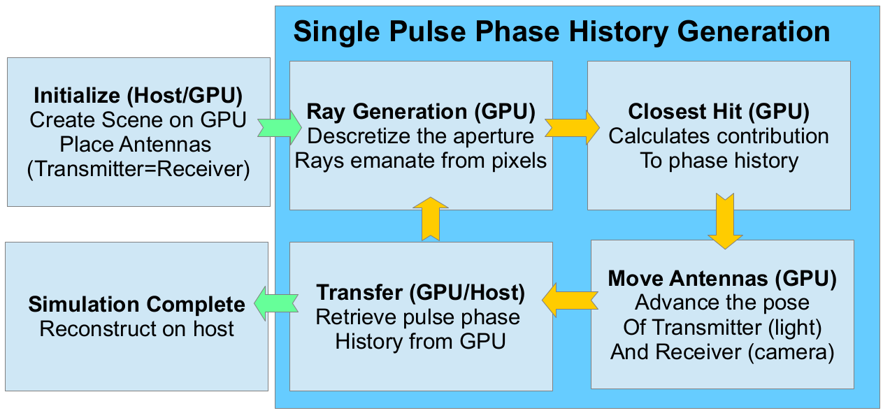
Figure 4: Current SAR simulation software using NVIDIA’s OptiX ray tracing computational framework

1. Initialize (Host & GPU): All parameter files and data are loaded from host storage and the 3D SAR simulation scene context is created on the GPU device.

2. Ray Generation (GPU): The ray generation program discretizes the aperture and traces a random ray from each pixel in the descretize antenna aperture. The OptiX framework constructs and maintains all rays being traced.

3. Closest Hit (GPU): The majority of the SAR pulse echo simulation occurs within this program. OptiX invokes the “closest hit” program for each ray that intersects a scene object. The scene intersection location and intensity of the incident ray are used to calculate the contribution of this target to the current pulse phase history equation (4).

4. Move Antennas (GPU): Once all rays for an antenna position have been traced, the antenna is moved to the next position in the trajectory and, if applicable, the antenna pose is updated. A new pulse phase history is simulated by returning to step (2) until all pulses have be integrated into the phase history, $S(f_{k},\tau_{n})$.

5. Transfer (GPU $\longrightarrow$ Host): The phase history values are transferred off the GPU device and back to the CPU host for storage and potential use in SAR image reconstruction algorithms.

The joint impact of these programs allows on-device hardware accelerated computation of simulated SAR EM pulse phase history. The developed OptiX program code is compatible with many NVIDIA devices allowing for simulation on most contemporary NVIDIA GPUs. Further, the code can utilize multiple GPUs to further accelerate calculation.

The ray generation step propagates EM waves into the scene and ray tracing continues as these rays reflect within the scence until all rays have either: (1) missed a surface or (2) been terminated. Ray termination occurs when the ray’s number of surface reflections, i.e., bounce levels, exceeds the user settings or if the ray energy decays below a threshold. Higher quality simulation may generate rays and accumulate the sensed echo multiple times which is common practice for ray tracing in computer graphics contexts.

Contributions to the phase history are computed within the “closest hit” program. Specifically, the “closest hit” program first uses the surface reflectance to determine the magnitude of energy reflected in the direction of the antenna. For surfaces having significant backscatter energy in the direction of the antenna, we compute the sensed magnitude, $A(f_{k},\tau_{n})$, and relative slant range, $\Delta R(\tau)$, from Equation (4) and add the appropriate contributions to phase history for each frequency. The location of the surface intersection provides $d_{t}(\tau)$ from which $\Delta R(\tau)$ can be computed giving a phase value $\psi(f_{k},\tau_{n})=j4\pi f_{k}\frac{\Delta R(\tau_{n})}{c}$. The magnitude, $A(f_{k},\tau_{n})$, is computed from the incident ray intensity and the local surface reflectance and apparent size of the antenna from the perspective of the surface (foreshortening). Rays with significant reflected energy in directions other than the antenna emit new rays in the reflected direction for “multi-bounce” ray simulation.

4.3.4 OptiX Simulation with Single Precision Float Calculations

One shortcoming of simulation using the OptiX ray tracing library is that all OptiX accelerated computations are restricted to use single precision float values. For SAR simulation this is a challenge due to the relative scale of the emitted EM frequency wavelengths and the distances over which these waves propagate in simulation to calculate the phase history.

Consider a simulation situation where an aerial vehicle at 10km slant range emits a X-band pulse of RF energy as a SAR RF pulse. Given that the wavelength of the emitted X-band frequencies are close to $3$cm, there is a significant difference in the relative size of the numbers in the phase calculation. More specifically, the phase calculation of equation (4) for frequency $f_{k}$ is given by $\psi(f_{k},\tau_{n})=j4\pi f_{k}\frac{\Delta R(\tau_{n})}{c}$. This calculation involves very large numbers, e.g., $c=0.299792458*10^{9}$ m/sec and $f_{k}$ having magnitude $10*10^{9}$, and much smaller numbers, e.g., $\Delta R(\tau_{n})$ which has a maximum size of the range swath width ($<10000$ m). Direct calculation of the ratios involving large and small numbers, e.g., $\frac{\Delta R(\tau_{n})}{c}$, leads to significant truncation error due to limitations in the representation accuracy of single precision float numbers. We limit truncation error by representing frequencies $f_{k}$ as frequency relative to the center frequency, $f_{c}$, e.g., $f_{k}=f_{c}+k\Delta f$ where $k$ is an integer ($k=-\frac{K-1}{2},\ldots,\frac{K-1}{2}$ for $K$ frequencies) and $\Delta f=\frac{B}{N_{f}-1}$ where $B$ denotes the pulse bandwidth. Substituting this into the equation for phase we get $\psi(f_{k},\tau_{n})=j4\pi(f_{c}+k\Delta f)\frac{\Delta R(\tau_{n})}{c}$. At this point we compute the constants ($\frac{f_{c}}{c}$, $\frac{\Delta f}{c}$) using double precision and include these as constants in our single precision phase calculation which is now factored as a constant term $\psi(f_{k},\tau_{n})=j4\pi\frac{f_{c}}{c}+\frac{\Delta f}{c}k\Delta R(\tau_{n})$ limiting the on-device calculation to $k\Delta R(\tau_{n})$ which can be multiplied by double precision values for ($\frac{f_{c}}{c}$, $\frac{\Delta f}{c}$) on the host.

5 Results

Our experimental results are provided by analyzing the output of the simulator along (3) distinct dimensions of performance:

1. Computational performance experiments evaluate the speed of the OptiX-accelerated ray tracing for SAR simulation.

2. Numerical performance experiments evaluate the accuracy of the computed phase history solution.

3. Reconstruction performance experiments evaluate the effect of numerical errors from (2) on the output of two SAR image reconstruction algorithms.

Analysis details trade-offs in terms of performance benefits and accuracy costs associated with SAR simulation using OptiX accelerated GPU programming. We use as a control the SAR simulator provided in [27] which simulates SAR in MATLAB including computation of the phase history for multiple point target reflectors and reconstruction of 2D SAR images using the matched filter and backprojection algorithms.

5.1 Computational Performance Results

Our evaluation of SAR simulation performance compares the ray tracing speed of the OptiX acclerated simulator against that of the MATLAB simulator. We then analyze the relative speed of 4 different NVIDIA GPUs ranging from inexpensive laptop GPUs (GeForce 940M), inexpensive desktop GPUs (Quadro P620), more expensive GPUs (Quadro M5000) and recently released NVIDIA RTX GPUs which perform both massively parallel and hardware-accelerated ray tracing. We then investigate the benefit of using multiple GPUs to distribute the computation of ray tracing results.

Our first computational performance experiment benchmarks the MATLAB vs. OptiX speed by duplicating the three point target SAR simulation discussed in the results of Gorham et. al [27]. Table 2 contains the performance results found for this simulation. It is not surprising to speedups in excess of 100,000 considering the MATLAB code is in an interpreted language (Java) and does not benefit from any acceleration.

Algorithm	Device	Rays traced/sec	Speed-up factor
Gorham et. al. [27]	CPU	156.38 rays/sec	-
SimSAR OptiX	RTX 2070 (GPU)	1.53 Mrays/sec	100,000 x

Table 2: Three point target simulation MATLAB CPU vs OptiX speed performance comparison.

We then perform the same simulation of the three point target SAR simulation on (4) different NVIDIA OptiX GPUs. Table 3 contains the number of primary, secondary and tertiary rays traced during the SAR simulation of the experimental scene. Primary rays are emitted as a SAR pulse and are generated by the ray generation program. Secondary and tertiary rays are generated when surfaces reflect emitted rays once or twice respectively. The tabulated results of this experiment are shown in Table 3. The most significant finding is an order of magnitude ($\sim$x10) increase in computational performance afforded by the hardware accelerated RTX technology.

Device	GeForce 940M	Quadro M5000	Quadro P620	RTX 2070
Number of frequencies	512	512	512	512
Number of pulses	128	128	128	128
Primary rays (Mrays)	4.43	7.05	6.26	45.93
1 bounce rays (Mrays)	4.45	8.16	7.37	54.71
2 bounce rays(Mrays)	2.39	2.84	2.22	15.98
Closesthit (Mrays)	3.03	5.60	1.67	61.95
Total traced rays (Mrays)	14.30	24.04	17.53	178.57
Total Time (sec)	141.462	140.794	146.403	116.572
Performance (Mrays/s)	0.10	0.17	0.12	1.53

Table 3: Contribution of closest hit program and various depths of ray generation program in total ray counts. for three point target.

Experiment 3 constructs a scene from simplistic primitive shapes as provided by the YAML “primitive” object and some sample 3D triangular mesh objects. These objects and the number of vertices and triangles required to specify the object geometries are contained in Table 4.

Primitive type	Vertices	Triangles
Plane	4	2
Box	24	12
Sphere	16290	32040
Torus	32761	64800
T72.obj (tank in figure 2(b))	11348	18064
box.obj	24	24

Table 4: Vertex and Polygon counts for experimental 3D scene objects.

Our third computational performance experiment constructs a 3D scene from two tank mesh objects and inserts additional primitives into the scene including a plane and a box primitive. This scene has $\sim$22k (22724) vertices and $\sim$36k (36142) triangles as indicated by Table 4. It is important to note that the computational difficulty of the ray tracing result depends strongly on the number of polygons and (through the BVH hierarchy) the geometric distribution of the polygons in terms of local clustering. For example, scenes consisting of many polygons are more computationally intensive than lower polygon count scenes and when these polygons are non-uniform in size and spatial distribution, the computational costs for ray tracing increase. Table 4 contains our observed computational performance for ray tracing simulation on an RTX 2070 GPU.

Target	Scene 2 (36k triangles)
Device	RTX 2070
Number of frequencies	512
Number of pulses	128
Number of Vertices	22724
Number of Triangles	36154
Primary rays (Mrays)	176.96
1 bounce rays (Mrays)	184.97
2 bounce rays(Mrays)	108.15
Closesthit (Mrays)	162.39
Total traced rays (Mrays)	632.47
Total Time (sec)	148.477
Performance (Mrays/s)	4.26

Table 5: Performance of the OptiX simulator for the scene shown in Figure 2(b) which contains $\sim$36k polygons.

In summary, our results indicate that very large computational benefits are gained through the use of the OptiX ray tracing framework for simulation. Further, results show that, for our experimental scene, NVIDIA RTX hardware-accelerated computation provides an additional order of magnitude of compute acceleration beyond other GPU software implementations of OptiX.

5.2 Phase History Numerical Accuracy Results

Our evaluation of SAR simulation numerical performance compares the values of the computed phase history of the OptiX accelerated simulator against that of the MATLAB simulator. This is accomplished by taking the difference between the complex numbers of the OptiX and MATLAB phase histories. Let $S_{G}(f_{k},\tau_{n})$ and $S_{O}(f_{k},\tau_{n})$ denote $K\times N_{p}$ phase history images formed by a SAR simulation using of $k=1,\ldots,K$ discrete range frequencies and $n=1,\ldots,N_{p}$ cross-range pulses. We then consider the average numerical errors per frequency (for each range cell) as shown in Equation (6) and per pulse (for each cross-range measurement) as shown in Equation (7) respectively.

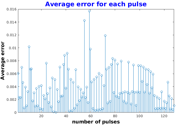
(a) Frequency (range cell) numerical error.

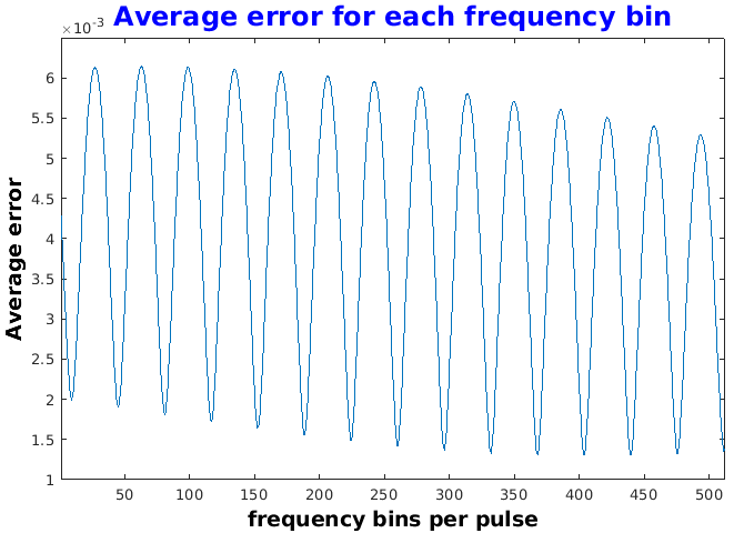
(b) Pulse (cross-range) numerical error.

Figure 5: (a,b) show numerical error between single precision OptiX SAR phase histories and double precision MATLAB phase histories. (a) plots the average numerical range cell error for a 512 frequency SAR simulation, $\epsilon_{f}(f_{k})$. (b) shows the average numerical cross-range cell error for a 128 pulse SAR simulation.

$$\epsilon_{f}(f_{k})=\frac{1}{N_{p}}\sum_{n=1}^{N_{p}}\left|S_{O}(f_{k},\tau_{n})-S_{G}(f_{k},\tau_{n})\right|$$ (6)

$$\epsilon_{\tau}(\tau_{n})=\frac{1}{K}\sum_{k=1}^{K}\left|S_{O}(f_{k},\tau_{n})-S_{G}(f_{k},\tau_{n})\right|$$ (7)

Results shown in Figure 5 show numerical errors. The numerical error is controlled by reorganizing the sensitive phase computation to re-express this calculation in terms of similar magnitude values to make full use of all available bits of precision in the single precision number format as described in § 4.3.4. The problem stems from the fact that single precision float number format has 24 precision bits. Accuracy in floating point multiplication for the number pair, $AB$, depends on the relative size of the two numbers. Specifically, large differences in the floating point exponent limits the accuracy of the calculated result. We maximize precision when these exponents are identical and, under these circumstances, the largest number of precision bits enter into the computed result. Identical exponents occur when the two numbers being multiplied are within a factor of two. The modification of § 4.3.4 achieves this goal by refactoring the phase calculation.

5.3 SAR Image Reconstruction Accuracy Results

Our evaluation of SAR simulation reconstruction performance compares the values of SAR images reconstructed from simulated phase history images provided by the OptiX acclerated simulator against that of the MATLAB simulator. Our results compare reconstruction results using two SAR image formation algorithms: (1) the matched filter algorithm and (2) the backprojection algorithm.

5.3.1 Matched Filtering and Backprojection Reconstruction Algorithms

SAR image formation from matched filtering is an optimal method to reconstruct the spatial $(x,y)$ reflectance of scene targets. It uses optimal detection theory to extract the known frequency responses present in the phase history and provides the maximum signal to noise ratio (SNR) image reconstruction assuming the phase history is perturbed by Gaussian noise. Matched filter reconstruction tailors a frequency-specific filter that will ideally match to the target. The matched filter response for target $p_{t}$ can be calculated using Equation (8) [27],

$$I_{mf}(p_{t})=\frac{1}{N_{p}K}\sum_{n=1}^{N_{p}}\sum_{k=1}^{K}S(f_{k},\tau_{n})\exp\left(\frac{j4\pi f_{k}\Delta R(\tau_{n})}{c}\right)=A_{0}$$ (8)

SAR image formation from the backprojection algorithm uses the theory of the inverse Radon transform to reconstruct the spatial $(x,y)$ reflectance of scene targets. Equation (9) details the computation required to calculate the backprojection response for target $p_{t}$.

$$I(p_{t})=\sum_{n=1}^{N_{p}}s_{int}(p_{t},\tau_{n})$$ (9)

where, $s_{int}(p_{t},\tau_{n})$ are values that are interpolated from the range profile, $s(m,\tau_{n})$. Equation (10) is the “range profile” value taken from the phase history at range bin $m$ and pulse $\tau_{n}$ , collected by $N_{p}$ pulses over a range of $K$ frequencies, is

$$s(m,\tau_{n})=\sum_{k=1}^{K}S(f_{k},\tau_{n})\exp\left(\frac{j4\pi f_{k}\Delta R(m,\tau_{n})}{c}\right)$$ (10)

After substituting $f_{k}=(k-1)\Delta f+f_{0}$ in the above equation and performing some algebric manipulation, Equation (10) can be expressed in terms of the inverse discrete Fourier transform as shown in Equation (11) [27].

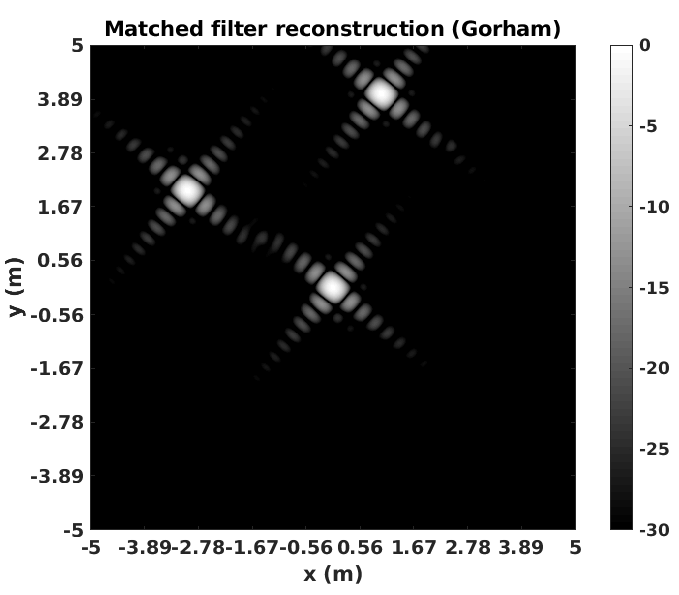
(a) MATLAB

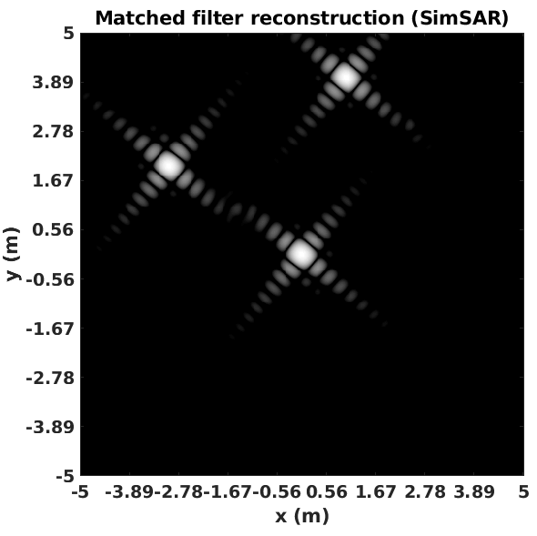
(b) OptiX simulator

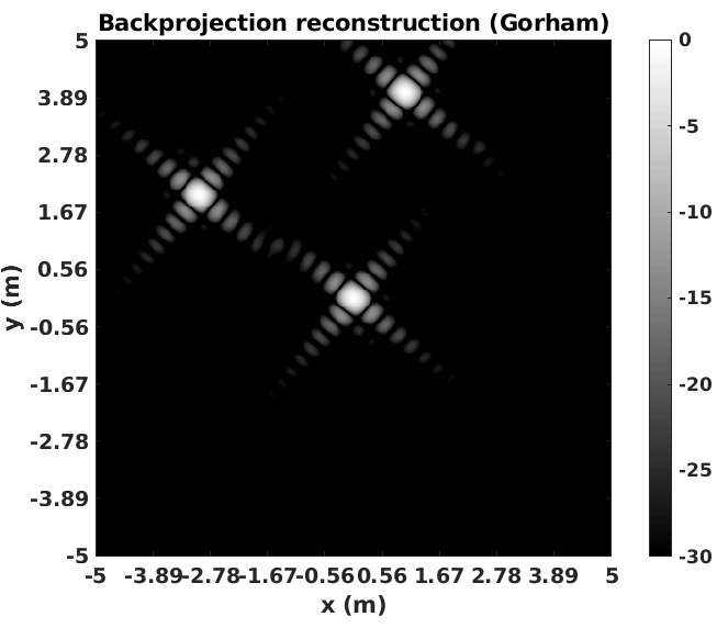
(c) MATLAB

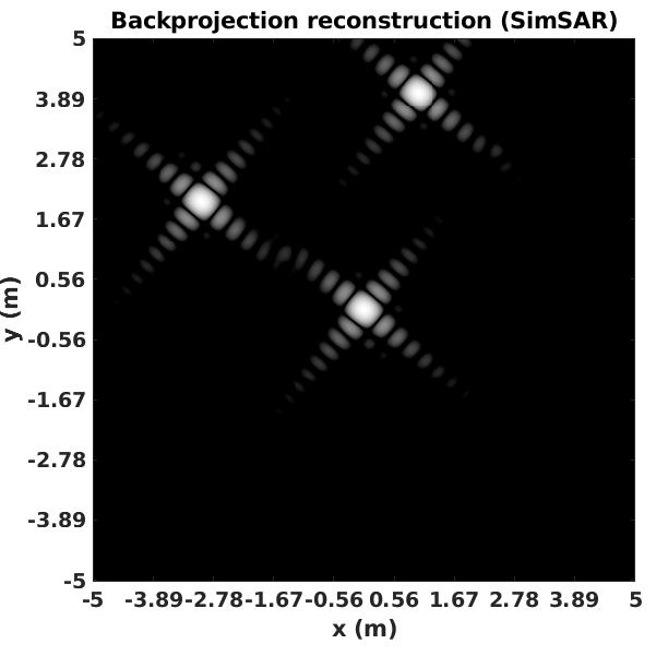
(d) OptiX simulator

Figure 6: (a,b) show MATLAB[27] and OptiX simulator SAR image reconstructions for 3 point targets using the matched filter algorithm. (c,d) show MATLAB and OptiX simulator SAR image reconstructions for 3 point targets using back projection algorithm.

$$s(m,\tau_{n})=N_{p}\cdot\{FT^{-1}(S(f_{k},\tau_{n}))\}\exp\left(\frac{j2\pi f_{1}(m-1)}{N_{p}\Delta f}\right)$$ (11)

Computation of the backprojection image is less computationally costly than matched filtering with a computational complexity of $O(N^{3})$. The backprojection algorithm can also take advantage of parallel processing and can be implemented on graphics processing units (GPU) [28, 29].

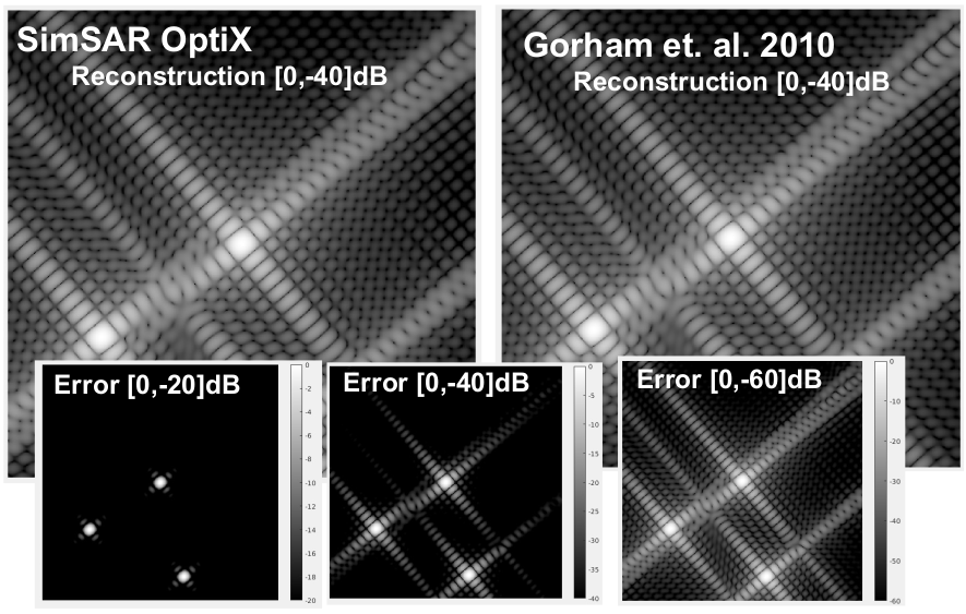
Figure 7: Numerical validation by forming a SAR image of a 3-point test target located having 3D locations (0,0,0), (-3,2,0), and (1,4,0). (left) shows OptiX accelerated simulation results. (right) shows results from Gorham et. a l. [27]. Bottom figures show three images highlighting small ($<$0.1 percent) numerical differences in the reconstructed SAR image values.

5.3.2 Reconstruction accuracy results

Figure 6 (a-d) shows SAR images formed for the 3 point target simulation duplicated from Gorham et. al. Phase history data was simulated for 3 point targets using Equation 4 where $A(f_{k},\tau_{n})$ = 1. Similar to Gorham et. al., $N_{p}$ = 128 pulses were simulated with $K$ = 512 frequency samples per pulse, a center frequency of 10 GHz and a 600 MHz bandwidth. A circular flight path was used with a 30 degree depression angle and a slant range of 10 km. A 3 degree integration angle was used with a center azimuth angle of 50 degrees. The scene extent was 10 m x 10 m with 2 cm pixel spacing in each dimension. We defined all the above parameters in an YAML file.

Figure 6(a,b) shows matched filter reconstructions and Figure 6(c,d) shows backprojection algorithm reconstructions for the OptiX simulator and the MATLAB simulator from Gorham et. al. While the images shown in this figure look very similar, one would suspect they are numerically distinct given the results of § 5.2.

Finally, Figure 7 shows both the reconstructed SAR images and the differences between the reconstructed images. Under this analysis we are able to see that, as one would suspect, larger errors in reconstruction occur in the vicinity of high-reflectance spatial locations.

6 Conclusion

This article proposes a Shooting and Bouncing Ray (SBR) approach for SAR simulation using NVIDIA’s OptiX library to accelerate the computationally expensive ray tracing calculations required by this approach. The computational performance of this approach provides orders of magnitude speed increases over CPU simulation and even more when using RTX graphics cards for simulation which can further accelerate the GPU calculations by a factor of 10 using ray tracing specific hardware. The new structure, processing framework and calculations required by the OptiX ray tracing library are described that allow the simulation software to run using one or more massively parallel GPU computation devices to obtain solutions to the geometric optics simulation at unprecedented speeds. The shortcoming of the OptiX library’s restriction to single precision float representation is discussed and modifications of sensitive calculations are proposed to reduce truncation error thereby increasing the simulation accuracy under this constraint. Computational performance is validated against one of the few open source SAR simulators available and demonstrate massive speed increases. Analysis is also made on the errors associated with simulation using single precision floats versus double precision floats and the impact of this restriction in accuracy is analyzed in both the calculation of the simulated phase history and for the reconstruction of the SAR spatial reconstruction images.

References

- [1] C. Wolff, https://www.radartutorial.eu/20.airborne/ab07.en.html, November 1999.
- [2] S. Chen and H. Wang, “SAR target recognition based on deep learning,” in 2014 International Conference on Data Science and Advanced Analytics (DSAA), pp. 541–547, 2014.
- [3] J. Zhang, S. Yang, Z. Zhao, and G. Huang, “SAR mapping technology and its application in difficulty terrain area,” in 2010 IEEE International Geoscience and Remote Sensing Symposium, pp. 3608–3611, 2010.
- [4] M. Yeremy, J. Campbell, K. Mattar, and T. Potter, “Ocean surveillance with polarimetric sar,” Canadian Journal of Remote Sensing 27(4), pp. 328–344, 2001.
- [5] Z. Perski, “Application of SAR imagery and SAR interferometry in digital geological cartography,” in The Current Role of Geological Mapping in Geosciences, S. R. Ostaficzuk, ed., pp. 225–244, Springer Netherlands, (Dordrecht), 2005.
- [6] A. Pulella, R. Aragão Santos, F. Sica, P. Posovszky, and P. Rizzoli, “Multi-temporal sentinel-1 backscatter and coherence for rainforest mapping,” Remote Sensing 12(5), 2020.
- [7] G. Charvat, J. Williams, A. Fenn, S. Kogon, and J. Herd, RES.LL-003 Build a Small Radar System Capable of Sensing Range, Doppler, and Synthetic Aperture Radar Imaging, January 2011.
- [8] W. Carrara, Spotlight synthetic aperture radar : signal processing algorithms, Artech House, Boston, 1995.
- [9] J. Cho, K. Lee, E. Shin, G. Choy, and S. Do, “How much data is needed to train a medical image deep learning system to achieve necessary high accuracy?,” Nov. 2015.
- [10] J. Tremblay, A. Prakash, D. Acuna, M. Brophy, V. Jampani, C. Anil, T. To, E. Cameracci, S. Boochoon, and S. Birchfield, “Training deep networks with synthetic data: Bridging the reality gap by domain randomization,” in The IEEE Conference on Computer Vision and Pattern Recognition (CVPR) Workshops, June 2018.
- [11] P. Andersson, J. Nilsson, M. Salvi, J. B. Spjut, and T. Akenine-Möller, “Temporally Dense Ray Tracing,” in High-Performance Graphics 2019 - Short Papers, Strasbourg, France, July 8-10, 2019, pp. 33–38, 2019.
- [12] H. Ling, R. . Chou, and S. . Lee, “Shooting and bouncing rays: calculating the RCS of an arbitrarily shaped cavity,” IEEE Transactions on Antennas and Propagation 37(2), pp. 194–205, 1989.
- [13] S. W. Lee, H. Ling, and R. Chou, “Ray-tube integration in shooting and bouncing ray method,” Microwave and Optical Technology Letters 1(8), pp. 286–289, 1988.
- [14] D. J. Andersh, J. Moore, S. Kosanovich, D. B. Kapp, R. Bhalla, R. Kipp, T. Courtney, A. Nolan, F. German, J. Cook, and J. Hughes, “Xpatch 4: the next generation in high frequency electromagnetic modeling and simulation software,” 2000.
- [15] JRM Technologies, OSV Radar, 2019.
- [16] Raytheon Corporation, “Raytheon inc., technology today: Highlighting raytheon’s technology,” pp. 34–35, 2013.
- [17] S. J. Auer, 3D Synthetic Aperture Radar Simulation for Interpreting Complex Urban Reflection Scenarios. Dissertation, Technische Universität München, München, 2011.
- [18] X. Wei-jie, L. W. Hua, W. P. Fei, L. Hai-lin, and Z. Jin-dong, “Sar image simulation for urban structures based on sbr,” 2014.
- [19] S. Auer, R. Bamler, and P. Reinartz, “RaySAR - 3D SAR simulator: Now open source,” in 2016 IEEE International Geoscience and Remote Sensing Symposium (IGARSS), pp. 6730–6733, July 2016.
- [20] S. Auer, S. Hinz, and R. Bamler, “Ray-tracing simulation techniques for understanding high-resolution sar images,” IEEE transactions on geoscience and remote sensing a publication of the IEEE Geoscience and Remote Sensing Society. 48(3), pp. 1445,1456, 2010-03.
- [21] NVIDIA Corporation, NVIDIA RTX platform, 2018.
- [22] NVIDIA Corporation, NVIDIA OptiX Ray Tracing Engine, 2018.
- [23] S. G. Parker, J. Bigler, A. Dietrich, H. Friedrich, J. Hoberock, D. Luebke, D. McAllister, M. McGuire, K. Morley, A. Robison, and M. Stich, “Optix: A general purpose ray tracing engine,” ACM Trans. Graph. 29, July 2010.
- [24] Y. Gu, Y. He, K. Fatahalian, and G. Blelloch, “Efficient BVH construction via approximate agglomerative clustering,” in Proceedings of the 5th High-Performance Graphics Conference, HPG ’13, p. 81–88, Association for Computing Machinery, (New York, NY, USA), 2013.
- [25] O. Ben-Kiki, C. Evans, and I. döt Net, “YAML ain’t markup language (YAML™) version 1.2,” 2001.
- [26] M. McGuire and D. Luebke, “Hardware-accelerated global illumination by image space photon mapping,” in ACM SIGGRAPH/EuroGraphics High Performance Graphics 2009, ACM, (New York, NY, USA), August 2009. Proceedings of the 2009 ACM SIGGRAPH/EuroGraphics conference on High Performance Graphics.
- [27] L. A. Gorham and L. J. Moore, “SAR image formation toolbox for MATLAB,” in Defense + Commercial Sensing, 2010.
- [28] T. Hartley, A. Fasih, C. Berdanier, F. Ozguner, and U. Catalyurek, “Investigating the use of GPU-accelerated nodes for SAR image formation,” pp. 1 – 8, 10 2009.
- [29] A. Rogan and R. Carande, “Improving the fast back projection algorithm through massive parallelizations,” in Radar Sensor Technology XIV, K. I. Ranney and A. W. Doerry, eds., 7669, pp. 144 – 151, International Society for Optics and Photonics, SPIE, 2010.