Mmwave Beam Management in
Urban Vehicular Networks

Abstract

Millimeter-wave (mmwave) communication represents a potential solution to capacity shortage in vehicular networks. However, effective beam alignment between senders and receivers requires accurate knowledge of the vehicles’ position for fast beam steering, which is often impractical to obtain in real time. We address this problem by leveraging the traffic signals regulating vehicular mobility: as an example, we may coordinate beams with red traffic lights, as they correspond to higher vehicle densities and lower speeds. To evaluate our intuition, we propose a tractable, yet accurate, mmwave communication model accounting for both the distance and the heading of vehicles being served. Using such a model, we optimize the beam design and define a low-complexity, heuristic strategy. For increased realism, we consider as reference scenario a large-scale, real-world mobility trace of vehicles in Luxembourg. The results show that our approach closely matches the optimum and always outperforms static beam design based on road topology alone. Remarkably, it also yields better performance than solutions based on real-time mobility information.

I Introduction

High-definition maps, their real-time updates, and on-board multimedia systems are just a few of the applications that make automated vehicles prime consumers of network traffic. Indeed, automotive services – both safety and entertainment – are among the reference use cases for next-generation network technologies, such as C-V2X  [1] and 802.11p/ITS-G5 [2]. In spite of the important differences among these technologies, they all share the goal of providing more network capacity to vehicles and drivers.

Whenever more capacity is needed, millimeter-wave (mmwave) communications are an appealing option [3]. On the negative side, mmwave frequencies suffer from harsh propagation conditions, with severe attenuation and high blockage probability. Such severe shortcoming has been addressed mainly by two approaches. On the one hand, mobile network operators plan to backup data transfers served by mmwave links by pairing them with lower-frequency links especially to maintain connectivity through low-frequency control channels, so as to cope with the unpredictable changes in real-world scenarios and the high sensitivity of mmwave to the presence of obstacles [4, 5]. On the other hand, the design of directional antenna systems, where the available power is concentrated on one or more beams, can significantly help to mitigate the problem[6]. An important trade-off in mmwave communications therefore arises between the directionality gain that can be achieved using beamforming and the spatial coverage that can be offered.

This implies that the performance of mmwave networks critically depends on the beam design, i.e., the number, direction, and amplitude of the beams. Successful beam design requires knowledge about the location of the user(s) to serve, which explains why the earliest and currently, the most mature, mmwave applications target static or quasi-static scenarios. In addition, due to the mobility of the vehicular users, communication in mmwaves is even more sensitive to high Doppler shift and delays in channel status feedbacks [7], which further complicates the beam training and design phases.

We address the above issues by leveraging the fact that, in urban environments, it is possible to acquire a great deal of information about vehicular mobility without detecting it in real time.

Consider, for example, the commonly observed situation that red traffic lights are associated with a higher vehicle density and lower speeds, two factors that can improve the achievable system throughput. This is very valuable information, and is known a priori. By exploiting this readily available information as well as static information such as road topology, we can facilitate efficient beam management without the need to make real-time decisions. Our high-level goal is to assess the performance of this approach, i.e., using traffic signal state information to complement and replace real-time mobility data. To our knowledge, this is the first work that optimizes beam design and carefully models mmwave coverage in vehicular networks, leveraging both road topology and traffic regulation signal information. In summary, we make the following main contributions:

• we first propose low-complexity approximations of the channel and beamforming behavior, tailored using empirical results obtained through real-world traces and show their excellent agreement with existing, more complex, models. Importantly, the applicability of our contribution goes beyond the scenario we study in this work;

• we formulate beam configuration as an optimization problem, aiming at maximizing the quality of coverage of vehicular users, i.e., the users’ sum rate. The choice of this objective, over others such as fairness or energy efficiency, reflects real-world operational scenarios where, as mentioned, it is foreseen that mmwave links are paired with low-frequency ones to ensure seamless connectivity. Thus, a sensible choice is to maximize not the number of mmwave links, but the number of high-quality ones;

• in light of the problem complexity, we define three alternative beam design strategies, among which we propose a low-complexity scheme, named Traffic Light (TL). Our scheme leverages road topology information and traffic light signals to efficiently configure the beams of the mmwave base stations;

• we show that TL closely matches the optimum, in terms of sum rate, in a small-scale scenario. Then we evaluate all of the above strategies using the large-scale trace representing the real-world topology and vehicular mobility of Luxembourg City. Our results show that, notwithstanding its much lower complexity, TL yields a performance comparable to that of solutions based on real-time mobility information.

In the following, we first discuss related work in Sec. II and detail the proposed system and mmwave communication models in Sec. III. Through numerical simulations and real-world vehicular traces, Sec. IV presents an accurate and scalable statistical model for the channel gain.

Sec. V introduces the proposed optimization problem and the beam management strategies we envision, while Sec. VI shows some results. Finally, Sec. VII concludes the paper.

II Related Work

Frameworks on how to model and analyze mmwave cellular networks have been provided in [8, 9], while channel characterization and modeling can be found in [10, 11].

These are statistical spatial models, based on experimental measurements, that accurately describe the mmwave channel, at a cost of a high complexity. Generalized, simpler models for the channel small-scale coefficients, as well as beamforming gains, can be found, e.g., in [6, 8]. Therein, the authors assume that small-scale channel gains are subject to Nakagami fading (i.e., a general model, encompassing Rayleigh distribution, that better suits mmwave propagation), while beamforming gains are modeled as discrete random variables with a probability mass function determined by the beamwidths of the transmitter and receiver beams.

More related to our study is the recent work in [12], which approximates the composite effects of the channel and beamforming gains, obtained under the models in [10], while also considering realistic antenna radiation patterns. Compared to this work, we additionally obtain the approximation of the channel and beamforming gains under the channel model adopted by 3GPP [11] and, more importantly, we differentiate between several levels of beam misalignment.

Beam training is another important challenge in mmwave-based mobile networks, including vehicular ones, mainly due to the associated control overhead and delay [3, 13]. In [14], the authors look at exhaustive and iterative search procedures, and further propose a two-stage hybrid training technique, in which the base station trains in the first stage and the user equipment performs reverse training in the second stage. In [15], the authors propose a framework that combines matching theory and swarm intelligence to dynamically and efficiently perform user association and beam alignment in a vehicle-to-vehicle (V2V) network.

Other popular approaches, more similar to the approach taken in this work, are predicated on hoarding and leveraging as much location information as possible, coming from the road-side sensors and the vehicles themselves [3, 16, 17], as well as from out-of-band direction interference [18]. In particular, using information originating from infrastructure nodes is the key to beam design and switching in [19, 20]. An inverse multipath fingerprinting approach is instead proposed in [21], with the aim to match potential beam directions with a vehicle location. Since collecting the information, processing it, and re-aligning the beams in near-real-time is a very challenging task, some works, e.g., [22], envision dispensing with beam realignment altogether, statically setting the beam orientation using road topology information.

Novelty. In addition to optimizing beam design, this study also assesses the viability and performance of TL, the low complexity scheme we propose. Importantly this study compares TL to the optimal configuration and other beam design strategies. To our knowledge, this is the first work that uses a combination of road topology and traffic signal information, both of which can be obtained beforehand, to enable and facilitate beam management decision-making in vehicular networks. It should be noted that all of the above mentioned works focus on beam aligning for each gNB-user pair, implicitly assuming that each narrow beam is employed to transmit to a single user only. However, in ultra dense scenarios, it is highly likely that even a beam as narrow as $5^{\circ}$ can cover several users simultaneously, users that can be multiplexed within the same beam. Thus, instead of focusing on perfectly aligning beams for each gNB-user pair, we look at how to align the beams at the gNB so as to maximize the quality of coverage of vehicles, i.e., the users’ sum rate. In addition, we argue that we can achieve such solutions while minimizing the use of real-time information, by utilizing instead, readily available, permanent, and deterministic information such as road topology and traffic light signals.

Finally, we would like to mention that a preliminary version of this work has been presented in our conference paper [23].

III Mmwave Vehicular Communication System

In this section, we introduce the model of the vehicular network and we provide details on the physical layer model that we adopt. We describe the signals transmitted by the mmwave base stations (hereinafter referred to as gNBs) and received by the vehicle, and we specify how beams are generated by the antennas.

TABLE I: Notation used in the system and communication model

Symbol	Type	Meaning
$\mathcal{G}$	set	Set of gNBs
$\mathcal{B}$	set	Set of beams; the generic element is denoted by $b$
$\mathcal{V}$	set	Set of vehicles; the generic element is denoted by $v$
$\mathcal{K}$	set	Set of time intervals; the generic element is denoted by $k$
$P_{tot}(g)$	parameter	Total power budget for gNB $g$
$N(g)$	parameter	Maximum number of beams for gNB $g$
$N_{t}$ ($N_{r}$)	parameter	Number of antenna elements per beam, at the transmitter (receiver) side
${\bf H}_{c}(g,v,k)$	parameter	Channel matrix
${\bf d}(g,k,v)$	parameter	Azimuth and elevation of vehicle $v$ at time $k$ as observed by gNB $g$
$\boldsymbol{\psi}^{(g)}$	parameter	Azimuth and elevation of the antenna array orientation at gNB $g$
$\boldsymbol{\psi}^{(v)}(k))$	continuous variable	Azimuth and elevation of the antenna array orientation at vehicle $v$ at time $k$
$\boldsymbol{\varphi}^{(g)}(b,k),\boldsymbol{\varphi}^{(v)}(b,k)$	continuous variable	$\boldsymbol{\delta}^{(g)}(b,k)-\boldsymbol{\psi}^{(g)}$,
		$\boldsymbol{\delta}^{(v)}(b,k)-\boldsymbol{\psi}^{(v)}(k)$
$\boldsymbol{\delta}^{(g)}(b,k)$, $\boldsymbol{\delta}^{(v)}(b,k)$	continuous variable	Azimuth and elevation of beam $b$ at time $k$ at gNB $g$ (vehicle $v$)

The notations we use throughout the paper are summarized in Table I; the dependency of the parameters and variables on the specific gNB, beam, or time step are omitted whenever not needed. Also, in the following, boldface lowercase letters denote column vectors while boldface uppercase letters denote matrices. The identity matrix is represented by ${\bf I}$. The transpose and the conjugate transpose of the generic matrix ${\bf A}$ are denoted, respectively, by ${\bf A}^{\mathsf{T}}$ and ${\bf A}^{\mathsf{H}}$.

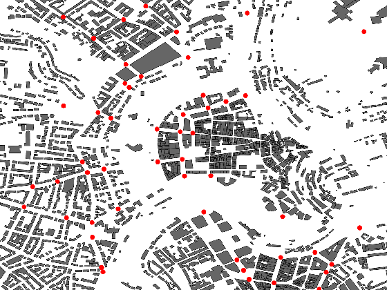
Figure 1: Real-world scenario: Luxembourg city center. The red circles represent the locations of the traffic lights, on top of which the gNBs in our scenario are placed.

III-A Mmwave vehicular network: Model and data trace

Our network system includes three main entities: gNBs $g\in\mathcal{G}$, beams $b\in\mathcal{B}$, and vehicles $v\in\mathcal{V}$. Also, time is divided in discrete intervals $k\in\mathcal{K}$. To add a dose of realism to our problem formulation, we consider the scenario representing the real-world topology of Luxembourg City, Luxembourg, and the realistic mobility therein, as reported by the publicly-available, large-scale trace described in [24]. Luxembourg city is chosen partly due to the availability of open-source trace data, but also because its urban layout represents a typical European city. The trace includes the location of traffic lights and bus stops, and the traffic lights states (red, yellow, green) at all time steps. It represents around 14,000 vehicles over a period of 12 hours, generated with SUMO, an open source multi-modal traffic simulator, and based on real-world traffic flows, e.g., commuters traveling to the city center. Depicted in Fig. 1 is the $2$ km $\times 2$ km area of the city center we take into consideration. Throughout this road topology, we place a total of 51 gNBs, colocated to traffic lights (their positions are marked by red dots in Fig. 1); the traffic lights corresponding to intersections with highest vehicle density were selected.

The gNBs and the vehicles are equipped with uniform planar array (UPA) antennas, composed of a grid of antenna elements spaced by $\lambda/2$. The vehicle UPA is only capable of analog beamforming (it is equipped with a single radio frequency (RF) chain). Digital beamforming is instead enabled at the gNBs, with $N(g)$ being the maximum number of beams that can be simultaneously active at the generic gNB $g$. We also denote by $P_{tot}(g)$ the total power budget the gNB has to split among its beams. As for the antenna elements, we consider two different models:

• the isotropic radiation antenna element denoted as “ISO”;

• the 3GPP sectored antenna element [11], denoted by “3GPP”, which is characterized by an 8 dBi maximum directional gain, significantly smaller side lobes than the ISO element, and higher front-to-back ratio. In this case, a three-sector gNB implementation is assumed, and the corresponding beamforming vector is used to shift the beam within each $120^{\circ}$ sector.

In this scenario, the goal is to make beamforming decisions that maximize the aggregated data rate over the vehicular users. We focus on downlink communications, although the analysis can easily be extended.

Such decisions concern:

• the number of active beams at each gNB,

• their width and direction, and

• the transmission power assigned to each beam.

The decisions are made at the gNBs every time step $k$, which coincides with the channel coherence time. For simplicity, we assume perfect channel state information (CSI) knowledge at the gNB. We consider that a beamshifting vector is used at the gNB to point the beam towards the desired direction, as described in Sec. III-B, while the width of the beam can be selected from a limited set of beamwidths, which can be obtained by varying the number of antenna elements employed.

The gNB transmits a single data stream towards one or more vehicles. As envisioned in 5G NR, data transmissions are organized into time slots, during which the channel is assumed to be constant. Thus, we can consider that, during data transfers, pilot symbols (the so-called DeModulation Reference Symbols (DMRS)) are transmitted in every time slot to adapt the modulation scheme to the instantaneous channel conditions. Below, we will denote by $C$ the number of slots per time step, and by $S$ the number of symbols per slot.

III-B Mmwave communication model

Given a gNB, $g$, and consider that the orientation in space of its antenna elements is characterized by the azimuth-elevation pair of angles $\boldsymbol{\psi}^{(g)}=[\psi^{(g)}_{1},\psi^{(g)}_{2}]$, as depicted in Fig. 2.

The orientation of the antenna elements at vehicle $v$ is represented by the pair of angles $\boldsymbol{\psi}^{(v)}=[\psi^{(v)}_{1},\psi^{(v)}_{2}]$, while the azimuth-elevation angle of the vehicle $v$, as observed by the gNB $g$ during time step $k$, is denoted by ${\bf d}=[d_{1},d_{2}]$.

At every time step $k$, the gNB adjusts the antenna gains to generate one or more beams. The number of beams to be generated is decided by the beam design algorithm. Let us focus on the generic beam $b$, with azimuth-elevation angle $\boldsymbol{\delta}^{(g)}$. To generate the beam, the gNB employs the beamforming vector ${\bf v}(\boldsymbol{\varphi}^{(g)})$ of size $N_{t}=N_{t,1}\times N_{t,2}$, with $n$-th element:

$$[{\bf v}(\boldsymbol{\varphi}^{(g)})]_{n}=\frac{1}{\sqrt{N_{t}}}{\rm e}^{{\rm j}\pi(n_{1}\cos\varphi^{(g)}_{2}\sin\varphi^{(g)}_{1}+n_{2}\sin\varphi^{(g)}_{2})}$$ (1)

where the integers $n_{1}\in\{1,\ldots,N_{t,1}\}$ and $n_{2}\in\{1,\ldots,N_{t,2}\}$ are such that $n=n_{1}N_{t,2}+n_{2}$. The vector of angles $\boldsymbol{\varphi}^{(g)}=\boldsymbol{\delta}^{(g)}-\boldsymbol{\psi}^{(g)}$ represents the direction of the beam with respect to the transmitting antenna orientation $\boldsymbol{\psi}^{(g)}$. If $\boldsymbol{\delta}^{(g)}={\bf d}$, then the beam of the transmitter is perfectly aligned with the vehicle on both the azimuth and elevation planes.

The symbols transmitted by the gNB in the $c$-th slot, $c=1,\ldots,C$, are represented by the vector ${\bf x}_{c}=[x_{c,1},\ldots,x_{c,S}]^{\mathsf{T}}$ whose elements are modeled as independent, complex random variables with zero-mean and variance $\mathbb{E}[|x_{c,s}|^{2}]=P$ ($s=1,\ldots,S$) where $P$ is the power of the considered beam. In the following, for simplicity, we omit the argument $\boldsymbol{\varphi}^{(g)}$ of the beamforming vector ${\bf v}$.

Figure 2: mmwave communication beams and notations used.

The signal transmitted by the gNB in the $c$-th slot is represented by the $N_{t}\times S$ matrix ${\bf v}{\bf x}_{c}^{\mathsf{T}}$ and the corresponding signal received by the vehicle is described by the $N_{r}\times S$ matrix ${\bf Y}$, with $N_{r}=N_{r,1}\times N_{r,2}$:

$${\bf Y}_{c}={\bf H}_{c}{\bf v}{\bf x}_{c}^{\mathsf{T}}+{\bf E}_{c}\,.$$ (2)

In (2), ${\bf H}_{c}$ is the $N_{r}\times N_{t}$ channel matrix between gNB $g$ and vehicle $v$ during the transmission on the $c$-th slot, while ${\bf E}_{c}$ is a term accounting for noise and interference. Note that nearby gNBs cause interference if the radiation pattern of their beams affects the vehicle reception.

In a typical mmwave urban scenario, the channel between the transmitter and the receiver is composed of a number of path clusters, each cluster corresponding to a macro-level scattering path. The $\ell$-th path is described by its amplitude, $h_{\ell,c}$, and the azimuth-elevation departure and arrival pairs of angles $\boldsymbol{\vartheta}^{(g)}_{\ell,c}$ and $\boldsymbol{\vartheta}^{(v)}_{\ell,c}$, measured with respect to the antenna orientation angles $\boldsymbol{\psi}^{(g)}$ and $\boldsymbol{\psi}^{(v)}$, respectively. Using the model provided in [10, 9, 11], the channel matrix during the $c$-th slot, ${\bf H}_{c}$, can be modeled as

$${\bf H}_{c}=\sqrt{\frac{1}{L}}\sum_{\ell=1}^{L}h_{\ell,c}{\bf a}_{v}(\boldsymbol{\vartheta}^{(v)}_{\ell,c}){\bf a}_{g}(\boldsymbol{\vartheta}^{(g)}_{\ell,c})^{\mathsf{H}}$$ (3)

where $L$ is the number of paths, and ${\bf a}_{g}(\boldsymbol{\vartheta})$ and ${\bf a}_{v}(\boldsymbol{\vartheta})$ are the response vector for, respectively, the transmit and the receive antenna. More specifically, the $n$-th element of ${\bf a}_{g}(\boldsymbol{\vartheta})$ is:

$$[{\bf a}_{g}(\boldsymbol{\vartheta})]_{n}={\rm e}^{{\rm j}\pi(n_{1}\cos\vartheta_{2}\sin\vartheta_{1}+n_{2}\sin\vartheta_{2})}$$ (4)

where $n_{1}\in\{1,\ldots,N_{t,1}\}$ and $n_{2}\in\{1,\ldots,N_{t,2}\}$ are such that $n=n_{1}N_{t,2}+n_{2}$. Similarly, the $n$-th element of ${\bf a}_{v}(\boldsymbol{\vartheta})$ is given by

$$[{\bf a}_{v}(\boldsymbol{\vartheta})]_{n}={\rm e}^{{\rm j}\pi(n_{1}\cos\vartheta_{2}\sin\vartheta_{1}+n_{2}\sin\vartheta_{2})}$$ (5)

where $n_{1}\in\{1,\ldots,N_{r,1}\}$ and $n_{2}\in\{1,\ldots,N_{r,2}\}$ are such that $n=n_{1}N_{r,2}+n_{2}$. The $N_{r}\times S$ matrix ${\bf E}_{c}$ in (2) has complex Gaussian independent entries, and its columns ${\bf e}_{c,s}$ have zero mean and covariance $\mathbb{E}[{\bf e}_{c,s}{\bf e}_{c,s}^{\mathsf{H}}]=I_{c}{\bf I}$ ($s=1,\ldots,S$). Since the vehicle UPA is only capable of analog beamforming, we consider that the weight vector ${\bf w}(\boldsymbol{\varphi}^{(v)})$ of size $N_{r}$ is applied to the RF chain, with generic element:

$$[{\bf w}(\boldsymbol{\varphi}^{(v)})]_{n}={\rm e}^{{\rm j}\pi(n_{1}\cos\varphi^{(v)}_{2}\sin\varphi^{(v)}_{1}+n_{2}\sin\varphi^{(v)}_{2})}\,,$$ (6)

in order to generate a beam with azimuth-elevation angle $\boldsymbol{\delta}^{(v)}=\boldsymbol{\varphi}^{(v)}+\boldsymbol{\psi}^{(v)}$. The integers $n_{1}\in\{1,\ldots,N_{r,1}\}$ and $n_{2}\in\{1,\ldots,N_{r,2}\}$ are such that $n=n_{1}N_{r,2}+n_{2}$. This scenario is illustrated in Fig. 2. If $\delta^{(v)}_{1}={\rm mod}(180^{\circ}+d_{1},360)$ and $\delta^{(v)}_{2}=180-d_{2}$, then the receiver’s beam is perfectly aligned with the gNB, in azimuth and elevation.

Through the weighting procedure, the receiver forms the vector

${\bf z}_{c}={\bf w}^{\mathsf{H}}{\bf Y}_{c}=\widetilde{h}_{c}{\bf x}_{c}^{\mathsf{T}}+{\bf w}^{\mathsf{H}}{\bf E}_{c}$

where

$$\widetilde{h}_{c}={\bf w}^{\mathsf{H}}{\bf H}_{c}{\bf v}$$ (7)

is the scalar channel coefficient summarizing the effects of the signal propagation conditions and of the antenna and beam design. For simplicity, in the above equations, we omitted the argument $\boldsymbol{\varphi}^{(v)}$ of ${\bf w}$. Finally, estimates of the symbols belonging to the $c$-th slot are obtained at the receiver by processing the vector ${\bf z}_{c}$.

Note that, if more than one gNB transmits toward the same user in such a way that it causes constructive interference (CoMP-like mode), similar expressions to the ones above hold, where ${\bf H}_{c}{\bf v}$ represents the equivalent channel.

IV A Convenient Statistical Model of the Channel Gain

In this section, we provide a statistical characterization of the channel gain under different antenna models and beam alignment conditions, and we show its validity in the real-world scenario represented by the Luxembourg trace, depicted in Fig. 1. Note, however, that our model has general validity and can be used for the study of aspects beyond the scope of this work.

We start by applying two channel models, among those which appeared in the literature, that are most commonly used:

• the “NYU” model [9], a statistical spatial channel model based on experimental measurements performed in the city of New York;

• the “3GPP” model [11], a hybrid of geometry-based stochastic and map-based channel models, which has been adopted by 3GPP.

Both these models describe the channel between two communicating endpoints as composed of several clusters of paths, each synthesized using a large number of subpaths, with certain azimuth and elevation arrival and departure angle.

In the following, we implement both the above models and, using link-level simulations, we provide a statistical characterization of the channel gain $\widetilde{h}_{c}$ as defined in (7).

Figure 3: The case of full alignment along the Azimuth ((a), (b), and (c)) cases), and the case of misaligned beams (d).

Given the channel matrix ${\bf H}_{c}$ given in (3), the beam directions (specified by the weight vectors ${\bf v}$ and ${\bf w}$), and the relative positions between transmitter and receiver, we characterize the gain of the channel connecting gNB $g$ to vehicle $v$ during the transmission in the $c$-th slot. To this end, we rewrite (7) as:

$$|\widetilde{h}_{c}|^{2}=aG$$ (8)

where $a$ is the path loss between the gNB-vehicle pair as a function of their distance, and the gain component, $G$, encompasses both the small-scale fading effects of the channel and the beamforming gain of the antenna array.

The value of $G$ has a strong dependence on the degree of alignment between the beams; under line of sight (LoS) conditions, we have three cases:

• “fully a-aligned” link, where both beams are perfectly aligned with each other along the azimuth,

• “partially a-aligned” link where the beams are aligned along the azimuth at only one end, at either the transmitter or the receiver side, and

• “misaligned” link where neither beam is aligned.

The accurate description of the behaviour of gain $G$ in these three cases is critical in modeling the useful power and interference levels at the receiver side, especially in the presence of LoS. In particular, we differentiate between the partially a-aligned and fully misaligned cases, since simulations show that the gain can be significantly higher when the beam is aligned at one end, as opposed to when it is misaligned at both ends. The partially a-aligned gain can be applied to model more accurately the interference experienced at the receiver, especially in those cases where a vehicle may be inadvertently under the coverage of an interfering gNB, or to describe the constructive interference in the context of CoMP-like cases.

In the following subsections, we empirically characterize the distribution of the gain $G$ under the above described propagation conditions and for the two different antenna radiation patterns. For each scenario, we show that the empirical distribution of $G$, can be tightly approximated by using Gaussian, exponential, or log-logistic distributions.

IV-A Fully a-aligned beams and 3GPP channel

When LoS conditions hold and the beams of the transmitter and of the receiver are perfectly aligned in the azimuth plane (a-aligned), we found that, under the “3GPP” channel model, the distribution of the gain $G$ is well approximated by a Gaussian distribution with mean $\mu_{G}$ and variance $\sigma_{G}^{2}$.

Specifically, when ISO antenna elements are employed, the mean $\mu_{G}$ is given by

$$\mu_{G}(\Delta_{2})=\mu_{0}\exp\left(-\frac{\Delta_{2}^{2}}{\gamma_{\mu}^{2}}\right)\,.$$ (9)

Since we do not consider perfect alignment on the elevation plane, our analysis shows that the parameter $\mu_{G}$ depends on the angle of misalignement in the elevation plane, denoted by $\Delta_{2}$ (see Fig. 3-(c) for details). When instead 3GPP antenna elements are used, $G$ also depends on the angle $\Delta_{1}$ between the direction of the beam at the gNB and the direction of the sector center (see Fig. 3-(b)). In particular, the resulting gain is reduced when the beam at the gNB is not aligned with the direction of the sector, and it becomes 0 for a beam out of the sector width, as per the 3GPP antenna element radiation pattern [11]. The mean $\mu_{G}$, for the 3GPP antenna element, is given by:

$$\mu_{G}(\Delta_{1},\Delta_{2})=\mu_{0}\exp\left(-\frac{\Delta_{2}^{2}}{\gamma_{\mu}^{2}}\right)10^{-1.2\left(\frac{\Delta_{1}}{\theta_{\rm 3dB}}\right)^{2}}$$ (10)

where $\theta_{\rm 3dB}=65^{\circ}$ is the half-power beamwidth of a single antenna element. With regard to the standard deviation $\sigma_{G}$, in both the ISO and 3GPP cases, it depends on $\Delta_{2}$ according to the relation:

$$\sigma_{G}(\Delta_{2})=\sigma_{0}\exp\left(-\frac{\Delta_{2}^{2}}{\gamma_{\sigma}^{2}}\right)\,.$$ (11)

Finally, we established a dependence between the parameters $\mu_{o},\sigma_{0},\gamma_{\mu},\gamma_{g}$ and the product $N_{t}N_{r}$, captured by the expressions provided in Table II.

TABLE II: Values of the parameters characterizing the distribution of $G$, for fully a-aligned beams and 3GPP channel model

	ISO	3GPP
$\mu_{0}$	$0.537(N_{t}N_{r})^{0.998}$	$3.26(N_{t}N_{r})$
$\sigma_{0}$	$0.23(N_{t}N_{r})^{0.7}$	$1.33(N_{t}N_{r})^{0.65}$
$\gamma_{\mu}$	$55.02(N_{t}N_{r})^{-0.287}$	$49.01(N_{t}N_{r})^{-0.274}$
$\gamma_{\sigma}$	$55.86(N_{t}N_{r})^{-0.28}$	$55.86(N_{t}N_{r})^{-0.28}$

Fig. 4 compares the empirical distribution of the gain $G$ to the Gaussian distribution whose parameters are specified in (9)–(11). The plots of the probability density function (PDF) of the gain have been obtained under the 3GPP channel model, for both ISO and 3GPP antenna model. Importantly, our proposed approximation is very tight in both cases; furthermore, it holds also for other values of the number of antennas, $\Delta_{2}$, and $\Delta_{1}$ (for the 3GPP antenna model).

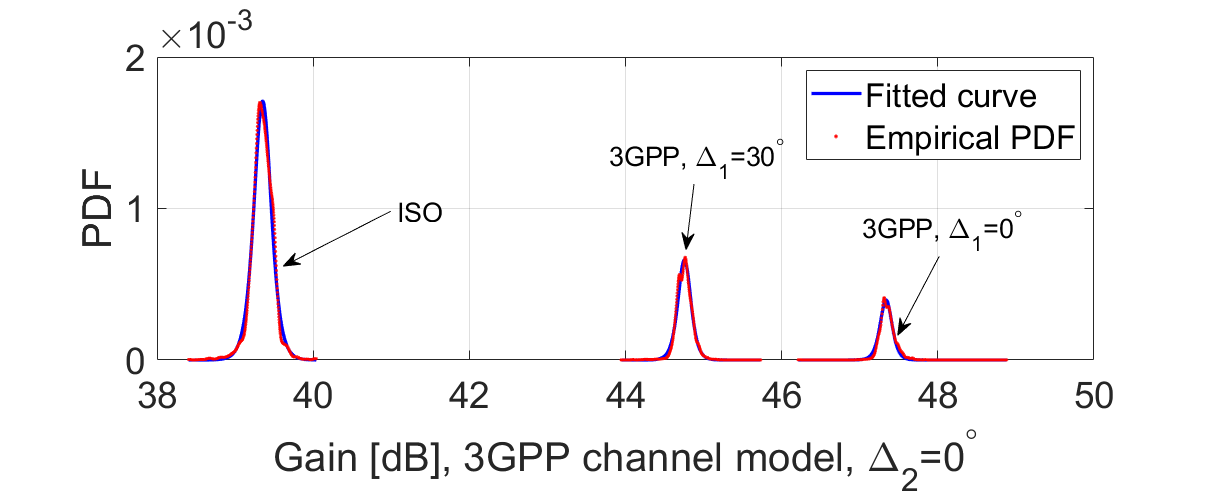
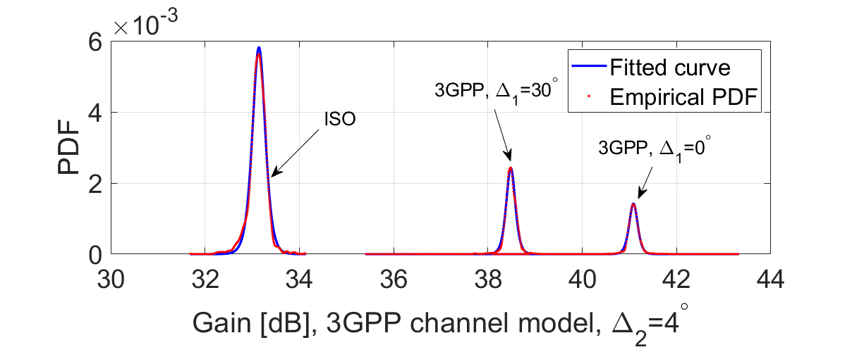
Figure 4: LoS and fully a-aligned case: Empirical and fitted distribution of $G$ under the 3GPP channel model, and when the ISO and 3GPP antennas are employed. $\Delta_{2}=0^{\circ}$ (top) and $\Delta_{2}=4^{\circ}$ (bottom). $N_{t}=256$, $N_{r}=64$.

To be able to compare to the no line of sight (NLoS) case, we derived the results shown in Fig. 5 (left). In NLoS conditions, the values of $G$ drop significantly and the gain distribution can be better approximated with the log-logistic distribution:

$$f_{G}(x)=\frac{1}{mx}\frac{e^{z}}{(1+e^{z})^{2}}$$ (12)

where $z=(\log(x)-m)/s$.

Due to the absence of the LoS path, no significant dependency on the misalignment elevation angle $\Delta_{2}$ could be inferred, nor a straightforward relationship to the product $N_{t}N_{r}$. However, as shown in Table III, the values of the distribution parameters $m$ and $s$ vary depending on the channel model/antenna type considered, and the number of antennas $N_{t}$ and $N_{r}$. Due to space limitations, in Fig. 5, we only show the results for the ISO antenna elements, however the approximations hold as well when 3GPP antenna elements are used.

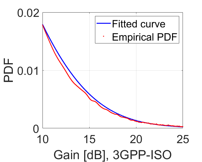
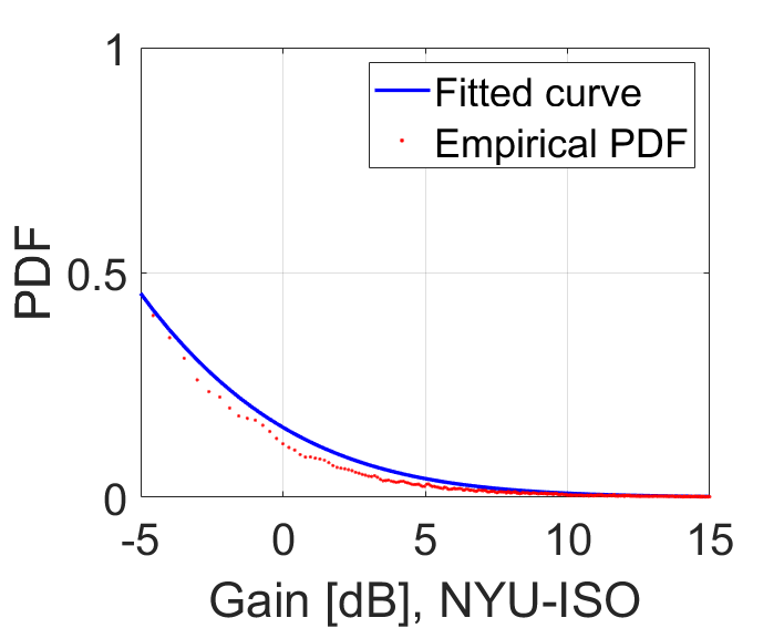
Figure 5: NLoS conditions: Empirical and fitted distribution of gain $G$ under the 3GPP channel model (left) and the NYU channel model (right), when ISO antennas are employed. $N_{t}=256$, $N_{r}=64$.

TABLE III: Values of the parameters characterizing the distribution of $G$, when the beams are a-aligned in NLoS

(m,s)	$N_{t}=256$	$N_{t}=64$	$N_{t}=64$
	$N_{r}=64$	$N_{r}=64$	$N_{r}=16$
3GPP-ISO	$(2.97,0.99)$	$(3.83,0.98)$	$(3.28,0.97)$
3GPP-3GPP	$(4.63,1)$	$(5.57,0.99)$	$(4.98,0.98)$
NYU ISO	$(-1.7,0.97)$	$(-1.98,0.97)$	$(-2.75,0.95)$
NYU 3GPP	$(-2.6,1.03)$	$(-3.68,2.72)$	$(-0.48,1.1)$

IV-B Fully a-aligned beams and NYU channel

Now, we still consider fully a-aligned beams, but we focus on the NYU channel model. In this case and under LoS conditions, we find that the empirical distribution of the gain $G$ is tightly approximated by an exponential distribution with average $\alpha_{G}$, i.e., $f_{G}(x)=\frac{1}{\alpha_{G}}\exp\left(-\frac{x}{\alpha_{G}}\right)$. In particular, when ISO antenna elements are employed, the parameter $\alpha_{G}$ depends on $\Delta_{2}$ according to $\alpha_{G}(\Delta_{2})=\alpha_{0}\exp\left(-\frac{\Delta_{2}^{2}}{\gamma_{\alpha}^{2}}\right)$. Instead, with 3GPP antenna elements, $\alpha_{G}$ depends on both $\Delta_{1}$ and $\Delta_{2}$, according to the relation:

$$\alpha_{G}(\Delta_{1},\Delta_{2})=\alpha_{0}\exp\left(-\frac{\Delta_{2}^{2}}{\gamma_{\alpha}^{2}}\right)10^{-1.2\left(\frac{\Delta_{1}}{\theta_{3dB}}\right)^{2}}$$ (13)

where $\theta_{\rm 3dB}=65^{\circ}$. Interestingly, the values of the parameters $\alpha_{0}$ and $\gamma_{\alpha}$ can be expressed as functions of the product $N_{t}N_{r}$, as shown in Table IV.

TABLE IV: Values of the parameters of the distribution of $G$, under LoS and NYU channel model

	ISO	3GPP
$\alpha_{0}$	$0.63(N_{t}N_{r})^{1.05}$	$5.2(N_{t}N_{r})^{1.03}$
$\gamma_{\alpha}$	$54.85(N_{t}N_{r})^{-0.3}$	$54.85(N_{t}N_{r})^{-0.3}$

Examples of the empirical and fitted distribution of $G$ are provided in Fig. 6 when the gNB is equipped with ISO and 3GPP antenna elements, and for different values of $\Delta_{1}$ and $\Delta_{2}$.

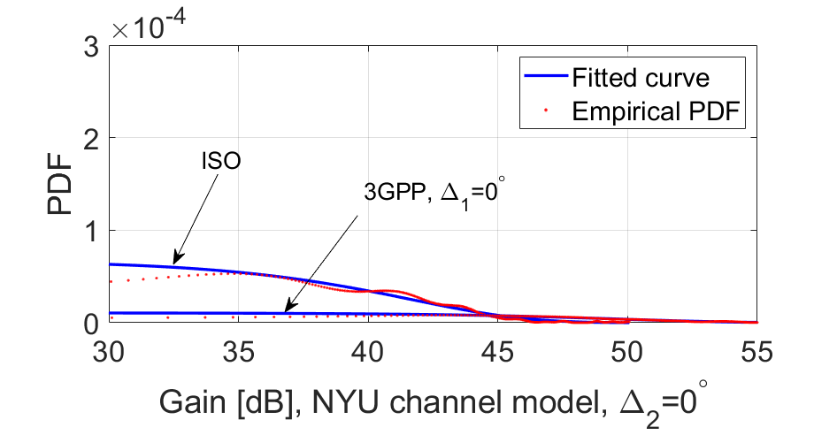
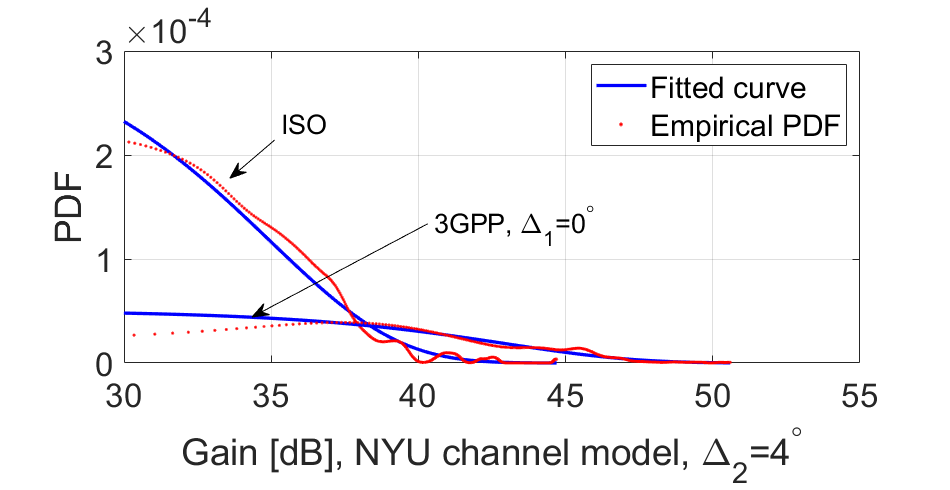
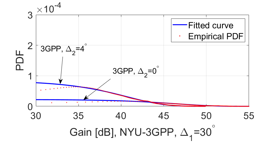
Figure 6: LoS and fully a-aligned case: Empirical and fitted distribution of $G$ under the NYU channel model and when ISO and 3GPP antennas are employed. $\Delta_{2}=0^{\circ}$ (left), $\Delta_{2}=4^{\circ}$ (middle), and $\Delta_{1}=30^{\circ}$ (right) . $N_{t}=256$, $N_{r}=64$, and $\Delta_{1}=0^{\circ}$ for 3GPP antennas.

Again, there is a very close match between the experimental distribution of the gain and our analytical approximation, which holds also for different values of numbers of antennas, $\Delta_{2}$, and $\Delta_{1}$.

Similarly to the 3GPP channel model, in the absence of LoS, the a-aligned gain for the NYU channel model is better approximated using the log-logistic distribution, given by (12), however different values for parameters $m$ and $s$ are applied, as reported in Table III. The empirical distribution and the fitted counterpart are shown in the right plot in Fig. 5.

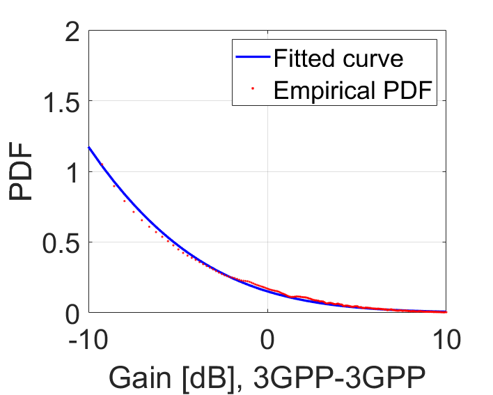
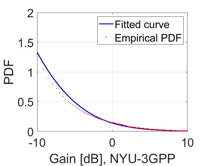
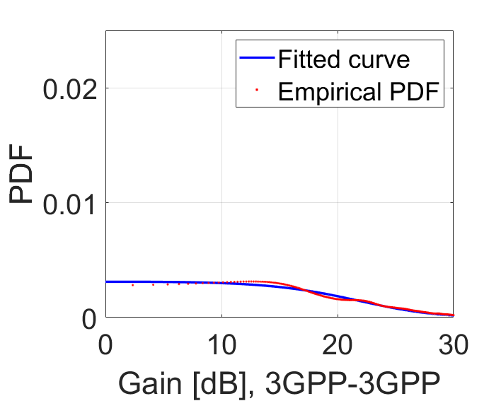
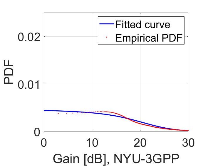
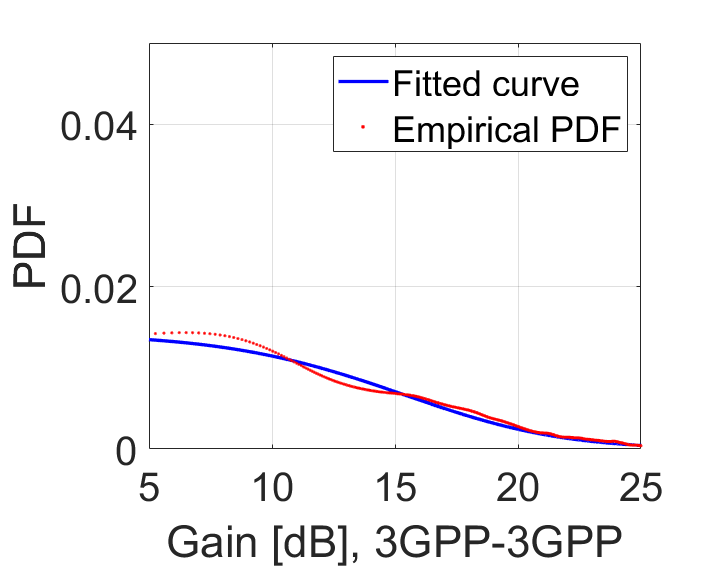
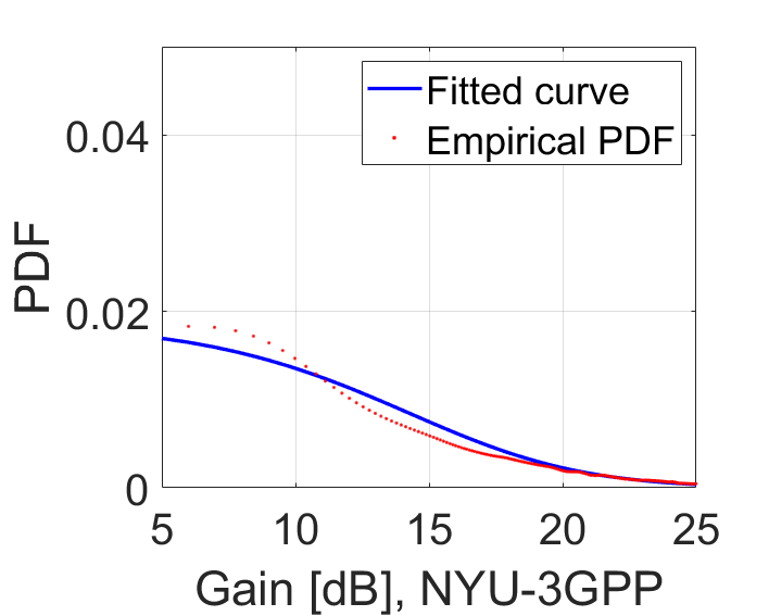
Figure 7: Empirical and fitted distribution of gain $G$, for the 3GPP (left) and the NYU (right) channel model when 3GPP antennas are employed, in the case of full misalignment (top), partial a-alignment at the transmitter (middle) and partial a-alignment at the receiver (bottom). $N_{t}=256$, $N_{r}=64$.

IV-C Partially a-aligned or misaligned beams

When the beams are partially a-aligned or misaligned, we found that the empirical distribution of $G$ can be approximated with the log-logistic distribution reported in (12)

The approximation is valid for all considered channel models and antenna elements, however the values of the parameters $m$ and $s$ vary depending on the type of misalignment. Namely, we consider three cases of misalignment: 1) full misalignment where beams both at the transmitter and receiver are not aligned, 2) the partial a-alignment at the transmitter side, where the beam at the transmitter is aligned but not at the receiver, and 3) the partial a-alignment at the receivers side, where the beam at the receiver is aligned but not at the transmitter.

TABLE V: Values of the parameters characterizing the distribution of $G$, when the beams are partially a-aligned or misaligned

$(m,s)$	$N_{t}=256$	$N_{t}=64$	$N_{t}=64$
	$N_{r}=64$	$N_{r}=64$	$N_{r}=16$
3GPP-ISO	1. $(-2.5,1)$	$1.(-1.45,1)$	$1.(-1.65,1)$
	2.$(3.89,0.99)$	$2.(3.2,0.99)$	$2.(3.15,0.85)$
	3.$(2.35,0.98)$	$3.(3.2,0.99)$	$3.(1.9,0.98)$
3GPP-3GPP	1.$(-1.05,1)$	1.$(-0.16,1)$	1.$(0.01,1)$
	2.$(5.72,0.99)$	2.$(5.05,0.99)$	2.$(4.99,0.86)$
	3.$(4.16,0.98)$	3.$(5.03,0.99)$	3.$(3.79,0.98)$
NYU ISO	1.$(-1.96,1.01)$	1.$(0.59,1.01)$	1.$(-0.17,1.06)$
	2.$(3.77,0.99)$	2.$(3.3,1)$	2.$(2.97,0.98)$
	3.$(2.17,0.98)$	3.$(2.94,0.99)$	3.$(1.8,0.98)$
NYU 3GPP	$1.(-1.48,0.97)$	$1.(1.65,0.99)$	$1.(-0.97,1.05)$
	2.$(5.48,0.99)$	2.$(4.99,1)$	2.$(4.76,0.98)$
	3.$(3.95,0.99)$	3.$(4.75,0.99)$	3.$(3.51,0.98)$

Unlike in the fully a-aligned case, in the partially a-aligned case, no evident dependency could be established between the misalignment angle in the azimuth plane and the values of the distribution parameters $m$ and $s$. This is due to the fact that the misalignment angle only determines the contribution to the gain coming from the side-lobes of the misaligned end, while the dominant contribution to the resulting effective gain comes from the main lobe of the aligned end, which is not affected by this angle. Hence, the dependency of the gain on the misalignment angle tends to vanish and no characterization of it is possible. Similarly, although it is evident that the parameters of the distribution $m$ and $s$ are affected by the number of antennas $N_{t}$ and $N_{r}$, no straightforward relationship can be established. The numerically evaluated values for the parameters $m$ and $s$ are provided in Table V, for all possible combinations of channel model and antenna elements (across rows) and for several values of $N_{t}$ and $N_{r}$ (across columns). In each cell of the table, the three lines correspond, respectively, to misalignment at both transmitter and receiver, alignment at the transmitter only, and alignment at the receiver only.

A close match can be observed between the empirical samples and the fitted distributions, in Fig. 7 for misaligned links (top), partially a-aligned links at the transmitter (middle) and partially a-aligned links at the receiver (bottom). The plots shown were obtained for both channel models and the 3GPP antenna element, with $N_{t}=256$, $N_{r}=64$. Similar plots were obtained for the ISO antenna elements, but were omitted for brevity. Random values of misalignment angles $\Delta_{1}$ and $\Delta_{2}$ were generated to obtain the empirical probability distribution functions. Furthermore, by looking at the support of the distribution in Figs. 4– 7, it can be observed how significant the impact of partial alignment can be: the probability distribution is indeed spread over significantly higher values of $G$ for the partially a-aligned link with respect to the misaligned case, although about 20 dB smaller than the fully a-aligned case.

IV-D System-level validation of the channel approximations

We now validate the above approximations at the system level. To do so, we consider the realistic mmwave vehicular network described in Sec. III-A. However, due to the complexity of fully simulating the 3GPP and the NYU channel models, we only consider a $0.4km\times 0.4km$ area in the center of Luxembourg city, i.e., 8 gNBs and around 120-140 vehicles served at each 1 s-time step.

Each gNB, equipped with $N_{t}=256$ antennas, enables a single beam with a static direction chosen at random. Each vehicle is instead equipped with $N_{r}=64$ antennas and is associated to the closest gNB. To quantify the network perfomance, we calculate the signal-to-interference-and-noise ratio (SINR) for each vehicle $v$ as:

$${\rm SINR}_{v}=\frac{P(g^{\star})|\tilde{h}_{c}(g^{\star},v)|^{2}}{N_{0}+\sum_{g\in\mathcal{G}\land g\neq g^{\star}}P(g)|\tilde{h}_{c}(g,v)|^{2}}$$ (14)

where $g^{\star}$ is the gNB to which the vehicle is associated, and $N_{0}$ is the white noise power. The achievable data rate is then:

$$R(b,k,v)=B_{w}\log\left(1+{\rm SINR}_{v}\right)$$ (15)

where $B_{w}$ is the channel bandwidth. The values of data rate we obtained through Monte Carlo simulations of the channel coefficients are compared to the values obtained using the approximated channel gains. More specifically, the approximate gains $G(b,v)$ in (8) are generated for each gNB-beam-vehicle triple, by drawing random values from the distributions obtained in the previous subsections, depending on the level of alignment between their respective beams and LoS conditions. Fig. 8 shows the cumulative distribution function (CDF) curves of the data rate values obtained under the 3GPP (top) and the NYU (bottom) channel model, both for the sectored 3GPP and ISO antenna elements. In both cases, the curves derived under full 3GPP channel simulation fit well with our proposed approximations, which leverage the distributions derived in Secs. IV-A and IV-C. Similar results were obtained for the SINR, but were omitted for brevity. These plots show that the data rate achieved under the approximated channel models, closely matches that recorded under the actual 3GPP and NYU models, with negligible deviations for the low-SINR vehicles. Importantly, these results allow us to substantially simplify the mmwave channel model, while maintaining an adequate level of realism in our scenario.

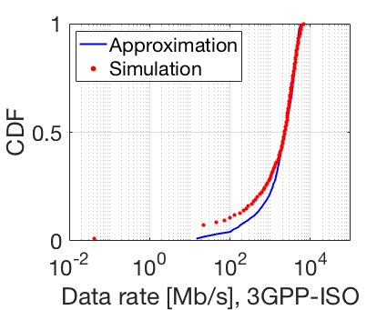
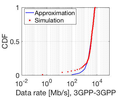
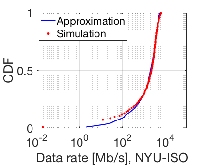
Figure 8: CDF of the achievable rate obtained via system-level simulations of the Luxembourg scenario, for the 3GPP (top) and the NYU (bottom) channel model, and for ISO (left) and 3GPP (right) antennas. The approximation values were obtained applying the models in Secs. IV-A and IV-C.

V gNB Selection and Beam Design

We now leverage the channel gain model described above and focus on the main aspects of traffic delivery in mmwave vehicular networks and on the approach we propose to overcome the existing hurdles. In particular, Sec. V-A introduces the beam design problem and our optimization formulation, formally stating its objective and constraints. Then Sec. V-B presents the heuristic approaches we investigate, among which our proposed scheme, TL.

V-A Optimization formulation

Given the system model presented above, here we aim to answer the following questions: i) how many beams should be active at each gNB, and of what beamwidth; ii) which directions should they point at on the azimuth plane; and, finally, iii) which user should be scheduled on which beam. The goal is to find answers to these questions that maximize the total users’ data rate.

In the following section, we present an optimization formulation of the beam management problem, to be solved at every time step $k$.

For each gNB $g$, we are given the maximum number $N(g)$ of beams that can be created, their maximum half-power width $A(g)$ (which is equal to the sector amplitude in the case of 3GPP antennas), as well as the total power budget $P_{tot}(g)$ that has to be split across the gNB beams. We also know the angles, ${\bf d}(g,k,v)$, representing the azimuth and the elevation of vehicle $v$ as seen from the gNB $g$ at time $k$ (see Sec. III-B and Fig. 2).

To make our decisions, we have to set many variables. Binary variable $\gamma(b,g,k)$ expresses whether beam $b$ is used (i.e., emitted) by gNB $g$ at time $k$; such a dynamic relationship between gNBs and beams allows us to represent the fact that the same gNB may have a different number of beams at different times. Continuous variables $\alpha(b,k)$, $\delta_{1}^{(g)}(b,k)$, and $P(b,k)$, respectively express the half-power width, directions, and power of beam $b$ at time $k$. Furthermore, for each pair of beams $(b_{1},b_{2})$ with $b_{2}\neq b_{1}$, we can use $b_{1}$ to generate constructive interference (CoMP-like) with $b_{2}$, or to avoid destructive interference by keeping it silent (ABS-like), which is modeled through binary variables $\mu(b_{1},b_{2},k)$ and $\beta(b_{1},b_{2},k)$, respectively. E.g., $\mu(b_{1},b_{2},k)=1$ means that, at time $k$, beam $b_{1}$ is used to improve the data rate of $b_{2}$ instead of transmitting data on its own. Finally, continuous variables $\sigma(b,k,v)\in[0,1]$ express the fraction of time that beam $b$ allocates to serve vehicle $v$ at time $k$.

To begin with, we impose that each beam only belongs to one gNB at every time interval, and that gNBs do not exceed the maximum number of beams. I.e., for any $k\in\mathcal{K}$,

$$\sum_{g\in\mathcal{G}}\gamma(b,g,k)\leq 1,\,\,\,\forall b\in\mathcal{B};\quad\sum_{b\in\mathcal{B}}\gamma(b,g,k)\leq N(g),\,\,\,\forall g\in\mathcal{B}\,.$$ (16)

In particular, the first inequality descends from the fact that, in our model, beams in $\mathcal{B}$ are not statically tied to a specific gNB; thus, the same element of $\mathcal{B}$ cannot be associated with multiple gNBs at the same time.

Furthermore, we must ensure that the half-power width of the beams does not exceed the limit, and that beams of the same gNB do not overlap:

$$\alpha(b,k)\leq A(U(b,k)),\quad\forall b\in\mathcal{B},k\in\mathcal{K},$$ (17)

$$|\delta_{1}^{(g)}(b_{1},k)-\delta_{1}^{(g)}(b_{2},k)|\geq\frac{\alpha(b_{1},k)+\alpha(b_{2},k)}{2},\\ \forall b_{1},b_{2}\in\mathcal{B}\colon U(b_{1},k)=U(b_{2},k),k\in\mathcal{K}.$$ (18)

In both (17) and (18), $U(b,k)=g\in\mathcal{G}\colon\gamma(b,k,g)=1$ represents the gNB to which beam $b$ belongs.

TABLE VI: Notation used in the formulation of the optimization problem

Symbol	Type	Meaning
$A(g)$	parameter	Max half-power width of beams of gNB $g$
$\alpha(b,k)$	continuous var.	Half-power width of beam $b$ at $k$
$\sigma(b,k,v)$	continuous var.	Fraction of time step $k$ that beam $b$ uses to serve vehicle $v$
$\mu(b_{1},b_{2},k)$	binary var.	Whether beam $b_{1}$ supports in a COMP-like fashion beam $b_{2}$ at $k$
$\beta(b_{1},b_{2},k)$	binary var.	Whether beam $b_{1}$ supports in an ABS-like fashion beam $b_{2}$ at $k$
$\gamma(b,g,k)$	binary var.	Whether beam $b$ is used by gNB $g$ at $k$
$U(b,k)$	auxiliary var.	gNB using beam $b$ at $k$
$V(b,k,v)$	auxiliary var.	Whether beam $b$ covers vehicle $v$ at $k$
$R(b,k,v)$	output	Data rate between beam $b$ and vehicle $v$ at $k$
$P(b,k)$	continuous var.	Power of beam $b$ at $k$

Concerning transmission power, we mandate that the per-gNB power budgets are met, and that no power is allocated to unused beams, i.e.,

$$\sum_{b\in\mathcal{G}\colon U(b,k)=g}P(b,k)\leq P_{tot}(g),\quad\forall g\in\mathcal{G},k\in\mathcal{K},$$ (19)

$$P(b,k)\leq\sum_{g\in\mathcal{G}}\gamma(b,g,k)P_{tot}(g),\quad\forall b\in\mathcal{B},k\in\mathcal{K}.$$ (20)

Finally, any beam $b$ can be used at any time $k$ in a COMP- or ABS-like fashion in combination with at another beam:

$$\sum_{b^{\prime}\in\mathcal{B}}\left[\mu(b,b^{\prime},k)+\beta(b,b^{\prime},k)+\mu(b^{\prime},b,k)+\beta(b^{\prime},b,k)\right]\leq 1\,.$$ (21)

Concerning the scheduling variables, we proceed as follows. The sum of variables $\sigma(b,k,v)$ cannot exceed one:

$$\sum_{v\in\mathcal{V}}\sigma(b,k,v)\leq 1,\quad\forall b\in\mathcal{B},k\in\mathcal{K}.$$ (22)

Additionally, we schedule no time to serve vehicles that are out of the beam’s coverage:

$$\sigma(b,k,v)\leq V(b,k,v),\quad\forall b\in\mathcal{B},k\in\mathcal{K},v\in\mathcal{V}.$$ (23)

In (23), $V(b,k,v)=\mathds{1}_{\{|\delta_{1}^{(g)}(b,k)-d(g,k,v)|\leq\alpha(b,k)/2\}}$ (with $g=U(b,k)$) represents whether beam $b$ covers vehicle $v$ at time $k$.

Our objective can then be stated as maximizing the total data rate received by vehicles:

$$\max_{\alpha,\beta,\gamma,\delta_{1}^{(g)},\mu,\pi,\sigma}\sum_{b\in\mathcal{B}}\sum_{k\in\mathcal{K}}\sum_{v\in\mathcal{V}}\sigma(b,k,v)R(b,k,v)$$ (24)

where $R(b,k,v)$ represents the data rate that vehicle $v$ would obtain from beam $b$ at time $k$, if that beam would serve no other vehicle. Given the availability of the channel coefficients at the gNB, during time step $k$, i.e., ${\bf H}_{k}$, and of the ${\rm SINR}_{v}$ in (14) experienced by the receiver, the gNB can transmit at the maximum data rate supported by the channel. Then, considering the very high waveform spectral occupancy in 5G, the achievable data rate through beam $b$ at time step $k$ is given by (15). In the case of a CoMP-like transmission, the useful signal (interference) is determined by the number of gNB contributing constructively (destructively), which are captured by the $V(b,k,v)$ variables. Note that, in this case, the total useful signal is given by the sum of signals coming from different gNBs, which coordinate among themselves and apply a precoding matrix in order to perform in-phase transmissions. It is also important to underline that $R(b,k,v)$ is the estimated achievable rate, while the actual data rate is determined by the instantaneous channel conditions and the modulation-coding scheme that is selected.

V-B Beam design heuristics

Directly solving the optimization problem stated in Sec. V-A has a very high computational complexity. Indeed, in both the unicast and brodcast cases, $R$ in the objective is a non-linear function of the decision variables, and some of the constraints, e.g., (18) and (23), involve an indicator function and/or the modulo operator, thus making the problem fall in the mixed-integer linear programming (MILP) category. Such problems are well-known to be NP-hard (the reader is referred to the reduction from the vertex cover problem in [25]).

To avoid dealing with such an overwhelming complexity, we adopt a heuristic approach.

Clustering-based strategies. We first cast the beam management problem as a one-dimensional clustering Indeed, each beam $b$ of gNB $g$ can be seen as a cluster of directions, with center $\delta_{1}^{(g)}(b,k)$ and maximum width $A(g)$. Each of such directions may cover one or more users at a given data rate, depending on the channel conditions and the antenna gain. Thus, each direction can be associated with a certain “weight” reflecting the sum rate offered to the covered users. Clustering will lead to maximizing the total weight corresponding to a set of directions (beams). We then solve the clustering problem by considering two different strategies, named Static and Dynamic, as detailed next.

In the Static scheme, the directions and widths of the beams at the gNBs do not change over time, i.e., $\delta_{1}^{(g)}(b,k)=\delta_{1}^{(g)}(b)$ and $\alpha(b,k)=\alpha(b)$. To determine those directions, we formulate a hierarchical clustering problem as follows:

1. for each vehicle $v$ and time step $k$, we create one observation (i.e., one data point) corresponding to $v$’s position;

2. we consider the whole set of observations and compute the pairwise angular distances (i.e., $|\delta_{1}^{(g)}(b,k)-d(g,k,v)|$ between any two observations;

3. we feed the resulting distance matrix to the Voor Hees algorithm [26], setting the maximum intra-cluster distance to $A(g)$;

4. we consider the $n$ largest clusters, i.e., the clusters including the highest number of observations;

5. for each such cluster, we set the direction $\delta_{1}^{(g)}(b)$ as the mean between the minimum and maximum angle of the vehicles it includes, i.e., $\delta_{1}^{(g)}(b)\leftarrow\frac{1}{2}[\min_{v\in\mathcal{V}}d_{1}^{(g)}(v,k)+\max_{v\in\mathcal{V}}d_{1}^{(g)}(v,k)]$.

Note that, in step 1, we may create multiple observations with the same coordinates, e.g., if two vehicles are observed in the same position at different times. This is intentional and allows us to properly account for the fact that vehicles are more likely to be found in some locations of the topology than in others.

The Static strategy is the simplest way to leverage aggregate traffic statistics; also, it can be performed offline and requires no reconfiguration of the beams. On the negative side, it cannot account for the time evolution of vehicular mobility, e.g., different traffic patterns at different hours of the day.

The Dynamic strategy works in the same way as the Static one, with the important difference that decisions are re-made at every time step, i.e., the clustering procedure described above is repeated at every $k$, accounting only for the positions of the vehicles at that step. Implementing the Dynamic strategy requires real-time knowledge of vehicular mobility and continuous and almost-instantaneous beam reconfiguration. Such aspects reduce its practical relevance to real-world implementation; nonetheless, it represents a useful benchmark to compare against.

The traffic Lights (TL) strategy. Vehicular mobility is constrained not only by the road topology, but also by the state of traffic signals, e.g., traffic lights. Based on such an observation, the TL strategy leverages the available information on traffic lights states, and points the beams available at each gNB towards the road segments where the traffic light is red. Also, all beams will have half-power width equal to $A$.

The TL strategy is more flexible than the Static one, in that beam directions account for the vehicles’ mobility. Also, it is much more practical than the Dynamic strategy, as beam reconfigurations are less frequent, and it does not require any real-time mobility information. Indeed, it is important to stress that, unlike the clustering-based Static and Dynamic schemes, the TL strategy requires no knowledge whatsoever on vehicular mobility, and can therefore be applied in situations where such information is unavailable or unreliable.

TABLE VII: Toy scenario with two gNBs: quantity of downloaded data, in TByte, under the TL and the optimum strategy

Scenario	TL	Optimum
$N=2$, $A=5$	14.04	14.18
$N=2$, $A=15$	15.20	15.26
$N=4$, $A=5$	12.93	13.60
$N=4$, $A=15$	14.53	14.70

VI Numerical Results

In our performance study, we consider the Luxembourg road topology and mobility trace introduced in Sec. III-A. We then set the carrier frequency at $f_{c}=76$ GHz, as typically used in vehicular networks [27], and the available bandwidth at $B_{w}=400$ MHz [28]. We assume that all gNBs are equipped with a $16\times 16$ UPA with up to 4 RF chains, and the user is equipped with a $8\times 8$ UPA. From the Luxembourg trace [24], we utilize:

• the real-world topology, including building shapes;

• the real-world location and phases of traffic lights;

• the realistic traffic and mobility of each vehicles.

Furthermore, we adapt the LoS probability used in our model to the real-world topology we consider, by tailoring the parameters of the blockage model in [9].

The channel gains and performance indicators are derived through numerical simulations, based on the above-mentioned real-world data. In particular, we use the 3GPP approximated channel model accounting for the Doppler effect, shadowing, and multipath fading, and we set the large-scale parameters used for modeling as in [11]. For all strategies, we consider a common value of maximum half-power beamwidth for all gNBs, namely, $A=5^{\circ},10^{\circ}$ unless otherwise specified, while the maximum number of simultaneous beams, $N(g)$, is the same for all the gNBs and varies from 2 to 4.

We focus on downlink traffic and derive the effective data rate by using the 4-bit channel quality indicator (CQI) table in [29], which maps the reported CQI to a particular modulation coding scheme (MCS) and spectral efficiency value. For the purposes of this study, the SINR to CQI mapping was performed using the spectral-efficiency based approach reported in [30]. The values of data rate depend on the number of gNBs contributing to the useful received signal (constructive interference), i.e., on $\mu(b_{1},b_{2},k)$, as well as on the destructive interference that may come from other gNBs, i.e., $1-\beta(b_{1},b_{2},k)$.

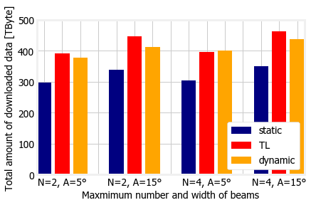
Figure 9: Total amount of downloaded data for different strategies and beam configurations, (i.e., maximum number of beams, beam half-power width).

The first aspect we are interested in is the performance of the proposed TL strategy against the optimum. Due to the problem complexity, the latter is found via brute-force, and, to make the brute-force approach terminate in a reasonable amount of time, we limit the comparison to two gNBs, namely, the two that in the topology in Fig. 1 are closest to each other.

Tab. VII presents the total amount of data that the vehicular users download under the TL and optimum strategies, and accounting for the actual channel conditions the users experience. We observe that TL is remarkably close to the optimum; furthermore, the difference is more significant in four-beam scenarios than in two-beam ones. This is due to the fact that, in some four-beam configuration, under TL the same vehicle may be served by multiple beams, which does not happen under the optimal strategy.

We also investigate the performance of TL in the full Luxemburg City scenario and compare it against the other strategies discussed in Sec. V-B. These results, shown in Fig. 9, have been obtained by considering again the actual channel conditions over time. As one might expect, more and/or wider beams consistently result in better performance. The comparison between different strategies is instead quite surprising. For all but one set-up, TL outperforms all other schemes, including Dynamic which uses real-time information (the reasons for this behavior are detailed next). As for Static, it performs fairly well in comparison to the alternatives, proving to be not only an interesting baseline but also a viable option when more sophisticated approaches are infeasible, e.g., when gNBs cannot be co-located with traffic lights.

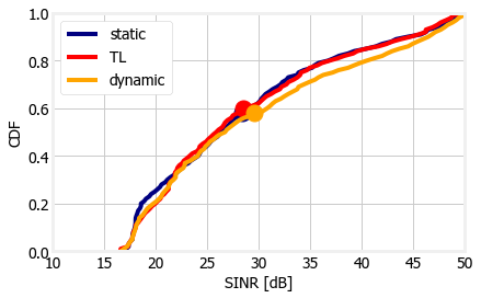
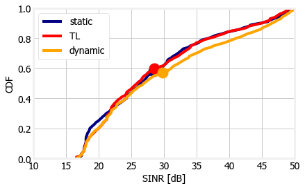
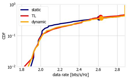
Figure 10: SINR experienced by served vehicles under different strategies, when there are: two beams (left) and four beams (right) with $A=5^{\circ}$. The average values are marked by a dot on each curve.

Figure 11: Actual rate experienced by served vehicles under different strategies, when there are: two beams (left) and four beams (right) with $A=5^{\circ}$. The average values are marked by a dot on each curve.

To understand where the difference in performance we observed in Fig. 9 comes from, we look at SINR and data rate achieved by the different strategies, summarized in Fig. 11 and Fig. 11, respectively. We can observe that Dynamic is able to achieve a better SINR than its alternatives; the average SINR value (marked by the dot in the curve) is around 2 dB higher for Dynamic than the other two strategies. This is thanks to the fact that beams can be steered exactly towards vehicles instead of towards road segments. Unsurprisingly, Static has the lowest SINR, owing to the fact that the direction of beams cannot change over time. There is another interesting effect we can observe when comparing Fig. 11 and Fig. 11. The Static strategy results in a slightly lower SINR for the vehicles experiencing worse conditions (the ones representing the worst 30% in the CDF curve), as we can see from the left part of the curves in Fig. 11. Such a difference corresponds, in Fig. 11, to a lower rate for those vehicles. The Dynamic strategy, on the other hand, provides the vehicles enjoying favourable propagation conditions with a substantially better SINR than its alternatives, as we can observe form the right part of the curves in Fig. 11. However, the difference in rate in Fig. 11 is much more limited; the average rate values, marked by the dots on the curves, almost coincide for the three different strategies. The reason is that SINR values are often so high that vehicles achieve the maximum possible rate, as shown by the jumps in Fig. 11: further increasing the SINR, as Dynamic does, brings little additional benefit. Comparing the left and right plots in Fig. 11 and Fig. 11, we can conclude that increasing the number of beams from 2 to 4, the system performance does not improve significantly.

The differences in SINR and actual rate shown in Fig. 11 and Fig. 11 do not fully explain, however, the performance difference displayed by Fig. 9. In Figs. 13 and 13, we therefore study for how long each vehicle is served under each strategy and the amount of downloaded data per vehicle. Recall that, in both figures, only served vehicles are considered. The difference between TL and its counterparts is now very clear and very significant. Under all set-ups, TL serves vehicles for a substantially longer time than the other strategies (Fig. 13) and, accordingly, it provides them with much more data. By comparing Fig. 13 to Fig. 13, we see that, although vehicles are served for virtually the same time by the Static and Dynamic strategies (Fig. 13), the latter results in a higher quantity of transferred data. In particular, there is an average increase of approximately $60$ Mbyte per vehicle;

this is a consequence of the difference in data rate we observed in Fig. 11.

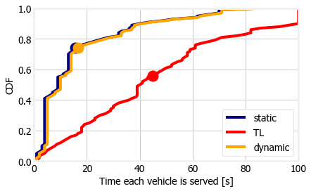
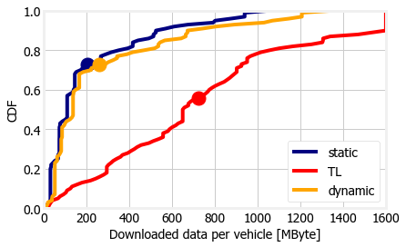
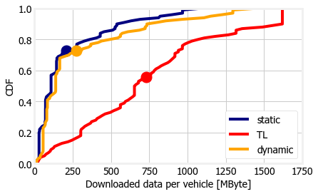
Figure 12: Time for which each vehicle is served under different strategies, for two beams (left) and four beams (right) with $A=5^{\circ}$. The average values are marked by a dot on each curve.

Figure 13: Data downloaded by each served vehicle under different strategies, when there are: two beams (left) and four beams (right) with $A=5^{\circ}$. The average values are marked by a dot on each curve.

The fact that vehicles are served for a much longer time under the TL strategy is consistent with the basic idea that TL should serve static vehicles waiting at a red light.

In summary, the TL strategy focuses on the vehicles that can profit the most from mmwave gNBs deployed at traffic lights, and provides them with as much data as possible for as long as possible. This may sound unfair; however, it is worth recalling that mmwave is not supposed to be the be-all and end-all of vehicular networks (or indeed, any kind of network). Mmwave is one of several technologies to be combined together in order to provide pervasive, high-capacity network coverage to mobile users, and using it to serve static users waiting at traffic lights is, in our scenario, the best way to make the most out of it.

VII Conclusions

Mmwave is a promising technology to enhance the capacity of vehicular networks. However, the performance of mmwave networks depends on the number, the alignment, and the width of beams between gNBs and vehicles, and these require knowledge of the vehicles’ mobility. Instead of relying on real-time mobility information, we proposed to rely on traffic signals, e.g., traffic lights, which influence the mobility itself. In particular, we first developed low-complexity approximate models for the mmwave channel gain and showed their accuracy in realistic scenarios, against more complex, existing models. Then we presented an optimization formulation for an effective beam design, and we proposed a low-complexity, heuristic solution, which proved to perform very close to the optimum.

Our performance evaluation, based on our innovative mmwave communication models and real-world topology and mobility information, has provided relevant insights. Leveraging traffic light-state information for beam design results in a network performance that exceeds that of baseline approaches (namely, static beam alignment) and is comparable to that of approaches using real-time mobility information.

References

- [1] S. Chen, J. Hu, Y. Shi, Y. Peng, J. Fang, R. Zhao, and L. Zhao, “Vehicle-to-everything (v2x) services supported by lte-based systems and 5g,” IEEE Comm. Standards Mag., 2017.
- [2] A. Bazzi, B. M. Masini, A. Zanella, and I. Thibault, “Beaconing from connected vehicles: Ieee 802.11 p vs. lte-v2v,” in IEEE PIMRC, 2016.
- [3] J. Choi, V. Va, N. Gonzalez-Prelcic, R. Daniels, C. R. Bhat, and R. W. Heath, “Millimeter-wave vehicular communication to support massive automotive sensing,” IEEE Comm. Mag., 2016.
- [4] M. Giordani, M. Polese, A. Roy, D. Castor, and M. Zorzi, “A tutorial on beam management for 3gpp nr at mmwave frequencies,” IEEE Communications Surveys & Tutorials, 2019.
- [5] H. Song, X. Fang, L. Yan, and Y. Fang, “Control/user plane decoupled architecture utilizing unlicensed bands in lte systems,” IEEE Wireless Communications, 2017.
- [6] T. Ba and R. W. Heath, “Coverage and rate analysis for millimeter-wave cellular networks,” IEEE Trans. on Wireless Comm., 2015.
- [7] H. Song, X. Fang, and Y. Fang, “Millimeter-wave network architectures for future high-speed railway comm unications: Challenges and solutions,” IEEE Wireless Communications, 2016.
- [8] J. G. Andrews, T. Bai, M. N. Kulkarni, A. Alkhateeb, A. K. Gupta, and R. W. Heath, “Modeling and analyzing millimeter wave cellular systems,” IEEE Trans. on Comm., 2017.
- [9] M. R. Akdeniz, Y. Liu, M. K. Samimi, S. Sun, S. Rangan, T. S. Rappaport, and E. Erkip, “Millimeter wave channel modeling and cellular capacity evaluation,” IEEE JSAC, 2014.
- [10] T. S. Rappaport, G. R. MacCartney, M. K. Samimi, and S. Sun, “Wideband millimeter-wave propagation measurements and channel models for future wireless communication system design,” IEEE Trans. on Comm., 2015.
- [11] 3GPP, “5G; Study on channel model for frequencies from 0.5 to 100 GHz - Release 14,” 3rd Generation Partnership Project (3GPP), Tech. Rep. 38.901, 2017.
- [12] M. Rebato, J. Park, P. Popovski, E. De Carvalho, and M. Zorzi, “Stochastic geometric coverage analysis in mmwave cellular networks with realistic channel and antenna radiation models,” IEEE Trans. on Comm., 2019.
- [13] M. Giordani, A. Zanella, and M. Zorzi, “Millimeter wave communication in vehicular networks: Challenges and opportunities,” in IEEE MOCAST, 2017.
- [14] L. Wei, Q. Li, and G. Wu, “Exhaustive, iterative and hybrid initial access techniques in mmwave communications,” in IEEE WCNC, 2017.
- [15] C. Perfecto, J. Del Ser, and M. Bennis, “Millimeter-wave v2v communications: Distributed association and beam alignment,” IEEE JSAC, 2017.
- [16] I. Filippini, V. Sciancalepore, F. Devoti, and A. Capone, “Fast Cell Discovery in mm-wave 5G Networks with Context Information,” IEEE Trans. on Mobile Computing, 2017.
- [17] M. Giordani, M. Mezzavilla, and M. Zorzi, “Initial access in 5g mmwave cellular networks,” IEEE Comm. Mag., 2016.
- [18] T. Nitsche, A. B. Flores, E. W. Knightly, and J. Widmer, “Steering with Eyes Closed: mm-Wave Beam Steering without In-Band Measurement,” in IEEE INFOCOM, 2015.
- [19] V. Va, T. Shimizu, G. Bansal, and R. W. Heath Jr., “Beaconing from connected vehicles: Ieee 802.11 p vs. lte-v2v,” in IEEE ICC, 2016.
- [20] A. Ali, N. Gonzalez-Prelcic, R. W. Heath Jr., and A. Ghosh, “Leveraging sensing at the infrastructure for mmwave communication,” arXiv, 2019.
- [21] V. Va, J. Choi, T. Shimizu, G. Bansal, and R. W. Heath Jr., “Inverse multipath fingerprinting for millimeter wave v2i beam alignment,” arXiv [https://arxiv.org/abs/1911.09796], 2019.
- [22] A. Loch, A. Asadi, G. H. Sim, J. Widmer, and M. Hollick, “mm-Wave on Wheels: Practical 60 GHz Vehicular Communication Without Beam Training,” IEEE COMSNETS, 2017.
- [23] Z. Limani Fazliu, F. Malandrino, and C. F. Chiasserini, “mmWave in vehicular networks: Leveraging traffic signals for beam design,” in IEEE WoWMoM Workshop on Communication, Computing, and Networking in Cyber Physical Systems (CCNCPS), 2019.
- [24] L. Codeca, R. Frank, S. Faye, and T. Engel, “Luxembourg sumo traffic (LuST) scenario: Traffic demand evaluation,” IEEE Intelligent Transportation Systems Magazine, 2017.
- [25] A. Schrijver, Theory of linear and integer programming. John Wiley & Sons, 1998.
- [26] E. M. Voorhees, “Implementing agglomerative hierarchic clustering algorithms for use in document retrieval,” Cornell University, Tech. Rep., 1986.
- [27] B. Antonescu, M. T. Moayyed, and S. Basagni, “mmwave channel propagation modeling for v2x communication systems,” in IEEE PIMRC, Oct 2017.
- [28] 3GPP, “Study on New Radio (NR) Access Technology – Physical Layer Aspects – Release 14,” 3rd Generation Partnership Project (3GPP), Tech. Rep. 38.802, 2017.
- [29] ——, “Evolved Universal Terrestrial Radio Access (E-UTRA) – Physical layer procedures – Release 15,” 3rd Generation Partnership Project (3GPP), Tech. Rep. 36.213, 2018.
- [30] M. Mezzavilla, M. Miozzo, M. Rossi, N. Baldo, and M. Zorzi, “A lightweight and accurate link abstraction model for the simulation of lte networks in ns-3,” in ACM Conference on Modeling, Analysis and Simulation of Wireless and Mobile Systems, 2012, pp. 55–60.