Singularities and vanishing cycles in number theory over function fields
Abstract.
This article is an overview of the vanishing cycles method in number theory over function fields. We first explain how this works in detail in a toy example, and then give three examples which are relevant to current research. The focus will be a general explanation of which sorts of problems this method can be applied to.
1. Introduction
This article concerns number theory over function fields - the study of classical problems in number theory, transposed to the function field setting. These proposed problems are then amenable to attack by topological, and more precisely cohomological, methods. The goal of this article is to give a broad, conceptual introduction to a specific set of topological techniques that have proven useful to recent works in this area. We begin with a brief review of the general study of function field number theory, though we recommend that anyone unfamiliar with it read another article on the subject (e.g. [12], [6]) before tackling this one
1.1. Number theory over function fields
We start by expressing a problem in number theory as the problem of finding an approximate formula (or proving an already conjectured one) for the number of elements in a fixed set. Many problems in analytic number theory and arithmetic statistics have this form, or can be reduced to it. For instance, a solution to the twin primes conjecture on the infinitude of twin primes would follow from a counting formula for the number of twin primes at most , for an arbitrary integer .
If this problem seems intractable, we can consider a finite field analogue, which may be easier. We take the definition of the set we wish to count and modify it by replacing each occurrence of the integers in the definition with the ring of polynomials over a finite field, but otherwise change it as little as possible. For instance, we could replace twin primes (numbers such that and are prime) with polynomials such that and are both irreducible polynomials. (More generally, if our problem involves the ring of integers of a number field, we can replace it with the ring of functions on an affine algebraic curve over .)
We can almost always recognize this new set as the set of points of an algebraic variety defined over , i.e. the solutions in of some finite list of polynomial equations, possibly after removing the solutions to another list of polynomial equations. The Grothendieck-Lefschetz fixed-point formula then gives an approximate formula for the number of points in this new set if we can calculate the (high-degree, compactly-supported, étale) cohomology of this algebraic variety.
If we don’t know how to calculate this cohomology, we could transfer the problem to yet another setting. We can consider the analogous, purely topological problem, of calculating the (high-degree, compactly-supported, singular) cohomology of the space of solutions in to the same list of polynomial equations. This can be attacked using any of the many known topological methods for computing cohomology groups. Once this is done, we can sometimes transfer back to the original finite field problem using comparison results for cohomology, or by using finite field analogues of our topological techniques. However, it is rarely possible to go all the way back and solve the original number theory problem by this approach.
1.2. The topological methods
This article will primarily discuss a cluster of methods useful in the last step - the application of topological tools to calculate cohomology groups. This cluster centers around vanishing cycles, and depending on the problem may also involve perverse sheaves, the characteristic cycle, and the search for suitable compactifications. We will focus mainly on vanishing cycles, but mention the others, because they seem to be closely related. These methods arose mainly from the study of the topology of algebraic varieties over the complex numbers - for instance vanishing cycles arose in the work of Lefschetz, and perverse sheaves arose in the work of Goresky and Macpherson [17]. They were then later applied to the study of varieties over finite fields as well - vanishing cycles by the SGA authors [18], and perverse sheaves by Beilinson, Bernstein, Deligne, and Gabber [3].
1.3. Comparison with homological stabilization theory
Before discussing these tools, we will compare them to homological stabilization theory - a different set of tools that can be used to tackle similar problems. In particular, the brilliant papers [13] and [14] reduced two number-theoretic problems over function fields to calculating the cohomology of certain Hurwitz spaces, and used tools from stable cohomology to make great progress on understanding, though not to completely compute, these cohomology groups.
In view of the philosophy that the most helpful information a paper can contain is an explanation of when the other information in the paper will be useful, let us discuss the situations when these two methods can be applied. Homological stabilization theory seems to be most effective when the space we wish to study have the following properties:
Desiderata 1.1.
-
(1)
is a manifold. In particular, we can use Poincaré duality to express the (high-degree) compactly supported cohomology of in terms of the (low-degree) usual cohomology.
-
(2)
has a nice descriptions as a classifying space of groups. For instance, may be a configuration space, a moduli space of curves, or a cover of one of these.
For example, the Hurwitz spaces studied in [13] and [14] are certainly manifolds, and moreover are covering spaces of configuration spaces. Thus, they (or their connected components) can be described as the classifying spaces of certain explicit subgroups of the braid group. On the other hand, the spaces discussed in this paper share a contrasting set of properties:
Desiderata 1.2.
-
(1)
is not a manifold - instead, it has singularities.
-
(2)
has a nice description as the set of solutions of a system of polynomial equations (e.g. it is described by simple equations, or equations of low degree, or relatively few equations, or all of these at once.)
-
(3)
does not have any obvious nice descriptions in terms of configuration spaces, moduli spaces of curves, etc.
-
(4)
lies in a natural family of spaces , depending on some auxiliary parameters . All the spaces in this family are defined by similar equations, but may have very different singularities. A generic member of the family often has no singularities at all.
Because homological stabilization was developed to study the usual cohomology of classifying spaces of groups, and is best adapted for this situation, conditions (1) and (3) are problematic if we wish to apply methods from that field.
More subtly, condition (4) is also problematic for methods from the field of homological stabilization or other purely topological approaches. If our spaces lie in a parametric family of different spaces, which are not all homeomorphic, then they are unlikely to have any nice purely topological description, even a non-obvious one. This is because topological constructions usually don’t depend on continuous auxiliary parameters in a nontrivial way. Instead, topological objects are invariant under continuous deformations.
On the other hand, for the methods discussed in this paper, not being a classifying space is not a problem, singularities can be dealt with, and (2) and (4) are both very helpful.
1.4. Contents
This article will begin, in Section 2, with a conceptual introduction to vanishing cycles theory that examines how it can be applied to a simple toy problem. (Some introductions with a greater level of technical detail include, in complex geometry, [26], and in the -adic setting, [15, §3] and [16, §9.2].) We will then move on to discussing three specific problems from recent research. We will explain the number-theoretic motivation, the spaces whose topology must be studied, and how they are related. We will then discuss how the spaces realize the properties (1)-(4) and how vanishing cycles, and related methods, have been used to attack them.
In number-theoretic terms, the problems we discuss will be
-
•
The moments of -functions. (Section 3)
-
•
The values of character sums over intervals. (Section 4)
-
•
The distribution of CM points on . (Section 5)
We do not assume familiarity with these problems in their classical, finite field, or topological incarnations.
1.5. Conclusion
A secondary purpose of this article is to be a survey of the great diversity of spaces whose cohomology is of interest in analytic number theory. In particular, many seem to arise from different fields of math. Some, such as the Hurwitz spaces, are perhaps most naturally defined topologically. Others, such as spaces of tuples of polynomials satisfying a congruence condition (discussed in §3), clearly hail from the world of algebraic geometry. Spaces defined using the Jacobian variety and Abel-Jacobi map (see §5), might be said to appear most naturally in complex geometry. The complements of hyperplane arrangements (§4) are quite natural from the perspective of all these fields. It seems reasonable to believe that the greatest progress in function field number theory in the future will come from combining vanishing cycles techniques, other topological techniques, and number-theoretic techniques to achieve something none of them could alone.
1.6. Acknowledgments
This article was written while the author served as a Clay Research Fellow. I would like to thank Johan de Jong, Jordan Ellenberg, Philippe Michel, and (especially) the anonymous referee for many helpful comments on earlier versions of this paper.
2. Vanishing cycles
Vanishing cycles originally arose in the context where we have a map of algebraic varieties over the complex numbers (or in topological language ) and view the inverse images of (or ) as a parametric family of varieties. When is smooth and proper, the fibers are compact manifolds, and moreover are all homeomorphic because we can flow one fiber into another using Ehresmann’s lemma. Thus, they have the same cohomology. Vanishing cycles theory is designed to study how the cohomology differs when this does not hold, and in particular the fibers are not all smooth.
2.1. A family of elliptic curves
To see how this theory works, let us consider the family of elliptic curves in with affine equation
| (2.1) |
Remark 2.1.
Taking the solutions to this equation in the projective plane involves considering the homogenized equation . Here we have added powers of to each term so that they all have the maximal degree. We then consider the space of solutions of this equation, with not all , up to scaling .
This has the effect of adding to the original solutions, which correspond to triples with , a new point “at infinity”. For general algebraic varieties, we may need to add more than one point at infinity, when there are multiple solutions with of the defining equations.
Remark 2.2.
We have chosen the examples in this section so that nothing interesting happens with the points at infinity, and they can safely be ignored, but dealing with these points can be an important difficulty in research problems.
The derivatives of the polynomial in the and variables respectively are and . The only points in the plane where these both vanish are and . Thus, the only points where this polynomial and its derivatives all vanish are and . Thus by the implicit function theorem, for , the solutions of this polynomial form a smooth manifold of complex dimension one - a Riemann surface. Because this equation has degree , the surface is an elliptic curve, i.e. a Riemann surface of genus one. (We will verify this formally in (2.8).) Therefore we can calculate the singular cohomology groups
| (2.2) |
for (i.e. for generic values of ).
On the other hand, for , the equation (2.1) has a singularity at the point , and is not smooth. To understand its topology, we can use its parameterization - solutions can be written for . In fact, projective solutions to (2.1) can be given by the same formula for in the Riemann sphere.
Remark 2.3.
To find this parameterization, one can set and then solve for and in terms of .
Because , this parameterization is one-to-one, except for when and are both , which occurs for and . It follows that the solution set to (2.1) with is obtained from the Riemann sphere by gluing together the two points and . From this description it is easy to compute its cohomology as
| (2.3) |
(perhaps most easily by giving it a CW complex structure with one -cell, one -cell, and one -cell.)
The vanishing cycles method explains the discrepancy between (2.2) and (2.3) using local information at the singular point .
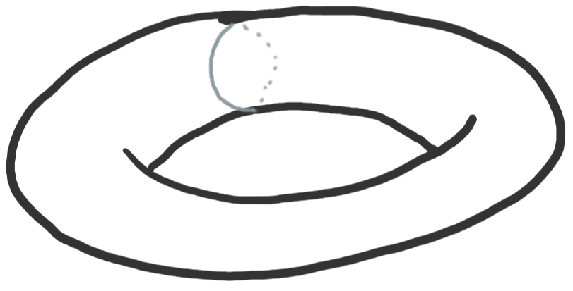
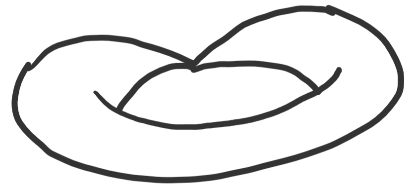
Given any cycle in the homology of , as goes to we can continually push the cycle into a new fiber, producing a cycle in . If were smooth, this map would give an isomorphism on homology. However, where there is a singularity something else can happen - a nontrivial cycle in can collapse down to a single point in . This happens precisely for one nontrivial circle around the torus. In fact, taking a circle on a torus and collapsing it down to a single point produces a space which is homeomorphic to a sphere with two points glued together. as in Figure 1.
2.2. Generalities on vanishing cycles
More generally, the classical vanishing cycle theory shows, when is a parametric family of complex spaces where is smooth for all but finitely many and has isolated singularities, that:
-
•
There is a natural map , for generic near .
-
•
This map fits into a long exact sequence, whose third term is a sum of contributions from singular points.
-
•
The contribution of each singular point depends only on local data in a neighborhood of this point - more precisely, it is the reduced homology of the Milnor fiber.
In the arithmetic setting, it is most convenient to express this data using sheaf cohomology:
Properties 2.4.
-
•
There exists a map , for the generic value of .
-
•
This map fits into a long exact sequence, whose third term is the cohomology on of a complex of vanishing cycles .
-
•
is supported at the singularities of .
-
•
is defined locally, so its stalk at a point depends only on the geometry of and in a neighborhood of that point.
If the singularities of are isolated, then is by definition the sum over the singular points of of the stalk of at that point, and this recovers the cohomological dual of the classical picture. If there are higher-dimensional singularities, then cohomology of the complex is a more complicated operation.
For now, let us focus on the case where singularities are isolated. In particular, we will show how, using only these facts, and not knowing anything else about the definition of vanishing cycles or elliptic curves, one can recover the cohomology of the family described by (2.1). This fits with how vanishing cycles arguments in the arithmetic setting usually proceed in practice - it’s usually most convenient to use abstract properties as much as possible and definitions and constructions as little as possible.
Remark 2.5.
For precision, we will state the definition of vanishing cycles in a general context. Let be a variety with a map . Let be the fiber of over and let be the inclusion. Let be a small disc around . Let be the universal cover of the punctured disc . Let and let be the projection map.
There are pullback and derived pushforward functors, and respectively, associated to , and an adjunction map . Applying the pullback functor we obtain a map , whose mapping cone is defined to be .
From this definition the claims of Properties 2.4 can be deduced: From the definition of the mapping cone we have a long exact sequence
We have so the first term is , and one can check that the second term is using the proper base change theorem. Because of the smooth base change theorem, vanishes away from singularities, and because both and the adjunction can be defined locally, the vanishing cycles can be defined locally.
2.3. A family of conics
To understand the cohomology of the family from §2.1, we will compare to a simpler family , defined by the equation
| (2.4) |
or equivalently
| (2.5) |
Homogenizing this equation, we get , which when has two nonzero solutions, and , up to scaling. Thus the projectivization of this family has two additional points at infinity.
For , we can parameterize the solutions of this equation by setting , so and thus
Here and go to the two points at infinity. This map shows that the solution set is isomorphic to the Riemann sphere, and thus
| (2.6) |
for . On the other hand, if , the solution set consists of two Riemann spheres, with and respectively, glued at the point . The cohomology of two spheres glued at a point can be calculated as
| (2.7) |
by using a CW complex with one -cell and two -cells.
We now consider the vanishing cycles long exact sequence associated to this family, for a generic value of :
which specializes to
To calculate this long exact sequence completely, it suffices to check that the maps and are surjective. In the classical setting, we would check that flowing the corresponding homology cycles - either a point or all of - from to produces a nonzero cycle, in this case either a point or all of . In an arithmetic setting, it might be more straightforward to check from general vanishing results that vanishes in degrees and , so .
From this long exact sequence, we now obtain
Recalling that in the case of isolated singularities, this cohomology is a fancy notation for a sum over the singular points, we conclude that the contribution of the singularity is in degree .
2.4. Comparing the two families
Now comes the key point: A neighborhood of the singularity in the solution set of the equation (2.4) is isomorphic to a neighborhood of the singularity of the equation (2.1), under the map that fixes and and sends to . Thus, the vanishing cycles contributions of that point to the two different families must be identical. Furthermore, in there are no other singularities that contribute, so we must also have
Thus, the vanishing cycles long exact sequence
using this equation and the calculation (2.3) of the cohomology of the special fiber, reduces to
Using the the fact that is a compact surface and so , we can see that the map into is nonzero, which determines all the other maps and in particular forces
| (2.8) |
Thus, we have verified (2.2). By the classification of oriented surfaces, we can confirm that must be a surface of genus one.
Of course, there are easier ways to check that is topologically a torus. But there are other problems where the vanishing cycles strategy demonstrated here is essential. We can find a nice family of spaces, and try to deduce facts about a particular fiber from knowledge about the general fiber, or, as in this case, deduce facts about the generic fiber from information about a particular one. It suffices to find all singularities of this particular fiber and estimate their vanishing cycles contribution. To do this we can look at a small neighborhood of the singularity and try to understand its geometry. In particular, we could find another family of spaces, defined by a simpler equation, with a singularity of the same type - ideally as its only singularity. Finally, we can reduce the vanishing cycles question to a global question about this simpler space. Hopefully, we can solve this problem directly. By reducing a global question on our original family to a local question at a singularity to a global question on a new family, we have progressively simplified the problem, eventually reaching a form that we know how to solve.
2.5. Calculating the monodromy
In addition to calculating the cohomology of the fibers , we can gain a little more information about the family using the same analysis of the singularity we did already. Suppose we send in a small circle around , and let vary. Because remains smooth for all these values, we can always flow into the next one. This flow defines a mapping class of homeomorphisms and thus a map on cohomology . This map is known as the monodromy action. Because it comes from an (orientation-preserving) homeomorphism, it certainly fixes and . How does it act on ?
It is a classical fact that, for this family and similar ones, the action is unipotent. Topologically, one can recognize this mapping class as a Dehn twist, which always acts by unipotent transvections on . A more number-theoretic argument would recognize this loop as a loop around a cusp in the modular curve parameterizing elliptic curves. The modular curve is a quotient of the upper half-plane by , with each loop defining a conjugacy class in , and the action on given by the standard representation of . From examining the geometry of the upper half-plane and this action, one sees that a loop around a cusp defines a unipotent conjugacy class.
Let us see how we can verify this same fact with vanishing cycles. The key facts are that
-
•
We can define a monodromy action on such that all the maps of the vanishing cycles long exact sequence commute with monodromy. Here we take monodromy to act trivially on .
-
•
This action on the contribution of a singularity depends only on the geometry of and in a neighborhood of that singularity.
Examining the vanishing cycles long exact sequence for the family of conics defined in §2.3, we see that is a subspace of . Hence, because it is a subspace of a space with trivial monodromy action, it has trivial monodromy action. Thus, in a short exact piece
of the vanishing cycles long exact sequence for , which reduces to
the monodromy action is trivial on both s. Hence the action on must be unipotent.
So we have recovered this unipotence phenomenon without needing any understanding of the surface . One could go further, and check that this monodromy action is nontrivial unipotent, using Deligne’s theory of weights, but this would take us too far afield.
2.6. Conclusion
The arguments we have just seen highlight some key properties of vanishing cycles theory, which should start to provide an explanation for Desiderata 1.2:
-
(1)
The singularities of the special fibers and did not harm our argument. Instead, they helped - the singularity of gave it a rational parameterization, making its cohomology easier to compute, which we could use, together with the family , to compute the cohomology of the more difficult smooth fiber .
-
(2)
The simplicity of the polynomial equation defining was a big help. It let us find the singularity, and once the singularity was found, suggested how to simplify the geometry by removing the few high-degree terms in the equation.
-
(3)
The fibers have a nice description as topological tori, and the family has a nice description as a cover of the moduli space of elliptic curves, but we did not use either of these.
-
(4)
It was absolutely crucial that we were studying a family , and not just a single Riemann surface. The fact that the generic member was smooth was also helpful.
Let us also mention two more technical points about using vanishing cycles in general:
Remark 2.6.
Vanishing cycles theory is simplest when the singularities are isolated, i.e. the singular locus has dimension . But even when the singularities are not isolated, it is better for the dimension of the singular locus to be smaller. This is especially crucial because of what we know about the degree of the vanishing cycle complex, which in general is a complex of sheaves and not just a sheaf. It was proven in [18, I, Corollary 4.3] that has a property that was later called semiperversity - its ’th cohomology sheaf is supported in a set of dimension . Because any sheaf on an algebraic variety of dimension has cohomology in degree at most , this implies that vanishes unless
which combined with the spectral sequence
implies that vanishes unless
where is the singular locus of . This vanishing was used to great effect in [20, appendix by Katz]. Even when vanishing is not enough and more precise control of the vanishing cycles is needed, this is generally easier to achieve when the dimension of the singular locus is smaller. Finding an interesting space whose singular locus is unexpectedly small can itself represent substantial progress towards the solution of an arithmetic problem.
Remark 2.7.
It is required for the vanishing cycles exact sequence to hold that the map be proper, as otherwise a cycle could escape off to infinity, which would not be explained by any data locally in the fiber. Thus, to apply this method to noncompact spaces, it is necessary to compactify by adding additional points, usually taking the form of a “boundary divisor” or “divisor at infinity”. Then one has to control the vanishing cycles for points at this divisor over the special fiber as well, and it is crucial to choose a compactification where this can be done.
3. Statistics of -functions
We begin this section with a brief precise statement of the question we will consider, before explaining in more detail the motivation behind it in §3.1, and then finally studying it as a topological problem in §3.2. We will see that vanishing cycles can solve important special cases of this problem, but not yet the full problem - something that future work will hopefully be able to rectify.
Let be a field (either finite or the complex numbers), a polynomial of degree over , a natural number, and additional natural numbers.
Let be the set of tuples of polynomials over , with monic of degree , where and share no common factors, and where
Some natural number-theoretic problems over reduce to counting the elements in . This motivates us to consider the analogous question of calculating the compactly-supported cohomology of (given its natural topology as a subspace of the space parameterizing tuples of monic polynomials of degree ).
3.1. Background and motivation
Fix a finite field and polynomial ring in one variable over that finite field. Let be a polynomial. We have the quotient ring and its group of invertible elements . The class in of a polynomial is invertible if and only if .
For a character, we can form the Dirichlet -function
This is a close analogue of the usual Dirichlet -function studied over the integers, which for and is
Here we think of the positive condition and monic condition as being analogous, and the terms and terms as being analogous.
Remark 3.1.
We can make the second analogy more clear by setting , so , and noting that for an integer , is the cardinality of the quotient ring , so we should define to be the cardinality of the quotient ring , which is . However, substituting for would make our formulas slightly more complicated, so we avoid it for the rest of this argument.
A key fact about is that it is almost always a polynomial in :
Lemma 3.2.
Fix of degree and a nontrivial character. Then is a polynomial in of degree .
Proof.
It suffices to prove that the coefficient
of in vanishes for . To do this, note that when , any residue class in occurs for exactly monic polynomials of degree . Indeed we can represent any class in by a polynomial of degree , and then add the product of by any monic polynomial of degree to find such an . Because there are monic polynomials of degree , we have choices for . So the coefficient of in equals
However,
because the sum of any nontrivial character over the elements of a group vanishes. So the coefficient equals zero, as desired. ∎
In fact, Weil proved [36]:
Theorem 3.3.
Fix of degree and a character. Assume that
-
(1)
There does not exist a polynomial of degree dividing such that depends only on the congruence class of modulo .
-
(2)
The restriction of to is a nontrivial character of .
Then is a polynomial in of degree , with all roots satisfying .
Remark 3.4.
Weil proved that the roots satisfy as a special case of his Riemann hypothesis for curves over finite fields. The strategy is similar to the classical argument in number theory that writes the Dedekind zeta function of a cyclotomic field as a product of Dirichlet -functions, so that the Riemann hypothesis for zeta functions of cyclotomic fields would imply the Riemann hypothesis for -functions of characters. The function fields of the curves used in this proof are analogues of the cyclotomic fields, which can be defined using the Carlitz module or using explicit equations similar to (4.3) below.
Remark 3.5.
Under assumption (1), we say that is primitive, and under assumption (2), we say that is odd.
Remark 3.6.
When the character is not primitive and odd, there is always a simple way to modify to obtain a polynomial, of degree , with all roots satisfying , by removing certain trivial zeroes which are roots of absolute value .
When the character is not primitive, this can be achieved by simply replacing with the polynomial discussed in assumption (1), which is why it is usually fine to restrict attention to the case of primitive characters.
Theorem 3.3 is expected to be essentially the strongest result that is true about all - in other words, any polynomial of degree with all roots on the circle of radius could well appear as some . (If we allow the parameter to go to , a precise version of this expectation is known to be true in the case where is squarefree [22].) Thus, when we study these -functions after Weil, we usually study them in a statistical manner - we wish to know how the roots or values of this -function behave, as random variables, when we select uniformly at random from the set of all characters (or all primitive odd characters - we will ignore this technical distinction.)
One fundamental statistical question about the -function are its moments, or more precisely, the moments of its values at a particular point.
Question 3.7.
For of degree and , what is
This question is considered most interesting when , because for larger, respectively smaller, values of , the high degree, respectively low degree terms dominate , making the problem simpler.
This question, and its variants, have been heavily studied in number theory over the integers, and studied, though not as heavily, in the setting of . Precise formulas predicting the value of this moment in the limit as goes to have been conjectured [7, 1], but they are known to hold only for and (and in the case, the proven bounds on the error term are much worse than the expected bounds, so more progress is possible there).
We can convert this moment problem to a counting problem by using the definition of to write
(Technically, the sum over is divergent when is the trivial character because has a pole, and so one should subtract that term off before exchanging the order of summation. We will ignore this issue to simplify our formulas and focus on the most important steps. We could instead restrict the sum to primitive odd characters using a suitable inclusion-exclusion, but the main difficulty would still be the same.)
Using orthogonality of characters, one deduces that
so we conclude that
To calculate this, it suffices to estimate
| (3.1) |
In fact we need only estimate this for as if there will be exactly possible values of in each residue class mod , which will simplify (3.1) to an explicit formula which we can sum as a geometric series. (Or we can view these terms as the contribution of the trivial character and subtract them off.)
The estimate we seek for (3.1) will consist of a main term given as an explicit function of and an error term which is unknown but bounded by an explicit function in . We then sum both terms over from to to get an explicit estimate for the moment of . (This sum, because its length is relatively short, is much easier than the sum defining (3.1), which we expect to provide the main difficulty.)
Next, we can express as the solution to a system of equations over , minus the solutions of another system of polynomial equations.
First, we describe the set of tuples of monic polynomials over , with of degree . To do this, we need variables for the coefficients of each (other than the leading coefficient, which is fixed at ), for a total of variables.
Next, we express the condition that as a system of polynomial equations. The first step is to observe, that the coefficients of and are each polynomial functions of degree in the coefficients of the , which we have chosen to be our variables. To check if and are congruent mod , we divide each of them by and then take the remainder, using polynomial long division. Examining the polynomial long division algorithm, one can see that the coefficients of these remainders are respectively linear functions in the coefficients of and , and thus are polynomial functions in the coefficients of the . Equating the two remainders is equivalent to equating each of their coefficients, and thus it defines polynomial equations in the coefficients of the .
Finally, we express the condition as the negation of another system of polynomial equations. To do this, note that it is equivalent to asking that, for each prime polynomial dividing , . Again using polynomial long division, we can express as a system of equations in the coefficients of . (Another approach is to use polynomial resultants.)
Thus, we have described as the -points of an algebraic variety . Therefore, general principles (i.e. the Grothendieck-Lefschetz fixed point formula) allow us to reduce the problem of counting to calculating the cohomology . This motivates our study of the analogous cohomology problem over the complex numbers.
3.2. The space over
Let us now assume that the base field is the complex numbers.
In this case, our description of can be simplified. Because is a polynomial of degree , it has exactly roots, counted with multiplicity. Let be these roots. Assume for simplicity that these roots are distinct. A polynomial is a multiple of if and only if its value at each of these roots vanishes, so two polynomials are congruent mod if and only if they have the same value at each of these roots. Thus we can re-write the definition of as follows:
Let be the space of tuples of monic polynomials with coefficients in , such that , for all from to and from to , and for all from to .
In this case, we have .
We want to study the cohomology with compact supports .
Let us see why this space satisfies the properties of Desiderata 1.2.
-
(1)
can admit singularities. By definition, the singularities are the points where the Jacobian matrix of the system of polynomials , for to , does not have the maximum possible rank . (This definition is justified by the fact that these will be the points where the implicit function theorem does not force to be a manifold.)
With this definition in hand, finding the singularities is an elementary problem of polynomial algebra. We will see later in Lemma 3.8 that as soon as , a point is singular if and only if there exists a polynomial , of degree , such that is a polynomial multiple of for all .
An interesting point about these singularities is that they do not seem to appear in the number-theoretic analysis of this problem - none of the analytic tools that are used to attack the moments of -functions suggest that the case where the variables all divide some number which is not too large is particularly special. They singularities only become visible when we first transfer to the function field setting and then interpret geometrically.
-
(2)
We see from our explicit description that is the solution set of equations of degree in variables, minus the solutions of linear equations. These numbers are all relatively small - for some interesting spaces, our degrees or quantities of equations grow exponentially in terms of our parameters of interest, and this is much better. Moreover, the individual equations can be expressed nicely in terms of polynomials, which helps us do things like give a precise description of the singular locus.
-
(3)
While the space of all monic polynomials of degree with for from to has a nice description as a configuration space of points, which may collide, on , the condition that does not seem to have any meaning in terms of configuration spaces, and thus there is no known purely topological description.
-
(4)
We can deform to a family of similar, but distinct spaces by varying the defining equations slightly. More precisely, we can deform the equations into equations for . Doing this has a dramatic effect on the singularities. In fact, one can check that for generic choices of , there are no singularities at all, as the dimension of the space of possible in Lemma 3.8 is less than the dimension of the space of possible tuples .
We can also vary the roots . However, varying the roots does not change the singularities much, and so varying seems most useful for vanishing cycles theory.
Let us now check our characterization of these singularities, which is essentially due to Hast and Matei [19].
Lemma 3.8.
Assume that . Let be a point of . Then is a singular point of if and only if there exists an auxiliary polynomial , of degree , which the all divide.
Proof.
By definition, is a singular point if and only if the Jacobian matrix of the system of polynomials for from to has rank less than its maximum value, which is .
Let us first check that if such an exists, then is singular. To do this, we use the fact that the image of the Jacobian matrix consists of the derivatives of this tuple of polynomials along every path in starting at . We can view this path as as a one-parameter family of polynomials in an additional variable , where . Then the derivative along this path is
We are interested in taking the derivative at a point which lies in so we may assume that the equations are actually satisfied at , which causes the derivative at to simplify to
| (3.2) |
Now each term is a rational function in that vanishes at (because the leading coefficient of each is fixed at ) and whose denominator divides (by assumption). Hence
is a rational function in that vanishes at and whose denominator divides . Because this rational function vanishes at , the degree of its numerator is strictly less than the degree of its denominator, which is at most because it divides . So the numerator of this sum is a polynomial degree . There are only linearly independent polynomials of degree . Thus for different one-parameter families with the same , we can obtain at most linearly independent tuples
Thus, the image of the Jacobian matrix has dimension at most , and it does not have full rank.
Conversely, suppose the Jacobian does not have full rank. Then there is a linear combination of the derivatives (3.2) which vanishes for all families . Thus there exist constants such that
By Lagrange interpolation, a polynomial of degree is uniquely determined by its values on , so there exist constants such that the coefficient of in is . Furthermore because there exists a degree polynomial vanishing on . Then for each we can find, by Lagrange interpolation again, a polynomial of degree such that .
Now can be an arbitrary polynomial of degree . It follows that for all polynomials of degree ,
It follows that if , then the coefficient of in vanishes, so . Applying this for , we show that , so we can apply it for , showing , and so on, until we apply it for , and show .
Now has degree , so is determined by its values at , which are and in particular are independent of . Hence is equal to a fixed polynomial of degree for all . Thus all the divide , as desired.
∎
However, we do not know how to apply the vanishing cycles method, or other similar methods, to for all values of . The reason is that the singularities are too big. For example:
Lemma 3.9.
Assume that for all from to . Then the dimension of the singular locus of is at least .
Proof.
For any monic polynomial of degree , we can choose to be an arbitrary divisor of this polynomial with degree and to equal , so that the equation is automatically satisfied. This point will be singular by Lemma 3.8. If , then we can choose to cover all the roots of . Having done this, we will obtain distinct tuples of polynomials for distinct , so the dimension of the singular locus is at least the dimension of the space of possible .
If , we can do the same thing with of degree . ∎
This dimension is large enough that we don’t obtain any estimates for the moments stronger than what can be obtained directly from the much easier Theorem 3.3, which implies and so the average of is at most .
However when is large and are small, or vice versa, the problem disappears. In fact, in the extreme case, the singularities are isolated.
Lemma 3.10.
Suppose . Then the singular locus of consists of finitely many points.
Proof.
Let be a singular point. We apply Lemma 3.8 to conclude that there exists an which all the divide. Let be the roots of .
Any monic dividing must have the form
for some , so
for some . By removing the root from in case , we may assume that all the are positive. There are finitely many possible values for the , and for each of them, the system of equations
has finitely many solutions.
To check this, it suffices to show that the Jacobian of this system of equations in variables has full rank. We calculate the Jacobian using logarithmic derivatives. This gives a matrix whose entries are which cannot have a kernel as, for a vector in the kernel, would be a nonzero rational function with poles, each of multiplicity one, and zeroes, vanishing at , which is impossible as .∎
Because the singularities are isolated, applying the vanishing cycles method to control the singularities of in the case looks promising. However, we are far from done with the problem at this point. To apply the method, we also need to compactify the variety, understand the singularities and vanishing cycles at the points at infinity of this compactification, bound the dimension of the vanishing cycles sheaf at each isolated singularity, and calculate the cohomology of the generic fiber.
All of these steps were carried out for a slight variant of this problem in [30]. In this variant, rather than demanding mod , we demand the coefficients of in vanish. This variant is almost the same as the case when , using the change of variables that reverses the order of the coefficients of a polynomial, but because monicity is not preserved by this change of variables it ends up relating to the moments of only those modulo with (i.e. the even characters).
This vanishing cycles argument in [30] concludes in showing that for all
where
that is one-dimensional, and that the dimensions of the cohomology groups in degrees are bounded by . Similar results, with a slightly weaker cohomology vanishing statement, were proved for -adic cohomology in characteristic .
Obtaining these results requires studying a compactification. A good choice involves embedding into the weighted projective space where the th coefficient of a polynomial is a coordinate of degree . This makes the coefficient of homogeneous of degree , so the equations defining are each homogeneous. (Alternatively, we can reduce to the case where each by factoring each into linear factors. In this case, our compactification embeds into an unweighted projective space.) A variant of Lemma 3.10 works in this setting, showing that the singularities of the compactification are isolated. (In characteristic , we can only give an upper bound on the dimension of the singular locus, which improves as grows). We can apply vanishing cycles in a family where we vary the defining equations of to the equations defining a smooth affine complete intersection. The analogous vanishing result for the cohomology of the affine complete intersection is well-known. Because the singularities are isolated, the vanishing cycles sheaf is supported at finitely many points, so its cohomology satisfies a similar vanishing result. By applying the vanishing cycles long exact sequence, we can conclude that for and is one-dimensional if .
Finally, the bounds for the dimension of the cohomology groups use a separate method of Katz which proves bounds for the cohomology groups of a variety in terms of the number of variables, number of defining equations, and degrees of defining equations [21].
By proving these results on cohomology, [30] was able to obtain estimates for sums of divisors functions, as well as a variant of Question 3.7 where the -function is not encased in an absolute value, i.e. an estimate for
To see why this estimate was obtained, note that following the arguments of §3.1 without the absolute value, we obtain the counting function in the special case where .
It is likely possible to carry out a similar argument for values of other than . In the case when has distinct roots, this will be done in [32]. Here a suitable compactification embeds into a product of projective spaces, where the coefficients of each are the coordinates of a different projective space. We can apply vanishing cycles in the family varying discussed above. In this case, the compactification adds new singularities, but their structure is so simple that we can explicitly check there are no vanishing cycles at these singular points. Here the cohomology of the generic fiber is much subtler to compute and requires a careful analysis of the compactification and the theory of perverse sheaves. The final result is a calculation of the compactly supported cohomology of in all degrees but and , and bounds on the dimensions of cohomology in those degrees (still in the case .) This again leads to estimates for moments without the absolute value, this time for characters modulo a squarefree polynomial .
3.3. Future work
It would be of great interest to generalize the vanishing cycles techniques to general polynomials which are neither squarefree not a power of , or to handle the case when is large for both and , even for very specific . For general , the main difficulty is finding a good compactification, but to handle the case where all are large, more ideas than that are necessary.
4. Short character sums
Many problems in analytic number theory involve, at a crucial point, short character sums. Let be a natural number and let be a homomorphism. Extend to a function on by setting if (and therefore is not an invertible element of ). Then a short sum of has the form
| (4.1) |
for and . Because is a finite group, takes values in complex numbers of modulus . Because each term has modulus at most , the size of this sum is at most the total number of terms, which is . Thus the trivial bound for this sum is
If is the trivial character, this bound is essentially sharp, but for any other , the trivial bound can often be improved. The most important improvements are the Pólya-Vinogradov inequality [28, 35]
which improves on the trivial bound for , and the Burgess bound [4], which is more complicated to state, but improves on the trivial bound whenever for any fixed . Bounds which improve on the trivial bound for a greater range of possible , or bounds which improve on it to a greater extent, would have numerous applications in analytic number theory.
It turns out that this problem has a very natural topological analogue, at least in the case when the modulus is squarefree, and this analogue can be almost completely solved. However, the translation between arithmetic and topology is nontrivial. Thus, we will explain the topological problem first, then explain the relationship with character sums, and finally explain what makes it solvable.
Let and be natural numbers. Let be a tuple of distinct complex numbers, and let be another tuple of complex numbers, not necessarily distinct. Let be the moduli space of polynomials of degree such that for from to .
Note that the space of polynomials of degree is simply , as we have one coordinate for each coefficient of the polynomial. Using these coordinates, is a linear function on , so the set of such that is a hyperplane in , and thus is the complement of hyperplanes in . So our space under consideration is a special type of hyperplane complement.
Question 4.1.
What is
where is a nontrivial one-dimensional representation of ?
In other words, we consider, not the usual cohomology, but cohomology twisted by some local system of rank on our space. Other than that, the situation is a standard one for arithmetic topology - our goal is to show vanishing of the high-degree compactly supported cohomology groups, or, equivalently (because Poincaré duality is valid in this setting), of the low-degree usual cohomology groups, as well as some reasonable bound for the dimensions of the middle groups.
4.1. The relation between topology and arithmetic
The first step in the translation to topology is to develop -analogues of every element of our arithmetic problem. We can replace with a monic polynomial . Let be the degree of .
We can then define as a homomorphism , and extend it by zero to non-invertible elements.
To find the appropriate analogue of an interval, we observe that the set of all with behaves like an interval around , in particular because it contains all polynomials whose norm is small, and thus the set of polynomials , where is fixed and varies over polynomials with , behaves like an interval around . Thus, the function field analogue of (4.1) is
| (4.2) |
However, it is equivalent, and will be more convenient later, remove the terms where is set to from the sum, obtaining
This will be convenient as it puts more of the complexity into the set we are summing over rather than the function being summed, and the set is easier to interpret geometrically.
For the trivial bound, we can observe that there are possible with , as each coefficient can take values, so we have
Again, the key problem is to substantially improve the trivial bound when is not the constant function .
To do this, we let for a monic polynomial and a polynomial , both over a field , be the set of polynomials over with and .
Over the complex numbers, we can factor . In this case, if and only if some factor divides , which happens exactly when , or . Thus, setting , the set of polynomials with is exactly the set where for all .
Hence is the topological analogue of the set we sum over in (4.2). We have thus translated every aspect of our arithmetic problem into topology, except for the character . Why should the analogue of summing the character be taking cohomology with coefficients in a representation of the fundamental group? The answer comes from the twisted Grothendieck-Lefschetz formula ([8, Rapport, Theorem 3.2] or [16, Theorem 10.5.1]).
For a space over a finite field , the usual Grothendieck-Lefschetz formula expresses in terms of the trace of a Frobenius element on the compactly-supported cohomology . The twisted Grothendieck-Lefschetz formula does the same thing for the cohomology , where is a representation of the fundamental group of . Because we are working in the finite field setting, it is necessary that we use the étale fundamental group . So let us take to be a representation of over .
For us, the crucial property of is that, for any covering space (technically, a finite étale map), and any , acts on the -points of the fiber of over . Furthermore, the isomorphism class of this fiber, as a set with a -action, is independent of . This is the analogue of the classical monodromy action on the fiber and its invariance under change of fiber. (More carefully, we need to pick a base point for the fundamental group, and then the action of the fundamental group on the fiber over another base point is well-defined only up to conjugacy, but our actions will factor through abelian groups so conjugacy is trivial and thus this detail is irrelevant.)
It turns out there are special conjugacy classes , for each , which are characterized by the property that the action of on a point is the same as the action of - in other words is the same as raising all coordinates of to their th power. The twisted Grothendieck-Lefschetz fixed point formula states
Thus, because we know that is exactly the set of we wish to sum over, to interpret (4.2) geometrically, it suffices to find a representation of such that .
To find such a representation, we use a strategy due to Lang [24, §3].
Let be the space with coordinates , which we view as the coefficients of a polynomial , and , which we view as coefficients of a polynomial , subject to the conditions
and
| (4.3) |
In particular, the important equation is the last one, because this “forces” to act by multiplication by . More precisely, this is a system of equations, one for each coefficient mod .
Let be the map that forgets and remembers . Lang [24] proved the key facts:
Theorem 4.2.
-
(1)
is a finite étale map, so is a covering space of .
-
(2)
acts on by fixing and acting by multiplication modulo on the polynomial .
-
(3)
This action is simply transitive on the fiber of over any point of defined over an algebraically closed field.
-
(4)
The action of each element of on a fiber of is equal to the action of some unique element of , defining a homomorphism .
-
(5)
The image of under this homomorphism, for a point , is .
Indeed our (1) is [24, discussion before Theorem 2 on p. 557], (2) and (3) are [24, (3) on p. 556], and (4) and (5) are the case of [24, (6) on p. 560], though all of these are expressed in different language.
Proof.
There are many things to check, and all can be done straightforwardly, so we just give a sketch, except for the most important ones.
For (1), the key point is that when differentiating the equation (4.3) with respect to , we can treat the terms as constant because the derivative of is a multiple of and thus vanishes.
For (2), the key point is that, because elements of are preserved by raising to the th power, when we multiply by a polynomial with coefficients in , we multiply on the left and right side of (4.3) by the same polynomial, and so (4.3) is preserved.
For (3), the key point is the reverse - the only elements of any field of characteristic preserved by raising to the th power are those in . When we divide two solutions of (4.3), with the same , by each other, we get a polynomial invariant under raising each coefficient to the th power, and this fact enables us to conclude that its coefficients are in .
(4) follows from (3) and some naturality properties of the action. This action is defined in an isomorphism-invariant way, which means that the action of any element of commutes with the action of any automorphism of fixing . But for a finite abelian group acting simply transitively on a finite set, the only permutations that commute with the action of are precisely the elements of .
(5) is the crux of the matter, because it is what allows us to explain why we chose the particular equation (4.3), rather than listing the miraculous properties of an equation which seemingly appeared out of nowhere. But it is also straightforward. We have defined the action of as by multiplication on modulo . We have also defined with . Thus, to guarantee that raising each coordinate to the th power is equivalent to multiplying by modulo , we need
which is precisely (4.3).
∎
It follows from Theorem 4.2 that if we compose this homomorphism with a one-dimensional representation of , we obtain a one-dimensional representation of such that , as desired.
The Grothendieck-Lefschetz formula now tells us how to express the sum of in terms of the compactly supported cohomology of . Because is smooth, we may as well consider the usual cohomology of , which is also a one-dimensional representation.
This explains why the complex analogue has cohomology twisted by a one-dimensional representation.
Remark 4.3.
A subtlety here is that the Grothendieck-Lefschetz formula applies over and we wish to study exponential sums over . To fix this we fix some isomorphism between the algebraic closure of and , which lets us freely transition between the two of them. To avoid using the axiom of choice, we could instead choose an isomorphism between some sufficiently large subfields of those fields. This technical detail almost never causes trouble and thus should be ignored whenever possible.
4.2. Topological methods
Let us now examine the spaces from the perspective of topology. There are multiple methods to studying the twisted cohomology of hyperplane complements that could be applied to - in the complex setting these include [5] and related works giving criteria for nonvanishing outside the middle degree. Here we will focus specifically on the approach by vanishing cycles theory. To make this work, as a starting point one must compactify the space . Because is a hyperplane complement in , a suitable compactification is . Having done this, the singularities we are required to study by vanishing cycles theory are the singularities of the pair , or, perhaps more clearly, the divisor , a union of projective hyperplanes.
Let us now now see how the spaces satisfy the four properties from Desiderata 1.2 that make vanishing cycles theory a good fit.
-
(1)
While and its compactification are both manifolds, the difference is not.
-
(2)
However, is the solution set of a nice set of equations - linear ones, in fact.
-
(3)
has a nice purely topological description as a hyperplane complement, but we do not use this description.
One reason this might be a good idea is the nontrivial difficulty here in bringing a purely topological argument from characteristic zero to characteristic . We have throughout this article mostly ignored the differences between these two settings. In part, this is because vanishing cycles arguments in characteristic zero and characteristic are similar to each other. For other topological methods, one usually needs a separate argument to show a solution of the characteristic zero problem implies a solution of the characteristic problem.
It turns out that, in this case, deducing characteristic from characteristic would likely require vanishing cycles arguments - in fact many of the same ones that can be used to directly study the cohomology in characteristic . So knowledge in characteristic zero might not be so helpful on this problem.
-
(4)
A suitable family of spaces is provided by varying the parameters . One could also vary the , but this is not necessary.
For , as the vary, it turns out that, by [9, XIII Lemma 2.1.11], the vanishing cycles complex is supported at only the points where the hyperplanes fail to have normal crossings. Concretely, this means that only the points where some hyperplanes intersect in a linear space of dimension greater than the expected have vanishing cycles.
In our case, this means the vanishing cycles are supported at finitely many points, and we are again in the happy situation where the cohomology of vanishing cycles is simply a sum of contributions from special points:
Lemma 4.4.
Fix a tuple . Given indices , if the hyperplanes of the form intersect in a linear space of dimension greater than , then in fact and these hyperplanes intersect in a single point (i.e. a linear space of dimension ).
Since there are finitely many sets of indices from to , the total number of points that can appear this way is finite.
Proof.
Consider the solutions of the equations for values of . If polynomials and both satisfy these equations, then for all such , then is divisible by the polynomial . The space of multiples of with degree has dimension exactly , being generated by
Thus, the dimension of the space of solutions to these equations is . Hence, the dimension of the intersection of these hyperplanes is only greater than if , in which case the dimension is zero and the intersection is a point.∎
To calculate the vanishing cycles contribution from a single polynomial , we use our typical strategy of passing to a local model where the geometry is simpler. Our local model will be the complement in of all the hyperplanes that contain the point . In other words, the hyperplanes which stay away from our given point can be ignored. In this setting, the cohomology of the special fiber, and vanishing cycles, can be computed explicitly. They exist only in the middle degree, from which it follows that
unless or . The computations can also used to show that the Betti numbers in those degrees are at most . This gives a very strong control on the corresponding sum. In fact, in [33], myself and Shusterman show that
This minimum size of in terms of where this bound beats the trivial bound gets larger as grows larger. For small , it is weaker than the Burgess bound and only helpful for , whereas for large it can be much stronger.
Furthermore in [33], we used a relationship between the Möbius function in number theory and characters, to deduce further arithmetic results about the Möbius function and primes. This relationship is only valid for polynomials over fields of small characteristic , and does not hold for integers or polynomials over the complex numbers. It relies essentially on the fact that, for a polynomial in ,
which does not have an analogue over the complex numbers or in the integers. This leaves the topological analogues of these questions about the Möbius function completely open.
4.3. Future work
It would be interesting to apply these methods to more general hyperplane complements that arise in number theory, in particular those defined by with multiple forbidden values for each . These would be connected to sums like
for a constant .
It would also be interesting to see if the results about the Möbius function, proven in small characteristic by reduction to Dirichlet characters, can be obtained in larger characteristics by some more subtle geometric method.
5. Equidistribution of CM points
Let be a hyperelliptic curve of genus over a finite field or the complex numbers. In other words, is the double cover of branched at fixed points of , or more generally a degree subscheme of . Let be the Jacobian of , a -dimensional abelian variety. Then carries the structure of a commutative group. Furthermore, there is an Abel-Jacobi map . (To define this map, we need to fix a degree divisor class on , which is always possible over complex numbers or a finite field, but may not be over other fields.) By adding together copies of the Abel-Jacobi map using the group structure, we obtain a map . Let be its image inside . For a point , Shende and Tsimerman [34] studied the intersection
| (5.1) |
where refers to translating by using this group structure. Specifically, they studied its cohomology over the complex numbers and its number of points over finite fields.
The relationship of these two problems to number theory is somewhat subtle. Given an imaginary quadratic field , the ring of integers
embeds into the complex numbers , forming an elliptic curve . This defines a point in the space parameterizing elliptic curves. Moreover, for any ideal in the ring of integers , is another elliptic curve. Two ideals give isomorphic elliptic curves if and only if they are equal up to multiplication by an element of , and the equivalence classes of ideals up to this operation from a group, the ideal class group . These elliptic curves are known as elliptic curves with complex multiplication, and the associated points of are CM points. Duke’s theorem [11] tells us that, for a reasonable open subset of
where is the -invariant measure on that assigns total mass one, and an open set is reasonable if its boundary has measure zero. In other words, this theorem shows that the elliptic curves are uniformly distributed inside , according to the measure , in the limit as .
A question of Michel and Venkatesh asks, for a sequence of discriminants and ideals , and two reasonable open sets , if
as long as the minimum norm of an ideal representing goes to [27, Conjecture 2 on p. 7]. In other words we ask whether, not only is distributed uniformly, and therefore is distributed uniformly, but in addition these two distributions are independent.
It turns out that the question studied in [34] is a function field analogue of the Michel-Venkatesh equidistribution question. After [34] was written, a modified form of the equidistribution question was answered by Khayutin [23], along with a general version involving more than two sets . The modification was that the limit must be restricted to discriminants such that is a nonzero square in for two fixed small primes . This uses techniques from ergodic theory that are completely different from those of [34].
5.1. The analogy between topology and arithmetic
This explanation will be the sketchiest, as the techniques used to the number theoretic and topological pictures here are the furthest afield from what is discussed in the rest of this article. Thus, it may be better to view this as an explanation of an analogy rather than a rigorous explanation of a correspondence. This can all be given a very rigorous reasoning, in terms of the adelic point of view, as is discussed in [34].
To make the analogy work, it is helpful to think of the elliptic curves parameterized by not as elliptic curves, but merely as lattices of rank two. In other words, these are rank two free -modules with a positive definite symmetric bilinear form, defined up to scaling. The analogue of a lattice in the function field setting is an (algebraic/holomorphic) vector bundle on . This works essentially because the sections of a vector bundle are a free module for the ring of functions on a curve. More precisely, a vector bundle on the projective line , restricted to any open subset, such as , produces a free module for the ring of functions on that subset. The extra data needed to extend the vector bundle to the missing point can be viewed as a norm extending the local norm on the field of formal Laurent series at that point. This local norm is exactly analogous to the symmetric bilinear form extending the local norm on the “missing point” .
In this analogy, the field of functions on the hyperelliptic curve corresponds to the imaginary quadratic field . The class group corresponds to the Jacobian of . This is a close correspondence - we can view the Jacobian as parameterizing holomorphic line bundles on , and each ideal of the ring of functions on defines a holomorphic line bundle, with these line bundles isomorphic if and only if the ideals are equal up to multiplication by a meromorphic function.
To an ideal of , we may associate a lattice, by forgetting the action of on it and remembering only the -module structure as well as the symmetric bilinear form defined by the embedding into . A similar process, where we forget the action of a larger ring and remember only a smaller ring, occurs in algebraic geometry when we push forward a vector bundle along a finite morphism. In particular, for a line bundle on , and , the pushforward defines an (algebraic/holomorphic) vector bundle of rank two on , whose fiber over a point at which is not branched is the sum of the fiber of over the two preimages of that point. For simplicity we assume that has degree , in which case has degree .
Thus, the analogue of in the algebraic geometry setting is the map that takes a line bundle of degree to the vector bundle , and the analogue of the question of Michel and Venkatesh involves, for sets and of isomorphism classes of vector bundles on (of rank and degree ), the set
| (5.2) |
(Here, products of ideals correspond to tensor products of line bundles, which matches up with addition in the Jacobian.)
How does this end up in the formulation we gave originally, involving and , with not a single vector bundle in sight? This happens because there is a straightforward classification of vector bundles on , as sums of tensor powers of a fixed line bundle . In particular, among vector bundles of fixed degree, the isomorphism class of a vector bundle is determined by the least such that has a holomorphic global section. By the projection formula, has a global section if and only if has a global section. Such a global section would vanish at
points of , and the class of could then be written as the sum of the images of those points on the Abel-Jacobi map. So knowing whether lies inside for all , and in particular for , tells us the isomorphism class of . Using this, we can write the number of points in (5.2), which we are interested in, in terms of the number of points in (5.1) that we discussed earlier.
Thus, the cohomology of (5.1) is the topological analogue of the equidistribution problem.
5.2. Topological methods
The spaces certainly match Desiderata 1.2:
-
(1)
The varieties already have singularities, although they are of a very special form. (The space is smooth and maps surjectively to , and one can control how bad the singularities are by studying this map. In particular, it is known that they are rational homology manifolds.) Intersecting two of them at best preserves these singularities, and at worst introduces new ones, so the spaces are indeed very far from manifolds.
-
(2)
The spaces do not have nice descriptions in terms of equations as such. Even the Jacobian variety does not really have a reasonable description in terms of equations. However, certainly does have a nice algebraic-geometry structure, being an abelian variety. It turns out the spaces have a nice description as intersections of translates of the “theta divisor” , which carries over to , and this can play the role of a description by equations. In particular, this fact was used in [34, Corollary 3.3] to invoke the Lefschetz hyperplane theorem to control the low-degree cohomology of the spaces ,.
-
(3)
While has a reasonably nice description as a configuration space of unordered -tuples of points on , which may collide, where two points in the same fiber of the map to can annihilate each other, the intersections do not seem to have any such nice description.
-
(4)
The spaces lie in a nice family, parameterized by . For generic values of , the singularities are no worse than in and separately.
In [34], Shende and Tsimerman use the Lefschetz hyperplane theorem to evaluate the low-degree cohomology of . They then wish to use Poincaré duality to turn this into a description of the high-degree cohomology. For generic values of , is a rational homology manifold and so Poincaré duality holds in every degree. Moreover, it turns out that for outside a special locus in that can be handled separately, is a rational homology manifold outside a low-dimensional subset, which means that Poincaré duality is valid outside a few middle degrees. Thus, the problem of controlling the cohomology of is reduced to bounding the Betti numbers in these middle degrees.
The tool used is vanishing cycles theory in its guise as the characteristic cycle. We can view the spaces as the fibers of a map . Characteristic cycle theory starts when we compose this with a map , which may be defined locally on an open set. We can study the vanishing cycles of the induced map . It turns out that, to a large extent, these vanishing cycles depend only on the derivative of . The derivative is a -form, which we can think of as a section of the cotangent bundle of . It turns out that there is a closed subset such that local contributions to vanishing cycles only occur at the points where intersects . Moreover, if these intersections are isolated, then the dimension of the vanishing cycles contribution is proportional to the intersection multiplicity of with .
Now we are not in fact interested in any map in particular. Instead, we are interested in the fiber over a single point of . However, Massey found a convenient way to derive from the characteristic cycle information on the cohomology of the fiber at one point [25]. In particular, he gave bounds for the Betti numbers in each degree in terms of . Shende and Tsimerman were able to compute the characteristic cycle by considering the convenient special case when is a -invariant -form on , where everything can ultimately be reduced to calculations on , and then used Massey’s formula to produce suitable Betti number bounds.
The theory of the characteristic cycle, as well as Massey’s bound, was purely characteristic , and so Shende and Tsimerman were not able to solve the finite field point counting question, only its complex number analogue. However, Saito defined a good notion of the characteristic cycle in characteristic [29], and following this, [31] was able to prove a good analogue of the main result of [25], deducing an estimate for the number of points on over finite fields.
5.3. Future work
An analogous question on the intersection
would already be of interest, being analogous to the number-theoretic equidistribution problem on for .
So would similar equidistribution problems involving maps of degree greater than . One could either study the theta divisors, or more generally the locus where is isomorphic to a chosen vector bundle on .
Finally, it would be interesting to study the problem on a base curve other than .
References
- [1] J. C. Andrade and J. P. Keating, Conjectures for the integral moments and ratios of -functions over function fields, Journal of Number Theory 142 (2014), 102-148.
- [2] M. Artin, A. Grothendieck, J.-L. Verdier, eds. (1972). Séminaire de Géométrie Algébrique du Bois Marie - 1963-64 - Théorie des topos et cohomologie étale des schémas - (SGA 4) - vol. 3 Lecture Notes in Mathematics 305.
- [3] A. Beilionson, J. Bernstein, P. Deligne, O. Gabber, Fascieaux Pervers, Astérisque Société Mathématique de France, Paris. 100 (1982).
- [4] D. A. Burgess, On character sums and primitive roots, Proc. London Math. Soc. 3 (1962), 179-192.
- [5] D. C. Cohen, A. Dimka, and P. Orlik, Nonresonance conditions for arrangements, Annales de l’Institut Fourier, 53 (2003), 1883-1896.
- [6] T. Church, J. S. Ellenberg, and B. Farb, Representation stability in cohomology and asymptotics for families of varieties over finite fields, Contemporary Mathematics 620 (2014), 1-54.
- [7] J. B. Conrey, D. W. Farmer, J. P. Keating, M. O. Rubinstein, and N. C. Snaith, Integral moments of -functions, Proceedings of the London Mathematical Society 91 (2005), 33-104.
- [8] P. Deligne, with the collaboration of J. .F. Boutot, A. Grothendieck, L. Illusie, and J. L. Verdier, Séminaire de Géométrie Algébrique du Bous Marie SGA 4 - Cohomologie Etale, Lecture Notes in Mathematics 569.
- [9] P. Deligne, N. Katz, eds. Séminaire de Géométrie Algébrique du Bois Marie - 1967-69 - Groupes de monodromie en géométrie algébrique - (SGA 7) - vol. 2, Lecture Notes in Mathematics (in French), Vol. 340. Springer-Verlag.
- [10] P. Deligne, La conjecture de Weil: II, Publications mathematiques de l’I.H.É.S. 52 (1980), 137-252.
- [11] W. Duke, Hyperbolic distribution problems and half-integral weight Maass forms, Inventiones Mathematicae 92 (1988), 73-90.
- [12] J. S. Ellenberg, Arizona Winter School 2014 Course Notes: Geometric Analytic Number Theory, http://swc.math.arizona.edu/aws/2014/2014EllenbergNotes.pdf (2014).
- [13] J. Ellenberg, A. Venkatesh, and C. Westerland, Homological stability for Hurwitz spaces and the Cohen-Lenstra conjecture over function fields, Annals of Mathematics 183 (2016), 729-786.
- [14] J. Ellenberg, C. Westerland, and T. Tran, Fox-Neuwirth-Fuks cells, quantum shuffle algebras, and Malle’s conjecture for function fields, arXiv preprint: 1701.04541 (2017).
- [15] E. Frietag and R. Kiehl, Etale Cohomology and the Weil Conjecture, A Series of Modern Surveys in Mathematics (1988)
- [16] L. Fu, Etale Cohomology Theory, Nankai Tracts in Mathematics 13 (2015)
- [17] M. Goresky and R. Macpherson, Intersection Homology Theory, Topology 19 (1980), 135-162.
- [18] A. Grothendieck, ed. Séminaire de Géométrie Algébrique du Bois Marie - 1967-69 - Groupes de monodromie en géométrie algébrique - (SGA 7) - vol. 2, Lecture Notes in Mathematics (in French), Vol. 288. Springer-Verlag.
- [19] D. R. Hast and V. Matei, Higher Moments of Arithmetic Functions in Short Intervals: A Geometric Perspective, IMRN (2018), rnx310.
- [20] C. Hooley, On the number of points on a complete intersection over a finite field, J. of Number Theory, 38.3 (1991), 338-358.
- [21] N. M. Katz, Sums of Betti Numbers in Arbitrary Characteristic, Finite Fields and their Applications, 7 (2001), 29-44.
- [22] N. M. Katz, On a question of Keating and Rudnick about primitive Dirichlet characters with squarefree conductor, IMRN (2013), 3221-3249.
- [23] I. Khayutin, Joint equidistribution of CM points, Annals of Mathematics, 189 (2019), 145-276.
- [24] S. Lang, Algebraic groups over finite fields, American Journal of Mathematics, 78 (1956), 555-563.
- [25] D. Massey, Numerical invariants of perverse sheaves, Duke Mathematical Journal 73 (1994), 307-369.
- [26] D. Massey, Notes on perverse sheaves and vanishing cycles, arXiv preprint: 9908107 (199).
- [27] P. Michel and A. Venkatesh, Equidistribution, -functions and Ergodic theory: on some problems of Yu. V. Linnik (unpublished version), http://math.stanford.edu/ akshay/research/linnik.pdf (2006).
- [28] G. Pólya, Ueber die Verteilung der quadratischen Reste und Nichtreste, Nachr. Akad. Wiss. Goettingen (1918), 21–29.
- [29] T. Saito, The characteristic cycle and the singular support of a constructible sheaf, Inventiones Mathematicae, 207 (2017), 597-695.
- [30] W. Sawin, Square-root cancellation for sums of factorization functions over short intervals in function fields arXiv preprint: 1809.015137 (2018).
- [31] W. Sawin, Bounds for the stalks of perverse sheaves in characteristic p and a conjecture of Shende and Tsimerman (with an appendix by J. Tisimerman), arXiv preprint: 1907.04850 (2019).
- [32] W. Sawin, Square-root cancellation for sums of arithmetic functions in squarefree progressions over function fields (in preparation).
- [33] W. Sawin and M. Shusterman, On the Chowla and twin primes conjectures over , arXiv preprint: 1808.04001 (2019).
- [34] V. Shende and J. Tsimerman, Equidistribution in , Duke Mathematical Journal 166 (2017), 3461-3504.
- [35] I. M. Vinogradov, Sur la distribution des residus and nonresidus des puissances,J. Soc. Phys. Math. Univ. Permi (2018), 18-28.
- [36] A. Weil, On some exponential sums, Proceedings of the National Academy of Sciences 34 (1948), 204-207.