On the detuned $2{:}4$ resonance

Abstract

We consider families of Hamiltonian systems in two degrees of freedom with an equilibrium in $1{:}2$ resonance. Under detuning, this “Fermi resonance” typically leads to normal modes losing their stability through period-doubling bifurcations. For cubic potentials this concerns the short axial orbits and in galactic dynamics the resulting stable periodic orbits are called “banana” orbits. Galactic potentials are symmetric with respect to the co-ordinate planes whence the potential — and the normal form — both have no cubic terms. This $\mathbb{Z}_{2}\times\mathbb{Z}_{2}$–symmetry turns the $1{:}2$ resonance into a higher order resonance and one therefore also speaks of the $2{:}4$ resonance. In this paper we study the $2{:}4$ resonance in its own right, not restricted to natural Hamiltonian systems where $H=T+V$ would consist of kinetic and (positional) potential energy. The short axial orbit then turns out to be dynamically stable everywhere except at a simultaneous bifurcation of banana and “anti-banana” orbits, while it is now the long axial orbit that loses and regains stability through two successive period-doubling bifurcations.
Keywords: normal modes, period doubling bifurcation, symmetry reduction, invariants, normal forms, perturbation analysis
MSC Codes: 37J35, 70H06, 70H33, 70K45, 70K75

1 Introduction

Symmetries play a fundamental role in the mathematical modeling of physical systems. Either exact or approximate, they produce extra conservation laws or constrain the structure of relevant equations indicating the way to solve the problem at hand [21]. A particularly striking example is provided by Hamiltonian systems close to resonance around an elliptic equilibrium. The structure of the normal form is largely determined by discrete symmetries affecting the degree of the lowest order resonant terms [35]. Consider in two degrees of freedom the lowest-order genuine $1{:}2$ resonance [11]: its prototype is the Fermi resonance and a simple mechanical example is the spring-pendulum [7]. When enforcing approximate reflectional symmetry with respect to both degrees of freedom a higher-order normal form becomes necessary. Indeed, the cubic resonant terms are removed from the normal form and the first non-vanishing resonant terms are of $6$th order — squaring cubic terms yields invariance under reflections. We follow [9] and denote the resulting problem as $2{:}4$ resonance. However, it shares several features of the lowest-order case and can be investigated with analogous techniques.

A classical example is that of the motion of a star in an elliptical galaxy whose gravitational potential possesses mirror reflection with respect to each symmetry plane [36, 23]. When the flattening is small, motion in the core is well approximated by a perturbed symmetric $1{:}1$ oscillator [38, 29]. But when the flattening is high, the dynamics can be closer to the symmetric $1{:}2$ resonance [27, 22]. Axial orbits of arbitrary amplitude exist and may suffer instability at some threshold. At such a threshold a periodic orbit in general position [31] bifurcates off from the axial orbit together with a symmetric counterpart forming a mirror-symmetric pair. This has interesting consequences for the structure of the system.

Remark 1.1

For the banana orbits it is straightforward to “see” the two mirror-symmetric members of the pair. The two trajectories of the anti-banana (figure-eight) pair are instead simply going in opposite direction on the same orbit in configuration space.

Let us consider a family of $\mathbb{Z}_{2}\times\mathbb{Z}_{2}$–symmetric Hamiltonian systems in two degrees of freedom close to an elliptic equilibrium, which is equivariant with respect to the reflectional symmetries

$$\varrho_{1}\;: \;\;(x_{1},x_{2},y_{1},y_{2})\;\;\mapsto\;\;(-x_{1},x_{2},-y_{1},y_{2})$$ (1a)

$$\varrho_{2}\;: \;\;(x_{1},x_{2},y_{1},y_{2})\;\;\mapsto\;\;(x_{1},-x_{2},y_{1},-y_{2})$$ (1b)

where $(x,y)$ denote the canonical co-ordinates. Assuming the Hamiltonian to be an analytic function in a neighbourhood of the equilibrium, its series expansion about the equilibrium point can be written as

$$H(x,y;\delta)\;\;=\;\;\sum_{j=0}^{\infty}H_{2j}(x,y;\delta)$$ (2)

where $H_{2j}$ are homogeneous polynomials of degree $2(j+1)$ in the co-ordinates $(x,y)$; we discuss the dependence on the parameter $\delta\in\mathbb{R}$ below. Note that in force of the reflectional symmetries (1), odd degree terms are not present in the expansion. The quadratic part

$$H_{0}(x,y;\delta)\;\;=\;\;\frac{\omega_{1}}{2}(x_{1}^{2}+y_{1}^{2})\;+\;\frac{\omega_{2}}{2}(x_{2}^{2}+y_{2}^{2})$$ (3)

of (2) describes two oscillators with frequencies $\omega_{j}=\omega_{j}(\delta)\in\mathbb{R}$, $j=1,2$ coupled by the nonlinear terms in (2) which we consider as a perturbation of (3). The dynamics of the linear Hamiltonian system defined by (3) is readily analysed. The $(x_{1},y_{1})$–plane and the $(x_{2},y_{2})$–plane both consist of periodic orbits and the rest of the phase space is foliated by invariant $2$–tori. Our aim is to understand what happens under addition of higher order terms. Persistence of invariant $2$–tori is addressed by kam Theory. The linear approximation $H_{0}$ of $H$ has a constant frequency mapping and thus fails to satisfy the Kolmogorov condition (5). To obtain an integrable approximation of $H$ that does satisfy the Kolmogorov condition we compute a truncated normal form $K$ with respect to $H_{0}$, see [6] and references therein. If there are no resonances

$$k_{1}\omega_{1}\;+\;k_{2}\omega_{2}\;\;=\;\;0\enspace,\quad 0\neq k\in\mathbb{Z}^{2}$$

of order $|k|:=|k_{1}|+|k_{2}|\leq n$, then the normal form of order $n$ depends on $(x,y)$ only as a function of the invariants

$$\tau_{1}\;=\;\frac{x_{1}^{2}+y_{1}^{2}}{2}\quad\mbox{and}\quad\tau_{2}\;=\;\frac{x_{2}^{2}+y_{2}^{2}}{2}\enspace.$$ (4)

Such a Birkhoff normal form

$$K\;\;=\;\;\omega_{1}\tau_{1}\;+\;\omega_{2}\tau_{2}\;+\;\frac{\omega_{11}}{2}\tau_{1}^{2}\;+\;\omega_{12}\tau_{1}\tau_{2}\;+\;\frac{\omega_{22}}{2}\tau_{2}^{2}\;+\;\ldots$$

generically satisfies the Kolmogorov condition

$$\det(\omega_{ij})_{ij}\;\;=\;\;\omega_{11}\omega_{22}\;-\;\omega_{12}^{2}\;\;\neq\;\;0$$ (5)

and/or the iso-energetic non-degeneracy condition

$$2\omega_{12}\omega_{1}\omega_{2}\,-\,\omega_{11}\omega_{2}^{2}\;-\;\omega_{22}\omega_{1}^{2}\;\;\neq\;\;0\enspace.$$ (6)

Therefore, our analysis of the unperturbed system essentially remains valid for (2). The non-degeneracy conditions (5) and (6) require the computation of the Birkhoff normal form of order $n\geq 4$, hence these considerations do not apply to resonances up to order $4$. Next to the $1{:}1$ and $1{:}{-}1$ resonances this excludes the $1{:}{\pm}2$ and $1{:}{\pm}3$ resonances. Correspondingly, in [30] all other resonances are called higher order resonances.

In two degrees of freedom all normal forms are integrable, but the normal form truncated at order $4$ of a resonance of order $|k|\leq 4$ generically contains extra “resonant terms” of order $|k|$. The resulting dynamics depend thus on the lower-order resonance at hand. Also for higher-order resonances a reliable approximation of the dynamics of (2) might require the normalization to be performed at least up to the order at which the first resonant term appears [9].

1.1 Approach to the resonance

Here we consider the problem of determining the phase space structure of the perturbation of a $1{:}2$ resonant oscillator invariant under the symmetries (1). To catch the main features of the orbital structure, we make our parameter $\delta$ a detuning parameter [36] by assuming

$$\omega_{1}\;\;=\;\;\left(\frac{1}{2}\;+\;\delta\right)\omega_{2}$$ (7)

and proceed as if the unperturbed harmonic part were in exact $1{:}2$ resonance, thus including the detuning inside the perturbation. In this way we turn (3) into

$$H_{0}\;\;=\;\;\omega_{2}\left(\frac{\tau_{1}}{2}\;+\;\tau_{2}\right)$$ (8a)

while the perturbation becomes

$$+\;\delta\omega_{2}\tau_{1}\;+\;\sum_{j=1}^{\infty}H_{2j}(x,y;\delta)$$ (8b)

where the dependence of $H_{2j}$, $j\geq 1$ on $\delta$ may be arbitrary, e.g. polynomial; for definiteness we assume that the parameter $\delta\in\mathbb{R}$ only appears in the detuning with all $H_{2j}=H_{2j}(x,y)$ independent of $\delta$ (and discuss below in how far this captures the behaviour of general $1$–parameter families).

We aim at a general understanding of the bifurcation sequences of periodic orbits in general position from the normal modes, parametrised by the “energy” $E$, the detuning parameter $\delta$ and the independent coefficients characterising the nonlinear perturbation. This problem was already studied in the case of “natural Hamiltonians” [22], i.e. in case the potential depends only on the “spatial” variables $x$, and therefore $H_{2j}=H_{2j}(x)$ for $j\geq 1$. Here we consider the more general system (8). We follow a different, geometric approach that allows not only to reproduce the results of [22], but also to extend these and, under certain assumptions, to deduce the generic behavior of (8). The results obtained are summarized in theorems 5.2 and 5.3. Actually the value $E$ of the Hamiltonian $H$ does not always correspond to the energy of the system now, but colloquially we shall still call $E$ the (generalized) energy.

As remarked above, in presence of symmetries the minimal truncation order necessary to include at least one resonant term in the normal form depends not only on the order $|k|$ of the resonance, but also on the symmetries at hand. For the reflectional symmetries (1) the minimal truncation order increases to $2|k|$, see [9, 16, 31]. Thus, in this point of view, the symmetric $1{:}2$ resonance behaves as a higher order resonance, and as said we shall speak of $2{:}4$ resonance.

1.2 What is new

The approach we take to study the $2{:}4$ resonance has become rather standard, compare with [25, 12, 20, 24, 14] and references therein. Normalizing about the periodic flow of the resonant oscillator introduces an extra continuous symmetry, cf. [6, 31], while preserving already existing symmetries of the system. Studying the normal form dynamics in their own right allows to reduce to one degree of freedom, cf. [10, 13]. We follow the treatment of resonant normal modes in the $3D$ Hénon–Heiles family in [18] and first consider the insufficient $4$th order normal form before turning to the $6$th order normal form necessary for the fine structure, see also [35]. Aspects of the dynamics that are persistent under addition of higher order normalized terms have a chance to persist also when “perturbing back” to the original system (of which normal forms of increasingly high order form an increasingly close approximation).

The normal form turns out to have an $\mathbb{S}^{1}\times\mathbb{Z}_{2}$–symmetry, where the second factor is inherited from the second factor of the original $\mathbb{Z}_{2}\times\mathbb{Z}_{2}$–symmetry and the first factor $\mathbb{S}^{1}$ is an improvement upon the original $\mathbb{Z}_{2}$ due to normalization. Reducing this symmetry by means of invariants allows to get a global picture of the (reduced) dynamics, see Figs. 1, 3 and 4 below. The cuspidal form of the singularity corresponding to the family of short axial orbits explains why here bifurcations of banana and anti-banana orbits now happen simultaneously. This perspective also allows to decide at once that going to any higher order than $6$ in the normalization process does not again lead to qualitative changes, but only to quantitative ones.

We introduce the (truncated) normal form for the system (8) in section 2 and reduce the dynamics to one degree of freedom. We do this in two steps, first reducing the $\mathbb{S}^{1}$–symmetry and then the remaining $\mathbb{Z}_{2}$–symmetry. Then by a geometric approach we study the equilibria of the reduced system and describe the possible bifurcation sequences in sections 3 and 4. In section 3 we restrict to the normal form of order $4$ while the improvements due to the normal form of order $6$ are presented in section 4. The results so obtained are used in section 5 to deduce the dynamics of the original system. Section 6 demonstrates our results for a specific class of examples. Some final comments and conclusions follow in section 7.

2 Reduction

Let us zoom in on the neighbourhood of the equilibrium at the origin by introducing a perturbing parameter $\varepsilon>0$, scaling co-ordinates as

$$(x,y) \;\;\mapsto\;\;(\varepsilon x,\varepsilon y)$$ (9a)

and also the detuning (7) as

$$\delta \;\;\mapsto\;\;\varepsilon^{2}\delta\enspace,$$ (9b)

so that it can be treated as a second order term in the perturbation. Scaling furthermore time as

$$t \;\;\mapsto\;\;\frac{\varepsilon^{2}\omega_{2}}{2}\,t$$ (9c)

no $\varepsilon$ remains in the unperturbed resonant oscillator (8a) while we get $\omega_{2}=2$ for the frequencies in the Hamiltonian (8), thereby turning (8) into

$$H\;\;=\;\;\tau_{1}\;+\;2\tau_{2}\;+\;2\varepsilon^{2}\delta\tau_{1}\;+\;\sum_{j=1}^{\infty}\varepsilon^{2j}H_{2j}\enspace.$$ (10)

The system defined by (10) is in general not integrable, even after truncation of the convergent series. The flow $\varphi^{H_{0}}_{t}$ of the unperturbed system (8a) yields the $\mathbb{S}^{1}$–action $\varphi^{H_{0}}$ on $\mathbb{R}^{4}\cong\mathbb{C}^{2}$ given by

$$\begin{array}[]{cccc}\varphi^{H_{0}}\;:&\mathbb{S}^{1}\times\mathbb{C}^{2}&\longrightarrow&\mathbb{C}^{2}\\ &(\ell,(z_{1},z_{2}))&\mapsto&({\rm e}^{-{\rm i}\ell}z_{1},{\rm e}^{-2{\rm i}\ell}z_{2})\end{array}$$ (11)

where

$$z_{j}\;\;=\;\;x_{j}\;+\;{\rm i}y_{j}\enspace,\quad j=1,2\enspace.$$

The perturbed Hamiltonian (10) is in general not invariant under this action, however we can normalize $H$ so that the resulting normal form does have the oscillator symmetry (11). A set of generators of the Poisson algebra of $\varphi^{H_{0}}$–invariant functions is given by

$$\tau_{1}\;\;=\;\;\frac{z_{1}\bar{z}_{1}}{2}\enspace,\quad\tau_{2}\;\;=\;\;\frac{z_{2}\bar{z}_{2}}{2}$$

introduced in (4) together with

$$\sigma_{1}\;=\;\frac{{\mathop{\rm Re}}\,z_{1}^{2}\bar{z}_{2}}{2}\enspace,\quad\sigma_{2}\;=\;\frac{{\mathop{\rm Im}}\,z_{1}^{2}\bar{z}_{2}}{2}$$ (12)

and it is constrained by $\tau_{1}\geq 0$, $\tau_{2}\geq 0$ and the syzygy

$$R(\tau,\sigma)\;\;:=\;\;2\tau_{1}^{2}\tau_{2}\;-\;(\sigma_{1}^{2}+\sigma_{2}^{2})\;\;=\;\;0\enspace.$$ (13)

See [10, 11, 16] for more details. The normalization allows us to reduce the dynamics to one degree of freedom as the Poisson bracket on $\mathbb{R}^{4}$ induced by (4) and (12) has two Casimir elements, namely $R$ and $H_{0}=\tau_{1}+2\tau_{2}$. For a fixed value $\eta\geq 0$ of $H_{0}$ we can eliminate $\tau_{2}=\frac{1}{2}(\eta-\tau_{1})$. The dynamics are constrained to the reduced phase space

$$\mathcal{V}^{\eta}\;\;=\;\;\left\{\,(\tau_{1},\sigma_{1},\sigma_{2})\in\mathbb{R}^{3}\;:\;R^{\eta}(\tau_{1},\sigma_{1},\sigma_{2})=0,\;0\leq\tau_{1}\leq\eta\,\right\}$$ (14)

with Poisson structure

$$\{f,g\}\;\;=\;\;\langle\nabla f\times\nabla g\mid\nabla R^{\eta}\rangle\enspace,$$

where

$$R^{\eta}(\tau_{1},\sigma_{1},\sigma_{2})\;\;=\;\;(\eta-\tau_{1})\tau_{1}^{2}\;-\;(\sigma_{1}^{2}+\sigma_{2}^{2})\enspace.$$

The normal form for the $2{:}4$ resonance (10), truncated at order $6$ in the original variables $(x,y)$, has the general structure

$$K(\tau,\sigma;\delta)\;\;=\;\;K_{0}(\tau)\;+\;\varepsilon^{2}K_{2}(\tau;\delta)\;+\;\varepsilon^{4}\left[\mu\frac{\sigma_{1}^{2}-\sigma_{2}^{2}}{2}\,+\,\nu\sigma_{1}\sigma_{2}\,+\,K_{4}(\tau;\delta)\right]$$ (15)

with

$$K_{0} = H_{0}\;\;=\;\;\tau_{1}\;+\;2\tau_{2}\;\;=\;\;\eta$$

$$K_{2} = 2\delta\tau_{1}\;+\;\alpha_{1}\tau_{1}^{2}\,+\,\alpha_{2}\tau_{2}^{2}\,+\,\alpha_{3}\tau_{1}\tau_{2}$$

$$K_{4} = \rho_{1}\delta\tau_{1}^{2}\,+\,\rho_{2}\delta\tau_{2}^{2}\,+\,\rho_{3}\delta\tau_{1}\tau_{2}\;+\;\alpha_{4}\tau_{1}^{2}\tau_{2}\,+\,\alpha_{5}\tau_{1}\tau_{2}^{2}\,+\,\alpha_{6}\tau_{1}^{3}\,+\,\alpha_{7}\tau_{2}^{3}\enspace.$$

The coefficients $\mu,\nu$, $\rho_{j}$, $j=1,2,3$ and $\alpha_{i}$, $i=1,\ldots,7$ depend on the coefficients of the polynomial terms $H_{2j}$ in the original Hamiltonian (10). To keep our analysis as general as possible, here and in the following we prefer to work with the normal form (15) with the most generic coefficients. Afterwards, in section 6 we give an application to an explicit class of systems. We assume at least one of the coefficients $\mu$ and $\nu$ to be non-vanishing, otherwise the first order at which the normal form yields stabilized dynamics would be higher.

Remark 2.1

The $\delta$–dependent terms with coefficients $\rho_{j}$ in $K_{4}$ are an artefact of the normalization procedure and if we decide to normalize to higher order also the resulting $K_{6},K_{8},\ldots$ are going to depend on the detuning $\delta$. In case the $H_{2j}$ in (8b) do depend on $\delta$, we develop these dependencies into series and adjust the passage from the $H_{2j}$ in (8) to the $H_{2j}$ in (10) according to the scaling (9b). While this does affect the quantitative values of the $\rho_{j}$, once these changed values are computed there are no further adjustments to be made and in particular the qualitative statements in the sequel remain unchanged.

The $\mathbb{Z}_{2}\times\mathbb{Z}_{2}$–symmetry of (10) generated by (1) is inherited by the normal form (15). In fact, for $\ell=\pi$ the $\mathbb{S}^{1}$–action (11) yields the reflectional symmetry (1a); correspondingly, none of the invariants in (4) and (12) changes under (1a). The remaining symmetry (1b) becomes

$$(\tau,\sigma)\;\;\mapsto\;\;(\tau,-\sigma)$$ (16)

whence the normal form (15) depends on $\sigma_{1},\sigma_{2}$ only via $\frac{1}{2}(\sigma_{1}^{2}-\sigma_{2}^{2})$ and $\sigma_{1}\sigma_{2}$. We perform a further reduction to explicitly divide out this symmetry, by introducing variables [19]

$$\begin{array}[]{rcl}u&:=&\tau_{1}\\ v&:=&\frac{1}{2}(\sigma_{1}^{2}-\sigma_{2}^{2})\\ w&:=&\sigma_{1}\sigma_{2}\enspace.\end{array}$$ (17)

Note that, since the reduced phase space is a surface of revolution, by rotation we can always eliminate one of the two variables $v,w$ from the Hamiltonian (recall that we do not consider the case $\mu=\nu=0$ here). For definiteness we assume from now on $\mu>0$ and $\nu=0$.

Remark 2.2

If the system is reversible, then $\nu=0$ from the start, but $\mu$ might be negative and in applications it is not always helpful to actually perform a $\pi$–rotation to achieve $\mu>0$. Therefore we sometimes also comment on the case $\mu<0$. For the same reason we do not simply scale to $\mu=1$.

The normal form (15) then becomes, after neglecting constant terms and scaling one more time by $\varepsilon^{2}$,

$$K^{\eta}(u,v,w;\delta)\;\;=\;\;(2\delta+\alpha\eta)u\,+\,\lambda u^{2}\;+\;\varepsilon^{2}\left[\mu v\,+\,K^{\eta}_{4}(u;\delta)\right]$$ (18)

where

$$K_{4}^{\eta}(u;\delta)\;\;=\;\;\beta_{1}\delta u^{2}\;+\;\beta_{2}\delta\eta u\;+\;\gamma_{1}u^{3}\;+\;\gamma_{2}\eta u^{2}\;+\;\gamma_{3}\eta^{2}u$$ (19)

and

$$\lambda=\alpha_{1}+\frac{\alpha_{2}}{4}-\frac{\alpha_{3}}{2},\;\;\alpha=\frac{\alpha_{3}}{2}-\frac{\alpha_{2}}{2},\;\;\beta_{1}=\rho_{1}+\frac{\rho_{2}}{4}-\frac{\rho_{3}}{2},\;\;\beta_{2}=\frac{\rho_{3}}{2}-\frac{\rho_{2}}{2},$$ (20a)

$$\gamma_{1}=-\frac{\alpha_{4}}{2}+\frac{\alpha_{5}}{4}+\alpha_{6}-\frac{\alpha_{7}}{8},\;\;\gamma_{2}=\frac{\alpha_{4}}{2}-\frac{\alpha_{5}}{2}+\frac{3\alpha_{7}}{8},\;\;\gamma_{3}=\frac{\alpha_{5}}{4}-\frac{3\alpha_{7}}{8}.$$ (20b)

To prevent that for any $\eta\geq 0$ there is the detuning $\delta=-\frac{1}{2}\alpha\eta$ for which $K^{\eta}=\mathcal{O}(\varepsilon^{2})$ we make the genericity assumption $\lambda\neq 0$ on the coefficients of the $4$th order terms $H_{2}(x,y)$ in (2)/(10).

Remark 2.3

We follow a perturbative approach, introducing $\varepsilon$ as a small perturbing parameter and looking for the bifurcation curves in the $(\delta,\eta)$–plane as power series in $\varepsilon$. The results obtained are reliable only for small values of $\varepsilon$, i.e. if the original system is not too far from the equilibrium at the origin and if the resonance ratio (7) is not too far from the $2{:}4$ resonance — the detuning being scaled as in (9b).

The (twice) reduced phase space

$$\mathcal{P}^{\eta}\;\;=\;\;\left\{\,(u,v,w)\in\mathbb{R}^{3}\;:\;S^{\eta}(u,v,w)=0,\;0\leq u\leq\eta\,\right\}$$ (21)

has the Poisson structure

$$\{f,g\}\;\;=\;\;\langle\nabla f\times\nabla g\mid\nabla S^{\eta}\rangle\enspace,$$

where

$$S^{\eta}(u,v,w)\;\;=\;\;\frac{(\eta-u)^{2}}{2}u^{4}\;-\;2(v^{2}+w^{2})\enspace.$$

Correspondingly, the equations of motion take the form

$$\frac{{\rm d}}{{\rm d}t}\left(\begin{array}[]{c}u\\ v\\ w\end{array}\right)\;\;=\;\;\nabla K^{\eta}\;\times\;\nabla S^{\eta}$$

on $\mathcal{P}^{\eta}\subseteq\mathbb{R}^{3}$ whence the singular points $\mathcal{Q}_{1}:=(0,0,0)$ and $\mathcal{Q}_{2}:=(\eta,0,0)$ are always equilibria for the reduced system. The corresponding isotropy subgroups of the $\mathbb{S}^{1}\times\mathbb{Z}_{2}$–action combining (11) with (16) are given in table 1.

$\mathbb{C}^{2}$	$\mathcal{P}^{\eta}$	isotropy subgroup	dynamics	period
$\frac{1}{2}|z_{1}|^{2}=\eta\neq 0$, $z_{2}=0=\tau_{2}$	$\mathcal{Q}_{2}$	$\mathbb{Z}_{2}$	first normal mode	long
$\tau_{1}=0=z_{1}$, $|z_{2}|^{2}=\eta\neq 0$	$\mathcal{Q}_{1}$	$\{0,\pi\}\times\mathbb{Z}_{2}$	second normal mode	short

Table 1: Isotropy subgroups of the $\mathbb{S}^{1}$–action (11), $H_{0}=\eta\neq 0$, combined with the $\mathbb{Z}_{2}$–action (16). Note that in case $\eta\to 0$ the phase space $\mathcal{P}^{\eta}$ shrinks to the equilibrium at the origin, with corresponding isotropy subgroup $\mathbb{S}^{1}\times\mathbb{Z}_{2}$.

Remark 2.4

Note that $H_{0}$ is an integral of motion for the reduced system (15) and not for the original system (10), which is in general not integrable, the Hamiltonian being its only integral of motion. In [7] the value $\eta$ of $H_{0}$ is also referred to as distinguished parameter. In section 5 we shall describe the bifurcations of the original system in terms of the detuning $\delta$ and of the (generalized) energy $E$.

We aim at understanding the dynamics on the reduced phase space $\mathcal{P}^{\eta}$. In particular, we look for the critical curves in the $(\delta,\eta)$–plane corresponding to the bifurcations, together with the possible bifurcation sequences (which would then depend also on the coefficients of the normal form, actually not on all of them, as we shall see). Then, we use the information obtained from the normal form to deduce the dynamics of the original system. We start by investigating the equilibria of the system defined by (18).

3 First order approximation

In this section we treat the $2{:}4$ resonance as a higher order resonance. As there are no cubic resonance terms, this means that we work with an approximating Birkhoff normal form of order $4$ in the original variables $(x,y)$, i.e. we first look at its first order approximation, obtained by neglecting the second order term in $\varepsilon$ of (18) and study the dynamics defined by

$$K_{\delta}^{\eta}(u,v,w)\;\;=\;\;(2\delta+\alpha\eta)u\;+\;\lambda u^{2}$$ (22)

on (21) where $\delta,\eta$ are parameters with $\eta$ distinguished with respect to $\delta$ and $\lambda,\alpha$ are non-vanishing constant coefficients. Note that this puts the conditions $\alpha_{3}\neq\alpha_{2}$ and $\alpha_{3}\neq 2\alpha_{1}+\frac{1}{2}\alpha_{2}$ on the $\alpha_{i}$ in (15), but there are no conditions on $\beta$ and $\gamma$ in (19); recall that $\mu>0$ in (18). Later on we furthermore require $\alpha+2\lambda\neq 0$, a genericity assumption that puts the additional constraint $\alpha_{3}\neq 4\alpha_{1}$ on the $\alpha_{i}$ in (15).

3.1 The equilibria on the reduced phase space

The reduced phase space (21) has a cuspidal singularity at $\mathcal{Q}_{1}=(0,0,0)$ and a conical singularity at $\mathcal{Q}_{2}=(\eta,0,0)$ and these are always equilibria (see Fig. 1). The intersections of $\mathcal{P}^{\eta}$ with the level sets

$$\mathcal{K}_{\delta}^{\eta}(h)\;\;:=\;\;\left\{\,(u,v,w)\in\mathbb{R}^{3}\;:\;K_{\delta}^{\eta}(u,v,w)=h\,\right\}$$ (23)

for

$$h\;\;=\;\;K_{\delta}^{\eta}(\mathcal{Q}_{i})\enspace,\quad i=1,2$$

consist of the isolated $\mathcal{Q}_{i}$, whence both equilibria are stable.

Remark 3.1

The origin $\mathcal{Q}_{1}$ reconstructs to the family of short axial orbits as predicted by Lyapunov’s Centre Theorem [31] and is singular already on $\mathcal{V}^{\eta}$. For the $1{:}2$ resonance the point $(\tau_{1},\sigma_{1},\sigma_{2})=(\eta,0,0)$ — which corresponds to the family of long axial orbits and gets reduced to $\mathcal{Q}_{2}$ — is not a singular point of $\mathcal{V}^{\eta}$ and correspondingly Lyapunov’s Centre Theorem does not apply here. The extra $\mathbb{Z}_{2}$–symmetry turns the $1{:}2$ resonance into a $2{:}4$ resonance whence also the family of long axial orbits becomes a normal mode, see again [31]. The relation between normal modes and singular points of the reduced phase space extends to $n$ degrees of freedom and we refer to [26] for more information.

The remaining (non-empty) intersections

$$\mathcal{P}^{\eta}\;\cap\;\mathcal{K}_{\delta}^{\eta}(h)\;\;\subseteq\;\;\mathbb{R}^{3}\enspace,\quad h\;=\;(2\delta+\alpha\eta)u\,+\,\lambda u^{2}\enspace,\quad 0<u<\eta$$ (24)

yield “great circles” on the surface of revolution $\mathcal{P}^{\eta}$ as the level sets $\mathcal{K}_{\delta}^{\eta}(h)$ consist of two vertical planes perpendicular to the $u$–axis (recall that we assumed $\lambda\neq 0$). From the equations of motion

$$\dot{u} = 0$$

$$\dot{v} = 4w\frac{\partial K_{\delta}^{\eta}}{\partial u}$$

$$\dot{w} = -4v\frac{\partial K_{\delta}^{\eta}}{\partial u}$$

we infer that these great circles are periodic orbits, except when $\mathcal{K}_{\delta}^{\eta}(h)$ is a double plane where the circle consists of equilibria. Since

$$\frac{\partial K_{\delta}^{\eta}}{\partial u}\;\;=\;\;2\delta\;+\;\alpha\eta\;+\;2\lambda u$$

the corresponding double root is given by

$$u\;=\;u_{0}\;:=\;-\frac{2\delta+\alpha\eta}{2\lambda}$$ (25)

and it gives a circle on the reduced phase space only if

$$0\;<\;u_{0}\;<\;\eta\enspace.$$ (26)

This restricts the parameter values to

$$\mathcal{D}_{\lambda}^{\alpha} \;\;:=\;\;\left\{\,(\delta,\eta)\;:\;-\lambda\eta-\frac{\alpha\eta}{2}<\delta<-\frac{\alpha\eta}{2}\,\right\}\qquad\mbox{if $\lambda>0$}$$ (27a)

$$\mathcal{D}_{\lambda}^{\alpha} \;\;:=\;\;\left\{\,(\delta,\eta)\;:\;-\frac{\alpha\eta}{2}<\delta<|\lambda|\eta-\frac{\alpha\eta}{2}\,\right\}\qquad\mbox{if $\lambda<0$}$$ (27b)

and outside of the closure $\overline{\mathcal{D}_{\lambda}^{\alpha}}$ of $\mathcal{D}_{\lambda}^{\alpha}$ the dynamics is indeed what is expected [30] from a higher order resonance: the phase flow consists of a family of periodic orbits extending between the two singular equilibria, which therefore must be stable (see Fig. 1). Higher order terms in $\varepsilon$ clearly change the shape of the intersections (24). However, for $\varepsilon$ small enough the dynamics qualitatively stays the same. In two degrees of freedom the singular equilibria reconstruct to the two normal modes and the periodic orbits reconstruct to a single family of invariant $2$–tori satisfying the Kolmogorov and the iso-energetic non-degeneracy condition. We have recovered the description of the dynamics given in the introduction, which indeed is valid for all higher order resonances.

Figure 1: Possible intersections between the level sets (23) and the reduced phase space. Such intersections correspond to stable singular equilibria or to periodic orbits. Here we depict only level sets of (23) that do not degenerate into a double plane (for those the circle consists of equilibra).

The dynamics become more intricate (and interesting) if the equation defining (24) has two coinciding roots, i.e. where $(\delta,\eta)\in\mathcal{D}_{\lambda}^{\alpha}$. In this case, second order terms in the reduced Hamiltonian (18) are not negligible and they are needed to describe the phase portrait of the system. We defer this full treatment of (18), with $\varepsilon>0$, to section 4 below. Note that for $\lambda=0$, which we excluded, the reduced phase space $\mathcal{P}^{\eta}$ consists of equilibria of (22) when $2\delta+\alpha\eta=0$ and then all aspects of the dynamics of (18) are determined by the higher order terms.

3.2 The bifurcation diagram

The reduced dynamics on (21) is governed by the parameters $\delta$ and $\eta$, the latter being distinguished with respect to the former, while the coefficients $(\lambda,\alpha)\in\mathbb{R}^{2}$ obtained from the Birkhoff normal form via (20a) determine the shape of $\mathcal{D}_{\lambda}^{\alpha}$ and thus where bifurcations take place. Indeed, the double planes pass through the singular point $\mathcal{Q}_{1}=(0,0,0)\in\mathcal{P}^{\eta}$ when $2\delta+\alpha\eta=0$ and through $\mathcal{Q}_{2}=(\eta,0,0)\in\mathcal{P}^{\eta}$ when $2\delta+(\alpha+2\lambda)\eta=0$. This yields the bifurcation diagram in Fig. 2, with structurally stable dynamics on $\mathcal{P}^{\eta}$ for $(\delta,\eta)\notin\overline{\mathcal{D}_{\lambda}^{\alpha}}$ and a great circle of equilibria for $(\delta,\eta)\in\mathcal{D}_{\lambda}^{\alpha}$.

Note that the red boundary cannot be vertical since $\alpha\neq 0$ and the requirement $\alpha+2\lambda\neq 0$, i.e. $\alpha_{3}\neq 4\alpha_{1}$, ensures that the blue boundary cannot be vertical as well. This is an additional genericity assumption, ensuring that next to the value

$$\eta_{0}\;=\;-\frac{2\delta}{\alpha}\quad\mbox{at}\quad\mathcal{Q}_{1}$$ (28)

also the value

$$\eta_{0}\;=\;-\frac{2\delta}{\alpha+2\lambda}\quad\mbox{at}\quad\mathcal{Q}_{2}$$ (29)

is finite. This requires $\delta\alpha\leq 0$ and $\delta(\alpha+2\lambda)\leq 0$, respectively, since $\eta_{0}$ cannot be negative.

Figure 2: Bifurcation diagram for $\varepsilon=0$, depicted with parameter values $\alpha=-0.5$ and $\lambda=0.15$. Along the red line the equilibrium $\mathcal{Q}_{1}$ is degenerate. The green sector represents the set $\mathcal{D}_{\lambda}^{\alpha}$ defined in (27) — for $(\delta,\eta)\in\mathcal{D}_{\lambda}^{\alpha}$ the dynamics has one great circle of regular equilibria next to the singular equilibria $\mathcal{Q}_{1}$ and $\mathcal{Q}_{2}$. The equilibrium $\mathcal{Q}_{2}$ is degenerate along the blue line. In Fig. 5 this corresponds to the case V-III (below-middle).

The boundary $\partial\mathcal{D}_{\lambda}^{\alpha}$ marks the transition from the regime where the $2{:}4$ resonance behaves as a higher order resonance to the regime where the inclusion of a $6$th order resonance term to dissolve the continuum of equilibria becomes crucial. A bifurcation sequence along a straight line passing through $\mathcal{D}_{\lambda}^{\alpha}$ consists of the structurally stable flow developing a degenerate singular equilibrium at $\partial\mathcal{D}_{\lambda}^{\alpha}$, the resulting great circle of equilibria moving through the reduced phase space $\mathcal{P}^{\eta}$ to the other singular equilibrium which then becomes degenerate and leading back to the structurally stable flow, but now with the direction of the periodic orbits reversed.

4 Second order approximation

By kam Theory, most of the invariant $2$–tori reconstructed from the family of great circles extending between the two singular equilibria $\mathcal{Q}_{1}$ and $\mathcal{Q}_{2}$ persist the perturbation from (22) to the original system (10), while it is generic for resonant tori to break up and not persist the perturbation. The great circles that consist of equilibria already break up under the integrable perturbation from (22) to (18), subject to the genericity conditions $\mu>0$ and $\lambda\neq 0$ (recall that we furthermore assume $\alpha\neq 0$ and $\alpha+2\lambda\neq 0$). We therefore aim at understanding the dynamics around the degenerate case

$$h\;\;=\;\;h_{0}\;\;:=\;\;-\frac{(2\delta+\alpha\eta)^{2}}{4\lambda}$$ (30)

when the equation in (24) has two coinciding roots (25) satisfying (26). What happens when we look at the normal form up to second order terms in the perturbation, i.e. at (18) with $\varepsilon>0$, is that single vertical planes $\mathcal{K}_{\delta}^{\eta}(h)$, $h$ away from $h_{0}$, get replaced by almost vertical surfaces that still lead to intersections with the reduced phase space $\mathcal{P}^{\eta}$ that are periodic orbits, while near the double vertical planes $\mathcal{K}_{\delta}^{\eta}(h_{0})$ these level sets become almost parabolic cylinders, touching $\mathcal{P}^{\eta}$ at elliptic equilibria where the rest of the level set lies outside of $\mathcal{P}^{\eta}$ and at hyperbolic equilibria where part of the level set lies inside of $\mathcal{P}^{\eta}\subseteq\mathbb{R}^{3}$. For energy levels between these equilibria, the parabolic cylinders intersect $\mathcal{P}^{\eta}$ in periodic orbits circling around such an elliptic equilibrium.

From the elliptic and hyperbolic equilibria the so-called banana and anti-banana orbits are reconstructed. In astronomical systems the stable orbits are usually called bananas and the unstable ones anti-bananas. Here we consider more general systems, and prefer to follow a different nomenclatura, by calling anti-bananas the figure eight orbits that correspond to tangencies on the upper part of $\mathcal{P}^{\eta}$. We call banana orbits the orbits corresponding to tangencies on the lower part of $\mathcal{P}^{\eta}$, independent of whether they are stable or not; compare with [27].

4.1 Singular equilibria and their stability

Let us start by investigating the stability of the singular equilibria. In particular, we want to find the critical values of $\eta$ (if any) that correspond to a stability/instability transition of the singular equilibria. Indeed, while the mechanism how this happens is more transparent when varying $\delta$, the parameter $\eta$ is distinguished with respect to the detuning $\delta$ and this point of view allows to look at bifurcations when solely changing the initial conditions. Such instability transitions produce new (regular) equilibria for the reduced system, bifurcating off from the singular equilibria. If the corresponding critical values of $\eta$ are not too high, this reflects in the bifurcation of periodic orbits from the normal modes in the original system. We shall discuss this point in sections 4.4 and 5. Since we are now looking at the system near $h=h_{0}$, we consider the level sets

$$\mathcal{K}_{\delta,\varepsilon}^{\eta,h_{0}}(k)\;\;:=\;\;\left\{\,(u,v,w)\in\mathbb{R}^{3}\;:\;K^{\eta}(u,v,w;\delta)=h_{0}+\varepsilon^{2}k\,\right\}$$

which give a family of third order curves when intersecting with the $(u,v)$–plane, with equation

$$v(u)\;\;=\;\;\frac{1}{\mu}\left[k\,-\,\frac{\lambda}{\varepsilon^{2}}(u-u_{0})^{2}\,-\,K_{4}^{\eta}(u;\delta)\right]\enspace,$$ (31)

where $u_{0}$ was obtained in (25) in the first order approximation. The $\varepsilon^{2}$ in the denominator lets the parabolic part of the curve (31) dominate over the cubic part $K_{4}^{\eta}$.

Figure 3: Possible configurations between the (thick black) phase space section $\mathcal{P}^{\eta}\cap\{w=0\}$ and a second order approximation of (31) for $\delta=0.25$, $\alpha=-1$, $\lambda=0.35$, $\mu=0.25$, $\varepsilon=0.2$ and $\eta=0.4$ (left), $\eta=0.6$ (right). For values of $k$ corresponding to the (thick) red curve we have a stable equilibrium at the origin (left) or a stable equilibrium at the origin and a periodic orbit around it (right). For values of $k$ slightly different (thin grey curves) we can have periodic orbits around the origin or no dynamics; in the right figure we furthermore have periodic orbits around a regular equilibrium.

At $\mathcal{Q}_{1}=(0,0,0)$ the reduced phase space section $\mathcal{P}^{\eta}\cap\{w=0\}$ has a cuspidal singularity. Suppose that (31) passes through the origin $(u,v)=(0,0)$ with non-vanishing first derivative (see Fig. 3). Let us denote the corresponding value of $k$ by $k_{0}$. Recall that we assumed for definiteness that $\mu$ is positive and first take $\lambda>0$, so $\lambda\mu>0$ and the derivative of (31) at $0$ is positive if $u_{0}>0$, compare with Fig. 3 (right). Hence, values of $k$ higher than $k_{0}$ shift (31) upward and correspond near $\mathcal{Q}_{1}$ to empty intersections of the energy levels $\mathcal{K}_{\delta,\varepsilon}^{\eta,h_{0}}(k)$ with the reduced phase space $\mathcal{P}^{\eta}$ and thus to no dynamics. Values of $k$ lower than $k_{0}$ shift (31) downward and lead to periodic orbits around $\mathcal{Q}_{1}$; in both cases there may furthermore be periodic orbits where the second leaf of the parabolic-cylinder-like level set $\mathcal{K}_{\delta,\varepsilon}^{\eta,h_{0}}(k)$ intersects $\mathcal{P}^{\eta}$, again compare with Fig. 3 (right). For $u_{0}<0$ values of $k$ higher than $k_{0}$ yield periodic orbits (as $v^{\prime}(0)$ is negative) and there are no additional intersections for $k<k_{0}$, compare with Fig. 3 (left). The equilibrium $\mathcal{Q}_{1}$ is therefore stable for $v^{\prime}(0)\neq 0$ and it can be unstable only if the curve (31) passes through the origin $(u,v)=(0,0)$ with vanishing first derivative. This happens for

$$v^{\prime}(0)\;\;=\;\;-\frac{1}{\mu}\left[\frac{2\delta+\alpha\eta}{\varepsilon^{2}}\,+\,\beta_{2}\delta\eta\,+\,\gamma_{3}\eta^{2}\right]\;\;=\;\;0\enspace.$$ (32)

Since we are following a perturbative approach, we look for a solution of this equation in the form of a power series $\eta=\eta_{0}+\varepsilon^{2}\eta_{2}$ in $\varepsilon$. For $\alpha\neq 0$ and $\delta\alpha\leq 0$ we obtain the critical value

$$\eta\;\;=\;\;\eta_{1}\;\;:=\;\;-\frac{2\delta}{\alpha}\;+\;\frac{2\varepsilon^{2}\delta^{2}}{\alpha^{3}}(\beta_{2}\alpha-2\gamma_{3})\enspace,$$ (33)

with $\eta_{0}$ from (28) in the first order approximation.

Remark 4.1

This answers an open question from [22] where this critical value for $\eta$ was found with an “empirical” approach. The two families of periodic orbits, namely banana and anti-banana orbits, bifurcate for the two-degree-of-freedom system defined by the normal form and up to second order terms in the perturbation this happens simultaneously, at the same critical value of $\eta$. Since $\mathcal{Q}_{1}$ is a cusp point this has a geometric reason and in particular subsists through all orders of the perturbation.

Note that

$$v^{\prime\prime}(0)\;\;=\;\;-\frac{2}{\mu}\left[\frac{\lambda}{\varepsilon^{2}}\,+\,\beta_{1}\delta\,+\,\gamma_{2}\eta\right]\enspace,$$ (34)

therefore we can assume that $v^{\prime\prime}(0)$ does not vanish for small values of $\varepsilon$, thus there is no degeneracy. In case $\lambda<0$ — and hence $\lambda\mu<0$ — the curve (31) has a minimum instead of a maximum near $u_{0}$, interchanging the effects of shifting (31) upwards and downwards. The above discussion applies mutatis mutandis, leading to the same formula (33) when $\alpha\neq 0$.

Remark 4.2

Equation (32) is of second order in $\eta$, therefore in general it admits two solutions for $\eta$. However, only one of these two solutions is convergent for $\varepsilon\rightarrow 0$ and has a truncated series expansion as in (33). The second solution, once expressed as truncated power series of $\varepsilon$, reads $\eta=-\frac{\alpha}{\gamma_{3}\varepsilon^{2}}+\left(\frac{2\delta}{\alpha}-\frac{\beta_{2}}{\gamma_{3}}\right)$. We aim at an approximation of the dynamics of the original system (10) in a neighbourhood of the origin and at low energies. Therefore here and in the computation of (37) below we disregard solutions that are divergent for $\varepsilon\rightarrow 0$ and limit the description of the dynamics only to low values of $\eta$. Note that $\eta$ can be related to the (generalized) energy in a similar fashion as in (50).

At $\mathcal{Q}_{2}=(\eta,0,0)$ the reduced phase space has a conical singularity. The intersection of the reduced phase space $\mathcal{P}^{\eta}$ with the $(u,v)$–plane is given by

$$\mathcal{C}^{\eta}_{\pm}\;\;=\;\;\mathcal{P}^{\eta}\;\cap\;\{w=0\}\;\;=\;\;\left\{\,(u,v)\in\mathbb{R}^{2}\;:\;v=\pm\frac{1}{2}(\eta-u)u^{2},\;0\leq u\leq\eta\,\right\}$$ (35)

whence the slope of the two contour lines constituting (35) at $(u,v)=(\eta,0)$ is $\mp\frac{1}{2}\eta^{2}$. By the same argument we used above, the corresponding equilibrium can be unstable only if the slope of the curve (31) at $(u,v)=(\eta,0)$ takes values in the interval $\mathopen{]}{-}\frac{1}{2}\eta^{2},\frac{1}{2}\eta^{2}\mathclose{[}$. Thus, to find the critical values for $\eta$ which correspond to stability/instability transitions of the equilibrium, we need to solve

$$v^{\prime}(\eta)\;\;=\;\;\mp\frac{\eta^{2}}{2}\enspace.$$ (36)

Proceeding as before, we look for solutions of the form $\eta=\eta_{0}+\varepsilon^{2}\eta_{2}$ with $\eta_{0}$ from (29). We arrive at the two solutions $\eta=\eta_{\pm}$ given by

$$\eta_{\pm}\;\;:=\;\;\frac{-2\delta}{\alpha+2\lambda}\;+\;\frac{2\varepsilon^{2}\delta^{2}}{(\alpha+2\lambda)^{3}}\,\left[2\beta_{1}(\alpha+2\lambda)\,+\,\beta_{2}(\alpha+2\lambda)\,-\,(\gamma\pm\mu)\right]\enspace,$$ (37)

where $\gamma=6\gamma_{1}+4\gamma_{2}+2\gamma_{3}$. Such solutions are acceptable if $\alpha+2\lambda\neq 0$ and $\delta(\alpha+2\lambda)\leq 0$. Since

$$v^{\prime\prime}(\eta)\;\;=\;\;-\frac{2}{\mu}\left[\frac{\lambda}{\varepsilon^{2}}\,+\,\beta_{1}\delta\,+\,(3\gamma_{1}+\gamma_{2})\eta\right]$$

and $\lambda\neq 0$ we can (as in (34)) conclude that there is no degeneracy. Note that the difference between the threshold values in (37) is

$$\eta_{-}\;-\;\eta_{+}\;\;=\;\;\frac{4\varepsilon^{2}\delta^{2}\mu}{(\alpha+2\lambda)^{3}}\enspace.$$ (38)

Therefore, the equilibrium is unstable for $\eta_{-}<\eta<\eta_{+}$ if $\alpha+2\lambda<0$ and for $\eta_{+}<\eta<\eta_{-}$ if $\alpha+2\lambda>0$. For $\mu<0$ it is the other way around.

4.2 Regular equilibria

Regular equilibria correspond to points where the level sets $\mathcal{K}_{\delta,\varepsilon}^{\eta,h_{0}}(k)$ touch (i.e. are tangent to) the reduced phase space $\mathcal{P}^{\eta}$. The normal form (18) is independent of the variable $w$, whence the level sets $\mathcal{K}_{\delta,\varepsilon}^{\eta,h_{0}}(k)$ are cylinders (consisting of lines parallel to the $w$–axis) on the basis of the curve (31). However, a tangent plane to the surface of revolution $\mathcal{P}^{\eta}$ can contain the $w$–axis only at points $(u,v,w)$ with $w=0$. Thus, $\mathcal{K}_{\delta,\varepsilon}^{\eta,h_{0}}(k)$ and $\mathcal{P}^{\eta}$ can touch each other only at points in the $(u,v)$–plane; this is what we achieved when rotating to $\nu=0$. The intersection of $\mathcal{P}^{\eta}$ with the $(u,v)$–plane is given by (35) whence regular equilibria correspond to the points $u\in\mathopen{]}0,\eta\mathclose{[}$ in which (31) and (35) intersect with coinciding slopes. As we can always adjust the second order part $k$ of the energy to make (31) and (35) intersect where desired, this gives the equation

$$2\delta+\alpha\eta\,+\,2\lambda u\;-\;\varepsilon^{2}\left[3(2\gamma_{1}\pm\mu)\frac{u^{2}}{2}\,+\,[2\delta\beta_{1}+\eta(2\gamma_{2}\mp\mu)]u\,+\,\delta\beta_{2}\eta+\gamma_{3}\eta^{2}\right]\;\;=\;\;0$$

for the slopes to coincide. Looking for a solution of the form $u=u_{0}+\varepsilon^{2}u_{2}$, we find the two solutions

$$u\;\;=\;\;u_{\pm}\;\;:=\;\;u_{0}\;+\;\varepsilon^{2}u_{2}^{\pm}$$

subject to $0\leq u_{\pm}\leq\eta$, where

$$u_{2}^{\pm}\;\;=\;\;\frac{4\lambda(2\delta+\alpha\eta)[2\delta\beta_{1}+\eta(2\gamma_{2}\mp\mu)]\,-\,8\eta\lambda^{2}(\delta\beta_{2}+\gamma_{3}\eta)\,-\,3(2\gamma_{1}\pm\mu)(2\delta+\alpha\eta)^{2}}{16\lambda^{3}}$$

and $u_{0}$ as in (25). Solving $u_{\pm}=\eta$ for $\eta=\eta_{0}+\varepsilon^{2}\eta_{2}$ we recover (37), while solving $u_{\pm}=0$ we recover (33).

Therefore, as expected, the bifurcation of regular equilibria is related to the transition to instability of singular equilibria. Since at $\mathcal{Q}_{1}=(0,0,0)$ there is a cusp singularity, the corresponding equilibrium is unstable only at $\eta=\eta_{1}$. However at this critical value, two tangency points appear/disappear simultaneously and therefore two regular equilibria bifurcate off from the origin. On $\mathcal{P}^{\eta}$ they correspond to two points $\mathcal{U}_{\pm}=(u_{\pm},v_{\pm},0)$ with

$$v_{+}\;=\;-\frac{1}{2}(\eta-u_{+})u_{+}^{2}\quad\mbox{and}\quad v_{-}\;=\;+\frac{1}{2}(\eta-u_{-})u_{-}^{2}\enspace,$$

one lying on the lower and one on the upper contour of the reduced phase space. The singular equilibrium $\mathcal{Q}_{2}=(\eta,0,0)$, on the other hand, can change its stability twice, since it corresponds to a conical singularity. Each stability/instability transition is associated with the appearance or disappearance of only one regular equilibrium. The bifurcating equilibria correspond to the point $\mathcal{U}_{-}$ on the upper contour of the reduced phase space for $\eta=\eta_{-}$ and to the point $\mathcal{U}_{+}$ on the lower contour for $\eta=\eta_{+}$. We discuss the implications for the original system in section 5.

Figure 4: Possible tangencies between the parabola (39) and the phase space section $\mathcal{P}^{\eta}\cap\{w=0\}$ in (35) for increasing values of $\eta$ and fixed values $\delta=-0.25$, $\mu=0.25$, $\lambda=0.1$, $\alpha=1$ and $\varepsilon=0.3$ of the detuning and the other parameters. Two regular equilibria appear successively from the conical singularity and subsequently disappear simultaneously on the singular equilibrium at the origin. The equilibrium on the upper contour of the phase space is unstable while the equilibrium on the lower contour is stable. Upper left: $\eta=0.418$. First a stable equilibrium appears from the singular equilibrium $\mathcal{Q}_{2}=(\eta,0,0)$, which as a consequence becomes unstable. Upper right: $\eta=0.43$. Then an unstable equilibrium appears from the singular equilibrium $\mathcal{Q}_{2}$, which becomes stable after the bifurcation. Lower left: $\eta=0.49$. Both regular equilibria are going to disappear when reaching the stable singular equilibrium $\mathcal{Q}_{1}=(0,0,0)$ at the cusp singularity. Lower right: $\eta=0.55$. Both regular equilibria disappeared and the only equilibria are the singular ones, both stable.

Let us conclude this section with the analysis of the stability of the regular equilibria. Once we know that the two curves (31) and (35) touch, to study the stability of the corresponding equilibrium we need to know “how” they touch. Indeed, for small value of $\varepsilon$, the curvature of (31) is determined by its second order approximation given by the parabola $P$ defined by

$$v\;\;=\;\;P(u)\;\;:=\;\;\frac{1}{\mu}\left[k\,-\,\frac{\lambda}{\varepsilon^{2}}(u-u_{0})^{2}\right]\enspace.$$ (39)

Moreover, the smaller the value of $\varepsilon$, the greater in absolute value the curvature of such a parabola. Along the limit $\varepsilon\to 0$ the curvature of (31) can always be set greater in absolute value than the curvature of the contour of the reduced phase space at a tangency point.

To fix the ideas, let us consider the case when the parabola touches the phase space section at its lower arc $\mathcal{C}^{\eta}_{-}$ “from outside”, i.e. there is no intersection point other than the tangency point. Let $k_{+}$ be the corresponding level for $k$. We can always assume the curvature of $P$ to be high enough (in absolute value) so that this can happen only if the parabola is upside-down, i.e. concave; as $\mu>0$ this is equivalent to $\lambda>0$. Higher values of $k_{+}$ then shift the parabola upward and correspond to closed orbits around the equilibrium — which therefore is stable (see Fig. 4 upper right) — until the maximum of $P$ reaches the upper contour.

If the parabola (39) is convex, then it touches the lower contour of the phase space “from inside”, i.e. there are two further intersections on the upper contour of the phase space. In this case the equilibrium is unstable. This happens for $\lambda<0$ and qualitatively amounts to flipping Fig. 4 upside down. The stable and unstable manifolds of the equilibrium are determined by the intersection curves between the reduced phase space $\mathcal{P}^{\eta}$ and the energy level set $\mathcal{K}_{\delta,\varepsilon}^{\eta,h_{0}}(k_{+})$, i.e. the surface corresponding to (31) for $h=h_{0}+\varepsilon^{2}k_{+}$.

Similarly, for the stability analysis of the equilibrium on the upper contour of the phase space, we find that it is stable for $\lambda<0$ and unstable for $\lambda>0$; for $\mu<0$ it is the other way around.

Remark 4.3

The simple geometry of the parabola allows to immediately conclude stability or instability of the equilibria and how these come into existence through centre-saddle and Hamiltonian flip bifurcations. The corresponding formulas may as well be searched for as double roots of the difference of the polynomials describing phase space and energy level set [14]. For more involved expressions than the present cubic, which is well approximated by a parabola, an algebraic point of view can support the present geometric approach, relying on the resultant of two polynomials and related tools.

4.3 The completed bifurcation diagram

The dissolution of the great circle of equilibria into a stable and an unstable equilibrium, with a family of periodic orbits inside the separatrix of the latter surrounding the former, allows to complete the bifurcation diagram obtained in section 3.2. Indeed, the region $\mathcal{D}_{\lambda}^{\alpha}$ — the green sector in Fig. 2 — no longer stands for structurally unstable dynamics. The blue line in Fig. 2 splits into the two lines $\eta_{-}=\eta_{-}(\delta)$ and $\eta_{+}=\eta_{+}(\delta)$. Between these lines the dynamics is as depicted in Fig. 4 (upper right/lower left). The other boundary line of $\mathcal{D}_{\lambda}^{\alpha}$ — the red line in Fig. 2 — does not split but gets refined from (28) to (33) and now stands for the simultaneous bifurcation at $\mathcal{Q}_{1}=(0,0,0)$ where the two regular equilibria disappear into the singular equilibrium $\mathcal{Q}_{1}$.

Figure 5: Middle: diagram showing on the $(\lambda,\alpha)$–plane the regions corresponding to Cases I–V, in blue for $\delta<0$ and in red for $\delta>0$. The black line gives the boundary $\alpha+2\lambda=0$. Clockwise around: bifurcation diagrams on the $(\delta,\eta)$–plane corresponding to the various cases (Case IV-I in the right above, Case III-V in the middle above, etc.). The bifurcation thresholds $\eta_{1}$, $\eta_{-}$ and $\eta_{+}$ are in red, blue and green, respectively.

The resulting possibilities are assembled in Fig. 5. The central $(\lambda,\alpha)$–plane allows to distinguish the six cases I-IV to V-III — when passing through one of the lines $\{\alpha=0\}$, $\{\lambda=0\}$ and $\{\alpha+2\lambda=0\}$ the bifurcation diagram in the $(\delta,\eta)$–plane changes. The bifurcation diagrams for $\alpha+2\lambda>0$ and $\alpha+2\lambda<0$ are related through a reflection with respect to the $\eta$–axis, together with exchanging the blue and green thresholds. Varying $\delta$ through $0$ yields a passage through resonance, for reasonably small values of $\eta\geq 0$ near $\delta=0$. Note that since we reduced the dynamics on $\mathcal{P}^{\eta}$ through (17), every regular equilibrium on $\mathcal{P}^{\eta}$ corresponds to two regular equilibria on $\mathcal{V}^{\eta}$. Namely, the equilibrium $\mathcal{U}_{-}$ gives two equilibria $\mathcal{A}_{\pm}$ on $\mathcal{V}^{\eta}$. Such equilibria lie on the intersection between $\mathcal{V}^{\eta}$ and the plane $\sigma_{2}=0$ and are symmetric with respect to the plane $\sigma_{1}=0$. These reconstruct in two degrees of freedom to the anti-banana orbits. Similarly, the equilibrium $\mathcal{U}_{+}$ corresponds to two equilibria $\mathcal{B}_{\pm}$ on $V^{\eta}\cap\{\sigma_{1}=0\}$, symmetric with respect to the plane $\sigma_{2}=0$. From these the banana orbits are reconstructed in two degrees of freedom.

4.4 The bifurcation sequences

In the previous section we have treated the detuning $\delta$ as a parameter. However, the value $\eta\geq 0$ of the integral $H_{0}$ is a distinguished parameter with respect to $\delta$ and one can in fact consider the three coefficients $\delta$, $\alpha\neq 0$ and $\lambda\neq 0$ in (18) as fixed with $\alpha+2\lambda\neq 0$, take $\mu>0$ (think of $\mu=1$, although we refrain from explicitly performing this re-parametrisation) and ignore the values of $\beta_{1},\beta_{2},\gamma_{1},\gamma_{2},\gamma_{3}$ in (19) which — for sufficiently small values of $\delta$ and $\eta$, cf. remark 4.2 — do not change the dynamics. Varying $\eta$ then yields the bifurcation sequence. While the signs of $\alpha$ and $\alpha+2\lambda$ determine the sign of the first order approximation of (33) and (37), the sign of $\alpha+2\lambda$ also decides the bifurcation order of $\mathcal{U}_{+}$ and $\mathcal{U}_{-}$ in force of (38). To fix the ideas, let us start by assuming $\delta<0$. The five possible cases I–V, which are described in the following, are in accordance with the labeling in Fig. 5.

Case I. $\alpha<0<\alpha+2\lambda$. In this case the critical value $\eta_{1}$ is not acceptable: the red line in Fig. 5 (lower-right) does not pass through the left quadrant. Bifurcations can occur only when $\eta$ passes through the critical values $\eta_{\pm}$, with $\eta_{+}<\eta_{-}$. Since $\lambda\mu>0$ the parabola (39) is concave. From section 4.2 we easily see that at $\eta=\eta_{+}$ a stable equilibrium $\mathcal{U}_{+}$ appears from the singular equilibrium $\mathcal{Q}_{2}$ that becomes unstable. At $\eta=\eta_{-}$ the singular equilibrium $\mathcal{Q}_{2}$ turns stable again and an unstable equilibrium $\mathcal{U}_{-}$ appears. The equilibrium at $\mathcal{Q}_{1}$ always stays stable. Increasing $\eta$ beyond $\eta_{-}$ does increase the size of $\mathcal{P}^{\eta}$, but the configuration of equilibria remains qualitatively that of Fig. 4 (upper-right and lower-left).

Case II. $0<\alpha<\alpha+2\lambda$. All critical values are positive now, with $\eta_{+}<\eta_{-}<\eta_{1}$. The parabola $P$ is still concave. As in the previous case, we see first the appareance of one stable equilibrium $\mathcal{U}_{+}$ at $\eta=\eta_{+}$, while $\mathcal{Q}_{2}$ becomes unstable. Then, an unstable equilibrium $\mathcal{U}_{-}$ appears for $\eta=\eta_{-}$ and $\mathcal{Q}_{2}$ comes back to stability. The difference is that when $\eta$ increases up to $\eta=\eta_{1}$ both equilibria $\mathcal{U}_{+}$ and $\mathcal{U}_{-}$ disappear on $\mathcal{Q}_{1}$. For $\eta>\eta_{1}$ the only remaining equilibria are the singular ones, both stable. Note that the bifurcation sequence resembles the passage through resonance. The possible configurations on the reduced phase space section (35) are shown in Fig. 4 for increasing values of $\eta$.

Case III. $0<\alpha+2\lambda<\alpha$, i.e. $\lambda<0$. In this case the threshold values (33) and (37) are still all positive, however now $\eta_{1}<\eta_{+}<\eta_{-}$ and the parabola (39) is convex, since $\lambda<0$. Therefore we see first the appearance of both equilibria $\mathcal{U}_{-}$ and $\mathcal{U}_{+}$ from the singular equilibrium at the origin. Since (39) is convex, the equilibrium $\mathcal{U}_{-}$ is stable and $\mathcal{U}_{+}$ is unstable now. Such equilibria disappear then on $\mathcal{Q}_{2}$. The first equilibrium to disappear is the one at $\mathcal{U}_{+}$, for $\eta=\eta_{+}$, while the equilbrium $\mathcal{Q}_{2}$ becomes unstable. At $\eta=\eta_{-}$ also the the equilibrium  $\mathcal{U}_{-}$ disappears and the equilbrium $\mathcal{Q}_{2}$ turns back to stability. Also here the bifurcation sequence resembles the passage through resonance.

Case IV. $\alpha+2\lambda<0<\alpha$. In this case the only acceptable threshold value is $\eta_{1}$. This implies that bifurcations can occur only from the equilibrium at the origin. At $\eta=\eta_{1}$ both equilibria $\mathcal{U}_{-}$ and $\mathcal{U}_{+}$ bifurcate off from the origin, the equilibrium $\mathcal{U}_{+}$ on the lower arc is unstable and $\mathcal{U}_{-}$ is stable. No bifurcation occurs from the equilibrium at $\mathcal{Q}_{2}$, which is always stable. As in Case I, increasing $\eta$ beyond $\eta_{1}$ merely increases the size of $\mathcal{P}^{\eta}$, but does not change the configuration of equilibria.

Case V. $\alpha<0$ and $\alpha+2\lambda<0$. All the critical values are not acceptable. Therefore the only equilibria are $\mathcal{Q}_{1}$ and $\mathcal{Q}_{2}$, both stable. In Fig. 5 this case corresponds to the (empty) left quadrants of the remaining two lower bifurcation diagrams.

The regions on the $(\lambda,\alpha)$–plane corresponding to the sequences I–V are displayed in Fig. 5, also for $\alpha+2\lambda<0$. In this case, the difference $\eta_{+}-\eta_{-}$ changes its sign and the parabola reverses its concavity. As a consequence the equilibria $\mathcal{U}_{+}$ and $\mathcal{U}_{-}$ exchange their stability and exchange themselves in the bifurcation sequence. Moreover, all the inequalities on $\alpha,\delta,\lambda$ must be inverted. For example Case III occurs now for $\alpha<\alpha+2\lambda<0$ and $\delta>0$, with $\mathcal{U}_{+}$ and $\mathcal{U}_{-}$ exchanging their role in the bifurcation sequence. For $\delta>0$ the cases shift to the red labeling in Fig. 5.

For $\delta=0$ the thresholds satisfy $\eta_{+}=\eta_{-}=\eta_{1}=0$ as all bifurcation lines originate from the origin; recall that $\alpha\neq 0$ and $\alpha+2\lambda\neq 0$ (next to $\lambda\neq 0$). In Cases I & IV ($\alpha$ and $\alpha+2\lambda$ do not have the same sign) we also have for $\delta=0$ the configuration of equilibria $\mathcal{U}_{+}$ and $\mathcal{U}_{-}$ next to $\mathcal{Q}_{1}$ and $\mathcal{Q}_{2}$ as in Fig. 5 (upper-left and lower-right); otherwise ($\alpha$ and $\alpha+2\lambda$ have the same sign) the situation is that of Case V except that the critical values are all zero, i.e. at $\eta=0$ the extreme of the parabola (35) passes through $\mathcal{Q}_{1}$.

4.5 Bifurcation mapping

We have seen in the previous section that the bifurcation sequences are determined by the detuning $\delta$ and the coefficients $\alpha,\lambda$. The coupling constant $\mu$ may take any value, but the degenerate case $\mu=0$ is not included in the general approach; we could easily scale $\mu=1$ and conclude $\mu>0$, but keep $\mu$ in the formulas to allow for fast conclusions concerning reversible systems with $\mu<0$. By the results of the previous section, the additional coefficients $\beta_{i}$, $\gamma_{j}$, do not modify the qualitative picture.

Figure 6: The bifurcation plot in the $(C,A)$–plane, see (40).

To give a more abstract view we can introduce — in analogy to what is done in [29] — the parameters

$$A \;\;:=\;\;-\frac{2\delta+\alpha\eta}{2\lambda\eta}$$ (40a)

$$C \;\;:=\;\;-\frac{\mu\delta}{2\lambda(\alpha+2\lambda)}\enspace.$$ (40b)

The first, the asymmetry parameter, measures how far is the system from the resonance manifold. The second, the coupling parameter, is a measure of the strength of resonant coupling. The Jacobi-determinant

$$\det D_{\delta,\eta}\left(\begin{array}[]{c}C\\ A\end{array}\right)\;\;=\;\;\det\left(\begin{array}[]{cc}\frac{-\mu}{2\lambda(\alpha+2\lambda)}&0\\ \frac{-1}{\lambda\eta}&\frac{\delta}{\lambda\eta^{2}}\end{array}\right)\;\;=\;\;\frac{C}{\lambda\eta^{2}}$$

of the bifurcation mapping warns us to be careful where $\delta$ and/or $\eta$ vanish. To capture the main qualitative features of the system we assume that the non-vanishing parameters are $\delta,\alpha,\lambda,\mu$ and put $\beta_{i}\equiv\gamma_{j}\equiv 0$. The bifurcation thresholds then are

$$\eta_{1} = -\frac{2\delta}{\alpha}$$ (41)

$$\eta_{\pm} = \frac{-2\delta}{\alpha+2\lambda}\;\mp\;\frac{2\mu\delta^{2}}{(\alpha+2\lambda)^{3}}\enspace.$$ (42)

We see that the asymmetry parameter vanishes at the critical value (41),

$$A(\eta_{1})\;\;=\;\;0$$ (43)

and that, to first order in $\delta$,

$$A(\eta_{\pm})\;\;=\;\;1\;\mp\;\frac{\mu\delta}{2\lambda(\alpha+2\lambda)}\;\;=\;\;1\;\pm\;C\enspace.$$ (44)

Then, we see that we can plot the straight lines (43) and (44), in the interval $-1\leq C\leq 1$, to get the whole picture (see Fig. 6). We excluded the possibility of cases with $|C|>1$, which is equivalent to say that, at first order, $\eta_{1}$ cannot stay between $\eta_{+}$ and $\eta_{-}$. For sufficiently small $\delta$ this is ruled out by the assumption $\lambda\neq 0$ that also ensures that $A$ and $C$ are well defined.

In this plot, a vertical straight line represents a given system at varying the distinguished parameter $\eta$. Therefore, we can recapitulate the bifurcation scenario in the light of the plot in Fig. 6. Let us recall the five cases enumerated in the previous subsection.

Case I. $\alpha<0<\alpha+2\lambda$, $C>0$ (right half-plane in Fig. 6). Since the critical value $\eta_{1}$ is not acceptable, the red horizontal line disappears from the plot. Considering the parameter (40a), a sequence with growing $\eta$ goes from top to bottom. Bifurcations occur when $\eta$ passes first through $\eta_{+}$ (green line), then through $\eta_{-}$ (blue line).

Case II. $0<\alpha<\alpha+2\lambda$, $C>0$. All critical values are acceptable now and the sequence with growing $\eta$ still goes from top to bottom: Since $\eta_{+}<\eta_{-}<\eta_{1}$, the sequence is given by the green-blue-red passings.

Case III. $0<\alpha+2\lambda<\alpha$, $C<0$ (left half-plane in Fig. 6). All critical values are still acceptable but now $\eta_{1}<\eta_{+}<\eta_{-}$ and the sequence with growing $\eta$ goes from bottom to top: the sequence is now given by the red-green-blue passings.

Case IV. $\alpha+2\lambda<0<\alpha$, $C>0$. Only $\eta_{1}$ is acceptable, whereas $\eta_{\pm}$ are both not acceptable: the only line present in the plot is the red one.

Case V. $\alpha<0$ and $\alpha+2\lambda<0$. None of the thresholds is acceptable and the plot is empty, no bifurcations occur.

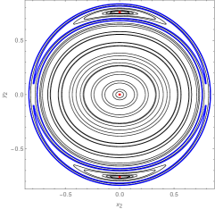
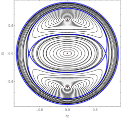
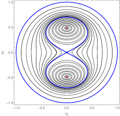
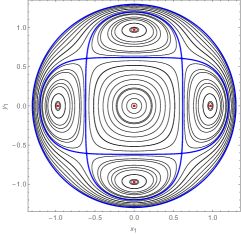
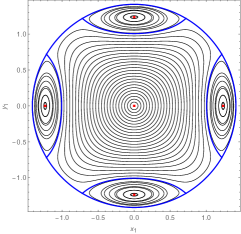
Figure 7: Sequence of $x_{2},y_{2}$ surfaces of section (above) and corresponding $x_{1},y_{1}$ surfaces of section (below) in Case III.

In Fig. 7, a typical sequence of surfaces of section corresponding to Case III is shown to give an impression on how the abstract Fig. 6 translates to the concrete dynamics. The surfaces of section of the other cases are different, but the way how they relate to the corresponding part of Fig. 6 is similar.

5 Bifurcations in the original system

If a normalization is carried far enough to obtain only isolated equilibria (after symmetry reduction), we know the essential characteristics of the system. Including higher orders may shift the positions of the equilibria, but does not alter their number or stability. Therefore the isolated fixed points of (15) correspond to periodic orbits for the original system. The results obtained can be trusted up to low energies, in a neighbourhood of the central equilibrium and not too far from the resonance at hand.

To deduce the periodic orbits of the system from the equilibria of (15), we introduce action angle variables

$$z_{j}\;\;=\;\;\sqrt{2\tau_{j}}\,{\rm e}^{{\rm i}\varphi_{j}}\enspace,\quad j=1,2\enspace.$$ (45)

The singular equilibria correspond to the normal modes of the system. Namely, $\mathcal{Q}_{1}$ corresponds to $\tau_{1}=0$ and $\tau_{2}=\frac{1}{2}\eta$, i.e. to the orbit along the $x_{2}$–axis, in the following also referred to as short axial orbit. Similarly, $\mathcal{Q}_{2}$ gives the orbit along the $x_{1}$–axis, also referred to as long axial orbit, determined by $\tau_{1}=\eta$ and $\tau_{2}=0$.

Remark 5.1

To be consistent with our previous papers, so that the conditions (46) and (47) for banana and anti-banana are the same as in for example [23], one has to exchange sine and cosine in the following.

The regular equilibria correspond to periodic orbits in general position. The equilibrium $\mathcal{U}_{+}$ has co-ordinates $(u,v,w)$ such that $0<u<\eta$, $v<0$ and $w=0$. From (17) we see that it must then be $v=-\sigma_{2}^{2}$ and $\sigma_{1}=0$. By expressing (12) in terms of (45) we get the condition

$$\sigma_{1}\;\;=\;\;\tau_{1}\sqrt{2\tau_{2}}\,\cos(2\varphi_{1}-\varphi_{2})\;\;=\;\;0\enspace,\quad\tau_{1},2\tau_{2}\in\mathopen{]}0,\eta\mathclose{[}\enspace.$$

This implies

$$2\varphi_{1}\;-\;\varphi_{2}\;\;\in\;\;\left\{\frac{\pi}{2},\frac{3\pi}{2}\right\}\enspace.$$ (46)

Similarly, we recognize that the equilibrium $\mathcal{U}_{-}$ corresponds to the condition

$$\sigma_{2}\;\;=\;\;\tau_{1}\sqrt{2\tau_{2}}\,\sin(2\varphi_{1}-\varphi_{2})\;\;=\;\;0\enspace,\quad\tau_{1},2\tau_{2}\in\mathopen{]}0,\eta\mathclose{[}$$

that gives

$$2\varphi_{1}\;-\;\varphi_{2}\;\;\in\;\;\left\{0,\pi\right\}\enspace.$$ (47)

Orbits satisfying (46) and (47) are called, because of their shape in the $(x_{1},x_{2})$–plane, banana orbits and figure-eight or anti-banana orbits, respectively [27]. We found in section 4.1 the critical values (33) and (37) that determine the bifurcations of the reduced system. However, $\eta$ is not a constant for the original system; nevertheless we can use (33) and (37) to find threshold values for the bifurcations in terms of the (generalized) energy $E$. On the long axial orbit ($\tau_{1}=\eta$, $\tau_{2}=0$), the normal form (15) reads as

$$K\;\;=\;\;\eta\;+\;\varepsilon^{2}(2\delta+\alpha_{1}\eta)\eta\;+\;\varepsilon^{4}(\rho_{1}\delta+\alpha_{6}\eta)\eta^{2}\enspace.$$ (48)

Here and in the following, since we refer to the original system, we express the formulas in terms of the coefficients of the original normal form (15). By the scaling of time (9c) we have

$$\frac{\omega_{2}}{2}K\;+\;O(\varepsilon^{6})\;\;=\;\;H\;\;=\;\;E$$ (49)

and combining (48) and (49) we can express the (generalized) energy in terms of $\eta$ as

$$E\;\;=\;\;\frac{\omega_{2}}{2}\left[\eta\,+\,\varepsilon^{2}\left(2\delta+\alpha_{1}\eta\right)\eta\,+\,\varepsilon^{4}(\rho_{1}\delta+\alpha_{6}\eta)\eta^{2}\right]\;+\;O(\varepsilon^{6})\enspace.$$ (50)

Substituting (37) into (50), we find the critical energy threshold values that correspond to the bifurcations off from the long axial orbit, given to second order in $\delta$ by

$$E_{\pm}\;\;:=\;\;-\frac{2\omega_{2}\delta}{4\alpha_{1}-\alpha_{3}}\;+\;\frac{4\omega_{2}\delta^{2}}{(4\alpha_{1}-\alpha_{3})^{3}}\,\left[(4\alpha_{1}-\alpha_{3})(2\beta_{1}+\beta_{2}-2\alpha_{1}+\alpha_{3})\,-\,2(\gamma\pm\mu)\right]$$ (51)

for banana (upper signs) and anti-banana (lower signs) orbits, respectively. Recall $\beta_{1}=\rho_{1}+\frac{1}{4}\rho_{2}-\frac{1}{2}\rho_{3}$ and $\beta_{2}=\frac{1}{2}\rho_{3}-\frac{1}{2}\rho_{2}$ from (20a) and from (37) that $\gamma=6\gamma_{1}+4\gamma_{2}+2\gamma_{3}=6\alpha_{6}-\alpha_{4}$. We inverted the detuning scaling (9b), so that (51) and (52) are expressed in terms of the original detuning parameter. Similarly, for the bifurcation off from the short axial orbit ($\tau_{1}=0$, $\tau_{2}=\frac{1}{2}\eta$) we use (33) and find to second order in $\delta$ that

$$E_{1}\;\;=\;\;-\frac{2\omega_{2}\delta}{\alpha_{3}-\alpha_{2}}\;+\;\frac{2\omega_{2}\delta^{2}}{(\alpha_{3}-\alpha_{2})^{3}}\,\left[(\alpha_{3}-\alpha_{2})(2\beta_{2}+\alpha_{2})\,-\,8\gamma_{3}\right]$$ (52)

where $\beta_{2}=\frac{1}{2}\rho_{3}-\frac{1}{2}\rho_{2}$ and $\gamma_{3}=\frac{1}{4}\alpha_{5}-\frac{3}{8}\alpha_{7}$. However, above a certain threshold one should not expect that the formal series developed by the normalization procedure stays close for a very long time to the solutions of the original problem. Since we pushed the normalization up to including terms of $6$th order in the phase space variables $(x,y)$, we can trust such quantitative predictions on the bifurcation and stability of the periodic orbits up to the second order in the detuning parameter (since, we recall, this is assumed to be a second order term). We can summarize these results as follows.

Theorem 5.2

Let us consider the dynamical systems defined by $H$, cf. (2) and its normal form (15) with respect to the oscillator symmetry (11). Assume the co-ordinate system to be rotated so that $\mu>0$ and $\nu=0$ in (15). In a neighbourhood of the central equilibrium and for sufficiently small values of the detuning parameter $\delta$,

• at the stability/instability transition of a normal mode, periodic orbits in general position bifurcate. In particular, at each transition of the long axial orbit, a pair of periodic orbits bifurcate (a pair of banana or a pair of anti-banana orbits). At the instability of the short axial orbit, two pairs of periodic orbits (a pair of banana and a pair of anti-banana orbits) bifurcate concurrently;

• up to second order in the detuning, the instability/stability transition of the normal modes occur at the critical energies (51) and (52) for the long and short normal mode, respectively.

The coefficients $\alpha$ and $\lambda$ determine the possible bifurcation sequences according to the previous section. Recalling that $2(\alpha+2\lambda)=4\alpha_{1}-\alpha_{3}$ and $2\alpha=\alpha_{3}-\alpha_{2}$, the analysis that resulted into Cases I–V can be rewritten in terms of the periodic orbits of the original system.

Theorem 5.3

Under the conditions of theorem 5.2 the possible bifurcation sequences are determined by the coefficients $\alpha_{1}$, $\alpha_{2}$, $\alpha_{3}$ in the normal form (15). For $\alpha_{3}\neq\alpha_{2}$, $\alpha_{3}\neq 2\alpha_{1}+\frac{1}{2}\alpha_{2}$, $\alpha_{3}\neq 4\alpha_{1}$ and $\delta<0$ we have the following cases.

Case I. $\alpha_{3}-\alpha_{2}<0<4\alpha_{1}-\alpha_{3}$. The short axial orbit is always stable. The long axial orbit changes its stability twice. At first it suffers a transition to instability at the critical energy $E=E_{+}$ and a pair of stable banana orbits appears. At $E=E_{-}$ a pair of anti-banana orbits appears, while the long axial orbit comes back to stability.

Case II. $0<\alpha_{3}-\alpha_{2}<4\alpha_{1}-\alpha_{3}$. While the (generalized) energy passes through the critical values $E=E_{+}$ and subsequently $E=E_{-}$, the bifurcation sequence follows the previous case. However a further bifurcation occurs at $E=E_{1}$, when both pairs of periodic orbits in general position disappear on the short axial orbit.

Case III. $0<4\alpha_{1}-\alpha_{3}<\alpha_{3}-\alpha_{2}$. At $E=E_{1}$ a pair of banana and a pair of anti-banana orbits bifurcate off from the short axial orbit. The banana orbits are unstable and the anti-banana orbits are stable. At $E=E_{+}$ banana orbits disappear on the long axial orbits, which becomes unstable. At $E=E_{-}$ anti-banana orbits disappear as well, and the long axial orbit turns back to stability.

Case IV. $4\alpha_{1}-\alpha_{3}<0<\alpha_{3}-\alpha_{2}$. At $E=E_{1}$ a bifurcation occurs from the short axial orbit, and the two pairs of periodic orbits in general position appear. Banana orbits are unstable and anti-banana orbits are stable. The long axial orbit is always stable.

Case V: $4\alpha_{1}<\alpha_{3}<\alpha_{2}$. The only periodic orbits are the normal modes, both stable.

The undetuned system for $\delta=0$ behaves as in Cases I or IV (after the bifurcations) if $\alpha_{3}-\alpha_{2}$ and $4\alpha_{1}-\alpha_{3}$ have opposite signs and otherwise as in Case V.

Assuming the co-ordinate system to be such that $\nu$ vanishes in the normal form (15) is not needed for qualitative predictions, but only for quantitative ones. And even here the necessary rotation can simply be turned back. In fact, the presence of $\nu$ would not change the possible bifurcation scenario of the system, but would affect the value of the energy thresholds (51) and (52) — replacing $\mu$ by $\sqrt{\mu^{2}+\nu^{2}}$.

Remark 5.4

Let us note one more time that for definiteness we assumed $\mu$ positive and $\delta$ negative. Taking $\delta>0$ yields the red cases I–V; as a demonstration see the example in section 6. Since the difference in the bifurcation thresholds (51) is proportional to $\mu(4\alpha_{1}-\alpha_{3})^{-3}$, a change in the sign of $\mu$ would affect only the bifurcation order of banana and anti-banana orbits, that consequently would also exchange their stability properties, as would a change in the sign of $4\alpha_{1}-\alpha_{3}$.

6 Galactic dynamics under power law potentials

To demonstrate our results with an example, let us consider the family of potentials

$$V(x_{1},x_{2};q,p)\;\;=\;\;\frac{1}{p}\left(1+x_{1}^{2}+\frac{x_{2}^{2}}{q^{2}}\right)^{p/2}\enspace,\quad\mbox{$0<p<2$, $\frac{1}{4}<q\leq 1$}.$$ (53)

This gravitational potential is generated by a simple but realistic matter distribution [32, 28, 34, 33, 3]. Its astrophysical relevance [4, 5] is based on the ability to describe in a simple way the gross features of elliptical galaxies embedded in a dark matter halo. Here the lower limit $p\to 0$ corresponds to the logarithmic potential, while the upper limit $p\to 2$ is dictated by the assumption of a potential generated by a positive mass distribution.

The flattening is $1/q$ and we slightly extend its range from the range $\frac{1}{2}<q\leq 1$ used in [23] that is typically associated with elliptical galaxies [27] as it is precisely at $q=\frac{1}{2}$ that the $2{:}4$ resonance occurs. Lower positive values of $q$ can in principle be considered but correspond to an unphysical density distribution. The truncated series expansion (2) is “prepared” for normalization by setting

$$q\;\;=\;\;\frac{\omega_{1}}{\omega_{2}}\;\;=\;\;\frac{1}{2}\;+\;\delta\enspace,$$ (54)

the canonical variables and time are rescaled according to (9) and we expanded in series of the detuning according to (54). The coefficients of the normal form (15) read as

$$\alpha_{1}=\frac{3}{2}B_{1},\;\;\alpha_{2}=6B_{1},\;\;\alpha_{3}=4B_{1},\;\;\rho_{1}=3B_{1},\;\;\rho_{2}=-12B_{1},\;\;\rho_{3}=0$$ (55a)

$$\alpha_{4}=-\frac{56}{3}B_{1}^{2}+9B_{2},\;\;\alpha_{5}=-\frac{2}{3}(46B_{1}^{2}-27B_{2}),\;\;$$ (55b)

$$\alpha_{6}=\frac{17B_{1}^{2}-10B_{2}}{4},\;\;\alpha_{7}=-2(17B_{1}^{2}-10B_{2}),\;\;$$ (55c)

$$\mu\;=\;3(2B_{1}^{2}-B_{2}),\quad\nu\;=\;0\enspace,$$ (55d)

where

$$B_{1}\;=\;\frac{p-2}{8}\quad\mbox{and}\quad B_{2}\;=\;\frac{(p-2)(p-4)}{48}\enspace,$$ (56)

compare with [23]. As the potential is scalar, the ensuing system is reversible with respect to

$$(x_{1},x_{2})\;\;\mapsto\;\;(x_{1},-x_{2})$$ (57)

which through reduction turns into

$$(u,v,w)\;\;\mapsto\;\;(u,v,-w)$$

and explains why $\nu=0$. By substituting (55) into (20) we find

$$\lambda\;=\;-\alpha\;=\;\frac{p-2}{8}\;<\;0\quad\mbox{and}\quad\mu\;=\;\frac{1}{32}(p^{2}-4)\;<\;0\enspace.$$ (58)

Note that the $\pi$–rotation $(u,v,w)\mapsto(u,-v,-w)$ still allows to achieve $\mu>0$ in (58), if necessary. According to theorem 5.3 and remark 5.4, the coefficients $\alpha_{j}$, $j=1,2,3$ determine the bifurcation sequences. Since $4\alpha_{1}-\alpha_{3}<0<\alpha_{3}-\alpha_{2}$ and, concentrating on $q>\frac{1}{2}$, the detuning $\delta$ is positive, the bifurcation sequence follows Case I of theorem 5.3 (in which remember to reverse all the inequalities, according to remark 5.4). As $\mu$ is negative, bifurcations occur always from the long normal mode, with bananas appearing at lower energies than anti-bananas. The critical values of the energy that determine the bifurcations can be found by substituing (55d) and (56) into (51) and, expressed in terms of the parameters of (53), in agreement with [23] read as

$$E_{+} \;\;=\;\;\frac{16}{2-p}\left(q-\frac{1}{2}\right)\;+\;\frac{8(41p-10)}{3(p-2)^{2}}\left(q-\frac{1}{2}\right)^{2}$$ (59a)

$$E_{-} \;\;=\;\;\frac{16}{2-p}\left(q-\frac{1}{2}\right)\;+\;\frac{8(53p+14)}{3(p-2)^{2}}\left(q-\frac{1}{2}\right)^{2}$$ (59b)

for the bifurcation of banana and anti-banana orbits, respectively. Numerical values of the thresholds when applied e.g. to the logarithmic potential (taking $p=0$), are in good agreement with the bifurcation values obtained from numerical computations [27].

Remark 6.1

When modeling the dynamics in a rotating galaxy using the Hamiltonian function

$$H(x,y)\;\;=\;\;\frac{y_{1}^{2}+y_{2}^{2}}{2}\;-\;\Omega(x_{1}y_{2}-x_{2}y_{1})\;+\;V(x_{1},x_{2};q,p)\enspace,$$ (60)

we generalize (53) which is the limit of (60) as $\Omega\to 0$. Due to the rotation of the galaxy, the Hamiltonian (60) does not respect the symmetries (1). However, after diagonalization of the quadratic part, its series expansion still has the form (2). With the assumption that the angular velocity $\Omega$ is a small parameter and $\frac{1}{4}<q\leq 1$ as above, the system can again be studied as a perturbation of an oscillator close to a $1{:}2$ resonance. Since all the terms not respecting the symmetries (1) do not Poisson commute with the $1{:}2$ oscillator and odd order terms are not present in the series expansion of (60), a normalization of the (truncated) diagonalized Hamiltonian then results in the normal form of a $2{:}4$ (detuned) resonance, thus still of the form (15). Compared with (53), the presence of quartic terms of odd order in the momenta in the diagonalized Hamiltonian produces non-vanishing $\nu$. Modulo a rotation to eliminate $\nu$, theorems 5.2 and 5.3 can be applied. The resulting families of periodic orbits would however correspond to more “fancy” orbits for the original system (60), once the diagonalizing transformation is inverted. We leave a deeper analysis of this problem to future work.

Several results of the theory developed above can be extended to a $3$–dimensional model of the form

$$H(x,y)\;\;=\;\;\frac{y_{1}^{2}+y_{2}^{2}+y_{3}^{2}}{2}\;+\;V(x_{1},x_{2},x_{3})\enspace,$$ (61)

in the cases in which the mirror symmetries (1) are extended to the third axis when composing with the transformation law

$$(x_{3},y_{3})\;\;\mapsto\;\;(-x_{3},-y_{3})\enspace.$$ (62)

Each symmetry plane of the potential generates an invariant subset where the dynamics essentially reduce to those investigated above. By introducing a further detuning parameter associated to the second frequency ratio, bifurcation and stability of periodic orbit families on the symmetry planes can be deduced. The validity of this approach is supported by analogous results obtained with the $1{:}1{:}1$ resonance [37, 12, 15]. For a deeper understanding, $3$–dimensional normal forms of the symmetric $1{:}1{:}2$, $1{:}2{:}2$ and $1{:}2{:}4$ resonances are necessary [1, 2, 31], which usually provide the properties of periodic orbits in general position. Note that a normal form of the $1{:}2{:}2$ resonance is always integrable, while already the cubic normal forms of the $1{:}1{:}2$ and $1{:}2{:}4$ resonances are not integrable [8]. However, the discrete symmetries not only make the cubic terms vanish but may furthermore enforce some of the non-trivial normal forms to be integrable, see [17].

7 Conclusions

We considered families of Hamiltonian systems in two degrees of freedom with an equilibrium in $2{:}4$ resonance, a $1{:}2$ resonance with additional discrete symmetry. Under detuning, this typically leads to normal modes losing their stability through period-doubling bifurcations. This now concerns the long axial orbit, losing and regaining stability through two period-doubling bifurcations. In galactic dynamics one speaks of banana and anti-banana orbits. The short axial orbit turns out to be dynamically stable everywhere except at a simultaneous bifurcation of banana and anti-banana orbits.

We excluded the case $\mu=0$ from our considerations since it would require further normalization. Indeed, for $\mu=0$ the normal form (15) resembles (22) and leads to a similar degeneracy, which to break requires higher order terms that do depend on $v$ (or on $w$). One may speculate that for such a $k{:}2k$ resonance, $k\geq 3$ also the conical singularity $\mathcal{Q}_{2}$ “turns into” a cusp and the two successive period-doubling bifurcations of the long periodic orbit occur simultaneously, as it happens to the two successive period-doubling bifurcations of the short periodic orbit when the $1{:}2$ resonance becomes the $2{:}4$ resonance.

References

- [1] E. van der Aa, First-order resonances in three-degrees-of-freedom systems, Cel. Mech., 31, 163–191 (1983)
- [2] E. van der Aa and F. Verhulst, Asymptotic Integrability and Periodic Solutions of a Hamiltonian System in –Resonance, SIAM, 15, 890–911 (1984)
- [3] C. Belmonte, D. Boccaletti and G. Pucacco, On the orbit structure of the logarithmic potential, Ap. J., 669, 202–217 (2007)
- [4] J. Binney, Resonant excitation of motion perpendicular to galactic planes, MNRAS, 196, 455–467 (1981)
- [5] J. Binney and S. Tremaine, Galactic Dynamics. Princeton University Press (2008)
- [6] D. Boccaletti and G. Pucacco, Theory of Orbits, Vol. 2, Chapter 8. Springer (1999)
- [7] H. W. Broer, I. Hoveijn, G. A. Lunter and G. Vegter, Resonances in a spring-pendulum: algorithms for equivariant singularity theory, Nonlinearity, 11, 1569–1605 (1998)
- [8] O. Christov, Non-integrability of first order resonances of Hamiltonian systems in three degrees of freedom, Cel. Mech. Dyn. Astr., 112, 147–167 (2012)
- [9] G. Contopoulos, Order and Chaos in Dynamical Astronomy. Springer (2004)
- [10] R. H. Cushman and L. M. Bates, Global aspects of classical integrable systems. Birkhäuser (1997)
- [11] R. H. Cushman, H.R. Dullin, H. Hanßmann and S. Schmidt, The resonance, Regular and Chaotic Dynamics, 12, 642–663 (2007)
- [12] R. H. Cushman, S. Ferrer and H. Hanßmann, Singular reduction of axially symmetric perturbations of the isotropic harmonic oscillator, Nonlinearity, 12, 389–410 (1999)
- [13] K. Efstathiou, Metamorphoses of Hamiltonian systems with symmetries. Lecture Notes in Mathematics 1864, Springer (2005)
- [14] K. Efstathiou, H. Hanßmann and A. Marchesiello, Bifurcations and Monodromy of the Axially Symmetric Resonance, Journal of Geometry and Physics 146, 103493, 1–30 (2019)
- [15] S. Ferrer, J. Palacián and P. Yanguas, Hamiltonian Oscillators in Resonance: Normalization and Integrability, Journal of Nonlinear Science 10, 145–174 (2000)
- [16] H. Hanßmann, Local and Semi-Local Bifurcations in Hamiltonian Dynamical Systems — Results and Examples. Lecture Notes in Mathematics 1893, Springer (2007)
- [17] H. Hanßmann, R. Mazrooei-Sebdani, F. Verhulst, The resonance in a particle chain, preprint, ArXiv 2002.01263 (2020)
- [18] H. Hanßmann and J.C. van der Meer, On the Hamiltonian Hopf bifurcations in the Hénon–Heiles family, J. Dynamics Diff. Eq., 14, 675–695 (2002)
- [19] H. Hanßmann and B. Sommer, A degenerate bifurcation in the Hénon–Heiles Family, Cel. Mech. Dyn. Astr., 81, 249–261 (2001)
- [20] M. Iñarrea, V. Lanchares, J. Palacián, A.I. Pascual, J.P. Salas and P. Yanguas, Reduction of some perturbed Keplerian problems, Chaos, Solitons and Fractals, 27, 527–536 (2006)
- [21] V. V. Kozlov, Symmetries, Topology and Resonances in Hamiltonian Mechanics. Springer (1991)
- [22] A. Marchesiello and G. Pucacco, The symmetric resonance, Eur. Phys. J. Plus, 128, 21, 1–14 (2013)
- [23] A. Marchesiello and G. Pucacco, Resonances and bifurcations in systems with elliptical equipotentials, MNRAS, 428, 2029–2038 (2013)
- [24] A. Marchesiello and G. Pucacco, Equivariant singularity analysis of the resonance, Nonlinearity, 27, 43–66 (2014)
- [25] J. C. van der Meer, The Hamiltonian Hopf bifurcation. Lecture Notes in Mathematics 1160, Springer (1985)
- [26] K. R. Meyer, J. F. Palacián and P. Yanguas, Singular reduction of resonant Hamiltonians, Nonlinearity, 31, 2854–2894 (2018)
- [27] J. Miralda-Escudé and M. Schwarzschild, On the orbit structure of the logarithmic potential, Ap. J., 339, 752–762 (1989)
- [28] Y. Papaphilippou and J. Laskar, Frequency map analysis and global dynamics in a two degrees of freedom galactic potential, Astron. Astrophys., 307, 427–449 (1996)
- [29] G. Pucacco and A. Marchesiello, An energy-momentum map for the time-reversal symmetric resonance with symmetry, Physica D, 271, 10–18 (2014)
- [30] J. A. Sanders, Are higher order resonances really interesting?, Cel. Mech., 16, 421–440 (1978)
- [31] J. A. Sanders, F. Verhulst and J. Murdock, Averaging Methods in Nonlinear Dynamical Systems, Second Edition. Appl. Math. Sciences 59, Springer (2007)
- [32] P. Scuflaire, Stability of axial orbits in analytical galactic potentials, Cel. Mech. Dyn. Astr., 61, 261–285 (1995)
- [33] P. Scuflaire, Periodic orbits in analytical planar galactic potentials, Cel. Mech. Dyn. Astr., 71, 203–228 (1999)
- [34] J. Touma and S. Tremaine, A map for eccentric orbits in non-axisymmetric potentials, MNRAS, 292, 905–919 (1997)
- [35] J. M. Tuwankotta and F. Verhulst, Symmetry and Resonance in Hamiltonian Systems, SIAM J. Appl. Math., 61, 1369–1385 (2000)
- [36] F. Verhulst, Discrete-symmetric dynamical systems at the main resonances with applications to axi-symmetric galaxies, Phil. Trans. Royal Soc. London A, 290, 435–465 (1979)
- [37] T. de Zeeuw, Motion in the core of a triaxial potential, MNRAS, 215, 731–760 (1985)
- [38] T. de Zeeuw and D. Merritt, Stellar orbits in a triaxial galaxy. I. Orbits in the plane of rotation, Ap. J., 267, 571–595 (1983)