Markov Chains for Horizons (MARCH). I. Identifying Biases in Fitting Theoretical Models to Event Horizon Telescope Observations
Abstract
We introduce a new Markov Chain Monte Carlo (MCMC) algorithm with parallel tempering for fitting theoretical models of horizon-scale images of black holes to the interferometric data from the Event Horizon Telescope (EHT). The algorithm implements forms of the noise distribution in the data that are accurate for all signal-to-noise ratios. In addition to being trivially parallelizable, the algorithm is optimized for high performance, achieving 1 million MCMC chain steps in under 20 seconds on a single processor. We use synthetic data for the 2017 EHT coverage of M87 that are generated based on analytic as well as General Relativistic Magnetohydrodynamic (GRMHD) model images to explore several potential sources of biases in fitting models to sparse interferometric data. We demonstrate that a very small number of data points that lie near salient features of the interferometric data exert disproportionate influence on the inferred model parameters. We also show that the preferred orientations of the EHT baselines introduce significant biases in the inference of the orientation of the model images. Finally, we discuss strategies that help identify the presence and severity of such biases in realistic applications.
1 INTRODUCTION
Images of low-luminosity black holes at millimeter wavelengths, where the accretion flow is transparent down to horizon scales (Özel et al., 2000), have long been expected to be compact, dominated by the shadow cast by the black hole on the surrounding plasma emission (Falcke et al., 2000; Dexter et al., 2009; Broderick et al., 2009; Mościbrodzka et al., 2009, 2014; Chan et al., 2015). Recent Event Horizon Telescope (EHT) observations of the black hole in the center of the M87 galaxy have confirmed this expectation, revealing an image consisting of a narrow ring of emission surrounding the black-hole shadow (Event Horizon Telescope Collaboration et al., 2019a, b, c, d, e, f).
As a Very Long Baseline Interferometric (VLBI) array, the EHT measures the complex Fourier components of the brightness distribution in the sky, also called the interferometric visibilities, at a distinct set of spatial frequencies determined by the baselines between the various stations in the array. In principle, the image of the source can then be obtained by constructing the inverse Fourier transform of the observed visibilities. In practice, however, the sparse coverage of Fourier space by the EHT, which consists of a small number of baselines separated by large distances, makes such a direct reconstruction of the image impossible.
Traditionally, VLBI measurements have been converted to images with CLEAN algorithms (see, e.g., Högbom 1974; Clark 1980), which identify the minimum set of point sources in the image plane with Fourier transforms that are consistent with the visibility data. These point sources are then convolved with a filter to broaden the points sources to the effective resolution of the interferometric array.
Alternatively, interferometric images have been obtained with regularized maximum likelihood methods in which a pixel-based model is defined in the image plane with its parameters being the brightness at each pixel location. The Fourier transform of this model is compared to the observed visibilities and the brightness of each pixel is adjusted to minimize an appropriate -statistic in visibility space. Because the number of pixels of the model image is typically much larger than the number of measurements, regularizers are employed to decrease the effective number of degrees of freedom. This approach was introduced in radio interferometry imaging with maximum-entropy regularizers (see Narayan & Nityananda 1986 and references therein), has been developed extensively in optical/IR interferometry (Thiébaut, 2009; Berger et al., 2012), and has been employed in imaging black holes with the EHT (see, e.g., Honma et al. 2014; Chael et al. 2016, 2018; Akiyama et al. 2017b, a; Event Horizon Telescope Collaboration et al. 2019d).
The regularized maximum likelihood methods are fundamentally non-parametric model fitting algorithms. As such, they are agnostic in regards to the underlying image structure. However, this freedom comes with the usual “curse of dimensionality”: the requirement of quantifying the brightness on a very large number of pixels typically leads to presenting a single (or a very small number of) best-fit images with marginal exploration of the parameter space of possible solutions that might fit the data equally well. Moreover, the image properties show a dependence on the regularizers and the strength of the regularizers is usually chosen such that they suppress structures at scales smaller than the effective beam of the array (see, e.g., Event Horizon Telescope Collaboration et al. 2019d). This limits the ability of the algorithms to provide precise measurements of physical quantities of interest.
In order to elucidate the limitations of an agnostic imaging algorithm, we can consider interferometric observations of a simple source consisting of two point sources separated by some angular distance. An imaging algorithm will only be able to measure the separation of the two point sources down to an accuracy comparable to the effective beam size of the array, which depends mainly on the wavelength of observation and the separations of the interferometric stations. However, if we know a priori that we are looking at an image with two point sources, we can use the same interferometric data to measure the angular separation of the point source with a much higher accuracy that will be limited primarily by the signal-to-noise ratio of the measurements. Achieving such a measurement for a realistic image, of course, requires both an accurate parametric model for the underlying image as well as an algorithm to explore the posterior distribution of the statistical comparison of the model to the data.
In the first article of this series, we describe the new Markov-Chain Bayesian algorithm MARCH (MArkov Chains for Horizons) that we have developed to fit models of black-hole images to the interferometric data at mm wavelengths obtained with the EHT. Similar Bayesian approaches have already been applied to early EHT observations of the galactic center black hole Sgr A* (see, e.g., Broderick et al. 2016; Lu et al. 2018) as well as to the 2017 EHT observations of M87 that have led to the initial measurements of the mass of the latter black hole (Event Horizon Telescope Collaboration et al., 2019f). Our algorithm aims to address a number of complications to this otherwise straightforward statistical problem introduced by theoretical expectations on the images of black holes and the particular characteristics of the EHT array.
First, the structure of the mm image of Sgr A* is expected to show substantial variability within the few-hour time span of the observations because of its small mass (see, e.g., Medeiros et al. 2017, 2018; Roelofs et al. 2017). As a result, fitting a static model image to variable interferometric data will introduce biases to the inferred parameters and artificially reduce their inferred uncertainties. This complication was addressed in earlier work (Kim et al., 2016) and we will not revisit it here.
Second, the images of black holes with horizon-scale resolution are expected to have ring-like structures with very sharp boundaries at the locations of the black-hole shadows (see, e.g., Kamruddin & Dexter 2013; Psaltis et al. 2015). The interferometric visibilities of these structures show a number of salient features such as deep minima of the visibility amplitudes at particular baseline lengths, with rapid swings of the visibility phases across them. The location of the first minimum depends very strongly on the size of the ring of emission and the location of the second minimum depends on its fractional width (Event Horizon Telescope Collaboration et al., 2019f). While the strong dependence of the salient features on model parameters allows us to measure them accurately, the most likely values of the model parameters and their uncertainties depend disproportionately on how well the model describes the very small number of data points near the salient features. As we will show in §3, the combination of the simplicity of the model images with the high signal-to-noise ratio of the measurements causes a straightforward application of Bayesian posteriors to return biased measurements of the model parameters.
Finally, the location of landmass and high mountains on the globe forces the EHT baselines to lie primarily along two orientations, N-S and E-W (Event Horizon Telescope Collaboration et al., 2019b). As a result of the projection-slice theorem, the measured interferometric visibilities are primarily sensitive only to the projections of the underlying image along these two orientations. We will show in §4 that this biases the inferred orientations of the model images to line up with the major orientations of the baselines. The origin of this bias is similar to the development of spurious “knots” along the baseline orientations in the reconstruction of otherwise smooth images from synthetic EHT data (see Fig.10 of Event Horizon Telescope Collaboration et al. 2019d). Additional evidence for this effect comes from the initial application of geometric and GRMHD model fitting to the 2017 EHT data of M87, which revealed that the most likely black-hole orientation appears aligned with the orientations of the EHT baselines (see Fig. 6 of Event Horizon Telescope Collaboration et al. 2019f) and away from the orientation of the long-wavelength jet that emerges from the central black hole (see Fig. 9 of Event Horizon Telescope Collaboration et al. 2019e).
In §2 below, we introduce the basic formalism of our Bayesian Markov Chain algorithm and its implementation. In §3-5, we apply this algorithm to various cases of simple synthetic data chosen to explore the issues discussed above and provide strategies for their mitigation. In §6, we explore realistic EHT data based on GRMHD simulations of M87 and, in §7, we conclude by discussing our results and providing an outlook on the accuracy of measurements with the EHT. In subsequent papers in this series, we will discuss our implementation of modeling the unknown gains of the various interferometric stations and the biases introduced by this approach; we will also explore different information criteria that allow us to quantify the necessity of increasing the complexity of models in order to fit realistic data.
2 The MARCH Algorithm
2.1 Interferometric Observables
The goal of the MARCH algorithm is to estimate the posterior distributions over a number of parameters of a model by comparing to EHT observations the model image brightness in the sky ; here and are angular coordinates and is the vector of model parameters. As an interferometer, the EHT does not directly observe the brightness distribution of the sky but rather the complex visibilities defined by the van Cittert-Zernike theorem as
| (1) |
In this equation, and are equal to the two components of the baseline vectors that connect every pair of sites in the array, projected orthogonally to the line of sight to a particular source, and divided by the wavelength of observation, i.e., . The brightness distribution in the image domain and the visibilities in the domain are clearly connected via a 2-dimensional Fourier transform.
For a general, non symmetric brightness distribution, the interferometric visibilities are complex numbers that can be described either in terms of their real and imaginary components or in terms of their amplitudes and phases. The former description is useful in quantifying the thermal noise in the measurements, which can be well approximated by independent Gaussian distributions in the real and imaginary components of the visibilities (see Thompson et al. 2017). However, because of atmospheric and instrumental effects, seldom do VLBI measurements allow for a precise determination of the complex visibilities. In practice, we write the measured visibility between the th and station as
| (2) |
where and are complex “gains” of the two telescopes and a star superscript denotes complex conjugates. Hereafter, as in this equation, we will denote the visibilities between the two stations simply as and suppress for brevity the argument of this quantity.
The magnitudes of the gain factors for the various telescopes can often be constrained with a priori calibration to within % levels (Event Horizon Telescope Collaboration et al., 2019c). On the other hand, the complex phases of the gains can fluctuate wildly and over very short timescales because of atmospheric instabilities and instrumental effects. To overcome this problem, VLBI measurements quote the amplitudes of the complex visibilities between pairs of stations and the arguments of the complex bispectra (also known as closure phases) along a closed triangle of stations (Jennison, 1958; Thompson et al., 2017). The latter is simply
| (3) | |||||
i.e., the closure phases are not affected by the unknown phases of the telescope gains.
We pay three penalties by using visibility amplitudes and closure phases instead of the real and imaginary components of the complex interferometric visibilities. First, by combining three complex visibilities to form one closure quantity, we lose some of the available information. Second, the transformation between the brightness in the image domain and the observables in the visibility domain is no longer linear. As a result, adding a perturbation to an image that would only introduce minor variations in the complex visibilities could still lead to order unity changes in visibility amplitudes and closure phases at various baseline lengths. This is important in understanding the consequences of the strong dependence of model parameters on the salient features of the visibilities. Third, the error distributions of the visibility amplitudes and closure phases are not Gaussian, even for purely thermal noise.
The likelihood of making a visibility amplitude measurement given a true visibility amplitude of is the Rice distribution (Thompson et al., 2017)
| (4) |
where is the modified Bessel function of zeroth order and is the dispersion of thermal noise introduced to the real and imaginary components of the visibility by the array configuration used. At large signal-to-noise ratios , the Rice distribution reduces to a Gaussian with the same dispersion. The computational cost of using the Rice distribution is only marginally higher than using the Gaussian approximation.
The likelihood of making a closure phase measurement is given by the triple convolution
| (5) |
Here is the true closure phase and is the likelihood of measuring for the phase of the baseline an angle away from the true value. This last likelihood is given by (Thompson et al., 2017)
| (6) | |||||
where is the signal-to-noise ratio of the measurement. The triple convolution necessary to calculate the likelihood for the closure phase is too expensive computationally. Christian & Psaltis (2019) developed an efficient numerical algorithm that allows us to obtain an accurate approximation to the complete likelihood (5), which we use here. At the limit of large signal-to-noise ratios, this distribution can be well approximated by a Gaussian with dispersion
| (7) |
2.2 Bayesian Posteriors
Given a set of interferometric data points, we calculate the posterior distribution of the model parameters using Bayes’ theorem, i.e.,
| (8) |
Here, is the prior distribution over the model parameters, is the likelihood that the set of observed data can be obtained from a given set of model parameters, and is a normalization constant.
The likelihood function is obtained by a proper combination of the likelihoods of the visibility amplitude and closure phase data, equations (4) and (5), respectively. Writing schematically the likelihood of the th data point as and assuming that all likelihoods are independent of each other (see Blackburn et al. 2019), we obtain
| (9) |
The priors over the model parameters depend on the specifics of the model considered. For the analytic crescent model we will be using below, we set all the priors to boxcar functions with limits that are much larger than the widths of the expected posteriors. For reasons that will be discussed in the following sections, the posteriors have very small fractional widths (often less than 1%) and, therefore, the precise function form of such non-informative priors does not affect the final results.
2.3 Markov Chains, Parallel Tempering, and Performance
The sparse coverage of the plane with the EHT baselines results in a small number of independent measurements and hence warrants fitting models to the data that only have a relatively small number of parameters. Moreover, the salient features of the interferometric data, such as the baseline lengths that correspond to minima in the visibility amplitude, allow for relatively accurate initial guesses for the values of several model parameters (see the discussion in §3 and §4 below). For these reasons, we employ a simple Metropolis-Hastings stepping algorithm for each chain of the MCMC algorithm. In particular, we choose steps for each model parameters from independent Gaussian distributions with dispersions set equal to a fraction of the expected uncertainties in the corresponding model parameters.
The presence of salient features in the interferometric data often leads to narrow widths for the posteriors and strong correlations between some model parameters (see §4 below). In order to both efficiently explore the broad parameter space and take small steps to sample the narrow posteriors, we employ a parallel tempering strategy, as discussed, e.g., in Earl & Deem (2005). In this approach, the posteriors are sampled at various levels, i.e., replicas, each of which has been artificially broadened by some a priori chosen temperature. Each successive replica in the ladder has an increasing temperature, i.e., corresponding to a larger broadening. Only the lowest level replica, which corresponds to no broadening, is used for the final calculation of the posteriors. However, the other replicas help sample the parameter space more efficiently and increase the chance that a Markov-Chain step will get closer to and sample a region of high posterior. The number and spacing of the parallel tempered ladders (the replicas) we use depends on the complexity of the data and of the model. For the examples with the synthetic data we use in this paper, we typically use a ladder of 40 replicas with temperatures increasing from the lowest replica in multiples of from unity.
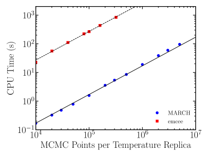
Like all MCMC algorithms, MARCH is trivially parallelizable. However, special care was given in its development to boost its computational efficiency and performance in order to enable fitting complex, numerical models to the interferometric data. In particular, we ensured that computationally expensive operations (such as logs, powers, and trigonometric functions) are only sparsely used and organized the algorithmic flow in such a way that the same quantity is not repeatedly computed. As a result, for analytic models, MARCH achieves very high performance even on a single CPU.
Figure 1 shows the CPU time (on a Macbook Air with an 1.6 GHz Intel Core i5 processor) per temperature replica as a function of MCMC chain steps, for the synthetic data problem discussed in §3 below. In this example, 152 data points were fit with an analytic crescent model described by 5 model parameters, with the MCMC stepping per parameter adjusted such that the average acceptance ratio of the zero-temperature chain is equal to 20%. The figure demonstrates the linear scaling of the algorithm on the number of MCMC chain steps and its high performance, which reaches (for this example) seconds per MCMC steps. The figure also compares the performance of MARCH to that of a commonly used Python MCMC algorithm (emcee; Foreman-Mackey et al. 2013), running the identical problem. The fact that MARCH was optimized for the problem under consideration leads to an increase in performance by a factor of compared to the more general emcee algorithm.
3 An Analytic Model of Crescent Images
In order to explore some of the characteristics of fitting models to the EHT visibility data, we will employ here the geometric model of a crescent image devised by Kamruddin & Dexter (2013). This model creates a crescent by subtracting the brightness of two uniform but displaced disks. Additional complexities to the model were added in Benkevitch et al. (2016), who allowed for a gradient in the brightness across the crescent, and in Event Horizon Telescope Collaboration et al. (2019f), where a number of displaced Gaussian components were included to the image. Albeit simple, this model captures all the basic characteristics of the images encoded in the first EHT data on M87 (see Event Horizon Telescope Collaboration et al. 2019f).
The complex visibility of a simple crescent image is given by (Kamruddin & Dexter, 2013)
| (10) |
where and are the outer and inner disk angular radii, is the Bessel function of the first kind, is the uniform brightness of the ring, measures the fractional depression of brightness at its center,
| (11) |
is the baseline length in units of the wavelength and the coordinate pair measures the displacement of the center of the inner disk with respect to that of the outer disk along the two orientations in the sky.
In order to simplify our notation, we express the characteristic radius of the crescent in terms of the average radii of the two uniform disks
| (12) |
and the fractional width of the ring as their normalized difference111Note that, in Event Horizon Telescope Collaboration et al. (2019f), the fractional width is defined in terms of the mean diameter, i.e., , such that .
| (13) |
For non-symmetric crescents (i.e., when or ), we define the orientation of the crescent as
| (14) |
and the symmetry of the crescent as
| (15) |
Finally, we normalize the complex visibilities such that they are equal to unity at zero baseline length, i.e., set
| (16) |
Unless otherwise stated, we will set hereafter.
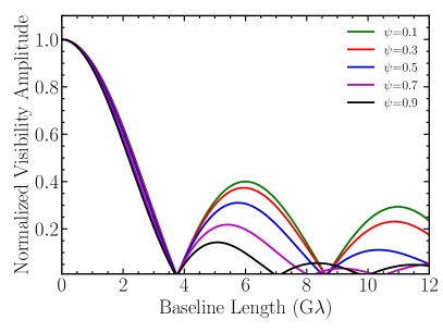
The visibility amplitudes (10) of symmetric rings show the typical ”ringing” of the Bessel functions, with minima at a series of characteristic baseline lengths. For a ring of infinitesimal width, the first minimum occurs at a baseline length of . As the fractional width of the ring increases, the baseline length of the first minimum also increases. This introduces a correlation between the radii and fractional widths of rings that show the first visibility minimum at the same baseline length. An approximate fitting formula for this correlation is (see Event Horizon Telescope Collaboration et al. 2019f)
| (17) |
where is the radius of the infinitesimal ring with the same location of the first visibility minimum. Setting , we get , for rings that show the first visibility minimum at the same baseline length.
Figure 2 shows the normalized visibility amplitudes of symmetric rings with different fractional widths but with radii that follow the correlation given by equation (17). By construction, all these visibility amplitudes have the first visibility minimum at the same baseline length ( G). As the fractional width of the ring increases, the local maximum at G decreases and, for , the location of the second minimum moves towards smaller baseline lengths.
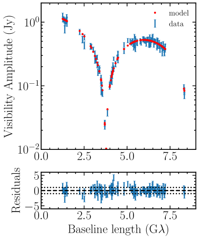
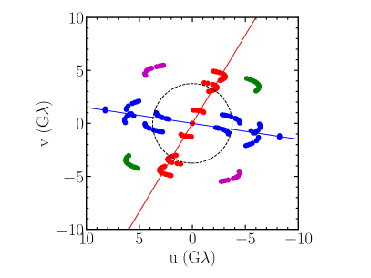
In order to explore the performance of our MCMC algorithm and understand the qualitative aspects of fitting crescent models to EHT data, we generated a set of synthetic visibility amplitude and closure phase data using the crescent model (10) for a symmetric ring () with parameters as, , , , and a flux of Jy. We generated data on the locations of the baselines of the 2017 April 5 EHT observations of M87 (see Fig. 3) and, for the purposes of this exploration, introduced only thermal (Gaussian) errors with standard deviation equal to 10% of the model visibility amplitudes. We then used MARCH to fit the data with the same crescent model. The synthetic visibility amplitudes, the predictions of the best-fit model, and their residuals are shown in Figure 4.
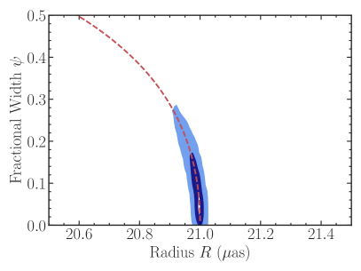
Figure 5 shows the 68% and 95% credible intervals for the two primary parameters of the model: the radius of the ring and its fractional width . The values of these parameters and their correlation can be understood completely in terms of the location of the minimum in the visibility amplitudes that occurs at a baseline length of G (see Fig. 4). The red dashed line in Figure 5 shows the expected correlation between fractional width and radius for all symmetric rings that have the first minimum of the visibility amplitude occurring at that baseline length. (Note that, for the purposes of this figure, which requires a relative accuracy of better than 1 part in 1000, we used the numerical solution for the correlation between fractional width and ring radius and not the analytic approximation [17]).
Marginalizing the posterior over all model parameters other than the radius results in , which corresponds to a fractional uncertainty of 0.1%. This is a surprisingly small uncertainty given that there are 152 visibility amplitude and 119 closure phase data points, the uncertainty of each complex visibility was set to 10%, and the model has only a handful of free parameters. For comparison, if this was a power-law model in visibility, i.e., , and there were equidistant data points in between a minimum baseline G and a maximum baseline G, all with fractional uncertainty , then the uncertainty in the coefficient of that model would be
| (18) | |||||
i.e., an order of magnitude larger.
The fact that the uncertainties in the measurement of one of the key model parameters is substantially smaller than what one might expect suggests that the model predictions for at least some of the data points depend very strongly on that model parameter. This might be viewed naively as good news, since it allows for strong constraints to be placed on model parameters with only marginal uncertainties in the data. However, it also implies that the inferred uncertainties in the model parameters rely extremely strongly on the ability of the model to predict accurately the salient features of the visibility data. The latter is unlikely to be true when we are using simple geometric models (e.g., crescent shapes) to fit visibility data that describe images of turbulent accretion flows around black holes.
4 The Role of Influential Data Points
The example discussed in the previous section demonstrates that a very small number of data points near the location of salient features in the visibility data obtained with an interferometer such as the EHT have an uneven degree of influence on the measurements and uncertainties of model parameters. This is true even for our example that was based on synthetic data generated by the actual crescent model, with the same fractional uncertainties for each data point. The effect gets exacerbated when the data points have different uncertainties (i.e., they are heteroscedastic) and the actual data are only broadly described by the simple geometric model that we try to fit to them, as is the case in real applications to EHT data.
Quantifying the degree of influence of different data points on model fitting has been extensively explored in both the frequentist (see, e.g., Cook 1977, 1979) and the Bayesian frameworks (see, e.g., Millar & Stewart 2007). Both approaches generate very similar outcomes as they identify two types of influential data points. The first type are the outliers, i.e., the ones that deviate from model predictions by a degree that is statistically inconsistent with the uncertainties. The presence of such data points alters the inferred uncertainties in the model parameters. The second type are the subset of data points that depend substantially more strongly on the model parameters than the remaining data points and, therefore, exert uneven leverage in determining the best-fit values of the model parameters.
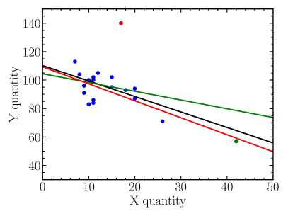
A toy example with both types of data points is shown in Figure 6, where a linear model is fit to the data set used in the Bayesian analysis of Millar & Stewart (2007); the best-fit line is shown in black and its parameters are shown in Table 1. The red data point is a clear outlier. Removing it introduces only a small change to the parameters of the best-fit line (red curve); however, removing just that single point reduces the inferred uncertainties of the model parameters by as much as a factor of 2. The green data point appears at a large horizontal distance from the other data points and, therefore, exerts substantial leverage in determining the model parameters. Removing the green point changes substantially the best-fit model parameters, i.e., leads to a best-fit line (green curve) that is significantly flatter than when the full data set is used. This toy example demonstrates how removing even a single influential point changes substantially the parameters of the best-fit model and their uncertainties. For this reason, identifying such influential points for EHT data is critical in assessing the robustness of the results of model fits.
| Data Set | slope | y-intercept |
|---|---|---|
| Full Data Set | -1.09 0.40 | 110.2 6.5 |
| Red Point Excluded | -1.19 0.24 | 109.3 4.0 |
| Green Point Excluded | -0.61 0.66 | 104.4 9.2 |
4.1 Identifying Influential Data Points
In order to quantify and formally measure the influence of each data point on results of model fiting, we follow the Bayesian approach of Millar & Stewart (2007). The qualitative idea is to measure the change in the information content of the resulting posterior when we artificially broaden (or shrink) the likelihood that corresponds to each one of the data points. If this change is similar among all data points, this would imply that all of them have similar influences on the result. If, on the other hand, this change is substantially larger for some of the data points, we will conclude that the latter have high influence on the result.
We define the quasi-likelihood data as the likelihood of obtaining the data set from a particular set of model parameters but with the likelihood of the th data point having been broadened by a factor , i.e., (cf. eq. [9])
| (19) |
If the likelihood of the th data point is a Gaussian with dispersion , the contribution of this data point to the total likelihood in equation (19) is also a Gaussian but with a dispersion equal to . When , the -th data point does not contribute to the determination of the best-fit parameters.
Using this quasi-likelihood, we define a new quasi-posterior by effectively elevating the parameter to a model parameter as (cf. eq. [8])
| (20) |
here we have incorporated the prior on the model parameters. When , the above quasi-posterior is equal to the true posterior (8). In order to quantify the change in the information content of the posterior when we artificially change the likelihood of the -th data point, i.e., when we set , we use the Kullback-Leibler (KL) divergence
| (21) |
By definition, when , the KL divergence is equal to zero as is its first derivative with respect to , under normal conditions (Millar & Stewart, 2007). The second derivative of the KL divergence with respect to offers the lowest-order non trivial measure of the variation with . After some simple manipulations, the second derivative becomes
| (22) |
This is the well known result that the curvature of the KL-divergence is equal to the Fisher information with respect to the relevant parameter (here ).
Using equations (19), (20), and (22) we obtain
| (23) |
This is the measure of the influence of the -th data point on the results and it is equal to the variance of the log-likelihood of this data point across the space of the model parameters. Millar & Stewart (2007) suggest as a normalized measure of the influence of the -th data point the ratio
| (24) |
where the denominator involves the combined log-likelihood for all data points. In general, the sum will not be equal to unity, because the individual likelihoods may be correlated. Also note that Spiegelhalter et al. (2002) (see also Gelman et al. 2013) identified the denominator of equation (24) as a measure of the complexity of the model given the data, i.e., of the effective number of degrees of freedom. Among a set of data points, those with will be the ones with disproportionate influence on the result of the model fitting.
4.2 Influential Data Points in Crescent Images
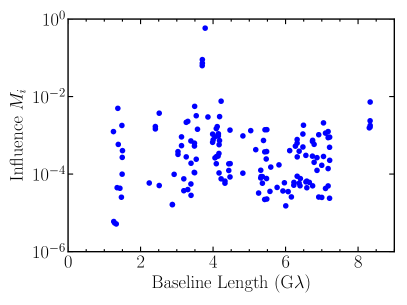
In this subsection, we apply the formalism we developed in §4.1 to the test problem of fitting crescent models to interferometric data that we discussed in §3 (see Figures 4-5). Figure 7 shows the influence (eq. [24]) of each of the visibility-amplitude data points on the result as a function of its baseline length. For the vast majority of data points, . This is not true, however, for the three data points that lie at the first minimum of the visibility amplitude curve. The large values of for these three data points, which are several orders of magnitude larger than the others, demonstrate their disproportionate influence on the result. Indeed, the fact discussed in §3 that the best-fit values of and correlations between the inferred radius and fractional width of the crescent are determined almost entirely by the location of the first minimum in the visibility amplitude data is directly related to this disproportionate influence. Note that the influence values of the corresponding closure-phase data do not single out any additional influential points for this synthetic data set.
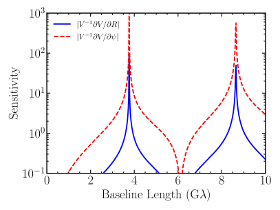
In order to understand the origin of the disproportionate influence of the data points near the visibility minima on the outcome of the model comparison, we explore the sensitivity of the inference of model parameters on the location of data points of the plane. As we did above, we focus on the visibility amplitude data, although similar considerations apply to the closure phase data as well. The sensitivity in the inference of a particular model parameter on the measurement at the location () of a given data point will depend on the uncertainty of the measurement (the higher the uncertainty the weaker the sensitivity) and on the derivative of the model prediction with respect to , evaluated at the location of the data point, i.e.,
| (25) |
This term can be recognized as the contribution of the -th data point on the Cramér-Rao bound of the uncertainty in the inference of the -model parameter. In the last expression, we have normalized the measurement uncertainty of each data point by the model predictions in order to be consistent with our synthetic data that have constant fractional measurement uncertainties. With this normalization, a sensitivity value of unity implies that making, e.g., a change of 1% to the model parameter will cause a change of 1% to the model prediction.
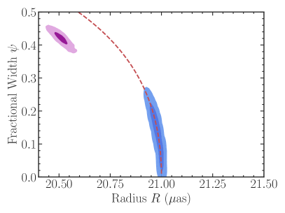
Figure 8 shows the sensitivity of inferring the radius and fractional width of the symmetric ring model using data points with constant fractional uncertainties, as a function of the baseline length of each data point. As expected, both sensitivity curves show very strong peaks near the locations of the minima in the visibility amplitude. Moreover, the inference of the fractional width of the ring has a higher sensitivity on the measurements than the inference of its radius. The location and magnitude of the peaks in these two sensitivity curves match the locations and relative magnitudes of the influence of the various data points shown in Figure 7.
To illustrate the potential biases introduced by the disproportionate influence of a small number of data points on the model parameters, we generate a new set of synthetic data from the ring model with the same parameters and coverage as those discussed in §3 and shown in Figures 3-5. We add to this ring model, however, a single point source at the center of the image that carries a flux of only 0.02 Jy. This is about 1.5% of the total flux of the image and effectively adds a constant to all visibility amplitudes, thus disproportionately affecting the complex visibilities of the data points near the minima in the visibility amplitude curve. The change introduced to the complex visibilities of the vast majority of the remaining data points is within their statistical uncertainties. We then attempt to fit this new synthetic data set with a crescent model that does not include this weak point source. The goal of this test is to simulate the outcome of trying to fit a simple model to an image that has marginally more complex structures than the model allows.
The result for the radius and fractional width for this revised data set are shown in Figure 9. Even though the addition of the weak point source affects only a handful of interferometric data points, the high degree of influence of these data points causes a bias to the inferred model parameters to a degree that is substantially larger than the formal uncertainties from the fitting process. The correlated credible levels for the two parameters do not include the ring parameters that were assumed in the synthetic data. They fall near but not on the expected correlation shown in the red dashed line, given the location of the minimum in the visibility amplitude. As expected from our discussion of the sensitivity of the various model parameters on the measurements, the bias introduced to the fractional width is particularly large (0.4 instead of 0.1 of the underlying image) and is substantially larger than the bias in the radius of the ring.
Note that, in the synthetic dataset we used in these examples, we have set the uncertainties of all data points equal to the same fractional value (10%). This is not the case for the real EHT data, which are widely heteroscedastic; the signal-to-noise ratio for some ALMA baselines can be as large as 300, whereas for some other baselines involving smaller telescopes it is equal to only a few (see Event Horizon Telescope Collaboration et al. 2019c). In this case, the combination of the leverage of each data point (because of its location) and its signal-to-noise ratio will determine its influence: data points with high signal-to-noise ratios in locations of high leverage will have the largest influence. We will explore this more realistic case in §6.
5 The Effect of Sparse Coverage
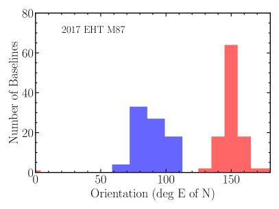
A second important feature of the EHT data that affects the outcome of fitting theoretical models to them is the sparse coverage of the interferometric plane (see, e.g., Fig 3). As Figure 10 shows, in the current form of the array, most of the EHT baselines lie primarily along N-S and E-W orientations, with substantial gaps between them, at all baseline lengths. This preferential orientation of the baselines can introduce strong biases in some of the inferred parameters of models that are fit to the EHT data, as we will now show.
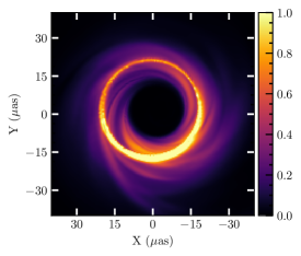
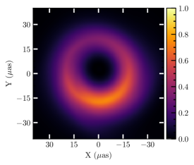
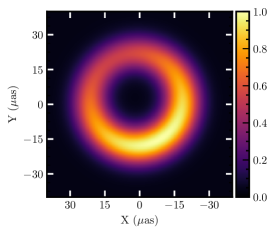
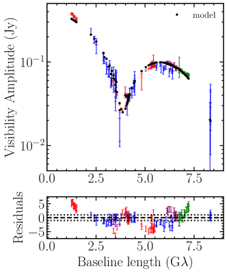
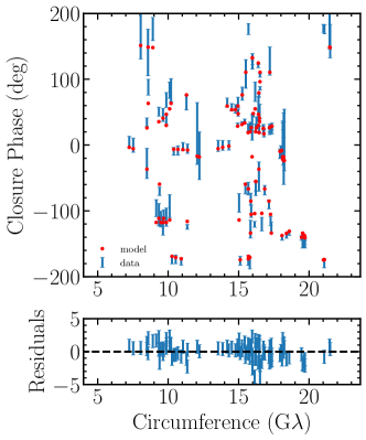
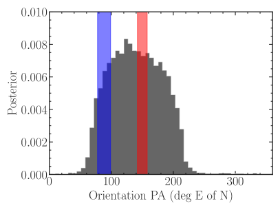
Figure 11 shows the marginalized posterior over position angle of the crescent model fit to the synthetic data introduced in §3 (see also Fig. 3-5); for consistency with earlier literature, we report the position angle in degrees East of North, i.e., as . Even though the underlying image in this example is a fully symmetric ring with no preferred orientation, the posterior over orientation angle peaks at values similar to those of the primary orientations of the EHT baselines. This is a direct consequence of the projection-slice theorem, which states that a cross section of a 2-dimensional Fourier transform along a particular orientation is equal to the Fourier transform of the projection of the image along the same orientation. As discussed in §3, the analytic crescent model has a preferred orientation along which the cross section of the Fourier transform is independent of the degree of symmetry () of the crescent. In other words, crescents that are mildly different than the symmetric ring (i.e., with a mild asymmetry) will lead to the same predictions as the symmetric model for the observations along the EHT baselines as long as their symmetry axes are lined up with the orientations of the baselines. When marginalized over all other model parameters, the large volume in the space of models occupied by asymmetric crescents that are aligned with the EHT baselines and can reproduce the data within their uncertainties gives rise to a posterior over orientation that is aligned with the EHT baselines.
It is important to emphasize here that not only crescent models but also quasi-analytic (see, e.g., Broderick et al. 2009) and even GRMHD model images (see, e.g., Event Horizon Telescope Collaboration et al. 2019e) of black-hole shadows have intrinsic symmetry axes dictated by the spin of the black hole and the brightness asymmetry introduced by Doppler effects. As a result, similar considerations apply when fitting such models to the EHT data. Moreover, the synthetic dataset we used here is characterized by the same fractional uncertainties for all data points, which is not realistic. In a more realistic situation, a complex image of a black hole will be observed with the EHT and will result in a heteroscedastic dataset. In this case, it will be a complex combination of the preferred orientations of the baselines with the largest signal-to-noise ratio, of the underlying symmetry and orientation of the image, as well as of the symmetry properties of the model that will determine potential biases in the posterior over orientation angle.
6 Application to Synthetic EHT Data
In order to explore a more realistic situation that includes small-scale structure, as well as realistic measurement uncertainties, we used two of the GRMHD+GR Radiative Transfer simulations calculated by Chan et al. (2015), but for parameters relevant to the M87 black hole. In particular, we used one simulation with the Magnetically Arrested Disk (MAD) field structure (Narayan et al., 2012). We set the mass of the black hole to , the spin of the black hole to , the inclination of the observer to , the position angle of the black-hole spin axis to 290∘ East of North, and the electron temperature to follow a plasma -dependent prescription with (see Event Horizon Telescope Collaboration et al. 2019e). We created images at 1.3 mm using the GPU-accelerated GRay algorithm (Chan et al., 2013) and calculated angular sizes in the sky for a distance of 16.8 Mpc. Finally, we generated synthetic EHT data from images generated with these simulations, with a coverage and thermal noise levels that are identical to those of the 2017 EHT observations of M87 (Event Horizon Telescope Collaboration et al. 2019c; see Fig. 3 for the coverage).
In the following subsection, we discuss a number of cases that correspond to different morphologies of the underlying images.
6.1 Images with Dominant Crescent Structures
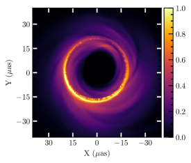
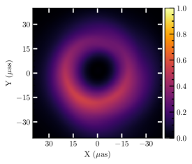
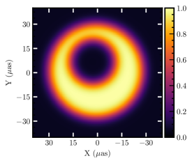
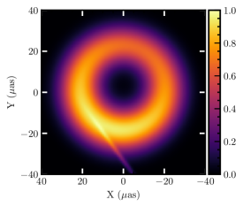
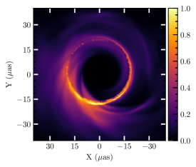
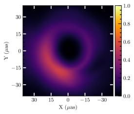
The low inferred inclination of the black-hole spin in M87 substantially reduces the brightness asymmetry that is caused by the Doppler effect (compare, e.g., with the case of high-inclination simulations for Sgr A* reported in Chan et al. 2015). As a result, if the emission is highly localized near the black-hole horizon, the resulting image will be dominated by a crescent structure with mild asymmetry. An example of such a snapshot from our MAD simulation is shown in the left panel of Figure 12. The North-South brightness asymmetry in this snapshot is 2:1, similar to what is inferred in the M87 image. The middle panel of the same figure shows the same snapshot but filtered with a cutoff baseline of 15 G to suppress structures that are not accessible to the EHT array; for this and the following figures, this is achieved by using an Butterworth filter (see Psaltis et al. 2020).
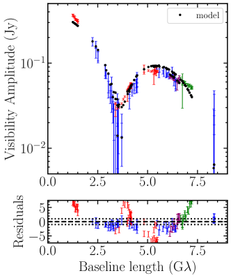
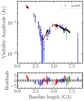
Figure 13 shows the synthetic data for visibility amplitudes and closure phases generated from this image. For the assumed parameters of the black hole, the radius of the shadow is equal to 18.7 as and, for an image dominated by an infinitesimal bright ring surrounding the shadow, the first minimum in the visibility amplitude is expected at a baseline length of G. The synthetic data show instead a visibility amplitude minimum at a baseline length of G, which corresponds to a radius of the emitting region of as, signifying a broader emission region.
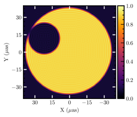
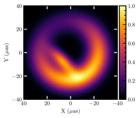
Figure 13 also shows the best-fit crescent model that we obtained after running MARCH for 50 million steps and 40 replica temperatures. For the purposes of this test, we allowed for the crescent image to have softer edges by multiplying the complex visibilities of the model (eq. [10]) with a Gaussian function, which is equivalent to convolving the crescent image by the corresponding Gaussian kernel. The right panel of Figure 12 shows the image that corresponds to the best-fit model parameters. Clearly, when the underlying image is dominated by a crescent structure, then fitting a simple crescent model to synthetic EHT data results in only small residuals and a model image that closely matches the properties of the one used to generate the synthetic data.
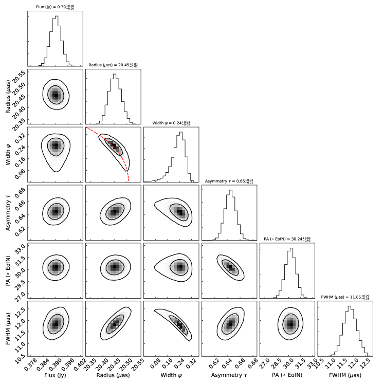
Figure 14 shows the posteriors of the model parameters. The very high signal-to-noise ratio of the data, which exceeds 100 for some of the data points, together with the small number of model parameters, leads to highly constrained values for the latter. Large correlations can be seen primarily between two pairs of model parameters. The posteriors in the fractional width and the radius of the crescent are correlated according to equation (17), as their values are primarily determined by the baseline length of the first minimum in the visibility amplitude222The definition of the fractional width as would introduce an anticorrelation but this explains neither the shape nor the range of values of the correlated posteriors.. At the same time, the posteriors in the FWHM of the broadening Gaussian kernel and the fractional width of the crescent are anticorrelated because the same effective broadening of the crescent can be achieved by either increasing the fractional width of the crescent or by broadening it by a wider Gaussian kernel.
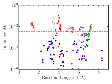
Figure 15 shows the relative influence that each of the synthetic data points with realistic uncertainties exerts on the inference of the model parameters, calculated using equation (24). In order to separate the two types of influential data points (i.e., those with intrinsically large leverage versus the outliers that are not well described by the model), we have used filled and open circles to denote the data points for which the difference between the measurement and the model prediction is less than or more than 2.5 times the measurement uncertainty, respectively. We have also color-coded the data points as in Figure 3 to show the orientations of the various baselines. As expected from the discussion in §4, the data points near the minimum of the visibility amplitude at G are described well by the model and have high leverage in determining the model parameters. In contrast, a number of data points exist at various baselines that are not described well by the model (i.e., they have large residuals) but exert substantial influence in determining the model parameters because they are outliers. In this case of a realistic image, which is not described adequately by a simple crescent model, and of heteroscedastic data, the posteriors of the model parameters are determined by a combination of the influence of data points of high leverage and of the outliers.
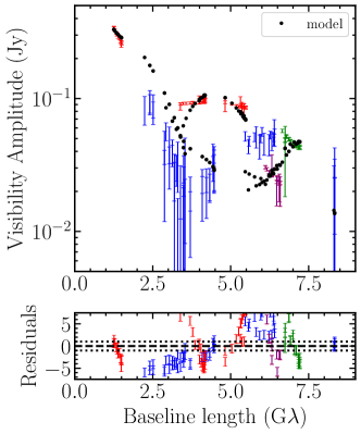
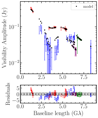
The fact that an image appears to be dominated by a crescent structure does not mean that the resulting synthetic data will always be well described by a crescent model. This is demonstrated in Figure 16, which shows a snapshot with what appears to be a dominant crescent structure. However, fitting the resulting synthetic data with a crescent model results in substantial residuals (see left panel of Fig. 17) and the corresponding best-fit image does not match the width or the orientation of the original image (see lower left panel of Fig. 16).
It is tempting to try to improve the quality of the fit by adding elliptical Gaussian components to the crescent model. Adding even a single such elliptical Gaussian increases the number of model parameters from 6 (see Fig. 14) to 12, with the additional six parameters being the centroid positions along the two axes of the Gaussian component, its major and minor axes, its position angle, and its flux. This large increase in the number of model parameters indeed leads to substantially smaller residuals, as can be seen in the right panel of Figure 17.
Comparing the best-fit image to the original snapshot from the simulation (see lower right panel of Fig. 16) reveals that the additional Gaussian component seems to be adding flux at the lower-left quadrant of the image that has additional structure. However, it is extremely narrow and its minor axis in the image domain (i.e., the major axis in the visibility domain) is aligned with the orientation of the green baselines. This is not surprising, given that the main utility of the additional elliptical Gaussian component in this particular example has been to reduce the residuals along the red and green color-coded baselines, which have the highest signal-to-noise ratios, without affecting substantially the blue color-coded ones, which have lower signal-to-noise ratios and were well described by the simple crescent model (see Fig. 3 for the color code of the baselines). The size, asymmetry, and orientation of the additional Gaussian component is simply an artifact of the sparse coverage of the EHT array and the orientations of its baselines.
Nevertheless, even though the properties of the additional Gaussian component are not reliable, its presence allowed the best-fit crescent model to have a width and an orientation that more closely matches that of the original snapshot compared to the best-fit model without this extra component. In both examples described in this subsection, the dominant crescent shapes in the images caused deep minima in the visibility amplitudes at baselines G and, for this reason, the inferred sizes of the crescents are comparable to the true values.
6.2 Images with Sub-Dominant Crescent Structures
Figure 18 shows a third example of a snapshot from a MAD simulation with characteristics that are frequently encountered. In this example, there is substantial structure beyond the simple crescent shape that persists even after we filtered the image with the Butterworth filter in order to suppress visually the structures that are not accessible to the EHT data.
The synthetic data from this snapshot (Fig. 19) indeed do not show the characteristic ringing structure with pronounced deep minima and the overlapping secondary maxima of the crescent shapes along all orientations. It is, therefore, expected that fitting a simple broadened crescent model to the synthetic data (left panel of Fig. 19) leaves substantial residuals at all baselines. The resulting best-fit image (lower-left panel of Fig. 18) does not match any of the structures in the image from which the synthetic data were generated.
Adding an additional Gaussian component to the model substantially improves the quality of the fit and reduces the residuals, especially along the red- and green-baselines that have the data with the highest signal-to-noise ratios (right panel of Fig. 19). The best-fit image (lower right panel of Figure 18), however, shows structures that again do not match those of the image from which the synthetic data were generated. The width of the crescent shape is reasonable but neither its orientation nor its size are correct. Moreover, as in Fig. 16 in the last example discussed in the previous subsection, the minor axis of the additional Gaussian component in the image domain (i.e., the major axis in the visibility domain) is aligned with the orientation of the green baselines.
7 Conclusions
In this paper, we introduced MARCH, a new Markov Chain Monte Carlo algorithm with parallel tempering for fitting theoretical models to the interferometric data from the Event Horizon Telescope. We then used this algorithm to explore the biases in the inferred parameters of crescent models that we fit to synthetic EHT data based on images from GRMHD simulations. We explored, in particular, biases that are introduced by the uneven influence of data points, the heteroscedastic nature of the EHT data, and the sparse coverage of the interferometric plane with the EHT baselines.
When the images are dominated by strong crescent structures, we find that there are a number of salient features in the interferometric data, such as a deep minimum in the visibility amplitude at a baseline length determined primarily by the size of the image. Data obtained in the vicinity of such salient features exert a disproportionate influence on the values of the inferred model parameters, artificially reducing the widths of their posteriors.
When the underlying images have structures that are not well characterized by crescent shapes, fitting crescent models to synthetic EHT data reveals substantial residuals, as expected. Attempting to ameliorate these residuals by adding compact (e.g., Gaussian) components to the models may improve the quality of the fit and reduce the residuals. However, the properties of the additional components are strongly biased by the locations and orientations of the EHT baselines and are not trustworthy. Such Gaussian components with similarly large aspect ratios and orientations were deemed necessary to fit the actual M87 data observed in 2017 with the EHT (see Fig. 5 of Event Horizon Telescope Collaboration et al. 2019f).
When the underlying image has a high degree of symmetry, the sparse baseline coverage of the EHT array often biases even the inferred overall orientation of the underlying image to align with the orientations of the primary baselines (see, e.g., Fig. 11). If we were to match the features of a crescent model with those of a snapshot from a GRMHD simulation, we would identify the ”orientation” of the crescent image (which measures the orientation of displacement between the outermost, positive disk and the innermost, negative one) with the perpendicular orientation to that of the black-hole spin. Figure 11 shows that the orientations of a crescent model that was fit to synthetic EHT data of a symmetric structure appear to get biased towards a position angle of EofN. This would imply a bias in the inferred orientation of the black-hole spin towards an orientation EofN, which is very similar to the value with the highest posterior inferred from fitting crescent models to the 2017 EHT data and casts doubt on that inference (see, e.g., Figure 9 of Event Horizon Telescope Collaboration et al. 2019e).
In all cases, the robust detection of salient features leads to the determination of the characteristic sizes of crescent images that are within a small fractional distance from (albeit often statistically inconsistent with) the true sizes of the underlying images. When such salient features are detected, as was the case with the 2017 EHT data on M87, the size of the black-hole shadow and, hence, of the black-hole mass is not significantly biased. In order to obtain accurate measurements of additional aspects of the image, such as its orientation, asymmetry, and presence of additional structures, requires a more complete coverage of the space with the addition of more stations in the EHT array. A number of such stations have been introduced since the 2017 observations, such as the GLT telescope in Greenland, the 12m telescope on Kitt Peak, and NOEMA in the French Alps, which will help substantially in alleviating the biases introduced by the sparse baseline coverage of the current EHT.
References
- Akiyama et al. (2017a) Akiyama, K., Kuramochi, K., Ikeda, S., et al. 2017a, ApJ, 838, 1
- Akiyama et al. (2017b) Akiyama, K., Ikeda, S., Pleau, M., et al. 2017b, AJ, 153, 159
- Benkevitch et al. (2016) Benkevitch, L., Akiyama, K., Lu, R., Doeleman, S., & Fish, V. 2016, arXiv e-prints, arXiv:1609.00055
- Berger et al. (2012) Berger, J. P., Malbet, F., Baron, F., et al. 2012, A&A Rev., 20, 53
- Blackburn et al. (2019) Blackburn, L., Pesce, D. W., Johnson, M. D., et al. 2019, arXiv e-prints, arXiv:1910.02062
- Broderick et al. (2009) Broderick, A. E., Fish, V. L., Doeleman, S. S., & Loeb, A. 2009, ApJ, 697, 45
- Broderick et al. (2016) Broderick, A. E., Fish, V. L., Johnson, M. D., et al. 2016, ApJ, 820, 137
- Chael et al. (2018) Chael, A. A., Johnson, M. D., Bouman, K. L., et al. 2018, ApJ, 857, 23
- Chael et al. (2016) Chael, A. A., Johnson, M. D., Narayan, R., et al. 2016, ApJ, 829, 11
- Chan et al. (2013) Chan, C.-k., Psaltis, D., & Özel, F. 2013, ApJ, 777, 13
- Chan et al. (2015) Chan, C.-K., Psaltis, D., Özel, F., Narayan, R., & Sadowski, A. 2015, ApJ, 799, 1
- Christian & Psaltis (2019) Christian, P., & Psaltis, D. 2019, arXiv e-prints, arXiv:1909.04681
- Clark (1980) Clark, B. G. 1980, A&A, 89, 377
- Cook (1977) Cook, R. D. 1977, Technometrics, 19, 15
- Cook (1979) —. 1979, J. Amer. Stat. Assoc., 73, 365
- Dexter et al. (2009) Dexter, J., Agol, E., & Fragile, P. C. 2009, ApJ, 703, L142
- Earl & Deem (2005) Earl, D. J., & Deem, M. W. 2005, Physical Chemistry Chemical Physics (Incorporating Faraday Transactions), 7, 3910
- Event Horizon Telescope Collaboration et al. (2019a) Event Horizon Telescope Collaboration, Akiyama, K., Alberdi, A., et al. 2019a, ApJ, 875, L1
- Event Horizon Telescope Collaboration et al. (2019b) —. 2019b, ApJ, 875, L2
- Event Horizon Telescope Collaboration et al. (2019c) —. 2019c, ApJ, 875, L3
- Event Horizon Telescope Collaboration et al. (2019d) —. 2019d, ApJ, 875, L4
- Event Horizon Telescope Collaboration et al. (2019e) —. 2019e, ApJ, 875, L5
- Event Horizon Telescope Collaboration et al. (2019f) —. 2019f, ApJ, 875, L6
- Falcke et al. (2000) Falcke, H., Melia, F., & Agol, E. 2000, ApJ, 528, L13
- Foreman-Mackey et al. (2013) Foreman-Mackey, D., Hogg, D. W., Lang, D., & Goodman, J. 2013, PASP, 125, 306
- Gelman et al. (2013) Gelman, A., Hwang, J., & Vehtari, A. 2013, arXiv e-prints, arXiv:1307.5928
- Högbom (1974) Högbom, J. A. 1974, A&AS, 15, 417
- Honma et al. (2014) Honma, M., Akiyama, K., Uemura, M., & Ikeda, S. 2014, PASJ, 66, 95
- Jennison (1958) Jennison, R. C. 1958, MNRAS, 118, 276
- Kamruddin & Dexter (2013) Kamruddin, A. B., & Dexter, J. 2013, MNRAS, 434, 765
- Kim et al. (2016) Kim, J., Marrone, D. P., Chan, C.-K., et al. 2016, ApJ, 832, 156
- Lu et al. (2018) Lu, R.-S., Krichbaum, T. P., Roy, A. L., et al. 2018, ApJ, 859, 60
- Medeiros et al. (2017) Medeiros, L., Chan, C.-k., Özel, F., et al. 2017, ApJ, 844, 35
- Medeiros et al. (2018) —. 2018, ApJ, 856, 163
- Millar & Stewart (2007) Millar, R. B., & Stewart, W. S. 2007, Bayes. Anal., 2, 365
- Mościbrodzka et al. (2014) Mościbrodzka, M., Falcke, H., Shiokawa, H., & Gammie, C. F. 2014, A&A, 570, A7
- Mościbrodzka et al. (2009) Mościbrodzka, M., Gammie, C. F., Dolence, J. C., Shiokawa, H., & Leung, P. K. 2009, ApJ, 706, 497
- Narayan & Nityananda (1986) Narayan, R., & Nityananda, R. 1986, ARA&A, 24, 127
- Narayan et al. (2012) Narayan, R., SÄ dowski, A., Penna, R. F., & Kulkarni, A. K. 2012, MNRAS, 426, 3241
- Özel et al. (2000) Özel, F., Psaltis, D., & Narayan, R. 2000, ApJ, 541, 234
- Psaltis et al. (2015) Psaltis, D., Özel, F., Chan, C.-K., & Marrone, D. P. 2015, ApJ, 814, 115
- Roelofs et al. (2017) Roelofs, F., Johnson, M. D., Shiokawa, H., Doeleman, S. S., & Falcke, H. 2017, ApJ, 847, 55
- Spiegelhalter et al. (2002) Spiegelhalter, D. J., Best, N. G., Carlin, B. P., & van der Linde, A. 2002, Journal Royal Stat. Soc. B., 64, 583
- Thiébaut (2009) Thiébaut, E. 2009, New A Rev., 53, 312
- Thompson et al. (2017) Thompson, A. R., Moran, J. M., & Swenson, George W., J. 2017, Interferometry and Synthesis in Radio Astronomy, 3rd Edition, doi:10.1007/978-3-319-44431-4