Abstract

Network autocorrelation models have been widely used for decades to model the joint distribution of the attributes of a network’s actors. This class of models can estimate both the effect of individual characteristics as well as the network effect, or social influence, on some actor attribute of interest. Collecting data on the entire network, however, is very often infeasible or impossible if the network boundary is unknown or difficult to define. Obtaining egocentric network data overcomes these obstacles, but as of yet there has been no clear way to model this type of data and still appropriately capture the network effect on the actor attributes in a way that is compatible with a joint distribution on the full network data. This paper adapts the class of network autocorrelation models to handle egocentric data. The proposed methods thus incorporate the complex dependence structure of the data induced by the network rather than simply using ad hoc measures of the egos’ networks to model the mean structure, and can estimate the network effect on the actor attribute of interest. The vast quantities of unknown information about the network can be succinctly represented in such a way that only depends on the number of alters in the egocentric network data and not on the total number of actors in the network. Estimation is done within a Bayesian framework. A simulation study is performed to evaluate the estimation performance, and an egocentric data set is analyzed where the aim is to determine if there is a network effect on environmental mastery, an important aspect of psychological well-being.

KEY WORDS: Actor attributes; Bayesian estimation; Social influence; Spatial autoregressive model.

1 Introduction

Network autocorrelation models can help capture complex dependencies in individual level data and can also estimate how and to what extent an individual’s network influences that individual’s attributes or behaviors. Fujimoto et al. (2011) describes the network autocorrelation model as “a workhorse for modeling network influences on individual behavior.” Wang et al. (2014) states “The network autocorrelation model has some clear advantages over other conventional approaches (e.g., egocentric or dyadic) in that it simultaneously accommodates network effects and individual attributes.” This class of models has been used for decades in a variety of contexts, such as determining the network effect on gender roles in labor (White et al., 1981), educational and occupational aspirations (Duke, 1991), U.S. interstate commodity flows (Chun et al., 2012), policy influence (Carpenter et al., 1998), task performance (Carr & Zube, 2015), and phylogenetics (Björklund, 1990).

Network autocorrelation models describe stochastic data generating processes using the joint distribution of all actor attributes given the network structure. This is both a benefit and a curse. The positive aspect of this, and indeed the motivation for employing such an approach, is that by jointly modeling all actors in the network, the complex dependence structure is explicitly modeled, and social influence can be directly quantified and estimated. The downside is that to utilize such a model, one needs to collect data on all actors in the network. This can be a problem for (at least) three reasons. First, often times the network is simply too large to sample (Granovetter, 1976), or there are monetary constraints to obtaining data on all the actors of the network. Second, the actors of the network may not be easily accessible to the researchers, especially if the network is defined by controversial or illegal behaviors. Third, the boundary of the network may not be identifiable. For example, suppose one wishes to know the network effect of peers on adolescent behaviors. Is the network of interest defined by all adolescents in a particular class or school? Or perhaps it can be defined by some on-line social media platform? Or perhaps it is all adolescents in a particular city, state, or country? Doreian (1989) makes the statement, which still holds true today, “locating [a network’s] boundaries remains a persistent and vexing problem.”

Researchers often avoid the difficulty of collecting data on all actors of the network by obtaining a subsample of the actors and focusing on the ties involving the sampled actors. The resulting data is referred to as egocentric network data. This type of data can be collected in a variety of ways, such as a simple random sample, targeted sampling, snowball sampling, respondent-driven sampling, etc (see, e.g., Heckathorn, 1997). Egocentric network analyses have been used to study interorganizational collaborations (Ahuja, 2000), health behaviors (O’Malley et al., 2012), personal and group communication (Fisher, 2005), contraceptive use (Behrman et al., 2003), support network after cancer diagnoses (Ashida et al., 2009), and many others.

The use of egocentric data has been limited primarily to the study of either dyadic relationships or structural/positional measures of the entire network (Provan et al., 2007). Methods to study actor attributes using egocentric data are more limited in scope; this type of analysis is often done in an ad hoc manner by using as a covariate some summary statistic of the egos’ personal networks such as density, network size, or an average of some alter attribute.

This paper proposes a novel method that adapts the network autocorrelation model to egocentric network data. The proposed method is derived directly from the joint distribution of all actors in the network, even if the boundary of the network is unknown or ill-defined, and thus incorporates the complex dependence structure of the data induced by the network rather than simply using ad hoc measures of the network in the mean structure. Estimation is done within a Bayesian framework.

Section 2 describes the proposed methodology. Section 3 describes a simulation study that compares the performance of the proposed method with OLS estimators which ignore the network effect and with estimators using the entire network data. Section 4 shows the results from applying the proposed method to an egocentric data set of adults in a rural southeastern Iowa town, with the goal of determining if there is a network effect on environmental mastery. Section 5 provides a brief discussion.

2 Methods

Suppose that we wish to make inference regarding a graph augmented with actor attributes. We may view this as a triple ${\cal G}=({\cal V},{\cal E},{\cal A})$; ${\cal V}$ is the set of vertices, or actors, of the network, ${\cal E}$ is the set of edges, or relations, between the vertices, and ${\cal A}$ is the set of actor attributes on ${\cal V}$. We will denote $|{\cal V}|$, the number of actors, by $n$. Typically one may represent ${\cal E}$ by an adjacency matrix $A$, where the $i^{th}$ row $j^{th}$ column entry of $A$ is 1 if there is an edge between actors $i$ and $j$ and 0 otherwise. The actor attributes ${\cal A}$ can be partitioned into the $n\times 1$ response variable vector $\boldsymbol{y}$ and the $n\times p$ matrix of covariates $X$. The goal is to try to determine how the covariates $X$ and the network affect the response $\boldsymbol{y}$. This is typically accomplished via network autocorrelation models.

The network autocorrelation model has its genesis in spatial statistics (e.g., Ord, 1975; Doreian, 1980). It was soon borrowed by researchers studying complex network data to great effect (e.g., Dow et al., 1982). There are two variations on a theme, namely, (borrowing nomenclature from Doreian, 1980), the network effects model, given by

$$\boldsymbol{y}= X\boldsymbol{\beta}+\rho A\boldsymbol{y}+\boldsymbol{\epsilon},$$ (1)

and the network disturbances model, given by

$$\boldsymbol{y} =X\boldsymbol{\beta}+\boldsymbol{\nu},$$

$$\boldsymbol{\nu} =\rho A\boldsymbol{\nu}+\boldsymbol{\epsilon},$$ (2)

where $\boldsymbol{\beta}$ is the parameter vector of coefficients, $\rho$ is the coefficient which captures the network effect, and $\boldsymbol{\epsilon}$ is a vector of zero mean independent normal random variables with homogeneous variance $\sigma^{2}$. Note that an equivalent but more concise form of (2) is

$$\boldsymbol{y} =X\boldsymbol{\beta}+\rho A(\boldsymbol{y}-X\boldsymbol{\beta})+\boldsymbol{\epsilon}.$$ (3)

For egocentric data, ${\cal G}$ is only partially observed. Figure 1 illustrates an egocentric network for a small toy data set. The set of actors ${\cal V}$ can be partitioned into the sampled egos ${\cal V}_{e}$, the egos’ alters ${\cal V}_{a}$ (those actors with whom the egos have ties), and all other actors in the network ${\cal V}_{o}$, so that ${\cal V}={\cal V}_{e}\cup{\cal V}_{a}\cup{\cal V}_{o}$. Let $n_{e}$, $n_{a}$, and $n_{o}$ denote the number of egos, the number of the egos’ alters, and the number of remaining actors in the network respectively, so that $n=n_{e}+n_{a}+n_{o}$. We can partition ${\cal E}$ by focusing on the adjacency matrix $A$, specifically

$$A =\begin{pmatrix}A_{e}&A_{ea}&{\bf 0}\\ A_{ea}^{\prime}&A_{a}&A_{ao}\\ {\bf 0}&A_{ao}^{\prime}&A_{o}\end{pmatrix},$$

and similarly we can partition $\boldsymbol{y}$ and $X$ by

$$\boldsymbol{y} =(\boldsymbol{y}_{e}^{\prime},\boldsymbol{y}_{a}^{\prime},\boldsymbol{y}_{o}^{\prime})^{\prime}$$

$$X =(X_{e}^{\prime},X_{a}^{\prime},X_{o}^{\prime})^{\prime},$$

where the subscripts $e$, $a$, and $o$ correspond to the egos, the egos’ alters, and all other actors in the network respectively.

Obviously there are quite a few unknowns here, not the least of which is the number of others $n_{o}$, and hence the size of the network $n$. Specifically, we do not know $\boldsymbol{y}_{a}$, $\boldsymbol{y}_{o}$, $X_{o}$, $A_{a}$, $A_{ao}$, nor $A_{o}$. Trying to directly employ either the network effects or disturbances model is clearly not possible with so much missing data (and quite possibly an unknown amount of missing data). The goal, then, is to capture as much of the information as possible while confining all the unknowns in as few terms as possible. A conditional distribution, rather than the full joint, will then be used, treating these unknown terms as nuisance parameters to be estimated. We first show how to do this for the network effects model, and then in a similar manner show the same for the network disturbances model.

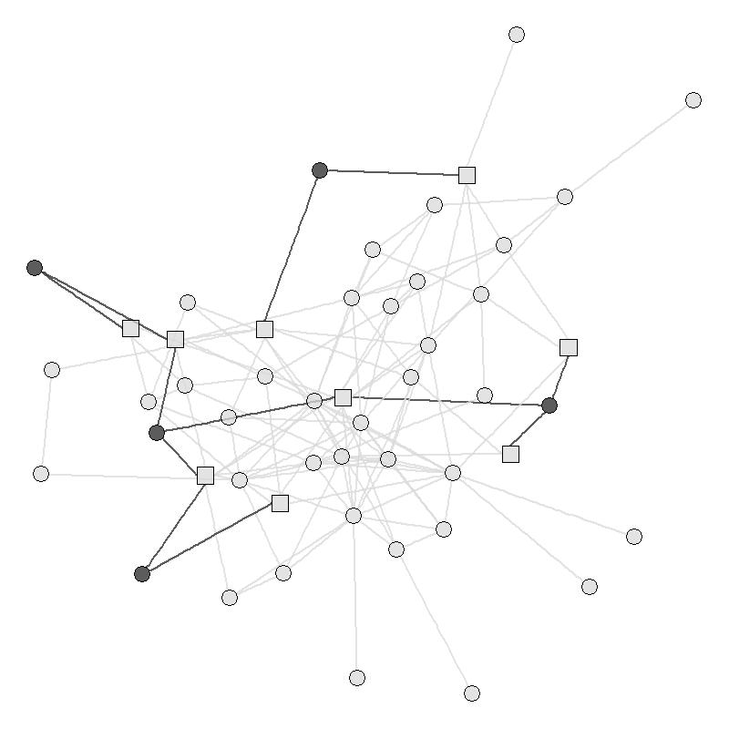
Figure 1: A toy example of an egocentric network, where the dark circles are the sampled egos, the dark edges are the observed egos’ edges, the squares are the alters, and the light gray circles and lines are the unobserved actors and edges respectively.

2.1 Network effects model

We first rewrite (1) into the following three separate equations:

$$\boldsymbol{y}_{e} =X_{e}\boldsymbol{\beta}+\rho A_{e}\boldsymbol{y}_{e}+\rho A_{ea}\boldsymbol{y}_{a}+\boldsymbol{\epsilon}_{e},$$ (4)

$$\boldsymbol{y}_{a} =X_{a}\boldsymbol{\beta}+\rho A_{ea}^{\prime}\boldsymbol{y}_{e}+\rho A_{a}\boldsymbol{y}_{a}+\rho A_{ao}\boldsymbol{y}_{o}+\boldsymbol{\epsilon}_{a}$$ (5)

$$\boldsymbol{y}_{o} =X_{o}\boldsymbol{\beta}+\rho A_{ao}^{\prime}\boldsymbol{y}_{a}+\rho A_{o}\boldsymbol{y}_{o}+\boldsymbol{\epsilon}_{o}$$ (6)

Note that (6) includes no information about the observed data, and so is not used in deriving the conditional likelihood of the observed data. From (4) and (5) we obtain

$$\boldsymbol{y}_{e} =(\rho A_{e}+\rho^{2}A_{ea}A_{ea}^{\prime})\boldsymbol{y}_{e}+(X_{e}+\rho A_{ea}X_{a})\boldsymbol{\beta}$$

$$+\rho^{2}A_{ea}\big{(}A_{a}\boldsymbol{y}_{a}+A_{ao}\boldsymbol{y}_{o}\big{)}+\rho A_{ea}\boldsymbol{\epsilon}_{a}+\boldsymbol{\epsilon}_{e},$$

which implies that

$$\boldsymbol{y}_{e}|\boldsymbol{\alpha} \sim N\Big{(}M_{1}^{-1}\big{[}(X_{e}+\rho A_{ea}X_{a})\boldsymbol{\beta}+\rho^{2}A_{ea}\boldsymbol{\alpha}\big{]},\sigma^{2}M_{1}^{-1}M_{2}M_{1}^{-1}\Big{)},$$

$$M_{1} =I-\rho A_{e}-\rho^{2}A_{ea}A_{ea}^{\prime}$$

$$M_{2} =I+\rho^{2}A_{ea}A_{ea}^{\prime}$$ (7)

where $\boldsymbol{\alpha}=A_{a}\boldsymbol{y}_{a}+A_{ao}\boldsymbol{y}_{o}$. The unknown (nuisance) parameter $\boldsymbol{\alpha}$ can be viewed as the social influence on the alters that cannot be attributed to the egos; we will refer to $\boldsymbol{\alpha}$ as the residual influence effects. This $n_{a}\times 1$ unknown parameter vector succinctly sums up all unknown information about the entire network that pertains to $\boldsymbol{y}_{e}$, and does not depend on $n_{o}$.

2.2 Network disturbances model

For the network disturbances model, we can derive a conditional distribution similar to (7). As before, we first rewrite (3) as three separate equations:

$$\boldsymbol{y}_{e} =X_{e}\boldsymbol{\beta}+\rho A_{e}(\boldsymbol{y}_{e}-X_{e}\boldsymbol{\beta})+\rho A_{ea}(\boldsymbol{y}_{a}-X_{a}\boldsymbol{\beta})+\boldsymbol{\epsilon}_{e}$$ (8)

$$\boldsymbol{y}_{a} =X_{a}\boldsymbol{\beta}+\rho A_{ea}^{\prime}(\boldsymbol{y}_{e}-X_{e}\boldsymbol{\beta})+\rho A_{a}(\boldsymbol{y}_{a}-X_{a}\boldsymbol{\beta})+\rho A_{ao}(\boldsymbol{y}_{o}-X_{o}\boldsymbol{\beta})+\boldsymbol{\epsilon}_{a}$$ (9)

$$\boldsymbol{y}_{o} =X_{o}\boldsymbol{\beta}+\rho A_{ao}^{\prime}(\boldsymbol{y}_{a}-X_{a}\boldsymbol{\beta})+\rho A_{o}(\boldsymbol{y}_{o}-X_{o}\boldsymbol{\beta})+\boldsymbol{\epsilon}_{o}$$ (10)

As before, (10) is irrelevant to the observed egocentric network data and will be disregarded. Combining (8) and (9) yields

$$(I-\rho A_{e}-\rho^{2}A_{ea}A_{ea}^{\prime})\boldsymbol{y}_{e} =(I-\rho A_{e}-\rho^{2}A_{ea}A_{ea}^{\prime})X_{e}\boldsymbol{\beta}$$

$$+\rho^{2}A_{ea}\big{(}A_{a}(\boldsymbol{y}_{a}-X_{a}\boldsymbol{\beta})+A_{ao}(\boldsymbol{y}_{o}-X_{o}\boldsymbol{\beta})\big{)}+\rho A_{ea}\boldsymbol{\epsilon}_{a}+\boldsymbol{\epsilon}_{e},$$ (11)

which implies that

$$\boldsymbol{y}_{e}|\boldsymbol{\alpha} \sim N\Big{(}X_{e}\boldsymbol{\beta}+\rho^{2}M_{1}^{-1}A_{ea}\boldsymbol{\alpha},\sigma^{2}M_{1}^{-1}M_{2}M_{1}^{-1}\Big{)},$$ (12)

where $\boldsymbol{\alpha}=A_{a}(\boldsymbol{y}_{a}-X_{a}\boldsymbol{\beta})+A_{ao}(\boldsymbol{y}_{o}-X_{o}\boldsymbol{\beta})=A_{a}\boldsymbol{\nu}_{a}+A_{ao}\boldsymbol{\nu}_{o}$ and $M_{1}$ and $M_{2}$ are as given previously. Similar to the network effects model, the residual influence effects $\boldsymbol{\alpha}$ can be interpreted as the influence on the residuals of the alters that cannot be attributed to the egos.

2.3 Row Normalization

The choice of $A$ is not always obvious; a notable paper discussing this topic is Leenders (2002). We will limit our discussion to a commonly used transformation of the adjacency matrix, namely row normalization (column normalization can be addressed in nearly exactly the same way). Normalizing the rows such that they each sum to 1 is a practice that has, by some authors, been recommended, and has a long history of implementation (e.g., Ord, 1975; Anselin, 1988).

When the adjacency matrix $A$ has been row normalized, we may think of this as replacing $A$ in (1) and (3) with

$$\begin{pmatrix}D_{e}&{\bf 0}&{\bf 0}\\ {\bf 0}&D_{a}&{\bf 0}\\ {\bf 0}&{\bf 0}&D_{o}\end{pmatrix}A,$$ (13)

where $D_{e}$ is the diagonal matrix whose $i^{th}$ diagonal entry equals the inverse of $\sum_{j=1}^{n}A_{ij}$ (the degree of actor $i$), and similarly for $D_{a}$ and $D_{o}$. From an egocentric network, we only know $D_{e}$. $D_{o}$ is absorbed entirely into residual influence effects $\boldsymbol{\alpha}$, and thus does not complicate matters. $D_{a}$, however, must be estimated as this term does not disappear. Specifically, (7) becomes

$$\boldsymbol{y}_{e}|\boldsymbol{\alpha} \sim N\Big{(}\widetilde{M}_{1}^{-1}\big{[}(X_{e}+\rho D_{e}A_{ea}X_{a})\boldsymbol{\beta}+\rho^{2}D_{e}A_{ea}\boldsymbol{\alpha}\big{]},\sigma^{2}\widetilde{M}_{1}^{-1}\widetilde{M}_{2}(\widetilde{M}_{1}^{\prime})^{-1}\Big{)},$$

$$\widetilde{M}_{1} =I-\rho D_{e}A_{e}-\rho^{2}D_{e}A_{ea}D_{a}A_{ea}^{\prime}$$

$$\widetilde{M}_{2} =I+\rho^{2}D_{e}A_{ea}A_{ea}^{\prime}D_{e}$$ (14)

and similarly, (12) becomes

$$\boldsymbol{y}_{e}|\boldsymbol{\alpha} \sim N\Big{(}X_{e}\boldsymbol{\beta}+\rho^{2}\widetilde{M}_{1}^{-1}D_{e}A_{ea}\boldsymbol{\alpha},\sigma^{2}\widetilde{M}_{1}^{-1}\widetilde{M}_{2}(\widetilde{M}_{1}^{\prime})^{-1}\Big{)}.$$ (15)

2.4 Estimation

Using the conditional distributions given in (7) and (12) reduces the number of unknowns from $n_{a}+n_{o}+pn_{o}+n_{a}(n_{a}-1)/2+n_{a}n_{o}+n_{o}(n_{o}-1)/2$ associated with $\boldsymbol{y}_{a}$, $\boldsymbol{y}_{o}$, $X_{o}$, $A_{a}$, $A_{ao}$, and $A_{o}$, to just $n_{a}$ unknowns associated with the residual influence effects $\boldsymbol{\alpha}$. While this is a dramatic reduction (especially if $n_{o}$ is in the thousands or millions), the parameter space of this conditional model is still very high dimensional. For our simulations and applied example, we performed estimation within a Bayesian framework with some success. Specifically we implemented a Metropolis-Hastings-within-Gibbs sampler to obtain draws from the posterior. This is done by first setting the following priors:

$$\sigma^{2} \sim IG\left(\frac{a}{2},\frac{b}{2}\right),$$ (16)

$$\boldsymbol{\beta} \sim N({\bf c},D),$$ (17)

$$\boldsymbol{\alpha} \sim N({\bf e},F),$$ (18)

$$\rho \sim N(g,h),$$ (19)

where $IG(a/2,b/2)$ is an inverse gamma distribution with shape $a/2$ and scale $b/2$, and $N({\bf a},B)$ is the normal distribution with mean vector ${\bf a}$ and covariance matrix $B$. For each of the unknown parameters, samples are drawn from the full conditional distributions which, for all except $\rho$, are well known distributions which are conjugate to the priors. See the appendix for the full conditional distributions. For $\rho$, we performed a Metropolis-Hastings step using a normal random walk proposal.

Knowing that $\boldsymbol{\alpha}=A_{a}\boldsymbol{y}_{a}+A_{ao}\boldsymbol{y}_{o}$ (or $\boldsymbol{\alpha}=A_{a}(\boldsymbol{y}_{a}-X_{a}\boldsymbol{\beta})+A_{ao}(\boldsymbol{y}_{o}-X_{o}\boldsymbol{\beta})$ for the disturbances model), one may try to construct a more informative prior on $\boldsymbol{\alpha}$, though the exact distribution cannot be known. For our simulation study and our applied example, however, we kept the prior on $\boldsymbol{\alpha}$ centered at zero with spherical covariance matrix with a large variance component, thus making the prior flat.

When we wish to row normalize $A$, we must also estimate $D_{a}$. There are, of course, a variety of ways in which to do this. In our simulation study and applied example, we put an upper bound on the range of $1/D_{a}[j,j]$, the degree of alter $j$, equal to the maximum degree observed in the egos plus some constant. The lower bound is automatically fixed by the $j^{th}$ column sum of $A_{ea}$. We then assumed a uniform prior on the integers in this range.

An important aspect of estimation is the negative bias on $\rho$. When the full data is collected, this is still a well known problem with fitting a network autocorrelation model, and has been discussed in, e.g., Dow et al. (1982), Smith (2004), Mizruchi & Neuman (2008), and Fujimoto et al. (2011), among others. This problem is fully present in the context of using a subset of the full network data. As this is still an unresolved problem in the full data setting, we leave this issue in the context of egocentric network data as an area of future research.

3 Simulation Study

We simulated 100 networks from a preferential attachment model each with 1,000 actors. The stochastic model we used adds actors one by one, drawing a degree (number of edges) from a poisson distribution with mean 5 (rescaled such that there is a zero probability of sending zero edges). Each edge connects with the $i^{th}$ existing actor with probability proportional to $1+deg_{i}^{0.01}$, where $deg_{i}$ is the degree of the $i^{th}$ actor. We fixed $\boldsymbol{\beta}=(-1,0,1)$, $\sigma^{2}=2$, and set $\rho=0.075$ if there was no row normalization, otherwise we set $\rho=0.75$.

We then simulated $\boldsymbol{y}$ for each network according to (1) and also according to (3), both with and without row normalization. Thus there were 400 simulated data sets in total. For each data set, we then obtained a simple random sample of 150 actors and analyzed the egocentric network data using the proposed approach. To compare, we analyzed the same egocentric data using OLS, ignoring the network effect entirely. We also compared our results to that obtained from applying either the network effects model or the network disturbances model using the full network data. This last is hardly a fair comparison, as it uses on an order of magnitude larger number of data points; nevertheless this serves as some baseline as to what optimum performance could be achieved letting $n_{e}\rightarrow n$ using a Bayesian approach with the same prior distributions.

Figures 2 through 5 give the results graphically. Figure 2 gives the boxplots of the point estimates of $\boldsymbol{\beta}$ for all simulations, and Figure 3 shows the boxplots of the MSE, computed for each simulation as $\|\widehat{\boldsymbol{\beta}}-\boldsymbol{\beta}^{True}\|^{2}/3$. From these two figures we see that our proposed method does very similarly to the OLS estimates of the mean coefficients. Note that for the disturbances model the OLS estimates are unbiased. Figure 4 shows that ignoring the network effect leads to an upward bias in the OLS variance estimation in all cases.

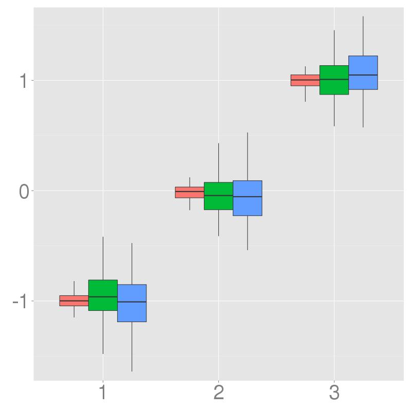
(a) Network effects

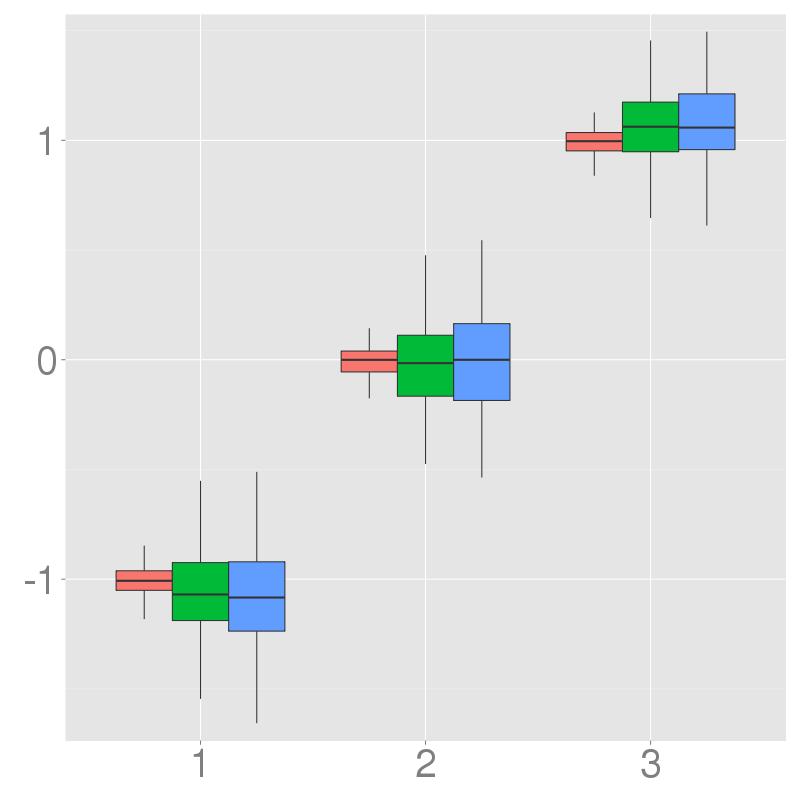
(b) Network effects with row normalization

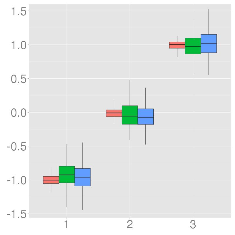
(c) Network disturbances

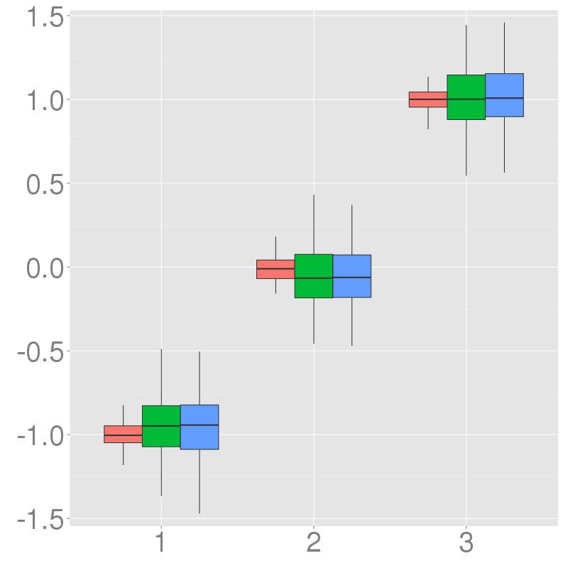
(d) Network disturbances with row normalization

Figure 2: Simulation study: Estimates for $\boldsymbol{\beta}$. True values are -1, 0 and 1. For each $\beta_{j}$, the boxplots correspond to, from left to right, the full data model, the proposed approach, and the OLS estimates ignoring network effects.

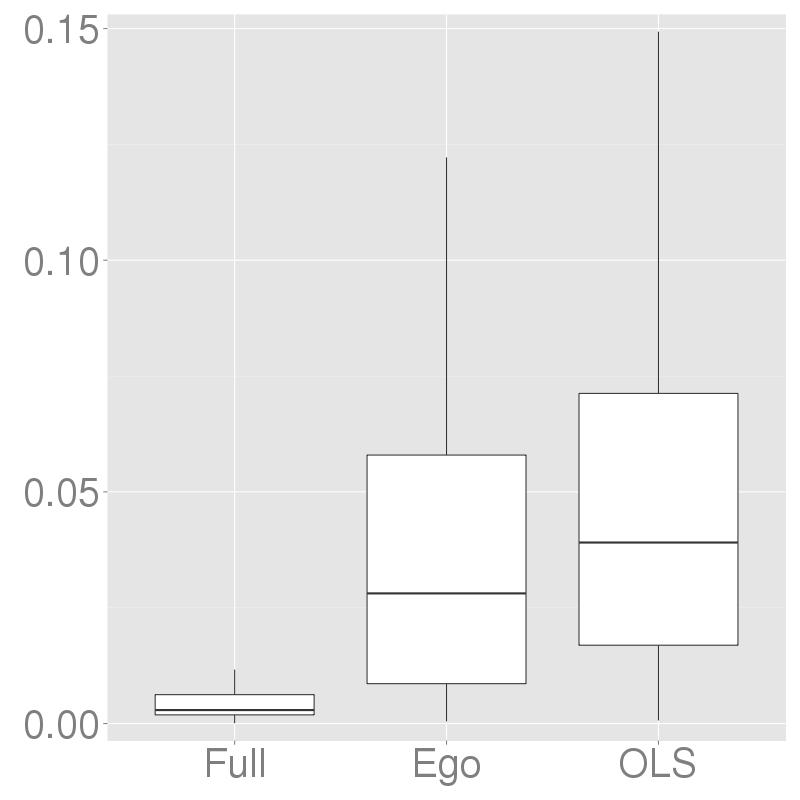
(a) Network effects

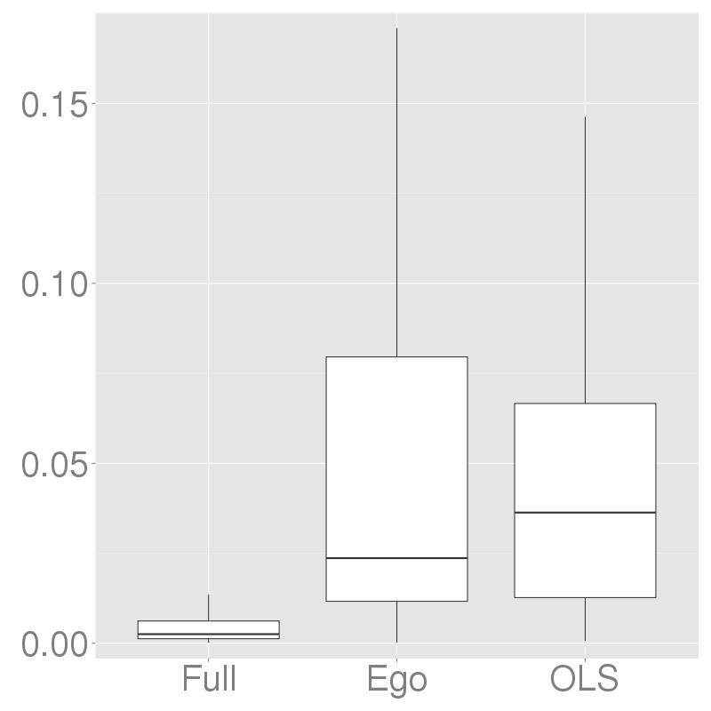
(b) Network effects with row normalization

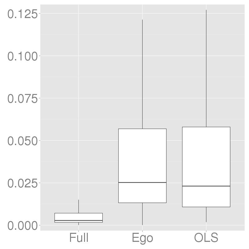
(c) Network disturbances

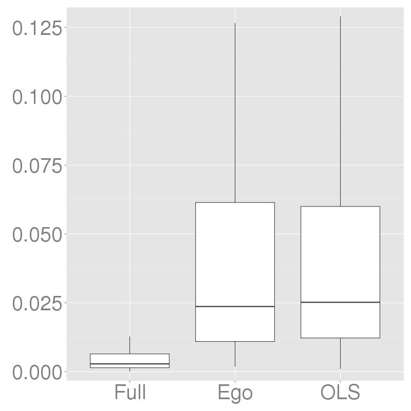
(d) Network disturbances with row normalization

Figure 3: Simulation study: MSE for $\boldsymbol{\beta}$ estimates.

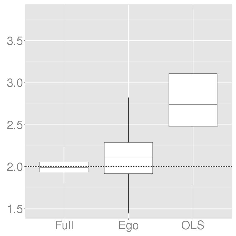
(a) Network effects

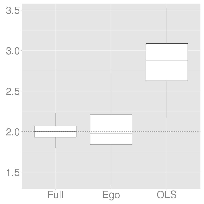
(b) Network effects with row normalization

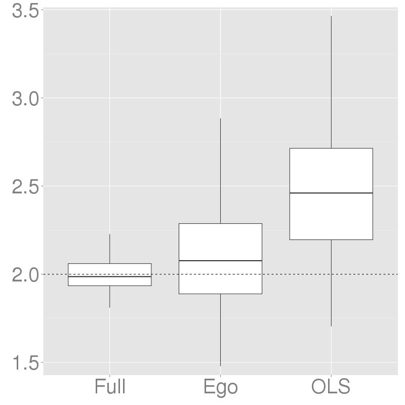
(c) Network disturbances

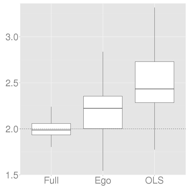
(d) Network disturbances with row normalization

Figure 4: Simulation study: Estimates for $\sigma^{2}$. True value is 2.

From Figure 5 we see that our proposed method seems to do a reasonable job of estimating the network effect, although there is, as alluded to earlier and seen in the literature for network autocorrelation models in general, a negative bias. This bias is much more severe in the models with row normalization. This is entirely unsurprising, as there is a considerable amount of additional uncertainty due to the unknown alter degrees. To a much lesser extent, there is also more bias exhibited in the network disturbances model compared with the network effects model. This too is unsurprising, because the network effects model inherently uses more information than the network disturbances model in estimating the influence not directly attributable to $\boldsymbol{y}_{e}$. That is, in the network effects model, the non-ego influence ($\rho A_{ea}\boldsymbol{y}_{a}$ in (4)) can in part be explained by the known alter covariate information $X_{a}$ and observed responses $\boldsymbol{y}_{e}$, whereas in the network disturbances model, the non-ego influence ($\rho A_{ea}(\boldsymbol{y}_{a}-X_{a}\boldsymbol{\beta})$ in (8)) is constructed from unknown residuals ($\boldsymbol{\nu}$ in (2)).

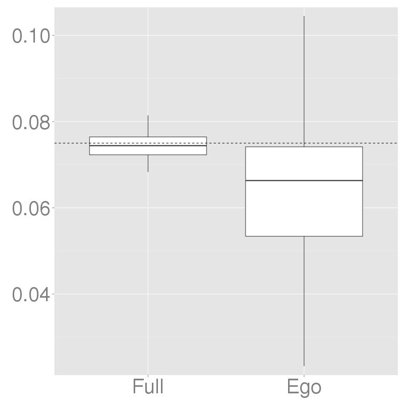
(a) Network effects

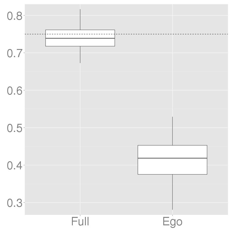
(b) Network effects with row normalization

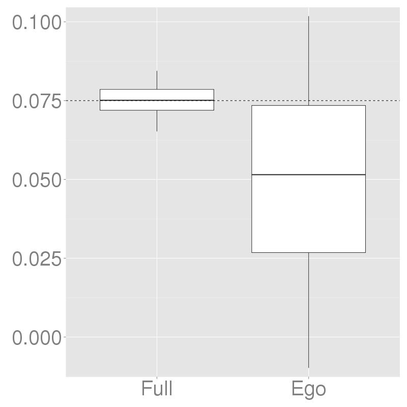
(c) Network disturbances

(d) Network disturbances with row normalization

Figure 5: Simulation study: Estimates for $\rho$. True value is 0.075, or .75 in the context of row normalization.

4 Environmental mastery in older adults

Researchers in the Department of Community and Behavioral Health at the University of Iowa collected a rich egocentric network data set on older adult subjects in a rural southeastern Iowa town (see, e.g., Ashida et al., 2016). One-time interviews were conducted with individuals in which a large number of attributes were collected as well as a variety of dyadic relationships corresponding to the ego. Here we make use of a subset of this dataset, focusing on an index that represents an individual’s environmental mastery. Specifically, the questions (given in Table 1) are taken from the Ryff scales of psychological well-being (Ryff & Keyes, 1995). This is an important aspect of the psychology of older adults, and we wish to investigate the notion that there is a network effect on older adults’ environmental mastery after accounting for some basic demographic information. Specifically, we control for gender, race (white or non-white), and age. The network under consideration was obtained by looking at, for each ego, all individuals with whom the ego sees at least once a week.

There are 119 egos in the data set and a total of 561 alters. Some of the egos nominated each other, and hence $A_{e}$ is not a matrix of 0’s. The density of $A_{e}$ and $A_{ea}$ were both 0.009 after rounding to three decimal places. The mean degree of the egos was 6.15, ranging from 1 to 18. Figure 6 shows the network.

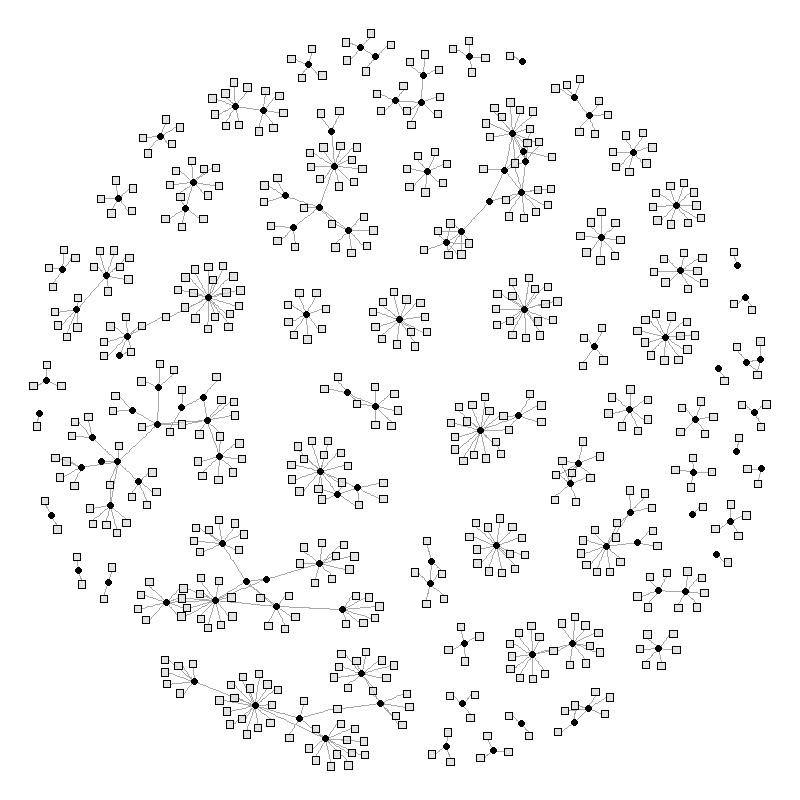
Figure 6: Environmental mastery egocentric network. Black circles are the observed egos. Gray squares are the alters.

We applied both the network effects and disturbances models both with and without row-normalization, running an MCMC algorithm with 300,000 iterations, using 50,000 of these as a burn-in. Table 2 gives the maximum log likelihood values for each of the four implemented models. Since the network effects model and the network disturbances model have the same number of parameters, and since those models with row normalization have even more parameters (due to estimating the degree distribution of the alters), both AIC and BIC would favor the network effects model without row normalization, and hence further inference is based on this.

Figure 7 gives the trace plots of the model parameters. These figures indicate very strongly that the MCMC algorithm converged. The posterior means and 90% credible regions for the model parameters are given in Table 3, and the histograms of the posterior samples for Female, Non-white, Age, and $\rho$ are given in Figure 8. From this we see that of the basic demographics, there is only evidence that age plays a non-trivial role in environmental mastery. We also see evidence in favor of a network effect. In fact, there is a 0.969 posterior probability that there is a positive network effect (i.e., $\mathbb{P}(\rho>0|\mbox{data})=0.969$). We may then conclude that an individual’s environmental mastery is affected by the environmental mastery with whom the individual is in contact on a regular basis. This type of conclusion may help shape future interventions by focusing on actors with high degree to maximize intervention impact.

Environmental Mastery Survey Questions
1. In general, I feel I am in charge of the situation in which I live.
2. The demands of everyday life often get me down.
3. I do not fit very well with the people and the community around me.
4. I am quite good at managing the many responsibilities of my daily life.
5. I often feel overwhelmed by my responsibilities.
6. I have difficulty arranging my life in a way that is satisfying to me.
7. I have been able to build a home and a lifestyle for myself that is much to my liking.

Table 1: List of Likert scale questions used to construct the environmental mastery scores. Questions 2, 3, 5, and 6 are reverse coded.

Model	Log-likelihood
Network effects without row normalization	-30.31
Network effects with row normalization	-33.81
Network disturbances without row normalization	-31.34
Network disturbances with row normalization	-35.65

Table 2: Environmental mastery data: Log-likelihood values for each of the four models implemented.

Parameter	Posterior mean (90% Credible Interval)
Intercept	27.4 (22.6,32.3)
Female	0.178 (-1.68,2.04)
Non-white	0.589 (-1.77,2.95)
Age	0.0850 (0.0185,0.152)
$\sigma^{2}$	32.6 (26.2,40.3)
$\rho$	0.00788 (0.000894,0.0153)

Table 3: Environmental mastery data: Posterior means and 90% credible intervals for the model parameters.

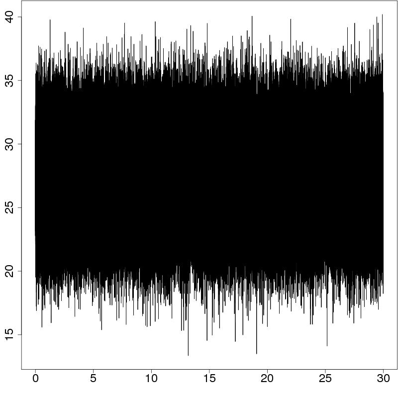
(a) Intercept

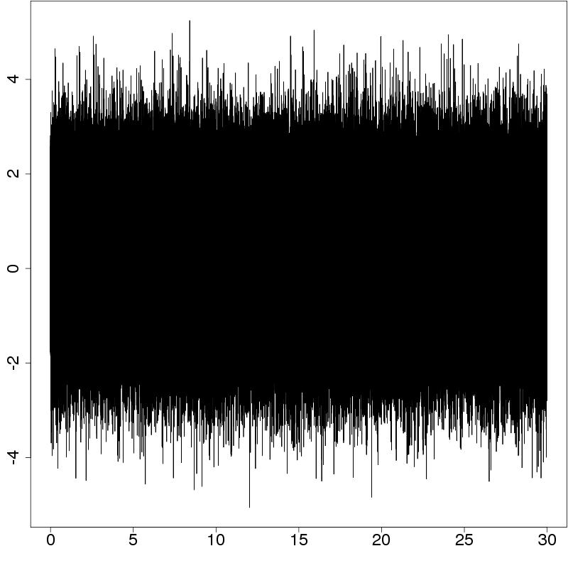
(b) Female

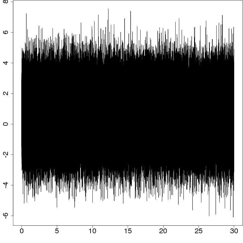
(c) Non-white

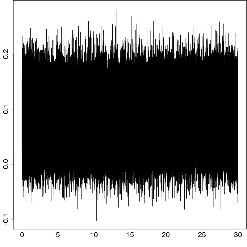
(d) Age

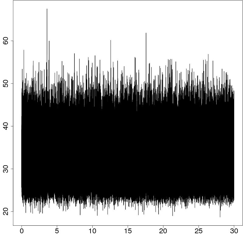
(e) $\sigma^{2}$

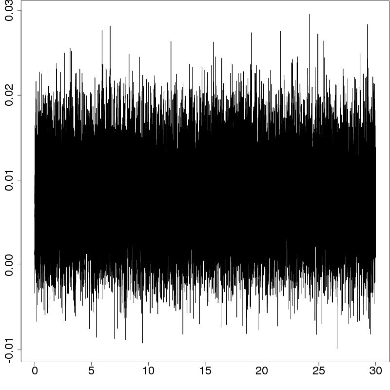
(f) $\rho$

Figure 7: Environmental mastery data: Trace plots of model parameters. The x-axis is in 10,000 iterations.

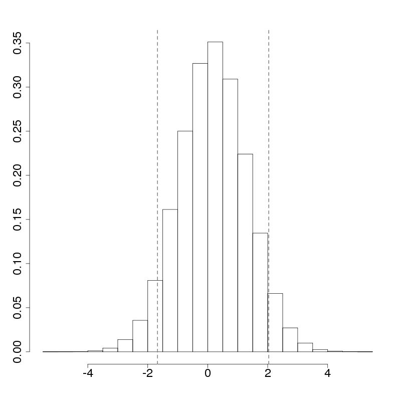
(a) Female

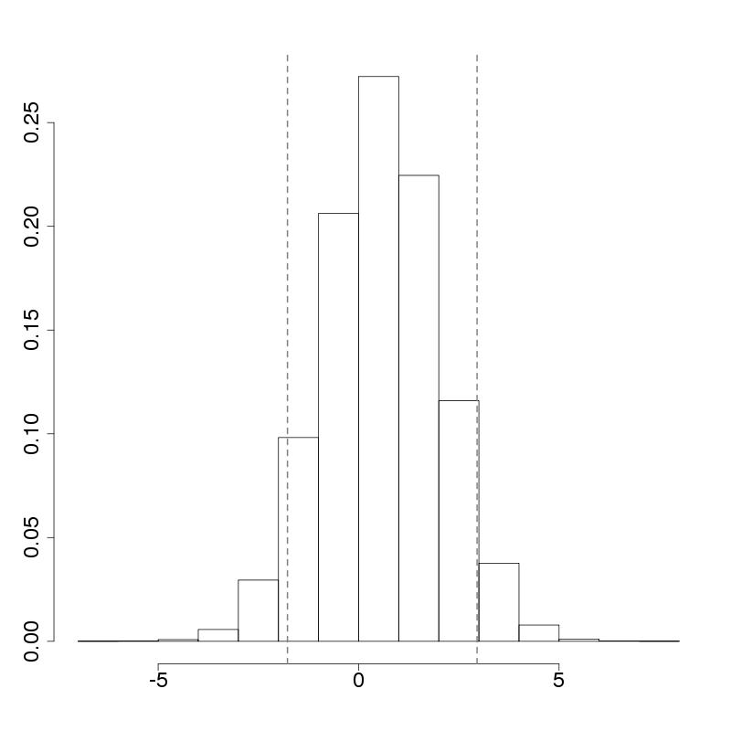
(b) Non-white

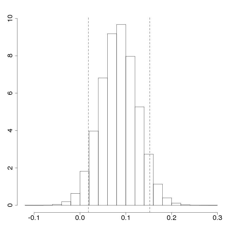
(c) Age

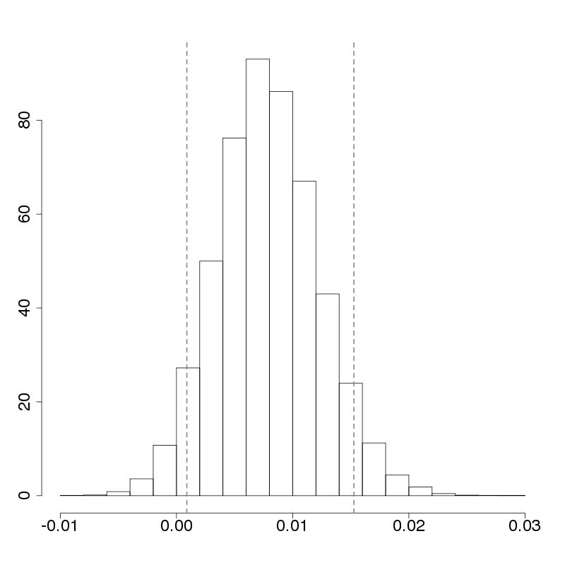
(d) $\rho$

Figure 8: Environmental mastery data: Histograms of the posterior samples for the mean coefficients for Female, Non-white, and Age, as well as the histogram for $\rho$. Vertical dotted lines represent the lower and upper bounds for the 90% credible region.

5 Discussion

Network autocorrelation models are widely used to measure covariate and network effects on a response variable of interest. These models, however, necessitate data on all actors of the network. This is very often not feasible. Egocentric network data are very often dramatically more feasible to collect, but the current methods to estimate network effects on this type of data are ad hoc, and not founded on a data generating process that could explain the full network data and all the complex dependencies therein.

This paper derives a model for egocentric data that is consistent with a data generating process that can account for the full network data. Specifically, if the true underlying generating process is a network autocorrelation model, the proposed conditional distribution used in this paper converges to the joint distribution of the data as $n_{e}\rightarrow n$. That is, when $n_{e}=n$, (7) is equivalent to the distribution of $\boldsymbol{y}$ as given in (1), and (12) is equivalent to the distribution of $\boldsymbol{y}$ as given in (3).

The negative bias in the estimation of the network effect as quantified by the parameter $\rho$ is an important issue in network autocorrelation models. The simulation study has shown that it is present in our context of egocentric data, and is especially problematic when there is row-normalization. It is the author’s hope that this is an area of future research that receives its due attention.

As mentioned earlier, a common ad hoc approach to estimating network effects with egocentric network data is to use as a covariate either network size or an average of some alter attribute. This can be viewed as using a spatial Durbin model, rather than a more sophisticated network autocorrelation model, only looking at a subset of the data. The Durbin model for the full data is

$$\boldsymbol{y}=X_{1}\boldsymbol{\beta}_{1}+AX_{2}\boldsymbol{\beta}_{2}+\boldsymbol{\epsilon},$$

where $X_{1}$ and $X_{2}$ may share some, all, or none of their columns. There is no complicated dependence structure in this model (which seems unrealistic in the network context), and so it is straightforward to use this model for egocentric data. Using the network size as a covariate is equivalent to letting $X_{2}$ be the vector of 1’s. Using the average of the alter attributes is equivalent to using a row-normalized $A$. Including lagged exogenous variables can be accounted for in the egocentric network autocorrelation models described in this paper, though some modification is necessary. Specifically, the network effects model becomes

$$\boldsymbol{y}_{e}|\boldsymbol{\alpha} \sim N\big{(}M_{1}^{-1}[(X_{1e}+\rho A_{ea}X_{1a})\boldsymbol{\beta}_{1}+((A_{e}+\rho A_{ea}A_{ea}^{\prime})X_{2e}+A_{ea}X_{2a})\boldsymbol{\beta}_{2}+\rho A_{ea}\boldsymbol{\alpha}],$$

$$\hskip 30.0pt\sigma^{2}M_{1}^{-1}M_{2}M_{1}^{-1}\big{)}$$ (20)

and similarly the network disturbances model becomes

$$\boldsymbol{y}_{e}|\boldsymbol{\alpha} \sim N\big{(}X_{1e}\boldsymbol{\beta}_{1}+(A_{e}X_{2e}+A_{ea}X_{2a})\boldsymbol{\beta}_{2}+\rho^{2}M_{1}^{-1}A_{ea}\boldsymbol{\alpha},\sigma^{2}M_{1}^{-1}M_{2}M_{1}^{-1}\big{)}.$$ (21)

Finally, recall that the network effects model leverages more information than the network disturbances model in explaining the non-ego influence, diminishing the ability to determine a network effect in the data. While this is obviously an important drawback of using the disturbances model rather than the network effects model, there is an important advantage here as well. Specifically, if it is not possible to measure the covariates on the alters, then while one may not implement the network effects model of (7) (at least not as given here), it is still possible to implement the network disturbances model of (12), as $X_{a}$ has no bearing on the network effect.

Appendix: Full conditional distributions

A1: Network effects model

The full conditional distribution for the variance $\sigma^{2}$ is given by

$$\sigma^{2}|\cdot \sim IG\left(\frac{a+n_{e}}{2},\frac{1}{2}\left[b+\|M_{2}^{-\frac{1}{2}}(M_{1}\boldsymbol{y}_{e}-(X_{e}+\rho A_{ea}X_{a})\boldsymbol{\beta}-\rho^{2}A_{ea}\boldsymbol{\alpha})\|^{2}\right]\right).$$

The full conditional distribution for the mean coefficients $\boldsymbol{\beta}$ is given by

$$\boldsymbol{\beta}|\cdot \sim N(\boldsymbol{\mu}_{b},\Sigma_{b}),$$

$$\boldsymbol{\mu}_{b} =\Sigma_{b}\left(\frac{1}{\sigma^{2}}(X_{e}+\rho A_{ea}X_{a})^{\prime}M_{2}^{-1}(M_{1}\boldsymbol{y}_{e}-\rho^{2}A_{ea}\boldsymbol{\alpha})+D^{-1}{\bf c}\right),$$

$$\Sigma_{b}^{-1} =\frac{1}{\sigma^{2}}(X_{e}+\rho A_{ea}X_{a})^{\prime}M_{2}^{-1}(X_{e}+\rho A_{ea}X_{a})+D^{-1}.$$

The full conditional distribution for the residual influence effects $\boldsymbol{\alpha}$ is given by

$$\boldsymbol{\alpha}|\cdot \sim N(\boldsymbol{\mu}_{a},\Sigma_{a})$$

$$\boldsymbol{\mu}_{a} =\Sigma_{a}\left(\frac{\rho^{2}}{\sigma^{2}}A_{ea}^{\prime}M_{2}^{-1}(M_{1}\boldsymbol{y}_{e}-(X_{e}+\rho A_{ea}X_{a})\boldsymbol{\beta})+F^{-1}{\bf e}\right),$$

$$\Sigma_{a}^{-1} =\frac{\rho^{4}}{\sigma^{2}}A_{ea}^{\prime}M_{2}^{-1}A_{ea}+F^{-1}.$$

A2: Network disturbances model

The full distribution for the variance $\sigma^{2}$ is given by

$$\sigma^{2}|\cdot \sim IG\left(\frac{a+n_{e}}{2},\frac{1}{2}\left[b+\|M_{2}^{-\frac{1}{2}}(M_{1}\boldsymbol{y}_{e}-M_{1}X_{e}\boldsymbol{\beta}-\rho^{2}A_{ea}\boldsymbol{\alpha})\|^{2}\right]\right).$$

The full conditional distribution for the mean coefficients $\boldsymbol{\beta}$ is given by

$$\boldsymbol{\beta}|\cdot \sim N(\boldsymbol{\mu}_{b},\Sigma_{b}),$$

$$\boldsymbol{\mu}_{b} =\Sigma_{b}\left(\frac{1}{\sigma^{2}}X_{e}^{\prime}M_{1}^{\prime}M_{2}^{-1}(M_{1}\boldsymbol{y}_{e}-\rho^{2}A_{ea}\boldsymbol{\alpha})+D^{-1}{\bf c}\right),$$

$$\Sigma_{b}^{-1} =\frac{1}{\sigma^{2}}X_{e}^{\prime}M_{1}^{\prime}M_{2}^{-1}M_{1}X_{e}+D^{-1}.$$

The full conditional distribution for the residual influence effects $\boldsymbol{\alpha}$ is given by

$$\boldsymbol{\alpha}|\cdot \sim N(\boldsymbol{\mu}_{a},\Sigma_{a})$$

$$\boldsymbol{\mu}_{a} =\Sigma_{a}\left(\frac{\rho^{2}}{\sigma^{2}}A_{ea}^{\prime}M_{2}^{-1}(M_{1}\boldsymbol{y}_{e}-M_{1}X_{e}\boldsymbol{\beta})+F^{-1}{\bf e}\right),$$

$$\Sigma_{a}^{-1} =\frac{\rho^{4}}{\sigma^{2}}A_{ea}^{\prime}M_{2}^{-1}A_{ea}+F^{-1}.$$

References

- (1)
- Ahuja (2000) G. Ahuja (2000). ‘Collaboration networks, structural holes, and innovation: A longitudinal study’. Administrative Science Quarterly 45(3):425–455.
- Anselin (1988) L. Anselin (1988). Spatial Econometrics: Methods and Models. Kluwer Academic Publishers.
- Ashida et al. (2016) S. Ashida, et al. (2016). ‘Reaching social network members of rural older adults: Who can we access and who would participate in social assessment?’. Unpublished .
- Ashida et al. (2009) S. Ashida, et al. (2009). ‘Changes in female support network systems and adaptation after breast cancer diagnosis: differences between older and younger patients’. The Gerontologist 49(4):549–559.
- Behrman et al. (2003) J. Behrman, et al. (2003). ‘Social networks, HIV/AIDS and risk perceptions’. IDEAS Working Paper Series from RePEc .
- Björklund (1990) M. Björklund (1990). ‘A phylogenetic interpretation of sexual dimorphism in body size and ornament in relation to mating system in birds’. Journal of Evolutionary Biology 3(3-4):171–183.
- Carpenter et al. (1998) D. P. Carpenter, et al. (1998). ‘The Strength of weak ties in lobbying networks: Evidence from health-care politics in the United States’. Journal of Theoretical Politics 10(4):417–444.
- Carr & Zube (2015) C. T. Carr & P. Zube (2015). ‘Network autocorrelation of task performance via informal communication within a virtual world’. Journal of Media Psychology: Theories, Methods, and Applications 27(1):33–44.
- Chun et al. (2012) Y. Chun, et al. (2012). ‘Modeling interregional commodity flows with incorporating network autocorrelation in spatial interaction models: An application of the US interstate commodity flows’. Computers, Environment and Urban Systems 36(6):583–591.
- Doreian (1980) P. Doreian (1980). ‘Linear models with spatially distributed data: Spatial disturbances or spatial effects?’. Sociological Methods and Research 9(1):29–60.
- Doreian (1989) P. Doreian (1989). ‘Network autocorrelation models: Problems and prospects’. Prepared for the 1989 Symposium “Spatial Statistics: Past, present, future,” Department of Geography, Syracuse University.
- Dow et al. (1982) M. M. Dow, et al. (1982). ‘Network autocorrelation: a simulation study of a foundational problem in regression and survey research’. Social Networks 4(2):169–200.
- Duke (1991) J. B. Duke (1991). ‘The peer context and the adolescent society: making sense of the context effects paradox’. PhD Thesis.
- Fisher (2005) D. Fisher (2005). ‘Using egocentric networks to understand communication’. IEEE Internet Computing 9(5):20–28.
- Fujimoto et al. (2011) K. Fujimoto, et al. (2011). ‘The network autocorrelation model using two-mode data: Affiliation exposure and potential bias in the autocorrelation parameter’. Social Networks 33(3):231–243.
- Granovetter (1976) M. Granovetter (1976). ‘Network sampling: Some first steps’. American Journal of Sociology 81(5):1287–1303.
- Heckathorn (1997) D. D. Heckathorn (1997). ‘Respondent-driven sampling: A new approach to the study of hidden populations’. Social Problems 44(2):174–199.
- Leenders (2002) R. T. A. J. Leenders (2002). ‘Modeling social influence through network autocorrelation: Constructing the weight matrix’. Social Networks 24(1):21–47.
- Mizruchi & Neuman (2008) M. S. Mizruchi & E. J. Neuman (2008). ‘The effect of density on the level of bias in the network autocorrelation model’. Social Networks 30(3):190–200.
- O’Malley et al. (2012) A. J. O’Malley, et al. (2012). ‘Egocentric social network structure, health, and pro-social behaviors in a national panel study of Americans’. PLOS One 7(5):e36250.
- Ord (1975) K. Ord (1975). ‘Estimation methods for models of spatial interaction’. Journal of the American Statistical Association 70(349):120–126.
- Provan et al. (2007) K. G. Provan, et al. (2007). ‘Interorganizational networks at the network level: A review of the empirical literature on whole networks’. Journal of Management 33(3):479–516.
- Ryff & Keyes (1995) C. D. Ryff & C. L. M. Keyes (1995). ‘The structure of psychological well-being revisited’. Journal of Personality and Social Psychology 69(4):719–727.
- Smith (2004) T. E. Smith (2004). Spatial Econometrics and Spatial Statistics. Macmillan, New York.
- Wang et al. (2014) W. Wang, et al. (2014). ‘Statistical power of the social network autocorrelation model’. Social Networks 38:88–99.
- White et al. (1981) D. R. White, et al. (1981). ‘Sexual division of labor in African agriculture: A network autocorrelation analysis’. American Anthropologist 83(4):824–849.