Quantum-Classical Machine learning by Hybrid Tensor Networks

Abstract

Tensor networks (TN) have found a wide use in machine learning, and in particular, TN and deep learning bear striking similarities. In this work, we propose the quantum-classical hybrid tensor networks (HTN) which combine tensor networks with classical neural networks in a uniform deep learning framework to overcome the limitations of regular tensor networks in machine learning. We first analyze the limitations of regular tensor networks in the applications of machine learning involving the representation power and architecture scalability. We conclude that in fact the regular tensor networks are not competent to be the basic building blocks of deep learning. Then, we discuss the performance of HTN which overcome all the deficiency of regular tensor networks for machine learning. In this sense, we are able to train HTN in the deep learning way which is the standard combination of algorithms such as Back Propagation and Stochastic Gradient Descent. We finally provide two applicable cases to show the potential applications of HTN, including quantum states classification and quantum-classical autoencoder. These cases also demonstrate the great potentiality to design various HTN in deep learning way.

I Introduction.

In recent year, tensor networks (TN) have drawn more attention as one of the most powerful numerical tools for studying quantum many-body systems (Verstraete et al., 2008a; Orús, 2014a, b; Ran et al., 2017). Furthermore, TN have been recently applied to many research areas of machine learning  (Orús, 2019; Efthymiou et al., 2019; Roberts et al., 2019; Sun et al., 2020), such as image classification  (Stoudenmire and Schwab, 2016; Han et al., 2017; Liu et al., 2019), dimensionality reduction (Cichocki et al., 2016, 2017), generative model (Cheng et al., 2019; Han et al., 2017), data compression (Li and Zhang, 2018), improving deep neural network (Kossaifi et al., 2017), probabilistic graph model (Ran, 2019a), quantum compressed sensing (Ran et al., 2019), even the promising way to implement quantum circuit (Huggins et al., 2018; Benedetti et al., 2018; Bhatia et al., 2019; Ran, 2019b; Wang et al., 2020). As a consequence, people encounter the serious computing complexity problem and raise the question: Are the tensor networks able to be the universal deep learning architecture? As we know, the theoretical foundation of deep neural networks is the principle of universal approximation which states that a feed-forward network with a single hidden layer is a universal approximator if and only if the activation function is not polynomial  (Leshno et al., 1993; Hornik, 1991). In this context, the key point of the question of tensor network machine learning will be: Are the tensor networks able to be the universal approximator?

Some pioneering researches have started to focus on this fundamental problem. Ref. Glasser et al. (2018) propose the concept of generalized tensor networks to outperform the regular tensor networks particularly in term of the representation power. Specifically, if the entanglement entropy of the function violates the area low (Verstraete et al., 2008b), then the function can not be represented by regular tensor networks efficiently. Moreover, they try to combine generalized tensor networks with convolution neural networks together and achieve some good results. Note that they take the convolutions as feature map, then place tensor network in the final layer and take it as the classifier. Ref. (Kossaifi et al., 2017) propose the tensor regression network which replace the full connect layer by tensor regression layer in order to save storage space.This is another feasible way to take advantage of tensor network in deep learning. Ref. (Glasser et al., 2019) provides a mathematic analysis of the representation power of some typical tensor network factorizations of discrete multivariate probability distributions involving matrix product states (MPS), Born machines and locally purified states (LPS). Ref. (Chen et al., 2018) discusses the equivalence of restricted boltzmann machines (RBM) and tensor network states. They prove that this kinds of specific neural networks can be translated into MPS and devise efficient algorithm to implement it. And based on this, they quantify the representation power of RBM from the perspective of tensor network. This insight into tensor network and RBM guides the design of novel quantum deep learning architectures.

Different from these previous works, we propose the concept of Hybrid Tensor Networks (HTN) which combine tensor networks with classical neural networks into a uniform deep learning framework. We show the schematic of this universal framework of HTN in Fig. 1. In this framework, people are able to freely design HTN by adding some specific tensor networks such as Matrix Product States (MPS), Projected Entangled Pair States (PEPS) or Tree Tensor Networks (TTN) etc., and some classical neural networks such as Fully-connected Networks (FCN), Convolutional Neural Networks (CNN) or Recurrent Neural Networks (RNN) etc. at any part of the HTN. And then train the whole network by the standard combination of training algorithms such as the Back Propagation (BP) and Stochastic Gradient Descent (SGD). Therefore by introducing neuron with nonlinear activation, HTN will be the universal approximator as same as neural network. More importantly, HTN are capable of dealing with quantum input states involving both quantum entanglement states and product states. In this way, the HTN will be a good choice of the implementation of quantum-classical deep learning model. Specifically, we discuss some preliminary ideas to design HTN and provide some applicable cases and numerical experiments.

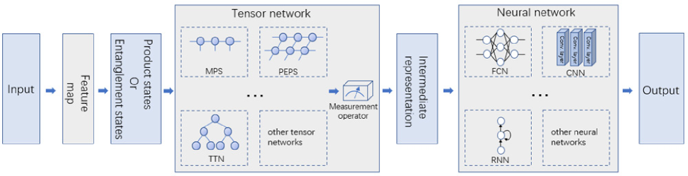
Figure 1: Universal framework of Hybrid Tensor Networks.

II Limitations of regular tensor networks machine learning

Although, as a kind of popular and powerful numerical tools in quantum many-body physics, regular tensor networks expose some limitations on machine learning, such as the limitations on representation power and architecture scalability. All of these limitations restrict the application of regular tensor networks on machine learning, especially for deep learning. In this section, we conclude it and also analyze some main points of them.

II.1 Representation power

General neural networks (NNs) are characterized by the universal approximation theorem which states that the feed-forward networks are able to approximate any continuous function, which owing to the use of nonlinear activation. So we treat it as a kind of so called universal approximator. Based on this, NNs become the fundamental building blocks of deep learning. In contrast, TNs are considered as linear function and therefore obey the superposition principle in quantum mechanics. This is characterized as the intrinsic feature of TNs in quantum many-body system, but an obstacle to be a powerful universal approximator in machine learning. In this context, people have to map all data points from original feature space into the higher Hilbert space by means of nonlinear feature map function. In some previous works (Liu et al., 2019; Stoudenmire and Schwab, 2016), people use the feature map which is introduced by Eq.1 firstly as:

$$v_{s}(x)=\sqrt{\binom{d-1}{s-1}}(\cos(\frac{\pi}{2}x))^{d-{s}}(\sin(\frac{\pi}{2}x))^{s-1}$$ (1)

where $s$ runs from $1$ to $d$. By using a larger $d$, the TTN has the potential to approximate a richer class of functions. Furthermore, Ref.Glasser et al. (2018) discuss some other complex feature maps we could use, even including neural networks such as CNNs. Based on these works, we understand that the feature map actually play the key role in tensor network machine learning, since it makes the model with the capacity of approximating nonlinear function. It is also easy to understand this from the perspective of statistical machine learning theory such as Support Vector Machine (SVM). In the context of SVM, people always map data points into a higher feature space and find a kernel function while addressing the nonlinear issue, and it is called the “kernel trick”. However, in the context of tensor network machine learning, we shouldn’t just rely on this “kernel trick” to endow the TNs with the capacity of universal approximation while building a complex and deep tensor network model.

Moreover, for a specific machine learning task, we always have to train a bigger regular tensor network which contains much more parameters than corresponding classical neural network. Taking our previous work as example (Liu et al., 2019), we employed the TTN on benchmark of handwritten digits classification. The experimental results show us TTN contains too much parameters than almost any classical model such as CNN and fully-connected network (FCN). For comparison, we also implement a HTN model and find the number of parameters it needs is less than FCN’s, of course far less than TTN’s. We conclude all these results in the Table 1. From the perspective of quantum simulation, we understand that simulating quantum computing on classical computer always needs exponential growth of parameters with the size of systems. It shows us the large number of parameters intrinsically leads to a severe problem -–- comparing with existing deep learning model, it is difficult to train a regular tensor network which has a same or better performance, even it is impossible.

We also verify this conclusion by using some preliminary regression experiments which directly reveal the model’s capability of curve fitting. Table 2 shows us the benchmark results on MNIST dataset. In this case, we transfer the classification task into a simple regression issue by setting the label as a corresponding scalar. Taking the class of image “6” as the example, we need to train a model that outputs a scalar which closes to “6” as soon as possible, rather than a classification vector. We then determine the lower bound of the Mean Square Error loss function (MSE) and find the minimum model which could reaches this lower bound. Indeed, the lower bound of loss function characterizes the upper bound of the model’s capability of curve fitting. Clearly, the TTN contains much more parameters than FCN and CNN to reach the same level of lower bonds. In this case, it has $10^{2}$ or $10^{3}$ times larger than that of the FCN or CNN. It will lead to severe time consuming problem and even in some worst cases, the training likely to fail. Similar with the last case, we also find the number of parameters HTN needs is less than FCN’s, and far less than TTN’s.

II.2 Architecture scalability

We also evaluate regular tensor network machine learning from the perspective of architecture scalability. As we know, people develop a great many of deep learning models to meet the challenges in computer vision, natural language processing and speech recognition etc., such as the popular CNN (LeCun et al., 1995), RNN, LSTM (Hochreiter and Schmidhuber, 1997), GAN (Goodfellow et al., 2014), Attention model and Transformer (Vaswani et al., 2017) etc. So just like playing Jenga game, people are always able to assemble all these models together depending on the engineering applications in practice, even for the designing of extremely deep and complex architecture. In contrast, people have to strictly restrict the scale of tensor networks while applying them into quantum many-body systems or machine learning, since the rapid growth of computational complexity. Ref. (Orús, 2019) concludes some popular tensor networks such as MPS, PEPS, TTN and MERA. So far, to our knowledge, just MPS, MERA and TTN are employed in the preliminary applications of machine learning.

Apart from it, we take the process of message passing into consideration and find the significant different behaviour between the tensor networks and neural networks. As we show in Fig.2, the message passes through a neural network from the input side to the output end layer by layer. Specifically, for any single neuron in any layer, the input message could be distributed into multi output directions, and then access to the next layer. In a formal style, we denote the out-degree of a single neuron as $D_{out}$ and the in-degree as $D_{in}$. Then as we know, in a neural network, any neuron is capable of having much larger $D_{out}$ than $D_{in}$, such as fully-connected network . This guarantees the one-to-many mapping could be implemented easily by neural networks. In contrast, Fig.2 and Fig.2 show us the process of message passing in two typical tensor networks including MPS and TTN. Since the message passing is implemented by the operation of tensor contraction, thus for a single unit/local tensor, the input message can’t be distributed into multi output directions like what neural network can do, unless the operation of tensor decomposition is involved. This mechanism definitely limits the scalability of regular tensor networks in machine learning, especially in the case that we need to build a deep hierarchy.

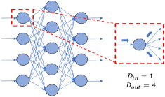
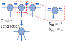
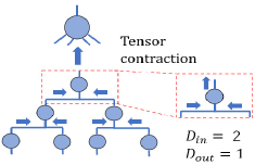
Figure 2: Different ways of message passing on Neural Networks and Tensor Networks. The directions of message passing are denoted by blue arrows. For tensor network, the message passing is implemented by the operation of tensor contraction; (a) Neural Network ; (b) MPS; (c) TTN;

Based on all these observations, we understand the lack of architecture scalability is another severe problem for regular tensor network machine learning. For all these reasons, we think it’s not the good way to build a huge, deep and complex deep learning model by regular tensor networks for the practical applications of machine learning. Therefore, how can we take the advantages of tensor networks for deep learning? The solution we try to offer is the Hybrid Tensor Network.

Table 1: Number of parameters of each model on MNIST classification

model	TTN	LeNet-5	FCN	HTN
Test accuracy	95%	99%	95%	98%
Number of
parameters	$1.4\times 10^{9}$	$1.2\times 10^{4}$	$2.4\times 10^{6}$	$7.7\times 10^{5}$

Table 2: Number of parameters of each model on MNIST regression

MSE Loss	$O(10^{-1})$	$O(10^{-2})$
FCN	$8.6\times 10^{3}$	$6\times 10^{4}$
CNN	$6\times 10^{2}$	$3\times 10^{3}$
TTN	$4.3\times 10^{4}$	$1.4\times 10^{6}$
HTN	$6.5\times 10^{3}$	$2.6\times 10^{4}$

III Hybrid Tensor Networks

We propose the concept of Hybrid Tensor Networks (HTN) to overcome the limitations on both representation power and scalability of regular tensor network in machine learning. The basic idea is to introduce the nonlinearity by the combination of tensor networks and neural networks. In this way, we are able to embed a tensor network into any existing popular deep learning framework very easily, involving both model and algorithm such as CNN, RNN, LSTM etc.. Then we are able to train a HTN by the standard Back Propagation algorithm (BP) and Stochastic Gradient Descend (SGD) which can be easily found at any deep learning literature (Goodfellow et al., 2016). Suppose we have a HTN which formed in the sequence of $n$ tensor network layers $T_{1},T_{2},...,T_{n}$, and subsequent $m$ neural network layers $L_{1},L_{2},...,L_{m}$. The cost function is denoted as $Cost$. Then we could compute the partial derivative to the $ith$ tensor network layer owing to the BP algorithm by Eq. 2.

$${\frac{{\partial Cost}}{{\partial\mathop{{T}}\nolimits_{{i}}}}=\frac{{\partial Cost}}{{\partial\mathop{{L}}\nolimits_{{m}}}}⸳{\frac{{\partial\mathop{{L}}\nolimits_{{m}}}}{{\partial\mathop{{L}}\nolimits_{{m-1}}}}...{\frac{{\partial\mathop{{L}}\nolimits_{{1}}}}{{\partial\mathop{{T}}\nolimits_{{n}}}}⸳{\frac{{\partial\mathop{{T}}\nolimits_{{n}}}}{{\partial\mathop{{T}}\nolimits_{{n-1}}}}...\frac{{\partial\mathop{{T}}\nolimits_{{i+1}}}}{{\partial\mathop{{T}}\nolimits_{{i}}}}}}}}$$ (2)

Since the operation of tensor contraction defined as Eq. 3 is doubtless differentiable,

$${T\mathop{{}}\nolimits_{{i+1}}^{{\left[k\right]}}={\mathop{\sum}\limits_{{\mathop{{\alpha}}\nolimits_{{1}}...\mathop{{\alpha}}\nolimits_{{p}}}}{\mathop{{T}}\nolimits_{{i,\mathop{{\alpha}}\nolimits_{{1}}}}^{{\left[1\right]}}\mathop{{T}}\nolimits_{{i,\mathop{{\alpha}}\nolimits_{{2}}}}^{{\left[2\right]}}...\mathop{{T}}\nolimits_{{i,\mathop{{\alpha}}\nolimits_{{p}}}}^{{\left[p\right]}}}}}$$ (3)

where $T_{i+1}^{[k]}$ represents the $kth$ tensor in the $i+1$ layer. So the last term of Eq. 2 can be deduced as Eq. 4,

$$\begin{aligned} \frac{{\partial\mathop{{T}}\nolimits^{{\left[k\right]}}_{{i+1}}}}{{\partial\mathop{{T}}\nolimits_{{i}}\mathop{{}}\nolimits^{{\left[j\right]}}}}&=\frac{{{\partial\mathop{\sum}\limits_{{\mathop{{\alpha}}\nolimits_{{1}}...\mathop{{\alpha}}\nolimits_{{p}}}}{\mathop{{T}}\nolimits^{{\left[1\right]}}_{{i,\mathop{{\alpha}}\nolimits_{{1}}}}...\mathop{{T}}\nolimits^{{\left[j\right]}}_{{i,\mathop{{\alpha}}\nolimits_{{j}}}}...\mathop{{T}}\nolimits^{{\left[p\right]}}_{{i,\mathop{{\alpha}}\nolimits_{{p}}}}}}}}{{\partial\mathop{{T}}\nolimits_{{i}}\mathop{{}}\nolimits^{{\left[j\right]}}}}\\ &={\mathop{\sum}\limits_{{\mathop{\alpha}\nolimits_{{1}}...\mathop{{\alpha}}\nolimits_{p}}\}\backslash\{\mathop{{\alpha}}\nolimits_{{j}}\}}{\mathop{{T}}\nolimits^{{\left[1\right]}}_{{i,\mathop{{\alpha}}\nolimits_{1}}}...\mathop{T}\nolimits^{{\left[j-1\right]}}_{{i,\mathop{{\alpha}}\nolimits_{j-1}}}\mathop{T}\nolimits^{{\left[j+1\right]}}_{{i,\mathop{{\alpha}}\nolimits_{j+1}}}...\mathop{{T}}\nolimits^{{\left[p\right]}}_{{i,\mathop{{\alpha}}\nolimits_{p}}}}}\end{aligned}$$ (4)

where $T_{i}^{[j]}$ represents the $jth$ tensor in the $ith$ layer. And the rest terms of Eq. 2 could be calculated easily according to the principle of neural networks. Then, we can update this tensor by using gradient descend method as Eq. 5,

$${\mathop{{T}}\nolimits_{{i}}^{{{}^{\prime}}}=\mathop{{T}}\nolimits_{{i}}-\eta\frac{{\partial Cost}}{{\partial\mathop{{T}}\nolimits_{{i}}}}}$$ (5)

where $\eta$ denotes the learning rate. Indeed all tensors in HTN could be updated layer by layer following this way. Therefore, it guarantees that the HTN can be trained in the uniform optimization framework which combines BP and SGD. Some popular deep learning open-source software library such as Tensorflow (Abadi et al., 2016) and Pytorch (Paszke et al., 2017) offer powerful automatic differentiation program libraries which could help us implement HTN very easily.

Furthermore, we speed up the basic operation of tensor contraction on GPU platform, which is shown in Fig. 3. It confirms the feasibility of implementing HTN model by utilizing GPU platform, and shed light on the potential, complex and practical applications of large scale HTN model in the real-world.

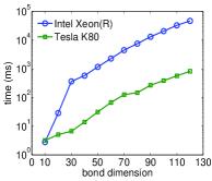
Figure 3: Speeding up on triangle tensor network contraction by GPU platform. The time cost is plotted on logarithmic y-axis.

It should be noted, different from previous work that combines tensor networks and neural networks Glasser et al. (2018), we treat tensor networks as the “quantum units” which is in charge of extracting quantum features from input states. So for the designing of a deep HTN, the first thing we should consider is to understand exactly the role tensor networks will play. We show our two preliminary attempts on quantum states classification and quantum-classical autoencoder in the following.

III.1 Quantum states classification

We design a simple HTN architecture with two tree tensor network layers followed by three dense neural network layers to verify the practicability of it in classification problem. In this case, we first transform the input images into quantum product states without entanglement, which is formed as Eq.6,

$$\left|\Phi\right\rangle={\left|{\phi{\left({x\mathop{{}}\nolimits_{{1}}}\right)}}\right\rangle}\otimes{\left|{\phi{\left({x\mathop{{}}\nolimits_{{2}}}\right)}}\right\rangle}...\otimes⸳{\left|{\phi{\left({x\mathop{{}}\nolimits_{{n}}}\right)}}\right\rangle}$$ (6)

where $x_{1},x_{2},...,x_{n}$ represents each pixel; $\left|\Phi\right\rangle$ is the product states we get in the high dimensional Hilbert space; $\phi$ denotes the feature map we mentioned by Eq.1. We define the tree tensor network as $\left|\Psi\right\rangle$, so these two tree tensor network layers encode the $\left|\Phi\right\rangle$ into the intermediate low dimensional states $\left|I\right\rangle$ by tensor contraction, i.e. ${{\left|{I}\right\rangle}={\left\langle{\Psi}\left|{\Phi}\right\rangle\right.}}$. Afterwords, this intermediate states could be readout by $c={\left\langle{I}\right|}M{\left|{I}\right\rangle}$, where $M$ is the measurement operator and the $c$ denotes the classical data that could be processed by neural networks. For simplicity, we merge measurement into tensor network by letting the dimension of output bonds equal to one.

Finally, the subsequent dense neural network layers classify the intermediate $c$ into 10 corresponding categories by using cross entropy cost function and the popular Adam training algorithm (Kingma and Ba, 2014) which derived from the standard SGD. The cross entropy is defined as Eq.7

$$CroEn{\left({L,P}\right)}=-{\mathop{\sum}\limits_{{i=1}}^{{n}}{L\left(c\mathop{{}}\nolimits_{{i}}\left)log\left(P\left(c\mathop{{}}\nolimits_{{i}}\left)\right)\right.\right.\right.\right.}}$$ (7)

where $L$ refers to the label and $P$ is the predicted output by HTN. As can be seen, in analogy with the classical CNNs, the tensor network layers play the similar role with the convolutional layers. But different from it, tensor networks are more applicable to quantum states processing. We use the popular MNIST and Fashion-MNIST datasets as the benchmarks. The training set consists of 60 000 ($28\times 28$) gray-scale images, with 10 000 testing examples. For the simplicity of coding, we rescaled them to (32$\times$32) images by padding zeros pixels. We show the schematic in Fig.4. It is easy to get 98% test accuracy on MNIST and 90% test accuracy on Fashion-MNIST benchmarks by using this simple HTN architecture without using any deep learning tricks.

The overview of experimental results of numerous classical models on these tasks could be found at the official website: (http://yann.lecun.com/exdb/mnist/) and (https://github.com/zalandoresearch/fashion-mnist). Though our method applies to the complex HTN, we assume all tensors are real for simplicity. Our code of the implementation is available at , and people could find the setup of parameters in detail from it.

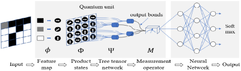
Figure 4: HTN for quantum states classification. We embed two tree tensor network layers and three dense neural network layers.

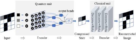
Figure 5: HTN for Quantum-classical autoencoder. We create the encoder by two tensor network layers, and design three different decoders by using three different setups of deconvolutional layers.

III.2 Quantum-Classical Autoencoder

We then show the application of quantum autoencoder by using a variety of HTNs. For simplicity, we still benchmark all models on MNIST and Fashion-MNIST datasets. In this case, the encoder formed by a tensor network which compresses the input quantum states into low dimensional intermediate states. Next, these compressed intermediate states could be recovered by some typical classical neural networks. We continue to use the Adam training algorithm, but change the cost function as MSE (Mean Square Error):

$$MSE=\frac{{1}}{{n}}{\mathop{\sum}\limits_{{i=1}}^{{n}}{\left(I\mathop{{}}\nolimits_{{i}}-O\mathop{{}}\nolimits_{{i}}\left)\mathop{{}}\nolimits^{{2}}\right.\right.}}$$ (8)

where $I$ is input data, and $O$ denotes the reconstructed data. Fig.5 shows us the basic architecture and we can find the detailed setup of parameters in our code which is available at .

We show a series of experimental results in both Fig.6 and Fig.7, and provide the evaluation indicators Compression Ratio (CR) and PSNR (Peak Signal-to-Noise Ratio) which is defined as Eq.9:

$$PSNR=10*log\mathop{{}}\nolimits_{{10}}\left(\frac{{max\mathop{{}}\nolimits_{{I}}^{{2}}}}{{\frac{{1}}{{mn}}{\mathop{\sum}\limits_{{i=1}}^{{m}}{{\mathop{\sum}\limits_{{j=1}}^{{n}}{\left(O\mathop{{}}\nolimits_{{i,j}}-P\mathop{{}}\nolimits_{{i,j}}\left)\mathop{{}}\nolimits^{{2}}\right.\right.}}}}}}\right)$$ (9)

where $max_{I}$ indicates the max value of input data.

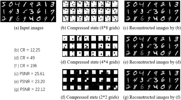
Figure 6: Quantum-Classical Autoencoder on MNIST;

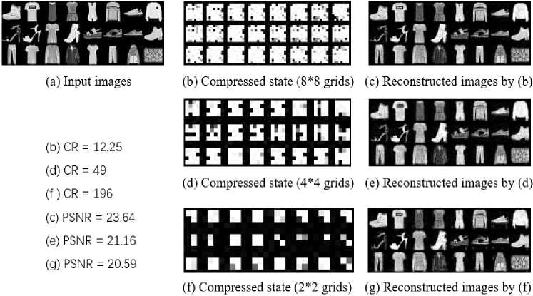
Figure 7: Quantum-Classical Autoencoder on Fashion-MNIST;

We compress input product states into intermediate representations in three different scales i.e. 8*8 grids, 4*4 grids and 2*2 grids. It should be that larger grids are benefit of saving more original input information, so that we could reconstruct better images from it and have a better PSNR score. We see it clearly in both Fig.6 and Fig.7. In contrast, the smaller intermediate representations will have higher CR. So we should achieve balance between them in the practical quantum information application.

III.3 Quantum feature engineering

Above two cases we present show the potential of developing the new concept of quantum feature engineering which is the quantum version of feature engineering in machine learning. It is generally recognized that deep learning model is a kind of effective models to implement feature engineering since it is capable of extracting feature information automatically from the raw data. Such as during the process of training a convolutional neural network, the convolutional kernels will be trained as feature detectors to recognize, extract and assemble valuable feature information which will be used in the subsequent machine learning task such as classification, regression or sequential analysis etc.. In analogy to this standpoint, HTN could be treated as a well-defined hybrid quantum classical model that is appropriate for quantum feature engineering. Although we have no formal definition of what quantum feature exactly is in the machine learning, we still start to investigate it involving quantum entanglement and fidelity by using TTN in our previous work(Liu et al., 2019). However, as a kind of typical regular tensor networks as we discussed before, TTN exposes some limitations on machine learning, and our analysis of the entanglement and fidelity show the deficiency on superficiality and coarse graining. Based on these, we believe that the HTN will be a good choice of quantum feature engineering method in the future work and help us to understand how quantum features such as entanglement and fidelity affect the performance of machine learning.

Discussion

We propose the hybrid tensor networks that combining tensor networks with classical neural networks in a uniform framework in order to overcome the limitations of regular tensor networks in machine learning. Based on the numerical experiments, we conclude with the following observations. (1) Regular tensor networks are not competent to be the basic building block of deep learning due to the limitations of representation power i.e. the absence of nonlinearity, and the restriction of scalability. (2) HTN overcomes the deficiency on representation power of regular tensor network by introducing the nonlinear function from neural network units, and offers good performance in scalability. (3) HTN could be trained by the standard combination of BP and SGD algorithms which offers us infinite possibilities to design HTN following the deep learning ways. (4) HTN serves as an applicable implementation of quantum feature engineering that could be simulated on classical computer.

There are some interesting and potential research subjects to be left in our future works. The first one is to do deep learning on quantum entanglement data by HTN. Our preliminary experiments in this paper focus on dealing with product quantum states without entanglement, but it is naturally to extend HTN to the scenario of quantum entanglement data formed by MPS or PEPS etc., which neural network is incapable of. Moreover, there are some works focus on tensor network based quantum circuit which shows us the interesting way to do quantum machine learning (Huggins et al., 2018). And also, some works focus on the quantum-classical machine learning by using parameter quantum circuit (Xia and Kais, 2019; Otterbach et al., 2017; Zhu et al., 2019; Sweke et al., 2019; Vinci et al., 2019). Inspired from these works, the HTN is able to be implemented by parameter quantum circuit in the future. In this case, the training algorithm should be revised to guarantee the isometry of each local tensor in the HTN.

Acknowledgments.— DL is grateful to Shi-ju Ran for helpful discussions. And this work was supported by the Science & Technology Development Fund of Tianjin Education Commission for Higher Education (2018KJ217), the China Scholarship Council (201609345008).

References

- Verstraete et al. (2008a) Frank Verstraete, Valentin Murg, and J. Ignacio Cirac, “Matrix product states, projected entangled pair states, and variational renormalization group methods for quantum spin systems,” Advances in Physics 57, 143–224 (2008a), arXiv:0907.2796 .
- Orús (2014a) Román Orús, “A practical introduction to tensor networks: Matrix product states and projected entangled pair states,” Annals of Physics 349, 117 (2014a), arXiv:1306.2164 .
- Orús (2014b) Román Orús, “Advances on tensor network theory: symmetries, fermions, entanglement, and holography,” The European Physical Journal B 87, 280 (2014b), arXiv:1407.6552 .
- Ran et al. (2017) Shi-Ju Ran, Emanuele Tirrito, Cheng Peng, Xi Chen, Gang Su, and Maciej Lewenstein, “Review of tensor network contraction approaches,” (2017), arXiv:1708.09213 .
- Orús (2019) Román Orús, “Tensor networks for complex quantum systems,” Nature Reviews Physics , 1–13 (2019).
- Efthymiou et al. (2019) Stavros Efthymiou, Jack Hidary, and Stefan Leichenauer, “Tensornetwork for machine learning,” arXiv preprint arXiv:1906.06329 (2019).
- Roberts et al. (2019) Chase Roberts, Ashley Milsted, Martin Ganahl, Adam Zalcman, Bruce Fontaine, Yijian Zou, Jack Hidary, Guifre Vidal, and Stefan Leichenauer, “Tensornetwork: A library for physics and machine learning,” arXiv preprint arXiv:1905.01330 (2019).
- Sun et al. (2020) Zheng-Zhi Sun, Shi-Ju Ran, and Gang Su, “Tangent-space gradient optimization of tensor network for machine learning,” arXiv preprint arXiv:2001.04029 (2020).
- Stoudenmire and Schwab (2016) E. Miles Stoudenmire and David J. Schwab, “Supervised learning with tensor networks,” Advances in Neural Information Processing Systems 29, 4799–4807 (2016), 1605.05775 .
- Han et al. (2017) Zhao-Yu Han, Jun Wang, Heng Fan, Lei Wang, and Pan Zhang, “Unsupervised generative modeling using matrix product states,” (2017), arXiv:1709.01662 .
- Liu et al. (2019) Ding Liu, Shi-Ju Ran, Peter Wittek, Cheng Peng, Raul Blázquez García, Gang Su, and Maciej Lewenstein, “Machine learning by unitary tensor network of hierarchical tree structure,” New Journal of Physics 21, 073059 (2019).
- Cichocki et al. (2016) Andrzej Cichocki, Namgil Lee, Ivan Oseledets, Anh-Huy Phan, Qibin Zhao, Danilo P. Mandic, and Others, “Tensor networks for dimensionality reduction and large-scale optimization: Part 1 low-rank tensor decompositions,” Foundations and Trends® in Machine Learning 9, 249–429 (2016).
- Cichocki et al. (2017) Andrzej Cichocki, Anh-Huy Phan, Qibin Zhao, Namgil Lee, Ivan Oseledets, Masashi Sugiyama, Danilo P. Mandic, and Others, “Tensor networks for dimensionality reduction and large-scale optimization: Part 2 applications and future perspectives,” Foundations and Trends® in Machine Learning 9, 431–673 (2017).
- Cheng et al. (2019) Song Cheng, Lei Wang, Tao Xiang, and Pan Zhang, “Tree tensor networks for generative modeling,” (2019).
- Li and Zhang (2018) Zhuan Li and Pan Zhang, “Shortcut matrix product states and its applications,” arXiv preprint arXiv:1812.05248 (2018).
- Kossaifi et al. (2017) Jean Kossaifi, Zachary Lipton, Aran Khanna, Tommaso Furlanello, and Anima Anandkumar, “Tensor regression networks,” arXiv (2017).
- Ran (2019a) Shi-Ju Ran, “Bayesian tensor network and optimization algorithm for probabilistic machine learning,” arXiv preprint arXiv:1912.12923 (2019a).
- Ran et al. (2019) Shi-Ju Ran, Zheng-Zhi Sun, Shao-Ming Fei, Gang Su, and Maciej Lewenstein, “Quantum compressed sensing with unsupervised tensor network machine learning,” arXiv preprint arXiv:1907.10290 (2019).
- Huggins et al. (2018) William Huggins, Piyush Patel, K. Birgitta Whaley, and E. Miles Stoudenmire, “Towards quantum machine learning with tensor networks,” Quantum Science and Technology (2018).
- Benedetti et al. (2018) Marcello Benedetti, Delfina Garcia-Pintos, Yunseong Nam, and Alejandro Perdomo-Ortiz, “A generative modeling approach for benchmarking and training shallow quantum circuits,” (2018).
- Bhatia et al. (2019) Amandeep Singh Bhatia, Mandeep Kaur Saggi, Ajay Kumar, and Sushma Jain, “Matrix product state–based quantum classifier,” Neural computation 31, 1499–1517 (2019).
- Ran (2019b) Shi-Ju Ran, “Efficient encoding of matrix product states into quantum circuits of one-and two-qubit gates,” arXiv preprint arXiv:1908.07958 (2019b).
- Wang et al. (2020) Kunkun Wang, Lei Xiao, Wei Yi, Shi-Ju Ran, and Peng Xue, “Quantum image classifier with single photons,” arXiv preprint arXiv:2003.08551 (2020).
- Leshno et al. (1993) Moshe Leshno, Vladimir Ya Lin, Allan Pinkus, and Shimon Schocken, “Multilayer feedforward networks with a nonpolynomial activation function can approximate any function,” Neural networks 6, 861–867 (1993).
- Hornik (1991) Kurt Hornik, “Approximation capabilities of multilayer feedforward networks,” Neural networks 4, 251–257 (1991).
- Glasser et al. (2018) Ivan Glasser, Nicola Pancotti, and J Ignacio Cirac, “Supervised learning with generalized tensor networks,” arXiv preprint arXiv:1806.05964 (2018).
- Verstraete et al. (2008b) Frank Verstraete, Valentin Murg, and J Ignacio Cirac, “Matrix product states, projected entangled pair states, and variational renormalization group methods for quantum spin systems,” Advances in Physics 57, 143–224 (2008b).
- Glasser et al. (2019) Ivan Glasser, Ryan Sweke, Nicola Pancotti, Jens Eisert, and Ignacio Cirac, “Expressive power of tensor-network factorizations for probabilistic modeling,” in Advances in Neural Information Processing Systems (2019) pp. 1496–1508.
- Chen et al. (2018) Jing Chen, Song Cheng, Haidong Xie, Lei Wang, and Tao Xiang, “Equivalence of restricted boltzmann machines and tensor network states,” Physical Review B 97, 085104 (2018).
- LeCun et al. (1995) Yann LeCun, Yoshua Bengio, et al., “Convolutional networks for images, speech, and time series,” The handbook of brain theory and neural networks 3361, 1995 (1995).
- Hochreiter and Schmidhuber (1997) Sepp Hochreiter and Jürgen Schmidhuber, “Long short-term memory,” Neural computation 9, 1735–1780 (1997).
- Goodfellow et al. (2014) Ian Goodfellow, Jean Pouget-Abadie, Mehdi Mirza, Bing Xu, David Warde-Farley, Sherjil Ozair, Aaron Courville, and Yoshua Bengio, “Generative adversarial nets,” in Advances in neural information processing systems (2014) pp. 2672–2680.
- Vaswani et al. (2017) Ashish Vaswani, Noam Shazeer, Niki Parmar, Jakob Uszkoreit, Llion Jones, Aidan N Gomez, Łukasz Kaiser, and Illia Polosukhin, “Attention is all you need,” in Advances in neural information processing systems (2017) pp. 5998–6008.
- Goodfellow et al. (2016) Ian Goodfellow, Yoshua Bengio, and Aaron Courville, Deep learning (MIT press, 2016).
- Abadi et al. (2016) Martín Abadi, Paul Barham, Jianmin Chen, Zhifeng Chen, Andy Davis, Jeffrey Dean, Matthieu Devin, Sanjay Ghemawat, Geoffrey Irving, Michael Isard, et al., “Tensorflow: A system for large-scale machine learning,” in 12th USENIX Symposium on Operating Systems Design and Implementation (OSDI 16) (2016) pp. 265–283.
- Paszke et al. (2017) Adam Paszke, Sam Gross, Soumith Chintala, Gregory Chanan, Edward Yang, Zachary DeVito, Zeming Lin, Alban Desmaison, Luca Antiga, and Adam Lerer, “Automatic differentiation in pytorch,” (2017).
- Kingma and Ba (2014) Diederik P Kingma and Jimmy Ba, “Adam: A method for stochastic optimization,” arXiv preprint arXiv:1412.6980 (2014).
-
Note (1)
The code of the implementation is available at
https://github.com/dingliu0305/Hybrid-Tensor-Network. -
Note (2)
The code of the implementation is available at
https://github.com/dingliu0305/Hybrid-Tensor-Network. - Xia and Kais (2019) Rongxin Xia and Sabre Kais, “Hybrid quantum-classical neural network for generating quantum states,” arXiv preprint arXiv:1912.06184 (2019).
- Otterbach et al. (2017) JS Otterbach, R Manenti, N Alidoust, A Bestwick, M Block, B Bloom, S Caldwell, N Didier, E Schuyler Fried, S Hong, et al., “Unsupervised machine learning on a hybrid quantum computer,” arXiv preprint arXiv:1712.05771 (2017).
- Zhu et al. (2019) Daiwei Zhu, Norbert M Linke, Marcello Benedetti, Kevin A Landsman, Nhung H Nguyen, C Huerta Alderete, Alejandro Perdomo-Ortiz, Nathan Korda, A Garfoot, Charles Brecque, et al., “Training of quantum circuits on a hybrid quantum computer,” Science advances 5, eaaw9918 (2019).
- Sweke et al. (2019) Ryan Sweke, Frederik Wilde, Johannes Meyer, Maria Schuld, Paul K Fährmann, Barthélémy Meynard-Piganeau, and Jens Eisert, “Stochastic gradient descent for hybrid quantum-classical optimization,” arXiv preprint arXiv:1910.01155 (2019).
- Vinci et al. (2019) Walter Vinci, Lorenzo Buffoni, Hossein Sadeghi, Amir Khoshaman, Evgeny Andriyash, and Mohammad H Amin, “A path towards quantum advantage in training deep generative models with quantum annealers,” arXiv preprint arXiv:1912.02119 (2019).