On Restricting Real-Valued Genotypes
in Evolutionary Algorithms

Abstract

Real-valued genotypes together with the variation operators, mutation and crossover, constitute some of the fundamental building blocks of Evolutionary Algorithm s. Real-valued genotypes are utilized in a broad range of contexts, from weights in Artificial Neural Network s to parameters in robot control systems. Shared between most uses of real-valued genomes is the need for limiting the range of individual parameters to allowable bounds. In this paper we will illustrate the challenge of limiting the parameters of real-valued genomes and analyse the most promising method to properly limit these values. We utilize both empirical as well as benchmark examples to demonstrate the utility of the proposed method and through a literature review show how the insight of this paper could impact other research within the field. The proposed method requires minimal intervention from Evolutionary Algorithm practitioners and behaves well under repeated application of variation operators, leading to better theoretical properties as well as significant differences in well-known benchmarks.

1 Introduction

Evolutionary Algorithms (EAs) are a class of optimization algorithms that take inspiration from nature [5]. By taking inspiration from biological concepts such as hereditary traits, genotype - phenotype distinction, mutation, and survival of the fittest, EAs have been used to solve many challenging problems [3]. Many different encodings can be used to implement a genotype [17], among them is the real-valued genotype —a vector in $\mathbb{R}^{n}$ [8]. One often overlooked aspect of real-valued genotypes is the necessity to restrict the values to task specific bounds [19]. Restricting the values is fundamental since very few problems have infinite domains and because restrictions makes the search space feasible to explore [18].

In this paper, we demonstrate the challenges of restricting real-valued genotypes and the effect these limitations have on the distribution of values in the genome. We start by introducing the theoretical problem and how restriction can affect the distribution. We then show that this problem is not simply a theoretical possibility; by optimizing benchmark functions we show that results diverge by solely varying the restriction function. We also look at the literature to gain an impression of how this problem could affect other EA practitioners.

The contribution of our paper is a better understanding of how value restriction affects real-valued genotypes in EAs. In addition we show that this is a topic deserving of more scrutiny by the wider EA community through a literature overview of both well known EA frameworks and a review of conference proceedings. By showing both the theoretical as well as the practical side of this challenge, we hope that other researchers become aware of the need for better restriction functions for real-valued genotypes and can utilize the results presented here in future research.

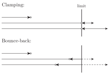
Figure 1: By clamping the values in a real-valued genome the values will tend towards the limits of the bounds. The proposed Bounce-back function reflects values that exceed the limits back inside the bounds, resulting in a uniform distribution inside the bounds.

2 Background

When designing a restriction function for real values, it is intuitive to create some form of a clamp method which ensures that a value does not exceed desired bounds. In the literature few articles have been dedicated to understanding the effect a restriction function could have on the evolutionary process. In [1] the authors compare different restriction methods on the result of evolving with Differential Evolution (DE) and showed that the results are impacted by the choice of restriction function. The paper [19] extended on this work by understanding which type of inheritance model functioned with different restriction functions and as a by-product illustrated how these different restriction functions can alter the search landscape. A larger review of different components that contribute to the evolutionary process in DE were undertaken in [18], in this review article the authors showed that the choice of restriction function can have a significant impact on the results, a result backed by a very comprehensive comparison on different benchmark functions. However, even with these articles, that show significant impact on results solely on the basis of the restriction function, it is our impression that few EA practitioners heed these warnings and make appropriate accommodations in regards to restricting real-valued genotypes.

To gain insight into the practises of restricting real-valued genotypes within the wider EA community, we conducted a limited literature review. We first began with identifying some of the larger open-source frameworks for implementing EAs to see how value restriction is implemented.

DEAP [6] is one of the more popular Python based frameworks for implementing EAs. Looking through the source code of this framework, two functions implement genome value restriction, ‘cxSimulatedBinaryBounded’ and ‘mutPolynomialBounded’. Both of these functions utilizes the Clamped function to limit real-valued genomes. SFERESv2 [13] is another well known framework implemented in C++. It too implements value restriction for real-valued genotypes as can be seen in the genotype definition in ‘evo_float.hpp’. The restriction function is implemented in ‘put_in_range’ and is equivalent to the Clamped function. Both of these frameworks cite the same source when it comes to their implementation of real-valued genomes and restriction, NSGA-II, a widely used Multi-Objective Evolutionary Algorithm [4]. Consulting the source-code of this algorithm, it can be seen that this too implements restriction through the Clamped function.

To evaluate whether or not the observations about evolutionary frameworks are representative for the community, we conducted a small review of the main proceedings from GECCO 2019 and the 2019 and 2020 EvoAPPS proceedings. To evaluate if the results of a paper could be susceptible to the challenges, identified in this paper, we first identified experiments utilizing real-valued genotypes, we then tried to identify if the authors discuss their strategy for value restriction or if anything could be discerned from the source of the experiments. The summary of our results can be seen in Table 1.

Table 1: Overview of real-valued genomes and limitation function in previous conference main proceedings.

	GECCO’19	EvoAPPS 2019	EvoAPPS 2020
Total number of papers	173	42	44
Uses real-valued genotype	37 ($21\%$)	11 ($26\%$)	10 ($22\%$)
Comments on value restriction	4	3	1

From the overview, we can see that real-valued genotypes are used in a large fraction of papers in these previous conferences. However, of those that could be identified to use some form of restriction only four papers in GECCO’19, three papers in EvoAPPS 2019 and one paper from EvoAPPS 2020 were found. Of the four papers in GECCO’19 two used strategies that can mitigate the challenges identified in this paper [7, 14], with one of those being our contribution, while the other two papers used the Clamped function. Of the three papers identified in EvoAPPS 2019 two would not be affected, one not using Gaussian mutation [10], another is our previous contribution using the methods proposed here [15], while the last one used the Clamped method. From EvoAPPS 2020, one paper was identified to not be susceptible [16] by only using uniform random mutation between allowable bounds instead of Gaussian mutation.

3 Methods

Several possible functions can be devised for limiting individual genes in real-valued genotypes [1]. The easiest and most straight forward limitation function is to clamp the value to the given bounds. The function is defined as follows

$$clamp(v,min,max)=\begin{cases}min\text{ if }v<min\\ max\text{ if }v>max\\ v\text{ otherwise}\end{cases}$$ (1)

where $v$ is the value to limit and $[min,max]$ are the bounds to apply for the value. This function will be used as the baseline to compare against the proposed Bounce-back method as it can be seen as the default when limiting real numbers and is the only one implemented in the EA frameworks reviewed. We will refer to this function as Clamped for the remainder of this text.

The proposed limit function, which we will call Bounce-back restriction (also known as reflection [1]), is defined as follows

$$\text{\it bounce-back}(v,min,max)=\begin{cases}min+(min-v)\text{ if }v<min\\ max-(v-max)\text{ if }v>max\\ v\text{ otherwise}\end{cases}$$ (2)

where, again, $v$ is the value to limit and $[min,max]$ are the bounds to apply for the value. The effect of the Bounce-back function is to redirect out-of-bounds values by the amount that the value is outside of the limits. The effect is illustrated in Figure 1. The function is independent of both mutation and crossover operators and can be applied in-between or after variation to ensure the genome is within given bounds. Compared to other restriction functions, such as wrapping, re-initialization and re-sampling[1], the Bounce-back function results in values in the current vicinity of the solution while also having minimum computational impact.

One thing to note about the Bounce-back function, as defined in Equation 2, is that it is not guaranteed to result in values within the given bounds. This can happen when the value $v>max+(max-min)$ or $v<min-(max-min)$. This can either be solved by continued application of the restriction function until the value is within bounds or limiting the difference in Equation 2 with the Clamped function. The later solution was utilized when limiting the distribution in Figure 2.

To demonstrate the unwanted properties of the clamp function and how these properties are not present in the Bounce-back function, we will first take an empirical approach to restricting real-valued genotypes with Gaussian perturbation.

4 Empirical analysis

To understand why using the clamp function with real-valued genomes can be problematic we will begin by looking at how the function affects the Gaussian distribution. In Figure 2 the result of applying the two limiting functions to the Gaussian distribution is shown. The grey area shows the original Gaussian distribution while the colored areas represent the respective limitation functions as applied. This example is akin to mutating a value that is on or near the bound with Gaussian perturbation before restricting the value to be less than the bound. As can be seen from the figure, the Bounce-back function result in a distribution that is equivalent with the Gaussian distribution. Applying the clamping function results in a distribution that is heavily biased towards the ‘limit’. This shows the problem with simply clamping a value to the desired bounds, the value will be skewed towards the bounds because all values above the limit is restricted to become exactly the limit, as illustrated in Figure 1.

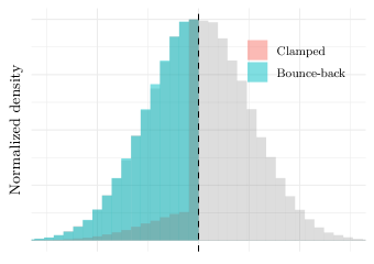
Figure 2: The resulting distributions of applying the limit functions to a Gaussian distribution, in grey, with mean equal to the ‘limit’ value marked with a dashed line. This is analogous to mutating a value at ‘limit’ with Gaussian mutation and then restricting the value to be less than the ‘limit’. The Bounce-back distribution follows the Gaussian distribution while the Clamped distribution is skewed towards the ‘limit’.

1:input $n$ $\triangleright$ Number of values in genome

2:input $cycles$ $\triangleright$ Number of times to simulate mutation

3:input $\sigma$ $\triangleright$ Standard deviation of Gaussian perturbation

4:$genome\leftarrow\mathcal{U}(0,1)^{n}$ $\triangleright$ Create a vector of $\mathbb{R}^{n}$, uniformly distributed

5:for $n\leftarrow 0$ to cycles do

6:     for $i\leftarrow 0$ to $n$ do

7:         $genome_{i}\leftarrow\mathcal{N}(genome_{i},\sigma)$ $\triangleright$ Apply Gaussian mutation

8:         if $genome_{i}<0.0$ or $genome_{i}>1.0$ then

9:              $genome_{i}\leftarrow restrict(genome_{i})$ $\triangleright$ Apply restriction, if outside bounds

10:         end if

11:     end for

12:end for

13:return $genome$

Algorithm 1 Simulating mutation and value restriction of real-valued genotypes. ‘restrict’ is either the Clamped or Bounce-back function.

To visualize how the two limitation functions will affect a real-valued genome we created Algorithm 1 which simulate how repeated application of Gaussian perturbation and restriction creates different distributions of values dependent on the limit functions. Figure 3 shows the distribution of values after running Algorithm 1 with $n$ equal to $50000$, $cycles$ set to $100$ and $\sigma=0.1$. In the figure it can be seen that the distribution of the Clamped function is heavily skewed towards the bounds while the Bounce-back function has a much more uniform distribution.

To ensure that the distribution of the Bounce-back limitation is uniformly distributed, we performed a One-sample Kolmogorov-Smirnov test [12] comparing the two distributions in Figure 3 with a uniform distribution. The results show that the Clamped distribution is statistically significant different from a uniform distribution, $p\ll 0.005$, while the Bounce-back distribution is not significantly different, $p>0.1$.

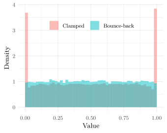
Figure 3: The resulting distributions of generating $50000$ uniform values between $[0,1]$, perturbing each value with a Gaussian, with $\sigma=0.1$, and then limiting the value to the range $[0,1]$. The perturbation-limitation cycle was run $100$ times.

To understand how the input parameters of Algorithm 1 impact the output, we varied the two parameters, $cycles$ and $\sigma$. We will postulate that the number of reals, $n$, will not impact the underlying distribution and the effect of changing this parameter is to give a better or worse impression of the underlying distribution. The results of changing the input parameters are shown in Figure 4 and Figure 5, for number of $cycles$ and varying the standard deviation respectively. Changing the number of $cycles$, shown in Figure 4, does not have an effect on the resulting distribution which is as expected. Since the probability of the Gaussian mutation going out- or staying inside the bounds is symmetrical, the number of times mutation is applied should not effect the resulting distribution. For the standard deviation, shown in Figure 5, the results are slightly different. Here we can see an effect of increasing $\sigma$, which can be explained as a larger part of the initial uniform distribution having a probability of going out of bounds. For the Clamped function this results in more values restricted at the bounds as the standard deviation of the mutation increases. On the other hand, we can see that the Bounce-back function is not affected by changes in mutation and continues to be uniformly distributed.

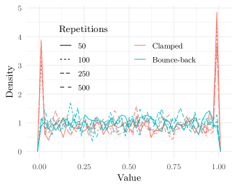
Figure 4: A comparison of how the number of repetitions of the perturbation-limitation cycle affects the resulting distribution. The distribution in the figure were generated from $1000$ uniform random values and perturbed by a Gaussian with $\sigma=0.1$.

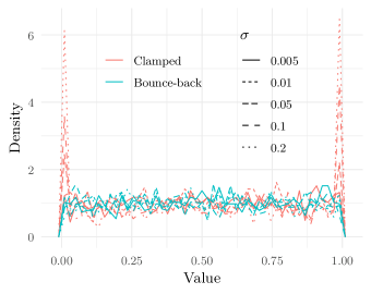
Figure 5: A comparison of how the standard deviation, $\sigma$, of the Gaussian affects the resulting distribution. The distribution in the figure were generated from $1000$ uniform random values and perturbed $100$ times.

5 Benchmark functions

To illustrate the potential impact of the limitation function, we applied the two limitation functions to a selection of benchmark problems [20]. All functions were optimized with a single objective $(\mu+\lambda)$ EA using tournament selection, Gaussian mutation, and no crossover operator. The benchmark problems are included to illustrate the challenge of limiting the genome to a specific range outside of theoretical considerations, as demonstrated in the previous section.

The following four functions are used as benchmark problems:

$$\frac{1}{4000}\sum_{i=1}^{N}x_{i}^{2}-\prod_{i=1}^{N}\cos\left(\frac{x_{i}}{\sqrt{i}}\right)+1$$ (3)

$$10N+\sum_{i=1}^{N}x_{i}^{2}-10\cos\left(2\pi x_{i}\right)$$ (4)

$$\sum_{i=1}^{N-1}\left(x_{i}^{2}+x_{i+1}^{2}\right)^{0.25}*\left[\sin^{2}(50*(x_{i}^{2}+x_{i+1}^{2})^{0.10}+1\right]$$ (5)

$$418.9828872724339*N-\sum_{i=1}^{N}x_{i}\sin\left(\sqrt{|x_{i}|}\right)$$ (6)

where $N$ is the size of the genome and $x_{i}$ is the value of gene $i$ in the genome. We will refer to equation (3) as Griewank, equation (4) as Rastrigin, equation (5) as Schaffer and equation (6) as Schwefel. The genotype was encoded as a vector of reals with a range of $[0,1]$, before being transformed into the range required by each benchmark task. Genotypes are randomly initiated based on a uniform distribution. To generate data, we first optimized the parameters for each function, selecting the best mutation rate $\sigma$, tournament size and probability of applying Gaussian mutation to gene $i$ - $P(M|i)$. The final parameters used to generate data are shown in Table 2.

Table 2: Algorithm parameters for each benchmark function. Parameters marked with ‘†’ were taken from [2].

	Griewank	Rastrigin	Schaffer	Schwefel
Generations†	2000
$(\mu+\lambda)$†	$100+100$
Size - $n$†	30
Repetitions	50
Tournament	10
$P(M|i)$	0.05
Mutation - ‘$\sigma$’	0.005	0.05	0.05	0.2
Range	$\pm 600$	$\pm 5.12$	$\pm 100$	$\pm 500$

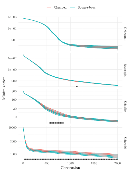
Figure 6: The mean and $95\%$ confidence interval for the population minimum aggregated over $50$ runs of each benchmark function. Differences are marked at the bottom of each graph in black, the difference is statistical significant using a Wilcoxon Rank Sum test over an interval of $10$ generations adjusted for the number of tests using Holm correction.

Figure 6 shows the mean and $95\%$ confidence interval of the population minimum for each benchmark function. Statistical significant differences between the two limitation functions are marked in black at the bottom of each plot and is the result of applying the Wilcoxon Rank Sum test on intervals of $10$ generations. To correct the p-value for the number of successive tests performed per row, Holm correction [9] was applied. The result show that only one benchmark function is sufficiently affected to lead to different results, however, both Rastrigin and Schaffer show diverging results at some points before converging. Based on the individual search parameters, shown in Table 2, we can also observe that larger $\sigma$ seems to induce larger differences.

6 Discussion

From the empirical analysis performed, it can be seen that the Clamped function skews the distribution of values towards the bounds of the range, as shown in Figure 2 and Figure 3. This property can be challenging when the genotype is based on real values that are translated into task applicable ranges during the phenotype conversion. The proposed Bounce-back function did not exhibit these properties resulting in no alteration of the underlying value distribution. When experimenting with different facets of mutation, Figure 4 and Figure 5, it was shown that the magnitude of the standard deviation had the most effect on the resulting value distribution. This can be understood as expanding the range of the Gaussian distribution applied at each value. As more values have the potential of being mutated near the bounds, more values will be restricted and end up at the extremities of the limit with the Clamped function. This leads to the observation that using a larger standard deviation in the mutation operator require more careful thought to which restriction function to apply.

The results in Figure 6 shows that the choice of restriction function can have an effect on benchmark problems, and is not just a theoretical problem. The effect of the restriction function followed closely the magnitude of the standard deviation used for mutation, detailed in Table 2, and illustrates the challenge that it can be difficult a priori to know the effect of the restriction function on any given task. One thing to point out about the benchmark tasks is that, except for Schwefel, the target value for all genes is $x_{i}=0$, which is in the middle of the range, away from the bounds. As the target value moves closer to the bounds, we would expect the effect of the restriction function to grow, which could also explain the larger difference observed with the Schwefel benchmark function. With real-world tasks where the optimal value is difficult or impossible to confirm, it is even more challenging to a priori predict the effect and interactions of the restriction function, making it paramount that the restriction function has minimal impact on the optimization process.

The literature review conducted showed that two popular EA frameworks utilizes the Clamped function for restriction, and that while many papers published at GECCO’19 and EvoAPPS 2019 and 2020 utilized real-valued genotypes, few papers discussed their use of restriction functions. A deeper dive into the source of NSGA-II, a foundational algorithm within the Multi-Objective Evolutionary Algorithm literature, also revealed the use of the Clamped function which could affect re-implementations. Although limited, the literature review does underscore how the findings in this paper could impact the broader research field. As shown previously, the restriction function is not guaranteed to lead to significantly different results, however, it is difficult to predict the effect beforehand.

The results shown in this paper has focused on restricting real-valued genotypes in EAs. One interesting direction to take this work in the future is to apply the same Bounce-back technique on particles in Particle Swarm Optimization (PSO) [11]. Because of the additional velocity attribute present in PSO the restriction function should take this into account when limiting so that the particles do not keep moving towards the bounds. In the same vein, it would be interesting to know if PSO is sensitive to the challenges presented in this paper, or if the collective behavior can mitigate the boundary effect shown in this paper.

7 Conclusion

In this paper we have shown that one of the most used functions for restricting real-valued genotypes behaves badly under repeated application of the variation operators. We therefore suggest a different function which result in a uniform distribution of values within the genome. The Bounce-back function is shown both empirically and in practise to lead to better distributions and requires minimal intervention from existing Evolutionary Algorithm implementations, while having a minimal computational impact. We also conducted a limited literature review which illustrated that other practitioners in the field of Evolutionary Algorithm s could be susceptible to the complications detailed in this paper. We hope that by illuminating this problem other researchers will become aware of the requirements for restricting real-valued genotypes, and can hopefully mitigate it with minimal effort in future work.

References

- [1] Arabas, J., Szczepankiewicz, A., Wroniak, T.: Experimental comparison of methods to handle boundary constraints in differential evolution. In: International Conference on Parallel Problem Solving from Nature. pp. 411–420. Springer (2010)
- [2] Brest, J., Greiner, S., Boskovic, B., Mernik, M., Zumer, V.: Self-adapting control parameters in differential evolution: A comparative study on numerical benchmark problems. IEEE transactions on evolutionary computation 10(6), 646–657 (2006)
- [3] Chiong, R., Weise, T., Michalewicz, Z.: Variants of Evolutionary Algorithms for Real-World Applications. Springer, Berlin Heidelberg (2012)
- [4] Deb, K., Agrawal, S., Pratap, A., Meyarivan, T.: A fast elitist non-dominated sorting genetic algorithm for multi-objective optimization: Nsga-ii. In: International conference on parallel problem solving from nature. pp. 849–858. Springer, Berlin, Heidelberg (2000)
- [5] Floreano, D., Mattiussi, C.: Bio-Inspired Artificial Intelligence: Theories, Methods, and Technologies. Intelligent Robotics and Autonomous Agents, MIT Press, Cambridge, MA (2008), http://infoscience.epfl.ch/record/118584
- [6] Fortin, F.A., De Rainville, F.M., Gardner, M.A., Parizeau, M., Gagné, C.: DEAP: Evolutionary algorithms made easy. Journal of Machine Learning Research 13, 2171–2175 (jul 2012)
- [7] Glasmachers, T.: Challenges of convex quadratic bi-objective benchmark problems. In: Proceedings of the Genetic and Evolutionary Computation Conference. p. 559–567. GECCO ’19, Association for Computing Machinery, New York, NY, USA (2019)
- [8] Herrera, F., Lozano, M., Verdegay, J.L.: Tackling real-coded genetic algorithms: Operators and tools for behavioural analysis. Artificial intelligence review 12(4), 265–319 (1998)
- [9] Holm, S.: A simple sequentially rejective multiple test procedure. Scandinavian journal of statistics 6(2), 65–70 (1979)
- [10] Iacca, G., Caraffini, F.: Compact optimization algorithms with re-sampled inheritance. In: Kaufmann, P., Castillo, P.A. (eds.) Applications of Evolutionary Computation. pp. 523–534. Springer International Publishing, Cham (2019)
- [11] Kennedy, J., Eberhart, R.: Particle swarm optimization. In: Proceedings of ICNN’95-International Conference on Neural Networks. vol. 4, pp. 1942–1948. IEEE, Perth, WA, Australia (1995)
- [12] Massey Jr, F.J.: The kolmogorov-smirnov test for goodness of fit. Journal of the American statistical Association 46(253), 68–78 (1951)
- [13] Mouret, J.B., Doncieux, S.: SFERESv2: Evolvin’ in the multi-core world. In: Proc. of Congress on Evolutionary Computation (CEC). pp. 4079–4086. IEEE, Barcelona, Spain (2010)
- [14] Nordmoen, J., Nygaard, T.F., Ellefsen, K.O., Glette, K.: Evolved embodied phase coordination enables robust quadruped robot locomotion. In: Proceedings of the Genetic and Evolutionary Computation Conference. p. 133–141. GECCO ’19, Association for Computing Machinery, New York, NY, USA (2019)
- [15] Nygaard, T.F., Martin, C.P., Torresen, J., Glette, K.: Evolving robots on easy mode: Towards a variable complexity controller for quadrupeds. In: Kaufmann, P., Castillo, P.A. (eds.) Applications of Evolutionary Computation. pp. 616–632. Springer International Publishing, Cham (2019)
- [16] Pontes-Filho, S., Lind, P., Yazidi, A., Zhang, J., Hammer, H., Mello, G.B.M., Sandvig, I., Tufte, G., Nichele, S.: Evodynamic: A framework for the evolution of generally represented dynamical systems and its application to criticality. In: Castillo, P.A., Jiménez Laredo, J.L., Fernández de Vega, F. (eds.) Applications of Evolutionary Computation. pp. 133–148. Springer International Publishing, Cham (2020)
- [17] Rothlauf, F.: Representations for Genetic and Evolutionary Algorithms, pp. 9–32. Springer Berlin Heidelberg, Berlin, Heidelberg (2006)
- [18] Tanabe, R., Ishibuchi, H.: Review and analysis of three components of the differential evolution mutation operator in MOEA/D-DE. Soft Computing 23(23), 12843–12857 (2019)
- [19] Wessing, S.: Repair methods for box constraints revisited. In: Esparcia-Alcázar, A.I. (ed.) Applications of Evolutionary Computation. pp. 469–478. Springer Berlin Heidelberg, Berlin, Heidelberg (2013)
- [20] Yao, X., Liu, Y., Lin, G.: Evolutionary programming made faster. IEEE Transactions on Evolutionary computation 3(2), 82–102 (1999)